Abstract
Dust weather is common and disastrous at the Tibetan Plateau. This study selected a typical case of dust weather and analyzed its main development mechanism in the northeast of the Tibetan Plateau, then applied six machine learning methods and a time series regression model to predict PM10 concentration in this area. The results showed that: (1) The 24-h pressure change was positive when the front intruded on the surface; convergence of vector winds with a sudden drop in temperature and humidity led by a trough on 700 hPa; a “two troughs and one ridge” weather situation appeared on 500 hPa while the cold advection behind the trough was strong and a cyclone vorticity was formed in the east of Inner Mongolia. (2) The trajectory of air mass from the Hexi Corridor was the main air mass path influencing Xining City, in this case, since a significant lag in the peak of PM10 concentration appeared in Xining City when compared with Zhangye City. (3) The Multiple Linear Regression was not only timely and effective in predicting the PM10 concentration but had great abilities for anticipating the transition period of particle concentration and the appearance date of maximum values in such dust weather. (4) The MA and MP in the clean period were much lower than that in the dust period; the PM10 of Zhangye City as an eigenvalue played an important role in predicting the PM10 of Xining City even in clean periods. Different from dust periods, the prediction effect of Random Forest Optimized by Bayesian hyperparameter was superior to Multiple Linear Regression in clean periods.
1. Introduction
Dust weather is common and disastrous at the Tibetan Plateau. It not only seriously reduces the quality of the ecological environment but causes great damage to the social economy and human health [1,2,3,4]. Dust storm behavior varies based on five attributes that are wind speed, pressure, temperature, humidity, and surface type [5,6]. The dust events significantly increase the air pollutants PM2.5, CO, and O3, which are directly associated with the increase in the spread and severity of the pandemic [7]. Sandstorms are the primary source of air pollutants, dust, gases, fine particulate matter, and their long-distance transport [8,9]. The dust storms mainly occur in winter and early spring with high frequency, and the path moves gradually from south to north, which is closely coupled with the northward moving of the westerly jet from winter to spring over the Tibetan Plateau [10]. Past studies have shown that the Gobi Desert, Hexi Corridor, Qaidam Basin, Turpan Basin, and the edges of the Tarim and Junggar basins are identified as the main dust sources for the northern Tibetan Plateau [11,12]. The occurrences and developments of dust weather are closely related to cold air and geographical conditions; under the block of mountains, the PM10 concentrations increase significantly [13,14]. The aerosol optical depth (AOD) data and relevant meteorological parameters can be used to analyze the sandstorm and evaluate the temporal–spatial distributions with the evolution process of dust [15,16,17,18,19].
The applications of artificial Intelligence technology in the field of meteorology are mainly about various machine learning methods, including weather forecast, meteorological services, medical meteorology, and agricultural meteorological products [20,21,22]. Machine learning includes computational methods for learning from complex data. In the classification and evaluation of predicting meteorological elements or air pollution, some machine learning methods show the superiority and stability of fitting in nonlinear fields [23]. The case-based reasoning (CBR) approach with other AI techniques can be effective in predicting dust storm events as well as help in establishing effective counter policies [24]. By capturing temporal dependencies in the time series data, the Long Short-Term Memory (LSTM) achieved the better results in forecasting PM2.5 concentrations with low Root Mean Square Error, proving that this method can be effective for forecasting and controlling air pollution [25,26,27,28,29]. An online forecasting method based on Random Forest is proposed to predict the concentrations of three kinds of air pollutants (PM2.5, NO2, SO2), 24 h in advance, which achieves state-of-art performance [30]. A novel hybrid approach based on two-stage decomposition embeds sample entropy and extreme learning machine to forecast the concentration of particulate matter (PM10 and PM2.5), which overcomes the difficulties caused by the randomness and non-stationarity of air pollutant data [31,32]. The dust assimilation forecasting model is used to quantify the impact of assimilation on forecasts of a severe Asian dust storm [33]. Due to the lack of monitoring data limited by equipment, the Autoregressive Integrated Moving Average Model (ARIMA) and Multiple Linear Regression Additive Model based on linear interpolation are better [34,35]. Analyzing the data using different machine learning models, including linear regression, Artificial Neural Networks, and Long Short-Term Memory recurrent neural networks, considering the accuracy and capability of each method, and using different models to predict unhealthy pollution levels, are very important [36,37]. Various machine learning and deep learning methods estimating the concentration of particulate matter need more validation on a global scale.
The purpose of this study is to find the most suitable machine learning method for predicting PM10 in the northeast of the Tibetan Plateau. The structures are as follows: firstly, analyze the main development mechanisms by selecting a typical case of dust weather in the northeast of the Tibetan Plateau; secondly, apply the machine learning methods to the prediction of PM10 concentration and compare the advantages or disadvantages of the two most important methods in this area; finally, compare the prediction effects of the two machine learning methods during the cleaning period and dust period. In order to better capture the time, area, and intensity of the strong sandstorms at the Tibetan plateau, scientific and reasonable prediction and analysis were used in the study to reduce the adverse impact of sandstorms on the living environment and social economy.
2. Materials and Methods
2.1. Data Sources and Integration
The meteorological data provided by the Qinghai Provincial Meteorological Bureau included three-hourly surface observations and upper data from December 2020 to March 2021, mainly including: 500 pressure level (500 hPa) geopotential height, 500 hPa temperature, 500 hPa relative humidity, 500 hPa wind speed and direction, 700 pressure level (700 hPa) geopotential height, 700 hPa temperature, 700 hPa relative humidity, 700 hPa wind speed and direction, surface temperature, surface 24-h pressure change, surface relative humidity, surface minimum visibility.
The PM10 concentrations were from the national urban air quality real-time publishing platform of the China National Environmental Monitoring Centre, including the hourly and daily mean of PM10 concentration in Xining and Zhangye cities from December 2020 to March 2021 and from January 2022 to April 2022.
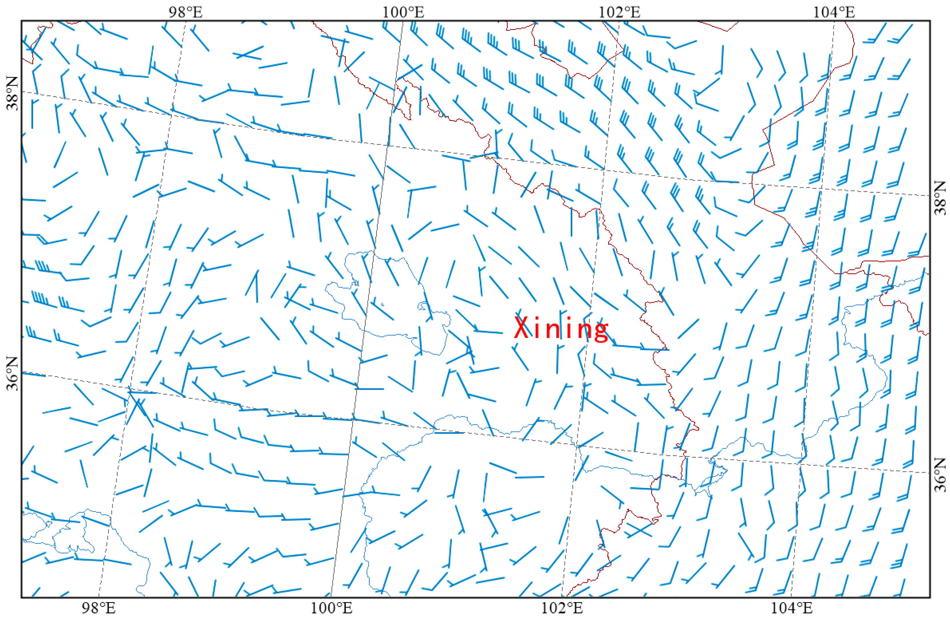
We adopted prediction products from the European Centre for Medium-Range Weather Forecasts (ECMWF) fine grid model from December 2020 to March 2021 and from January 2022 to April 2022 every three hours, which were provided by the Qinghai Provincial Meteorological Bureau, mainly including 700 hPa vector winds (Figure 1), 700 hPa temperature, 700 hPa relative humidity (the spatial resolution was 0.25° × 0.25°), and surface 24-h pressure change (the spatial resolution was 0.125° × 0.125°).
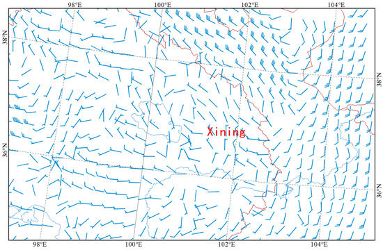
Figure 1.
One of the 700 hPa wind fields of ECMWF fine grid prediction products (the spatial resolution was 0.25° × 0.25°).
2.2. Model Introduction
2.2.1. Introduction to Machine Learning Methods
The Scikit-learn machine learning library was used, of which most of the functions could be divided into estimator and converter, and the estimator was a model used for the regression and prediction [38,39]. The samples were trained repeatedly by basic regression methods such as the Support Vector Machine (SVM), Multiple Linear Regression (MLR), K-Nearest Neighbor (KNN) in scikit-learn, and integrated methods, including the AdaBoost algorithm (Ada), Gradient Boosting Regression Tree (GBRT), and Random Forest (RF).
The Multiple Linear Regression (MLR) is one of the basic algorithms in machine learning methods. It adds more characteristic variables on the basis of univariate linear regression [40,41,42,43]. The regression model is as follows:
In the equation, represents the dependent variable with as the parameter, are the regression parameters to be solved, and are the characteristic variables.
The Random Forest (RF) algorithm compiles the information from multiple random trees (a group of decision trees) at the same time, and naturally incorporates the selection and interaction of eigenvalues in the learning process [44] so as to provide decision-making and selection for estimating pollutant concentration. The simulation variable values can be output by summarizing and averaging the individual simulations of all such composite trees. There are many hyperparameter optimization methods for Random Forests, including particle swarm optimization, genetic algorithm, differential evolution, Bayesian optimization, and so on. We selected Bayesian optimization in this study.
The Support Vector Machine (SVM) is a new statistical learning technique based on machine learning and generalization theories which use a hinge loss function to estimate the empirical risk and add a regularization term into the calculation process that can be solved non-linearly by the kernel method; it can be considered as a method to minimize the risk. Moreover, a generalization capability makes possible their application to modeling dynamical and non-linear data sets [45].
K-Nearest Neighbor (KNN) processes and classifies the data according to the distance between each site sample in the training and the verification sets and arranges all the distance values in order [46,47].
The AdaBoost integration algorithm reduces or increases the weight information by training samples each time, and then transfers the weight data to the next layer classifier for complex sample training [48].
The Gradient Boosting Regression Tree (GBRT) calculates the gradient direction of the residual reduction of each sample site by establishing multiple decision trees, obtains a decision tree composed of multiple leaf nodes, and obtains the gain of each leaf node for prediction [49].
The time series regression model used in this study was the Autoregressive Integrated Moving Average Model (ARIMA). The model transforms non-stationary time series into stationary time series, which is established by regressing the dependent variable to its lag value or the present and lag value of random error. This method was compared with the above six machine learning methods.
2.2.2. HYSPLIT Model
The HYSPLIT model (hybrid single particle Lagrangian integrated trajectory model) was developed jointly by the NOAA and Australian Meteorological Administration. It is used to calculate the simple air mass trajectory and simulate complex diffusion and deposition. The model can deal with a variety of physical processes and the transportation, diffusion, and settlement of pollutant emission sources with a variety of meteorological elements input fields [50].
Based on the HYSPLIT model, we set the parameters of the model and selected the GDAS (global data estimation system) meteorological data in March 2021 to analyze the air mass trajectory of dust weather in Xining City.
2.3. Evaluation and Analysis Approach
2.3.1. Air Quality Standards
This study evaluated and analyzed the air quality index (AQI) and PM10 concentration strictly according to the “Ambient Air Quality Standards” implemented in China from 1 January 2016 [51]. The evaluation standards are shown in Table 1:

Table 1.
PM10 concentration evaluation standards.
2.3.2. Dust Weather Grade Standard
The dust weather grades are shown in the Table 2.
Table 2.
Dust weather grade standard [52].
2.3.3. Valuation Method
In this study, the index to test the observed values and the predicted values were the Index of Agreement (IA), Mean Absolute Error (MA), and Mean Absolute Percentage Error (MP). The calculation formulas were as follows:
is the observed value, the predicted value, and is the mean observed value. The closer is to 1, the more accurate the predicted values are. The lower the of MA and MP, the less error the predicted values.
3. Analysis of Dust Weather from
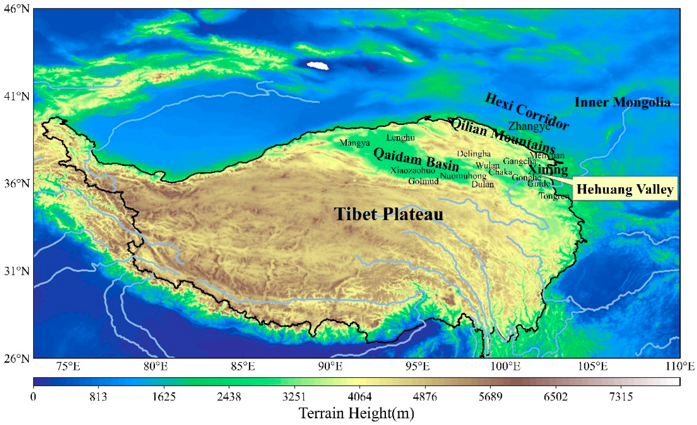
From the 14th to 20th March 2021, dust weather from north to south and west to east occurred in the northern area of China, with a wide range of influence and long duration, which was rated as the strongest dust in the past decade. This dust weather not only seriously interfered with the daily life and transportation of the public, causing casualties and disappearances in some areas, but also had a terrible impact on agriculture and animal husbandry. Figure 2 shows the terrain height of the Tibetan Plateau with the geographical locations of the Qaidam Basin, Qilian Mountains, Hexi Corridor, Inner Mongolia, and the main meteorological observation sites affected by this dust weather.

Figure 2.
Terrain height of the Tibetan Plateau, geographical location of Qaidam Basin, Qilian Mountains, Hexi Corridor, Inner Mongolia, and the main meteorological observation sites.
3.1. Dust Weather in the Northeast of Tibet Plateau
3.1.1. Dust Distribution
As shown in Figure 3, Inner Mongolia, the northern part of the North China Plain and the Hexi Corridor had the highest near-surface dust concentration and the largest accumulation of dry deposition. Nearly 20 meteorological observation sites of the northern Tibetan Plateau experienced dustfall, blowing sand, or short-term sandstorms.
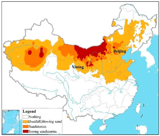
Figure 3.
Distribution of dust weather in northern China from 08:00 on 14 March to 11:00 on 16 March 2021 (Provided by the Central Meteorological Observatory of China.).
In the urban agglomeration of the Hehuang Valley in the northeast of the Tibetan Plateau, dust began appearing at 05:00 on the 16th and ended at 20:00 on the 20th, including dustfall and blowing sand in Xining, Menyuan, Guide, and Tongren cities. The visibility in Xining City was the worst from 23:00 on the 18th to 05:00 on the 19th, which was only 2 km. Dustfall and blowing sand appeared in Gangcha, Chaka, and Gonghe cities. In addition, sandstorms occurred in the Xiaozaohuo, Golmud, Nuomuhong, Dulan, and Wulan cities with visibility of less than 1 km, and the visibility of Xiaozaohuo at 23:00 on the 18th was as poor as 200 m.
The above showed that this dust weather lasted for a long time, which had strong intensity and a wide range of influence in the northeast of the Tibetan Plateau.
3.1.2. Surface Meteorological Conditions
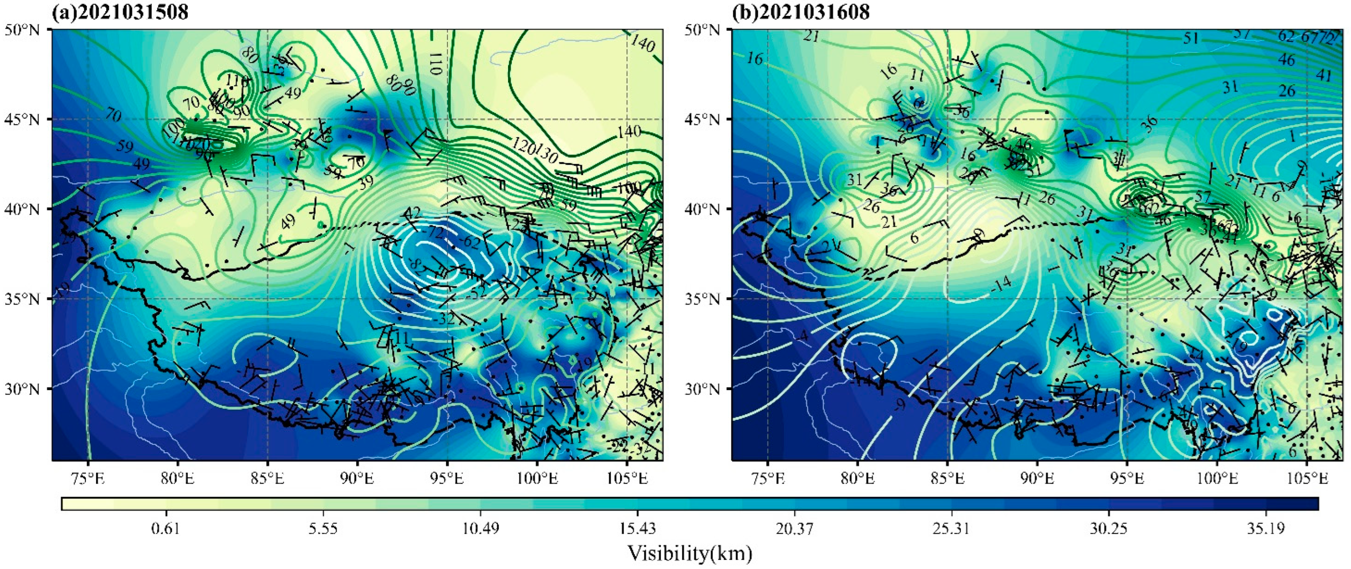
Figure 4 shows the distribution of the surface visibility, 24-h pressure change isolines, and the surface wind field at 08:00 on 15th and 16th of March. On the 15th, the 24-h pressure changes were significantly positive in the Hexi Corridor of the Tibetan plateau on the north side and Inner Mongolia with 14 hPa; a wide range of dust weather had occurred, which reduced the visibility to less than 1km in this area. The 24-h pressure change gradient was very significant, showing that there was a cold front passing through the area, and the surface wind speeds were strong. Until 08:00 on the 16th, 24-h pressure change was positive and exceeded 3 hPa in the Hehuang Valley, showing the cold front had completely invaded and carried large amounts of dust, resulting in a rapid decrease in the visibility and increase in the AQI in the area. The southern and southwestern regions of the Tibetan Plateau were not affected by the dust weather due to the high altitude and steep terrain.
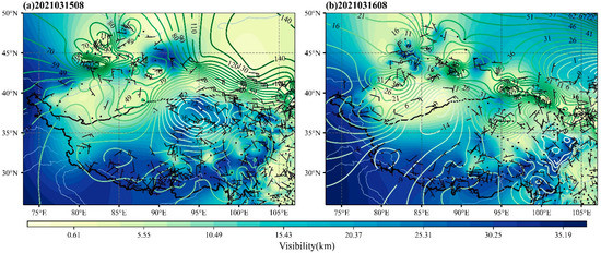
Figure 4.
Superposition diagram of 24-h pressure change (isolines), wind field, and minimum visibility on surface. (a) 08:00, 15 March 2021; (b) 08:00, 16 March 2021.
3.1.3. 700 hPa and 500 hPa Meteorological Conditions
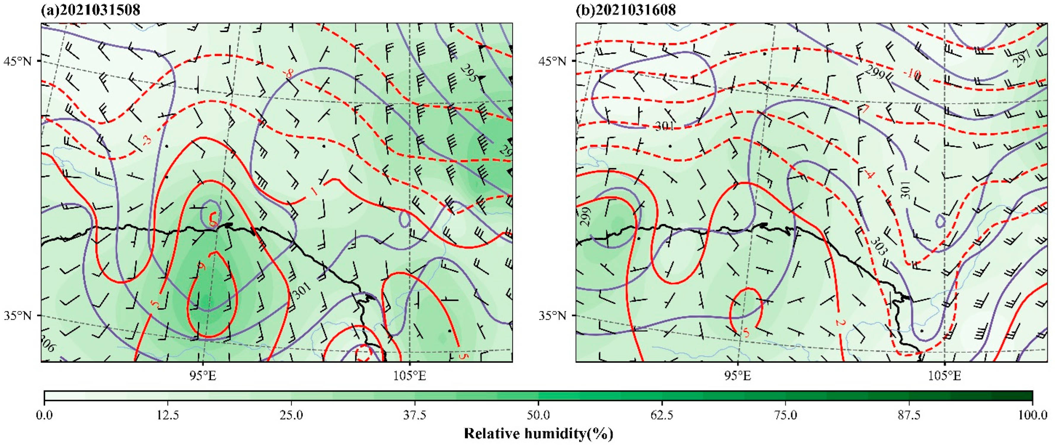
Figure 5 shows the 700 hPa meteorological conditions with geopotential height, temperature, wind field, and relative humidity. At 08:00 on March 16th, the contours and isotherms were denser than the previous day, and the isotherms moved southward causing significant cooling in most areas, especially affecting the Hehuang Valley where the temperatures at 700 hPa dropped to below 0 °C. It could be clearly observed that there was a trough deepening into the area that led to the convergence of vector winds. The distribution of relative humidity at 700 hPa was significantly lower than that of the previous day, especially at the northeastern Tibetan Plateau and the central Hexi Corridor where the relative humidity and temperatures decreased when the dust passed.
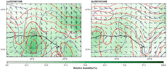
Figure 5.
Superposition diagram of geopotential height (purple contours), temperature (red isotherms), wind field, and relative humidity at 700 hPa. (a) 08:00, 15 March 2021; (b) 08:00, 16 March 2021.
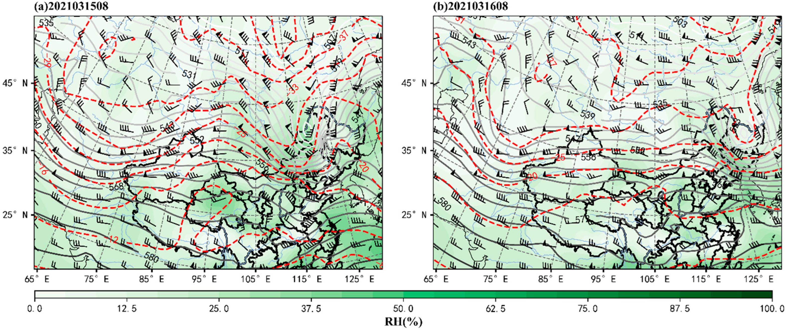
Figure 6 shows the 500 hPa meteorological conditions with geopotential height, temperature, wind field, and relative humidity. At 08:00 on March 15th, the atmospheric circulation of “two troughs and one ridge” with a large meridional scale and a maximum wind speed exceeding 32 m/s occurred. The cold advection behind the trough was strong and a cyclone vorticity was formed in the east of Inner Mongolia.
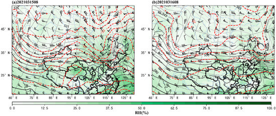
Figure 6.
Superposition diagram of geopotential height (black contours), temperature (red isotherms), wind field, and relative humidity at 500 hPa. (a) 08:00, 15 March 2021; (b) 08:00, 16 March 2021.
Such powerful dynamic transmission and cold advection at 700 hPa and 500 hPa would contribute to the formation and intensification of a cold front on the surface. The temperature difference between the upper strong cold advection and the surface was the main reason for the formation of the dry convective sandstorm.
3.2. HYSPLIT Backward Trajectory Model Analysis in Xining City
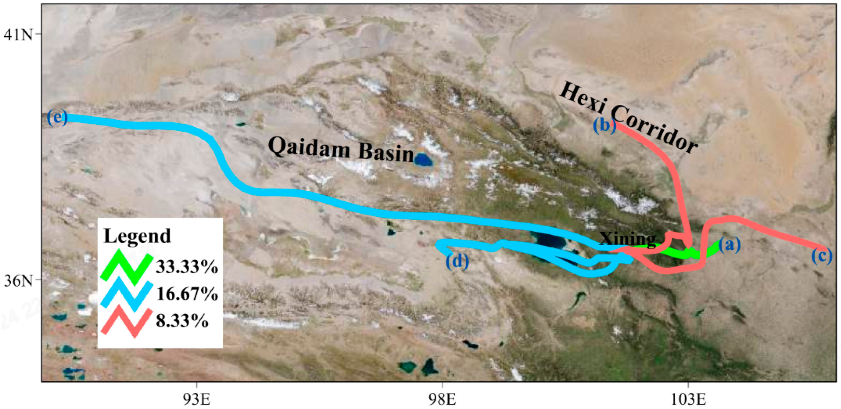
Trajectories were calculated using the NOAA-HYSPLIT model based on the meteorological field of March 2021. Xining City was selected as the starting point of the simulation to trace the air mass trajectory 48 h ahead at 08:00 every day. The simulation results showed that the main sources of air masses in Xining City included the westward path, the eastward path, the local source, and the northeast path of the backflow of the Hexi Corridor; 33.33% of them came from the local source and the easterly path, 16.67% came from the westward path, and 8.33% came from the Hexi Corridor (Figure 7).

Figure 7.
Cluster analysis of HYSPLIT backward trajectory in Xining City during March 2021.
The length of the air mass trajectory line of the westward path was the longest, which indicated that the wind force in this direction was strong, resulting in the air mass moving fast, and the air mass moved from high-altitude mountainous areas to low-altitude urban areas in this direction, therefore, the pressure differences were large and there were few pollutants making the transmission and diffusion conditions more favorable. The shortest trace of local source or eastward path indicated that, under the influence of calm or mild easterly wind, the air mass moved slowly from the east or stayed in place. At the same time, considering the terrain of the Hehuang Valley, the difference of pressure was slight with stable atmospheric stabilization, which resulted in poor transmission and diffusion conditions. The trajectory of air mass of the Hexi Corridor was shorter than that of the west, which indicated that it was blocked by the eastern edge of the Qilian Mountains in the northeast, resulting in slower movement, and converging with the east air flow, moving slowly into Xining City or staying in place. Lines a and b represent the main air mass paths in Xining City affected by this dust weather, and poor atmospheric diffusion conditions led to large amounts of dust carried by the air mass which accumulated in place.
3.3. Analysis of Meteorological Elements in Xining City
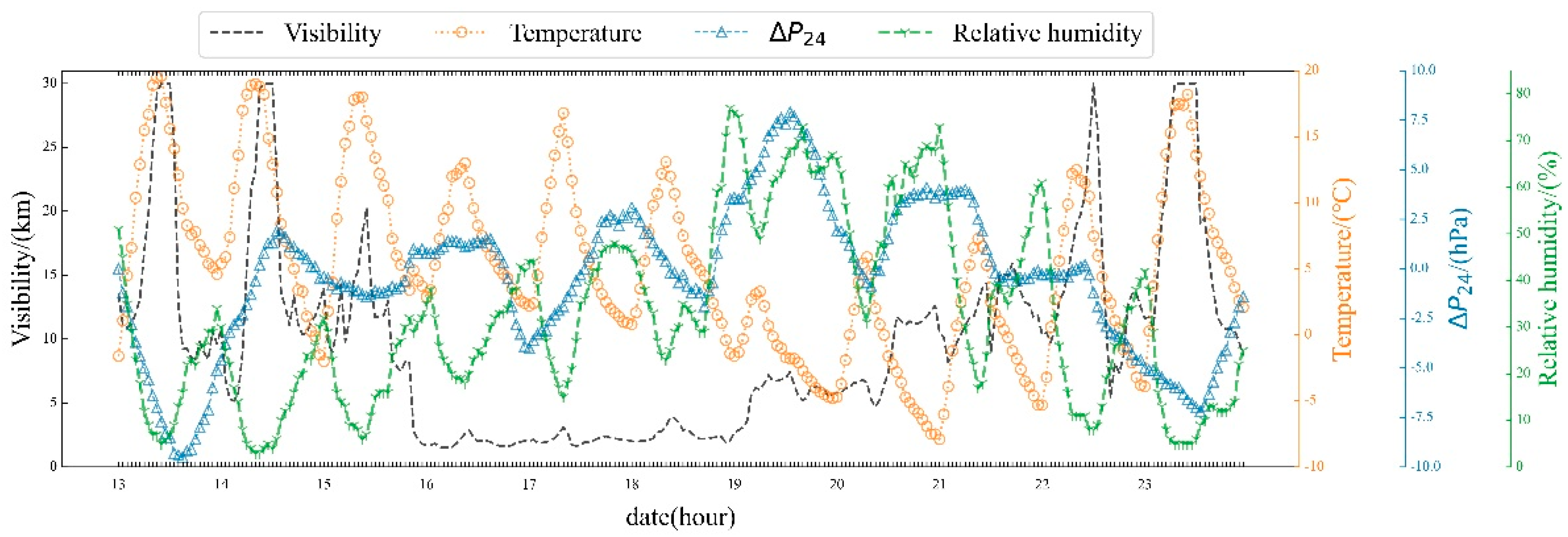
Xining City, the provincial capital city in the northeast of the Tibetan Plateau, was directly affected by this dust weather. The 24-h pressure change gradually increased at 11:00, which changed from negative (−0.6 hPa) to positive (0.3 hPa). At 21:00, visibility decreased rapidly to 2 km, indicating that the cold air had reached Xining City and carried large amounts of dust. Since on the 16th, the 24-h pressure changes in Xining City were mainly positive, the surface temperature decreased, and the southeast wind speeds increased day-by-day (as shown in Figure 8). Until on the 20th, the temperatures began to rise day-by-day, the 24-h pressure changes decreased, and the visibility improved, indicating that the dust weather affecting Xining City was coming to an end.
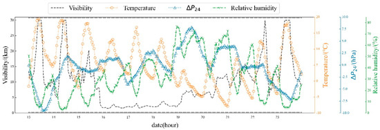
Figure 8.
Hourly variation curves of surface temperature, relative humidity, 24-h pressure change, and minimum visibility in Xining City from 13 to 23 March 2021.
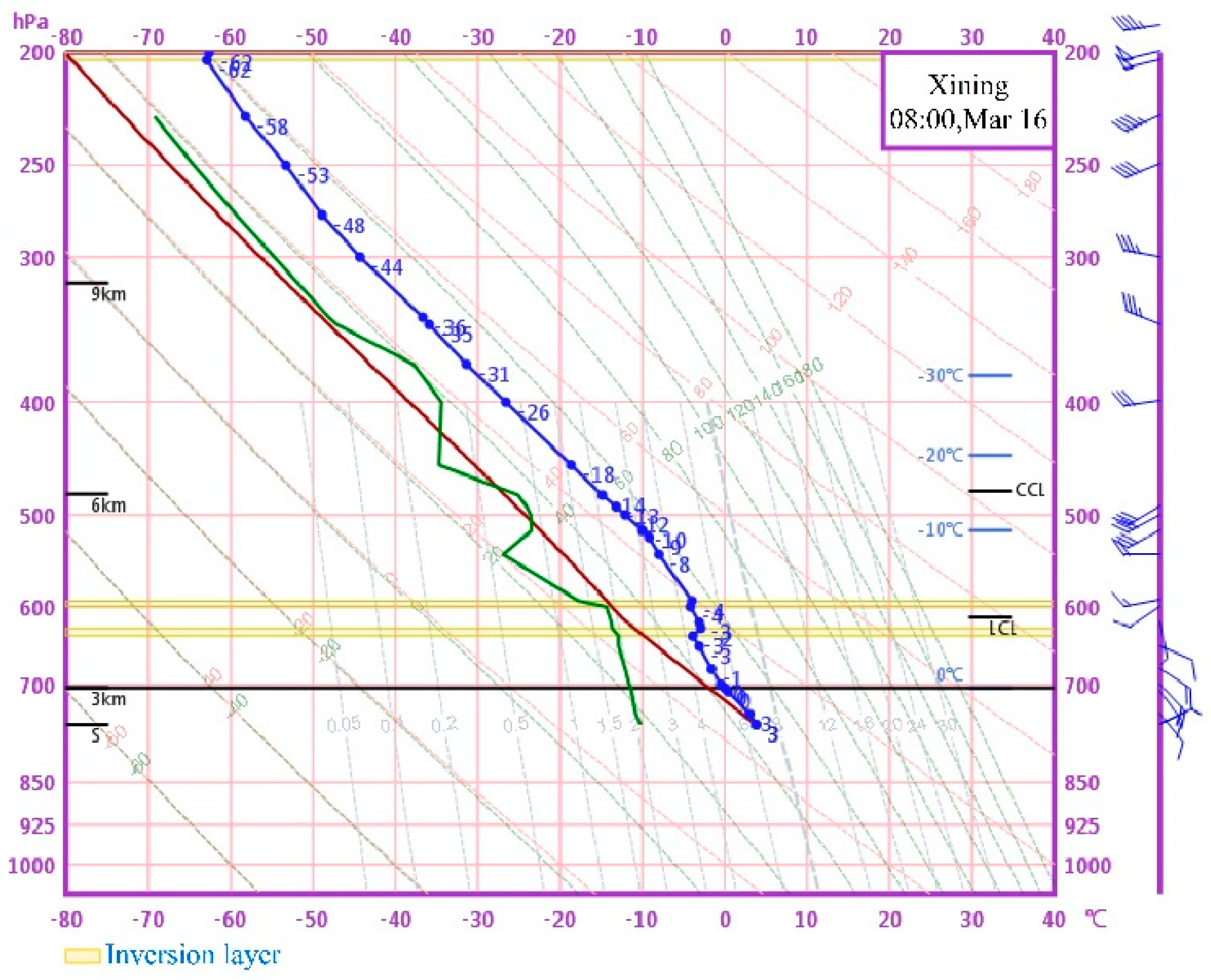
According to the structure of the T-lnp diagram (emagram) of Xining City at 08:00 on the 16th in Figure 9, the water vapor content of the whole layer over the area was poor, and two obvious inversion layers appeared between 700 hPa and 600 hPa, leading to the stable atmospheric stratification, which indicated that there were adverse meteorological conditions on the upper levels that were not conducive to the diffusion of pollutants.

Figure 9.
Structure of the T-lnp diagram (emagram) of Xining City at 08:00 on 16 March 2021.
3.4. Comparison of PM10 Concentrations between Xining and Zhangye Cities
Zhangye City was in the central Hexi corridor. The changes of surface PM10 concentration during this dust weather in Xining and Zhangye cities are shown in Figure 10. If Xining City was affected by the dust transport of path b, Zhangye City belonged to the upstream area of Xining City.
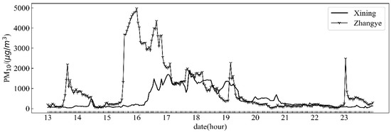
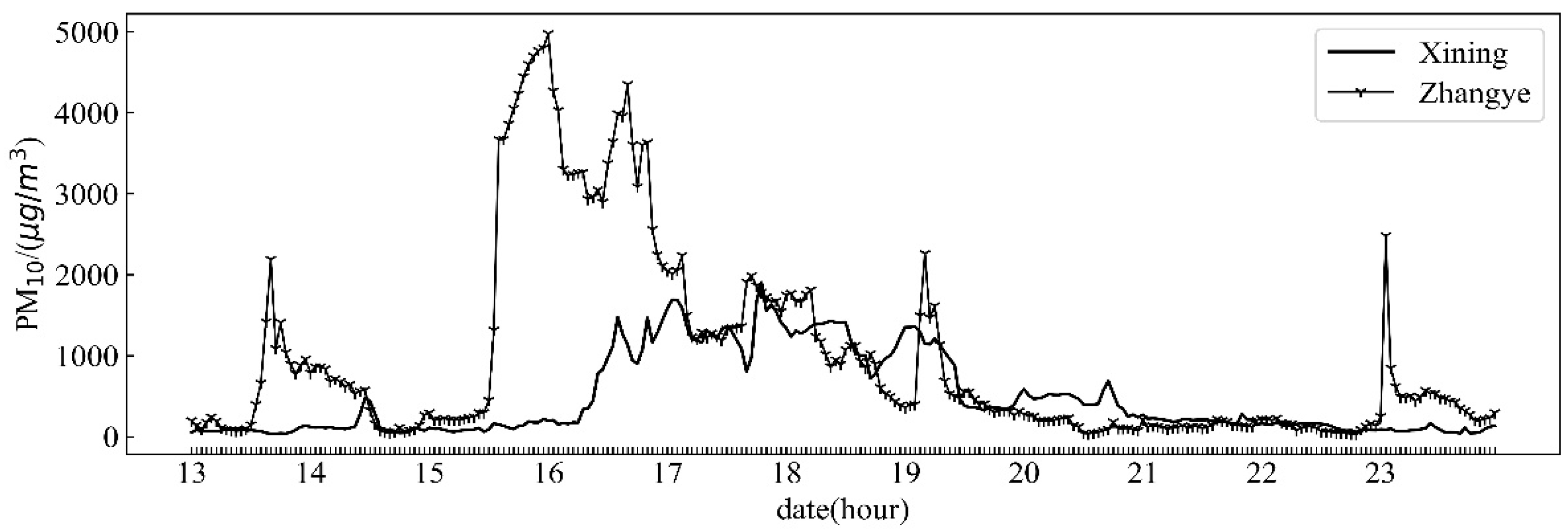
Figure 10.
Hourly variation curves of surface PM10 concentration in Xining and Zhangye cities from 13 to 23 March 2021.
The PM10 concentration in Zhangye City reached the peak of 2190 μg/m3 at 16:00 on the 13th, while the PM10 concentration reached the peak of 475 μg/m3 in Xining City at 11:00 on the 14th; the time differences between the two peaks were 19 h. At 13:00 on the 15th, the dust appeared again in Zhangye City, which was the main part of the dust weather. The PM10 concentration was 4975 μg/m3 at 00:00 on the 16th in Zhangye City; at 01:00 on the 17th, a peak of 1691 μg/m3 appeared in Xining City, which was 25 h behind the peak of Zhangye City. Due to the high altitude and tortuous terrain with the obstruction of buildings in the Hehuang Valley compared with the Hexi Corridor, most of the dust diffused, settled, and was removed through backflow transportation. Although the PM10 concentration in Xining City was much lower than that in Zhangye City, the AQI grades were still at level Ⅵ for many days, and the air quality was significantly polluted.
Comparing the PM10 concentration between the two places and analyzing the time differences could better predict the particulate pollution from this dust weather in Xining City. The above showed that in such weather, the occurrence time of dust pollution in Xining City presented an obvious lag effect compared with Zhangye City. Therefore, when the machine learning methods were used to predict the PM10 concentration in Xining City, the PM10 historical data of Zhangye City could be extracted as one of the eigenvalues of the training and verification sets in order to achieve the prediction effect.
4. Prediction Based on Machine Learning
4.1. Eigenvalues Selection
Through the analysis of the dust weather in the third section, it was found that when the dust occurred in Xining City, the surface 24-h pressure change, 700 hPa relative humidity, and 700 hPa temperature almost changed synchronously with the dust; the wind speed and direction between 600 hPa and 700 hPa played a decisive role in the transmission and accumulation of pollutants; according to the time lag effect of dust transport, the historical PM10 concentrations of Zhangye City in the Hexi Corridor could be used as data to predict PM10 in Xining city. Therefore, we selected the surface 24-h pressure change (∆P24), 700 hPa relative humidity, 700 hPa temperature, 700 hPa u-component of wind, 700 hPa v-component of wind, and Zhangye City’s PM10 concentration as the eigenvalues of machine learning methods to predict Xining PM10 concentration. In order to achieve the purpose of prediction, we used all eigenvalues of the first day to predict the PM10 concentration of the second day in Xining. It was more convenient that grid forecast products from ECMWF of the first day had the prediction results for the meteorological elements of the second day, which could be directly used. The machine learning eigenvalues from December 2020 to March 2021 and from January 2022 to April 2022 were selected in Table 3.
Table 3.
Selection of machine learning eigenvalues for PM10 concentration prediction in Xining City.
We constructed the machine learning models and data sets to predict the daily mean change of PM10 concentration in Xining City during the dust pollution from 13 to 23 March 2021. In addition, the time series regression model was also constructed to compare with the machine learning models.
4.2. Methods Optimization
For the Random Forest model, tree depth (max depth) and tree number (n estimators) were the most important hyperparameters [53], hence, we used the Bayesian optimization algorithm to adjust these two hyperparameters. The core of the Bayesian optimization was to use prior knowledge to approximate the posterior distribution of the unknown objective function and then select the next sampling hyperparametric combination according to the distribution [54]. We built a Bayesian optimizer and performed optimization iterations through importing the Bayesian Optimization of Python. The optimized max depth was 23 and n estimators was 1144.
For Multiple Linear Regression, overfitting often affected the accuracy of results. According to the definition of the Least Square Method, it was obvious that when the independent variables were added into the model, the fitting residual was smaller. However, when there were too many independent variables, the collinearity of the matrix was high, and the variance became larger resulting in overfitting of the model. In this study, the independent variables were input into the Multiple Linear Regression model in turn, and finally the Equation V was selected with the minimum Mean Absolute Error of the training set (Table 4). In addition, we also found that the PM10 concentration in Zhangye City was the most important eigenvalue.
Table 4.
Optimization equations of the Multiple Linear Regression.
4.3. Prediction Results of PM10 Concentration in the Dust Weather
Six machine learning methods and a time series regression (ARIMA) were used to establish the models for the prediction. In addition, the Index of Agreement (IA), correlation coefficient, Mean Absolute Error (MA), and Mean Absolute Percentage Error (MP) were used to evaluate the prediction effect; and the advantages and disadvantages of all methods were compared to select the best method.
The Index of Agreement between the predicted values and the observed values are shown in Table 5. The Multiple Linear Regression algorithm could better predict the daily mean changes of PM10 concentration with the lowest Mean Absolute Error from the 13th to 23rd; the Index of Agreement was as high as 0.83, and the correlation coefficient was as high as 0.93. The Index of Agreement of RF and GBRT were lower than 0.4, but the correlation coefficients were higher than 0.5; the Mean Absolute Error of Random Forest was second only to Multiple Linear Regression. The Index of Agreement of Support Vector Machine algorithm was the lowest, only 0.34, and the correlation coefficient was negative, indicating that the predicted values of this method had the opposite trend with the observed values, which showed that the prediction ability in such dust pollution was the worst. The KNN, AdaBoost, and ARIMA was poor on predicting PM10 concentration in the dust weather, and the Index of Agreement of ARIMA was only 0.34. It showed that the prediction of PM10 concentration with the Multiple Linear Regression in Xining City was better than other nonlinear models by these selected independent variables.
Table 5.
IA, correlation coefficient, MA, and MP of all methods for predicting PM10 in dust weather.
Figure 11a shows the trend of PM10 concentration predicted by the Multiple Linear Regression algorithm during the dust weather in Xining City, which had a great corresponding relationship with the observed daily mean values. During the period that the dust did not arrive in Xining City between the 13th and 15th, the observed PM10 concentrations were low, the predicted values on the 13th were basically consistent with the observed values; although the predicted values on the 14th and 15th were higher than the observed values, the deviations were relatively minimal in the model. During these three days, the prediction effect of Random Forest in Figure 11b was better than the Multiple Linear Regression because the predicted values were more consistent with the observed values.
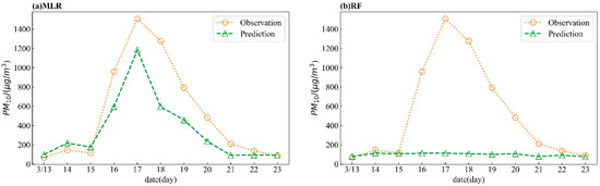
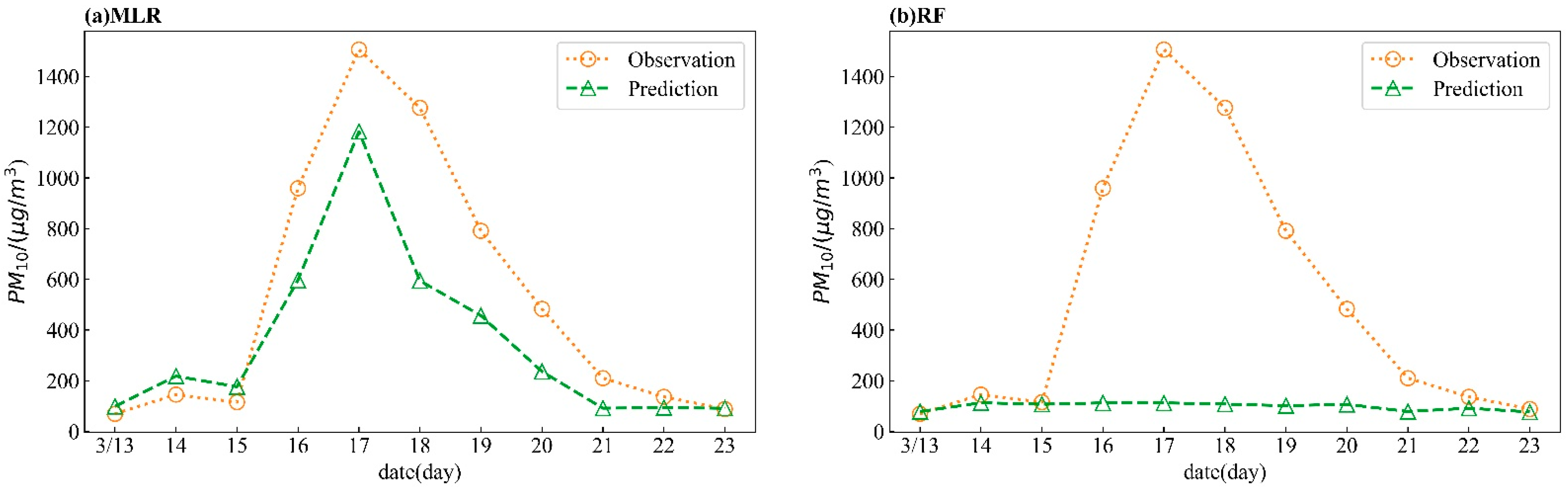
Figure 11.
Comparison between predicted and observed daily mean values of PM10 concentration in Xining City from 13 to 23 March 2021 (a): Multiple Linear Regression, (b): Random Forecast.
On the 16th, large amounts of dust arrived in Xining City, and the observed PM10 concentrations increased sharply, with a daily mean of 959 μg/m3; the AQI grade was at level Ⅵ, and the air quality was significantly polluted with the PM10 concentration exceeding 420 μg/m3. The Multiple Linear Regression algorithm could predict the PM10 concentration on this day more effectively. Although the predicted value was lower than the observed value, which was 596 μg/m3, the AQI grade of the predicted value was also at level Ⅵ with serious pollution, which proved that this method could make effective predictions for such turning weather.
On the 17th, the daily mean of the observed value of PM10 concentration reached the peak, and the predicted value with Multiple Linear Regression also exceeded 1000 μg/m3. There was a consistent corresponding relationship between the observed and predicted values, showing that this method had a satisfactory effect in predicting the maximum value, while the other five machine learning methods did not predict the turning trend and the peak of pollution. From the 18th to the 21st, the predicted value changes were consistent with the observed values, which also decreased day-by-day and the trend was more obvious. The observed value on the 18th was 1276 μg/m3, though the predicted value had been reduced to 594 μg/m3 with large deviation, the AQI grade of the predicted value was still at level Ⅵ.
During the period from 16th to 21st, the prediction effect of the Random Forest was far weak than that of Multiple Linear Regression, and the predicted values were far lower than the observed values. The Random Forest had strong generalization ability and stability, but it was not significant to the missing characteristics. In other words, it was insensitive to outliers. For multidimensional sparse data, the performance of the Random Forest was not ideal. Therefore, in this sudden dust weather, outliers appeared on a large scale, and there was no such feature tree in the training set, so the Random Forest was unable to predict the maximum PM10.
From the 22nd to 23rd, the predicted values were also consistent with the observed values with little deviation using the two methods. In addition, the AQI grades of the predicted values were at level Ⅱ, and the air quality was significantly improved.
As a whole, the Multiple Linear Regression algorithm was not only timely and effective in predicting the PM10 concentration but had great abilities for anticipating the transition period of particle concentration and the appearance date of maximum values in such dust weather.
4.4. Prediction Results of PM10 Concentration in Clean Period
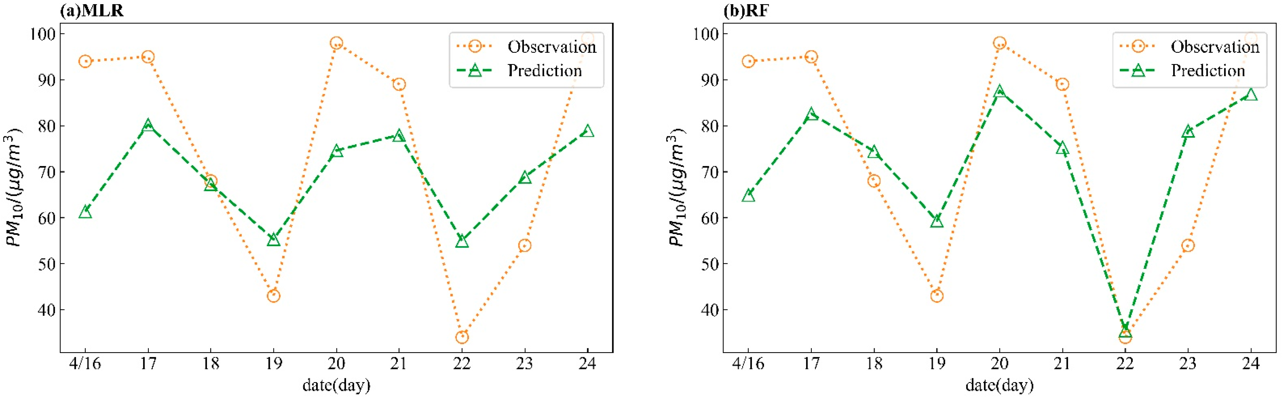
In order to compare with the dust weather, we selected the clean period without dust from the 16th to the 24th of April, 2022 and used Multiple Linear Regression and Random Forecast to predict the PM10 concentration again. As shown in Table 6, the Mean Absolute Error (11 and 14) and Mean Absolute Percentage Error (16% and 20%) of the two methods during the clean period were much lower than that in the dust period; the Index of Agreement and correlation coefficient were also higher. In addition, if the PM10 of Zhangye City was removed from the eigenvalues, the Mean Absolute Error of Random Forest and Multiple Linear Regression increased to 17 and 23, respectively, which indicated that even during the clean period, the PM10 of Zhangye City still played an important role in predicting the PM10 concentration of Xining City.
Table 6.
IA, correlation coefficient, MA, and MP of two methods for predicting PM10 concentration during clean period.
The Index of Agreement of Random Forest was higher, and Mean Absolute Error and Mean Absolute Percentage Error were lower, than Multiple Linear Regression. Compared with Multiple Linear Regression, the predicted values of Random Forest were more consistent with the observed values during the clean period (Figure 12).
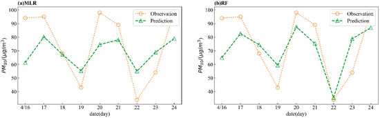
Figure 12.
Comparison between predicted and observed daily mean values of PM10 concentration in Xining City from 16 to 24 April, 2022 (a): Multiple Linear Regression, (b): Random Forecast.
5. Conclusions and Discussion
In view of dust weather affecting the northern Tibetan Plateau from 14 to 20 March 2021, we analyzed the main development mechanisms and explored the leading factors of the dust weather. Using the ECMWF prediction products and PM10 historical observation data with machine learning methods, the trend of PM10 concentration in Xining City during this dust weather was predicted.
- (1)
- The main mechanisms influencing the dust were as follows: The 24-h pressure change was positive when the front intruded on the surface; the convergence of vector winds with a sudden drop in temperature and humidity led by a trough at 700 hPa; a “two troughs and one ridge” weather situation appeared at 500 hPa while the cold advection behind the trough was strong and a cyclone vorticity was formed in the east of Inner Mongolia;
- (2)
- The trajectory of air mass from the Hexi Corridor was the main air mass path influencing Xining City, in this case, since a significant lag in the peak of PM10 concentration appeared in Xining City when compared with Zhangye City;
- (3)
- The Multiple Linear Regression was not only timely and effective in predicting the PM10 concentration but had great abilities for anticipating the transition period of particle concentration and the appearance date of maximum values in such dust weather;
- (4)
- The MA and MP during the clean period were much lower than that during the dust period; the PM10 of Zhangye City as an eigenvalue played an important role in predicting the PM10 of Xining City even during the clean period. In contrast to the dust period, the prediction effect of Random Forest was superior to Multiple Linear Regression during the clean period.
This work was the first time that machine learning methods were applied to dust weather in the northeast city (Xining) of the Tibetan Plateau, which filled the gap of pollution prediction based on artificial intelligence in this area. We selected the eigenvalues from the main weather development mechanisms and found that the PM10 of Zhangye City was the most important eigenvalue. The prediction effect of Random Forest optimized by the Bayesian hyperparameter and other methods were inferior to Multiple Linear Regression for the dust weather, while the Random Forest was the best during clean periods. It indicated that the stability and generalization ability of tree models showed a disadvantage in the prediction of sudden dust weather. In the subsequent work, the machine learning methods need to be further optimized in order to be applied to a wider range of fields.
Author Contributions
Methodology, C.T.; software, C.T. and J.W.; validation, Q.C., C.T. and D.Q.; formal analysis, Q.C.; investigation, L.X.; data curation, L.X. and J.W.; writing—original draft preparation, C.T. and J.W.; writing—review and editing, Q.C.; funding acquisition, L.X., D.Q. and Q.C.; All authors have read and agreed to the published version of the manuscript.
Funding
This research was funded by the Cold Lake Station site monitoring and pilot scientific research project of astronomical big scientific installation (grant number 2019-ZJ-A10), Qinghai Provincial Department of science and technology Planning Project (grant number 2021-SF-141), the Fund of Qinghai Key Laboratory for Disaster Prevention and Reduction (grant number QFZ-2021-M17).
Informed Consent Statement
Not applicable.
Data Availability Statement
All data used to support the findings of this study are available from the first author upon request.
Acknowledgments
We would like to thank the technicians of Institute of Meteorological Science Research of Qinghai Province, Qi Donglin, Quan Chen, for their funding.
Conflicts of Interest
The authors declare that they have no known competing financial interests or personal relationships that could have appeared to influence the work reported in this paper.
References
- Kurosaki, Y.; Mikami, M. Recent frequent dust events and their relation to surface wind in East Asia. Geophys. Res. Lett. 2003, 30, 1736. [Google Scholar] [CrossRef]
- Guo, L.; Fan, B.; Zhang, F.; Jin, Z.; Lin, H. The clustering of severe dust storm occurrence in China from 1958 to 2007. J. Geophys. Res. Atmos. 2018, 123, 8035–8046. [Google Scholar] [CrossRef]
- Shao, Y. Physics and Modelling of Wind Erosion; Kluwer Academic: Dordrecht, The Netherlands, 2009. [Google Scholar]
- De Villiers, M.P.; Heerden, J.V. Dust storms and dust at Abu Dhabi International Airport. Weather 2007, 62, 339–343. [Google Scholar] [CrossRef] [Green Version]
- Sissakian, V.K.; Al-Ansari, N.; Knutsson, S. Sand and dust storm events in Iraq. Nat. Sci. 2013, 5, 1084–1094. [Google Scholar] [CrossRef] [Green Version]
- Stefanski, R.; Sivakumar, M.V.K. Impacts of sand and dust storms on agriculture and potential agricultural applications of a SDSWS. IOP Conf. Ser. Earth Environ. Sci. 2009, 7, 12–16. [Google Scholar] [CrossRef]
- Meo, S.A.; Almutari, F.J.; Abukhalaf, A.A.; Alessa, O.M.; Al-Khlaiwi, T.; Meo, A.S. Sandstorm and its effect on particulate matter PM 2.5, carbon monoxide, ni-trogen dioxide, ozone pollutants and SARS-CoV-2 cases and deaths. Sci. Total Environ. 2021, 795, 148764. [Google Scholar] [CrossRef]
- Goudie, A.S.; Middleton, N.J. Saharan dust storms: Nature and consequences. Earth Sci. Rev. 2001, 56, 179–204. [Google Scholar] [CrossRef]
- Ho, H.M.; Rao, C.Y.; Hsu, H.H.; Chiu, Y.H.; Liue, C.M.; Chaoc, H.J. Characteristics anddeterminants of ambient fungal spores in Hualien Taiwan. Atmos. Environ. 2005, 39, 5839–5850. [Google Scholar] [CrossRef]
- Fang, X.; Han, Y.; Jinghui, M.A.; Song, L.; Yang, S.; Zhang, X. Dust storms and loess accumulation on the Tibetan Plateau: A case study of dust event on 4 March 2003 in Lhasa. Sci. Bull. 2004, 49, 953–960. [Google Scholar] [CrossRef]
- Peng, S.; Li, Y.; Liu, H.; Han, Q.; Zhang, X.; Feng, Z.; Chen, D.; Ye, W.; Zhang, Y. Formation and evolution of mountainous aeolian sediments in the northern Tibet Plateau and their links to the Asian winter monsoon and westerlies since the Last Glacial Maximum. Prog. Phys. Geogr. 2021, 46, 43–60. [Google Scholar] [CrossRef]
- Shao, Y. Northeast Asian dust storms: Real-time numerical prediction and validation. J. Geophys. Res. 2003, 108, AAC 3-1. [Google Scholar] [CrossRef] [Green Version]
- Zhao, Y.; Li, H.J.; Huang, A.N.; He, Q.; Huo, W.; Wang, M. Relationship between thermal anomalies in Tibetan Plateau and summer dust storm frequency over Tarim Basin, China. J. Arid Land 2013, 5, 25–31. [Google Scholar] [CrossRef] [Green Version]
- Sun, Z.B.; Wang, H.; Guo, C.; Wu, J.; Cheng, T.; Li, Z.-M. Barrier effect of terrain on cold air and return flow of dust air masses. Atmos. Res. 2019, 220, 81–91. [Google Scholar]
- Wang, T.H.; Tang, J.Y.; Sun, M.X.; Liu, X.; Huang, Y.; Huang, J.; Han, Y.; Cheng, Y.; Huang, Z.; Li, J. Identifying a transport mechanism of dust aerosols over South Asia to the Tibetan Plateau: A case study. Sci. Total Environ. 2021, 758, 143714. [Google Scholar] [CrossRef] [PubMed]
- Zhao, J.; Ma, X.; Wu, S.; Sha, T. Dust emission and transport in Northwest China: WRF-Chem simulation and comparisons with multi-sensor observations. Atmos. Res. 2020, 241, 104978. [Google Scholar] [CrossRef]
- Singh, C.; Singh, S.K.; Chauhan, P.; Budakoti, S. Simulation of an extreme dust episode using WRF-CHEM based on optimal ensemble approach. Atmos. Res. 2020, 249, 105296. [Google Scholar] [CrossRef]
- Li, J.; Man, S.W.; Lee, K.H.; Nichol, J.; Chan, P.W. Review of dust storm detection algorithms for multispectral satellite sensors. Atmos. Res. 2021, 250, 105398. [Google Scholar] [CrossRef]
- Ranjan, A.K.; Patra, A.K.; Gorai, A.K. A Review on Estimation of Particulate Matter from Satellite-Based Aerosol Optical Depth: Data, Methods, and Challenges. J. Atmos. Sci. 2021, 57, 679–699. [Google Scholar] [CrossRef]
- Qing, X.; Zheng, S. A New Method for Initialising the K-Means Clustering Algorithm; IEEE Computer Society: Washington, DC, USA, 2009. [Google Scholar]
- Lin, P.; Hu, G.; Li, C.; Li, L.; Xiao, Y.; Tse, K.T.; Kwok, K.C. Machine learning-based prediction of crosswind vibrations of rectangular cylinders. J. Wind Eng. Ind. Aerodyn. 2021, 211, 104549. [Google Scholar] [CrossRef]
- Xi, X.; Zhao, W.; Rui, X.; Wang, Y.; Bai, X.; Yin, W.; Don, J. A comprehensive evaluation of air pollution prediction improvement by a machine learning method. In Proceedings of the 2015 IEEE International Conference on Service Operations And Logistics, And Informatics (SOLI), Hammamet, Tunisia, 15–17 November 2015; pp. 176–181. [Google Scholar] [CrossRef]
- Tao, J. Elevation-dependent temperature change in the Qinghai-Xizang Plateau grassland during the past decade. Theor. Appl. Climatol. 2014, 117, 61–71. [Google Scholar] [CrossRef]
- Al Murayziq, T.S.; Kapetanakis, S.; Petridis, M. Intelligent Signal Processing for Dust Storm Prediction Using Ensemble Case-Based Reasoning. In Proceedings of the 2017 IEEE 29th International Conference on Tools with Artificial Intelligence (ICTAI), Boston, MA, USA, 6–8 November 2017; pp. 1267–1271. [Google Scholar] [CrossRef]
- Kaimian, H.; Li, Q.; Wu, C.; Qi, Y.; Mo, Y.; Chen, G.; Zhang, X.; Sachdeva, S. Evaluation of Different Machine Learning Approaches in Forecasting PM2.5 Mass Concentrations. Aerosol Air Qual. Res. 2019, 19, 1400–1410. [Google Scholar] [CrossRef] [Green Version]
- Yang, G.; Lee, H.M.; Lee, G. A Hybrid Deep Learning Model to Forecast Particulate Matter Concentration Levels in Seoul, South Korea. Atmosphere 2020, 11, 348. [Google Scholar] [CrossRef] [Green Version]
- Feng, X.; Li, Q.; Zhu, Y.; Hou, J.; Jin, L.; Wang, J. Artificial neural networks forecasting of PM2.5 pollution using air mass trajectory based geographic model and wavelet transformation. Atmos. Environ. 2015, 107, 118–128. [Google Scholar] [CrossRef]
- Huang, L.; Zhang, C.; Bi, J. Development of land use regression models for PM2.5, SO2, NO2 and O3 in Nanjing, China. Environ. Res. 2017, 158, 542–552. [Google Scholar] [CrossRef] [PubMed]
- Perez, P.; Menares, C. Forecasting of hourly PM2.5 in south-west zone in Santiago de Chile. Aerosol Air Qual. Res. 2018, 18, 2666–2679. [Google Scholar] [CrossRef] [Green Version]
- Li, J.; Shao, X.; Zhao, H. An Online Method Based on Random Forest for Air Pollutant Concentration Forecasting. In Proceedings of the 37th China Control Conference, Wuhan, China, 25–27 July 2018. [Google Scholar]
- Jiang, F.; Qiao, Y.; Jiang, X.; Tian, T. MultiStep Ahead Forecasting for Hourly PM10 and PM2.5 Based on Two-Stage Decomposition Embedded Sample Entropy and Group Teacher Optimization Algorithm. Atmosphere 2021, 12, 64. [Google Scholar] [CrossRef]
- Park, S.; Kim, M.; Kim, M.; Namgung, H.G.; Kim, K.T.; Cho, K.H.; Kwon, S.B. Predicting PM 10 concentration in Seoul metropolitan subway stations using artifificial neural network (ANN). J. Hazard. Mater. 2018, 341, 75–82. [Google Scholar] [CrossRef]
- Yumimoto, K.; Murakami, H.; Tanaka, T.Y.; Sekiyama, T.T.; Ogi, A.; Maki, T. Forecasting of Asian dust storm that occurred on May 10–13, 2011, using an ensemble-based data assimilation system. J. Part. 2016, 28, 121–130. [Google Scholar] [CrossRef]
- Xu, Y.; Xu, E. ARIMA and Multiple Regression Additive Models for PM2.5 Based on Linear Interpolation. In Proceedings of the 2020 In-ternational Conference on Big Data & Artificial Intelligence & Software Engineering (ICBASE), Bangkok, Thailand, 30 October–1 November 2020; pp. 266–269. [Google Scholar] [CrossRef]
- Chen, J.; Wang, J. Prediction of PM2.5 Concentration Based on Multiple Linear Regression. In Proceedings of the 2019 International Conference on Smart Grid and Electrical Automation (ICSGEA), Xiangtan, China, 10–11 August 2019. [Google Scholar]
- Sinnott, R.O.; Guan, Z. Prediction of Air Pollution through Machine Learning Approaches on the Cloud. In Proceedings of the 2018 IEEE/ACM 5th International Conference on Big Data Computing Applications and Technologies (BDCAT), Zurich, Switzerland, 17–20 December 2018. [Google Scholar]
- Vlachogiannis, D.; Sfetsos, A. Time Series Forecasting of Hourly PM10 Values: Model Intercomparison and the Development of Localized Linear Approaches. In Air Pollution; WIT Press: Southampton, UK, 2006. [Google Scholar]
- Abraham, A.; Pedregosa, F.; Eickenberg, M.; Gervais, P.; Mueller, A.; Kossaifi, J.; Gramfort, A.; Thirion, B.; Varoquaux, G. Machine Learning for Neuroimaging with Scikit-Learn. Front. Neuroinform. 2013, 8, 14. [Google Scholar] [CrossRef] [Green Version]
- Tran, M.K.; Panchal, S.; Chauhan, V.; Brahmbhatt, N.; Mevawalla, A.; Fraser, R.; Fowler, M. Python-based scikit-learn machine learning models for thermal and electrical performance prediction of high-capacity lithium-ion battery. Int. J. Energy Res. 2021, 46, 786–794. [Google Scholar] [CrossRef]
- Sousa, S.; Martins, F.G.; Alvim-Ferraz, M.; Pereira, M.C. Multiple linear regression and artificial neural networks based on principal components to predict ozone concentrations. Environ. Model. Softw. 2007, 22, 97–103. [Google Scholar] [CrossRef]
- Albergaria, J.T.; Martins, F.G.; Alvim-Ferraz, M.; Delerue-Matos, C. Multiple Linear Regression and Artificial Neural Networks to Predict Time and Efficiency of Soil Vapor Extraction. Water Air Soil Pollut. 2014, 225, 1–9. [Google Scholar] [CrossRef] [Green Version]
- Baczek, T.; Wiczling, P.; Marsza, M.; Heyden, Y.V.; Kaliszan, R. Prediction of peptide retention at different HPLC conditions from multiple linear regression models. J. Proteome Res. 2005, 4, 555–563. [Google Scholar] [CrossRef] [PubMed]
- Wessel, M.D.; Jurs, P.C. Prediction of Reduced Ion Mobility Constants from Structural Information Using Multiple Linear Regression Analysis and Computational Neural Networks. Anal. Chem. 1994, 66, 2480–2487. [Google Scholar] [CrossRef]
- Breiman, L.; Friedman, J.H.; Olshen, R.A.; Stone, C.J. Classification and Regression Trees; Wadsworth Inc.: Belmont, CA, USA, 1984. [Google Scholar]
- Hou, W.; Li, Z.; Zhang, Y.; Xu, H.; Zhang, Y.; Li, K.; Li, D.; Wei, P.; Ma, Y. Using support vector regression to predict PM10 and PM2.5. IOP Conf. Ser. Earth Environ. Sci. 2014, 17, 012268. [Google Scholar]
- Keller, J.M.; Gray, M.R.; Givens, J.A. A fuzzy K-nearest neighbor algorithm. IEEE Trans. Syst. Man Cybern. 2012, 4, 580–585. [Google Scholar] [CrossRef]
- Maltamo, M.; Kangas, A. Methods based on k-nearest neighbor regression in the prediction of basal area diameter distribution. Can. J. For. Res. 2011, 28, 1107–1115. [Google Scholar] [CrossRef]
- Chan, C.W.; Paelinckx, D. Evaluation of Random Forest and Adaboost tree-based ensemble classification and spectral band selection for ecotope mapping using airborne hyperspectral imagery. Remote Sens. Environ. 2008, 112, 2999–3011. [Google Scholar] [CrossRef]
- Xia, L.; Bai, R. Freight Vehicle Travel Time Prediction Using Gradient Boosting Regression Tree. In Proceedings of the IEEE International Conference on Machine Learning & Applications, Anaheim, CA, USA, 18–20 December 2016. [Google Scholar]
- Sousa, P.M.; Trigo, R.M.; Barriopedro, D.; Soares, P.M.; Ramos, A.M.; Liberato, M.L. Responses of European precipitation distributions and regimes to different blocking locations. Clim. Dyn. 2016, 48, 1–20. [Google Scholar] [CrossRef] [Green Version]
- GB 3095-2012; Ambient Air Quality Standards. China Environmental Science Press: Beijing, China, 2012.
- GB/t20480-2017; Classification of Sand and Dust Weather. China National Standardization Administration Committee: Beijing, China, 2017.
- Zhang, P.; Wu, H.N.; Chen, R.P.; Chan, T.H. Hybrid meta-heuristic and machine learning algorithms for tunneling-induced settlement prediction: A comparative study. Tunn. Undergr. Space Technol. 2020, 99, 103383. [Google Scholar] [CrossRef]
- Wang, S.; Zhuang, J.; Zheng, J.; Fan, H.; Kong, J.; Zhan, J. Application of Bayesian hyperparameter optimized random forest and XGBoost model for landslide susceptibility mapping. Front. Earth Sci. 2021, 9, 617. [Google Scholar] [CrossRef]

Publisher’s Note: MDPI stays neutral with regard to jurisdictional claims in published maps and institutional affiliations. |
© 2022 by the authors. Licensee MDPI, Basel, Switzerland. This article is an open access article distributed under the terms and conditions of the Creative Commons Attribution (CC BY) license (https://creativecommons.org/licenses/by/4.0/).