Article

Predicting Meteorological Variables on Local Level with SARIMA, LSTM and Hybrid Techniques

by
Antonios Parasyris
*,
George Alexandrakis
,
Georgios V. Kozyrakis
,
Katerina Spanoudaki
and
Nikolaos A. Kampanis
Foundation for Research and Technology-Hellas, Institute of Applied and Computational Mathematics, 70013 Heraklion, Greece
*
Author to whom correspondence should be addressed.
Atmosphere 2022, 13(6), 878; https://doi.org/10.3390/atmos13060878
Submission received: 7 May 2022 / Revised: 25 May 2022 / Accepted: 27 May 2022 / Published: 28 May 2022

Abstract

:
The choice of holiday destinations is highly depended on climate considerations. Nowadays, since the effects of the climate crisis are being increasingly felt, the need for accurate weather and climate services for hotels is crucial. Such a service could be beneficial for both the future planning of tourists’ activities and destinations and for hotel managers as it could help in decision making about the planning and expansion of the touristic season, due to a prediction of higher temperatures for a longer time span, thus causing increased revenue for companies in the local touristic sector. The aim of this work is to calculate predictions on meteorological variables using statistical techniques as well as artificial intelligence (AI) for a specific area of interest utilising data from an in situ meteorological station, and to produce valuable and reliable localised predictions with the most cost-effective method possible. This investigation will answer the question of the most suitable prediction method for time series data from a single meteorological station that is deployed in a specific location; in our case, in a hotel in the northern area of Crete, Greece. The temporal resolution of the measurements used was 3 h and the forecast horizon considered here was up to 2 days. As prediction techniques, seasonal autoregressive integrated moving average (SARIMA), AI techniques like the long short-term memory (LSTM) neural network and hybrid combinations of the two are used. Multiple meteorological variables are considered as input for the LSTM and hybrid methodologies, like temperature, relative humidity, atmospheric pressure and wind speed, unlike the SARIMA that has a single variable. Variables of interest are divided into those that present seasonality and patterns, such as temperature and humidity, and those that are more stochastic with no known seasonality and patterns, such as wind speed and direction. Two benchmark techniques are used for comparison and quantification of the added predictive ability, namely the climatological forecast and the persistence model, which shows a considerable amount of improvement over the naive prediction methods, especially in the 1-day forecasts. The results indicate that the examined hybrid methodology performs best at temperature and wind speed forecasts, closely followed by the SARIMA, whereas LSTM performs better overall at the humidity forecast, even after the correction of the hybrid to the SARIMA model. Lastly, different hybrid methodologies are discussed and introduced for further improvement of meteorological predictions.

1. Introduction

Identifying and predicting climatic characteristics can have a great impact on many facets of everyday human life and is known to affect the mood and the choice of everyday activities. For applications like photovoltaic and wind energy prediction, climate change scenario forecasting, extreme events, etc., various techniques have been used; see for example [1], where the authors review the abundant literature of research papers related to machine learning methods and numerical weather prediction based on the application.
Weather prediction, the application in the scope of our research, is associated with tourists’ satisfaction based on the climatic conditions. For the tourism industry, weather is a key factor [2]. The choice of a holiday destination is highly dependent on climate considerations, and so, as the climate crisis repercussions are being increasingly felt, the need for meteorological prediction services for hotels becomes a necessity, both for tourists and hotel managers. Existing applications of weather forecasting that involve in situ information from an MS aim at current comfort indices evaluation and heritage risk analysis, e.g., [3], but do not consider simplified weather forecasts using accurate in situ real-time datasets. This service directed at touristic comfort and satisfaction based on the weather conditions is being overlooked, and the usual source of information that many hotels offer involve private meteorological companies like Accuweather, WeatherNet, Meteo, etc. [4]. These services typically use models with limited accuracy and low spatial resolution, may experience downtimes and might even require subscription fees from the tourist for more premium and robust functionalities, something that can have a negative impact on a tourist’s experience. Zeng et al. [5] used random forests to predict solar radiation with a high-density meteorological station grid; however, that cannot be utilized here as the plurality of data observation locations and the lack of accuracy make it a nonviable option for operational purposes. The decision as to which predictors can be exploited and used with these kinds of datasets for accurate weather prediction is identified as the research gap that this paper addresses.
Our research develops and compares prediction methods that are suitable to be applied on a small and affordable scale, such that even a small-scale hotel can afford the installation and maintenance for the forecasting system locally, without dependence on expensive models and subscription fees for forecasting services. Thus, the problem involves time series prediction, which poses a challenging problem on its own [6], but also includes meteorological variables, which tend to exhibit chaotic behaviours and cannot be easily forecasted with a single point source time series [7]. Additionally, in statistical forecasting approaches, the huge downside is that stochasticity is present in the sense that there is not one single theoretical model that can outperform all methods in any given situation; see for example [8,9]. Each method’s performance is heavily reliant on the given dataset, nature of the problem, stationarity of the data, noisy data, trend, cyclicity of data, etc. This also gives rise to a very active field of hybrid methodologies and new techniques being invented, that better suit some problems whilst underperform in others. For that reason, and to address the problem of predicting short-term meteorological variables, we will test and employ different techniques that are proposed in the literature for our given dataset and variables.
First and foremost, the most used and researched methodology for time series forecasting is the autoregressive integrated moving average (ARIMA) model [10,11], where there exists abundant literature to support the use for short time prediction [6], even for meteorological variables that tend to exhibit chaotic behaviour [12,13]. The work of Jayawardena et al. [14] addressed the prediction of chaotic hydrometeorological time series by first applying nonlinear noise reduction techniques and then predicting using ARIMA compared with other deterministic models. Paulescu et al. [15] described the prediction of solar radiation using ARIMA models, where good agreement, even for the high accuracy needed for photovoltaic systems’ energy production, was found. Additionally, Paulescu et al. [15] noted that as the prediction window is enlarged (more than a day), the errors accumulate so much that the resulting accuracy is reduced significantly. Moreover, first order differencing in ARIMA analysis of climate datasets is necessary to remove the non-stationarity and hence improve the accuracy of the predictions [15]. If longer time series with multiple periodicities are available, seasonal ARIMA (SARIMA) models are better suited and show a better fit [6]. The short-term hydrometeorological variables’ prediction with multiple measurement stations in the coastal zone was studied by Tylkowski et al. [16], where the SARIMA method has provided reliable information to help in environmental planning and decision making, based on monthly averaged predictions for air temperature, total atmospheric precipitation and average sea level.
When datasets comprising nonlinear time series are available consistently for many years, artificial neural networks (NN) are better suited for forecasting [17]. NN fall under the broader category of machine learning (ML) techniques and possess the ability to improve automatically through experience and by the use of data, as can be found in ML textbooks, see, e.g., [18]. NN are seen as a part of artificial intelligence (AI), where the general idea is to use sample data known as a “training dataset” to make predictions or decisions without being explicitly programmed to do so. These have many applications like email filtering, computer vision, data mining and optimization and are powerful nonlinear regression techniques inspired by theories of how the brain works [18]. These methods have been successfully implemented for hydrological time series forecasting, see, e.g., [19]. Artificial NN with various input data lengths were compared and proven superior to the autoregressive models in a hydrological time series application in [20]. Multilayer perceptron (MLP) NN is well suited to predict other hydrological variables like the daily streamflow, as demonstrated in [21].
ARIMA and its seasonal counterpart SARIMA were found in numerous studies e.g., [6,12,13,22,23,24] to be well suited to tackle problems like the 1–2 day ahead prediction of some weather variables, such as air temperature, humidity, solar radiation, wind speed, etc. In order to be useful in more applications with larger prediction horizons and more chaotic weather variables, combinations and hybridizations based on ML and SARIMA are suggested by authors e.g., [24,25,26,27,28,29] and the references therein. Applications with hydrological time series forecasting with hybrid techniques can be found for example in Di et al. [19], where the hybrid techniques with combined models outperform the conventional single model methodologies. The task of creating robust and reliable hybrid techniques that improve the accuracy of time series prediction algorithms is perhaps the most researched question in the field and it will be discussed more in depth in the methodology and discussion sections. Another aspect of this research is to be able to accurately depict weather and climate phenomena locally near a point of interest. The data sources will be discussed in the data section below.
The paper is structured as follows: The prediction methods that will be considered are introduced and discussed in the Materials and Methods section, namely the more classical time series prediction of the SARIMA method and artificial intelligence techniques such as the LSTM neural networks and hybrid combinations as indicated by the literature. Next, we introduce our approach on a hybrid method, which is implemented for the examined dataset. In the last sections, we compare the results of the three models, for three different meteorological variables and two short-term prediction horizons. Finally, we conclude with our preferences and comments on other methods and different hybridization techniques that could further assist and improve the predictions.

2. Materials and Methods

In this section, we will briefly describe the methods we will utilize regarding the short-term forecasting of the weather conditions at a location of interest. We will also describe the details of each methodology that were essential for its implementation.

2.1. Data

For the accurate depiction of the weather near the point of interest, which for this application is a hotel in Crete, a meteorological station (MS) has been installed in place and maintained by the Coastal & Marine Research Laboratory (CMRL) https://crl.iacm.forth.gr/en/ (accessed on 1 May 2022) and is able to provide a continuous feed of data. The location of the hotel in which the station has been installed is chosen as a representative example of the northern area of Crete, a highly significant socioeconomic centre which is heavily financially dependent on the touristic sector. More specifically, the MS is installed on an open field on a rooftop in an optimized position in order to assess the microclimate of the area, as seen in Figure 1. The area is also selected with respect to its representativeness of the northern Cretan microclimate.
The MS records in a minutely temporal resolution, so that 3-h averages or maximum–minimum values have been obtained. The variables used here as inputs or outputs include combinations of the maximum mean air temperature (Celsius), minimum mean relative humidity (%), mean barometric pressure, total precipitation (mm) and the average wind speed (m/s) and direction. The MS has been fully operational since 2019 and therefore the amount of data were deemed insufficient for a fair comparison of the SARIMA, the LSTM and the hybrid to be carried out. To circumvent this and achieve a methodological comparison based on the results, another dataset was provided by the Hellenic National Meteorological Service (http://www.emy.gr/emy/el/services/paroxi-ipiresion-elefthera-dedomena accessed on 9 December 2021) which comprised of measurements from an MS similar to the one installed by the authors, located in a close-by area with similar climatic characteristics. This dataset comprised of the same variables, measured at a 3-h temporal resolution, spanning the years 1975–2004. In this way, the methods investigated could be fairly compared and a proof of concept could be made which can be applied on the in situ data from our MS in the future. The training of all methods will be carried out in a fraction of this dataset, as will be discussed in the methodology section later on.
The selection of these variables was based on studies that associate tourism applications to meteorological variables that can be found, for example, in [30,31] and, more specifically in the case of Greece where tourism depends on summertime beach activities, in [2] and the references therein.

2.2. ARIMA Methodology

The methodology for fitting an ARIMA model into our data can be easily handled in R software by the “auto.arima” function [32,33]. It utilizes the Box–Jenkins algorithm [32,33] to fit an ARIMA model into the training dataset. To do that, it searches for a triplet [P,D,Q] that corresponds to [terms of autoregression AR, degree of differencing, terms of moving average (MA)], respectively, which will make the model fit the given training dataset with a minimized error. After the optimum triplet has been found, the model can make predictions of a specified length using the “predict” function embedded in R, and can also compare the dataset on which it has been trained with the predicted values that the model would output. This is called herein the ARIMA residual, or simply a residual. It is worth mentioning that the ARIMA model fitted here is one dimensional, that means that for every prediction made, only the variable of interest is considered as an input of the model. This may negatively affect the accuracy, but it significantly improves the computational time and simplicity of the method, which can be used effectively in automatic mode (see, e.g., [32]) without requiring significant expert knowledge, which is an advantage over the other techniques.
One question that this paper addresses is the relevancy and the usefulness of each predictor for the application at hand. For that reason, the next section briefly introduces the artificial neural networks (ANN) as a predictor and later we will compare results from both methods as well as hybrid combinations of them.

2.3. Artificial Neural Networks (ANN)–LSTMs

Neural networks are known to perform very well in noisier and nonlinear data where other methods fail, in contrast with the ARIMA method that is capable of handling linear time series prediction. One issue faced for long time series is that even small errors can propagate and result in failure of the convergence of the model [34]. Thus, the so-called long short-term memory (LSTM) neural networks have been used, which are a special category of recurrent ANN, and have presented to be the most suited of all the neural networks for time series prediction [34,35]. The suitability of the LSTM to forecast long time series is the result of their ability to remember using information that a simple NN cannot by using long-term memory cells, and at the same time, to solve vanishing gradient issues where the standard recurrent neural networks hinder performance. A more detailed description of the LSTM cell operation and differences with a standard NN cell can be found in [36], in which relevant algorithmic forms of the model are given in their figures, and the superiority of LSTMs for a hydrology example is demonstrated. Additionally, in a comparison of ARIMA and LSTM applied to wind speed, [37] showed that the LSTM can perform better in large datasets, but for smaller datasets, the ARIMA technique might outperform the LSTM due to the lack of training and pattern learning of the specific NN architecture.
For each of the LSTM neural networks shown in the results section, we conducted a grid search of parameters and architectures to determine a near optimal configuration. For some networks, the use of an SGD (stochastic gradient descent) [38] optimizer achieves better results (when standard momentum = 0.9), whereas in other examples, the use of Adam optimizers is best [39]. The learning rate was set to the standard 0.01, with an update of 0.005 and a “patience” parameter equal to 5, meaning that the algorithm updates the learning rate every 5 epochs that the loss does not improve.
Usually, we propose 40 units in each layer but some tests had better results with 100 units, with the deterioration of the computational time. Most often we obtained good accuracy with one input layer, two hidden LSTM layers and one dense as output layer. All layers use a rectified linear unit (ReLU) activation function, as tests with others showed deterioration in accuracy. The epochs of training ranged from 20 to 60, and a combination of the grid search and the validation error helped us to avoid over fitting. Additionally, a callback that monitored the loss and had a patience of 5 epochs reduced the learning rate starting from 0.01 by a factor of 0.005. The neural network was designed by having a week of previous data as input (56 3-h samples) and either a 1-day or 2-day ahead forecast horizon (8 or 16 3-h samples). As loss error, the mean squared error (MSE) was picked, whereas for comparison between the methods and easier translation to the real-world problem, the mean absolute error (MAE) was employed, which has the same units as the prediction variable (Celsius for temperature, % for relative humidity and m/s for wind speed). For each day or 2-day ahead in the test set, a prediction was made and compared with the actual data which was not included in the training process of any algorithm. This was achieved by taking the absolute value of their difference and then the mean for each day. Then, another average over all the days of the test set was corresponded to the value shown in Table 1 for the three variables of interest, namely temperature, humidity and wind speed. We also used all the other correlated variables with the prediction variable in each run, and they were included as features. For example, for temperature prediction, humidity, wind speed and pressure were used, and similarly for the other two networks we created for humidity and wind speed. Additionally, two sine and cosine waves were added as features, with frequencies 2 ∗ pi ∗ (D-Y%) where D-Y% was either the daily percentage of hours passed within a day, or the yearly percentage of days passed within the year. This way, the oscillation that shows the daily and yearly frequency was also used as a feature for the LSTM. The addition of both sine and cosine waves is preferred since using just a sine for the daily cycle, for example, takes the same value twice in each day, whereas a combination of sine and cosine as two separate features uniquely specifies each time of the day/year cycle. In conclusion, each LSTM had eight features (four weather related and four sine–cosine waves for the daily/yearly cycle).
For the introduction of hybrid methodologies in the next section, the assumption is that ARIMA residuals exhibit this kind of nonlinear noisier behaviour, and thus a combination of the two methodologies in which neural networks are used to predict the future ARIMA residual and are added to the ARIMA forecast is suggested. This is expected to result in a predictor–corrector method that can in principle improve accuracy.

2.4. ARIMA–LSTM Hybrid Methodology

As mentioned in the introduction, a significant amount of research is spent on exploring new hybrid methods in an attempt to increase accuracy, but this is a problem-dependent question. On similar applications, Saba et al. [28] worked towards a hybrid method for weather prediction where they averaged multilayer perceptron and radial basis function neural network outputs and succeeded in reducing the error with the simplification that their output was just a decision between rainy or dry weather. This is much simpler than actually predicting multiple time steps of values of every single variable, and can achieve higher accuracy due to this simplification. It is also worth mentioning that the authors used a relatively small dataset of 5 years of data for both training and testing, which could be a reason they had to resort to this kind of simplified prediction.
The hybrid method that we will use is inspired by the work of Deng et al. [29] where ARIMA is used as a primary predictor, and subsequently an NN is used to correct the result by predicting the residual with an LSTM. As discussed before, the same eight features are used here for the LSTM, in addition to the residuals of each predicted variable. All tests were performed in R using “keras” under “tensorflow”.

2.5. Benchmarking

To quantify the increase in predictive capability of the methods, a comparison of the best performer from the LSTM, SARIMA and the hybrid methods with two benchmark prediction techniques has been made [40]. The first technique is the climatological benchmark, which represents the average of all measurements in the training set for each 3-h interval for each day. Hence, we obtain a baseline of what the weather will be like if it followed exactly the average of the previous years. The second prediction is the naive persistence technique, which substitutes the last known measurements as predictions, essentially hypothesizing that the weather conditions will repeat exactly as they have in the previous day/days.

3. Results

We split the presentation of the results into two categories, (a) predictions of temperature and humidity, which are easier to achieve and (b) the more chaotic wind forecasts. The computational time for each NN epoch was on average about 3 min (depending on the units used), so for a 40 epoch LSTM with 40 units at each of two hidden LSTM layers, which was a common configuration we used, 2 h were spent for training each LSTM. On the other hand, for the SARIMA fit we reported an average time of 3 min for each fit, which is significantly faster than any of the neural networks. We note here that for the 1-day or the 2-day forecast, the same SARIMA model is used, so one does not have to compute again the SARIMA fit for bigger prediction horizons, although the accuracy is known to significantly deteriorate as bigger prediction horizons are considered [17]. For the computational time of the hybrid, as it is a combination of the two techniques, we have a cumulative computational time, but frequently less epochs were used for the hybrid, so in most runs it was faster than the LSTM, but significantly slower than the SARIMA.

3.1. Temperature and Humidity Forecast

For the 1-day prediction, we fitted the ARIMA model with a seasonal component (SARIMA) for our 3-h temperature data, which was 70% of the total data (out of 61,363 total measurements, 42,954 were used with the SARIMA fitting) which gave the ARIMA (1, 0, 2) (2, 1, 2) [8] result where 8 is the time series frequency (daily), and (2,1,2) are the [P,D,Q] that correspond to the seasonal component amount of terms, again for [terms of autoregression AR, degree of differencing, terms of moving Average (MA)].
To obtain a fair comparison with the standard LSTM model, a standard 70% training, 15% validation and 15% training split was employed at every instance where a neural network was needed. Additionally, a scaling in the range of (0, 1) of all the variables separately before being inputted into the algorithms was performed. After the predictions were given by the models, an inverse transform computed the final outcomes in the correct range which are shown in the figures below. To get rid of the stochasticity of the results that is inherent to neural networks, each mean absolute error (MAE) presented in Table 1 acted as a representative through means of averaging, of multiple runs with the same parameters as well as many days over the test set. Table 1 shows the MAE of the predictions in 1-day and 2-day horizons, in which we observe how small the error of the hybrid and SARIMA model is, compared to what we accomplished with the LSTM, except in the case of humidity, where the LSTM shows an improvement from both methods.
Furthermore, a small reduction of the error is achieved through hybridization, which is normal since this depends significantly on the SARIMA fit and the algorithm performs an improvement upon the residual errors of the SARIMA. Additionally, we note that as the prediction window increases to 2 days, the gap between the methods becomes smaller, especially in the case of wind speed prediction. In the case of humidity, the error reduction of the hybrid does not make it better than the LSTM, which is 2% better in the 2-day predictions. For the temperature predictions, the hybrid shows the lowest average MAEs, but is very closely followed by the SARIMA.
The predictive ability is demonstrated and quantified by the comparison of the methods with the two benchmark methods, namely the climatological and the naive persistence method. For the 1-day temperature prediction a 44% improvement of the best method (hybrid) in comparison to the climatological and a 56% improvement over the persistence model is reported. Additionally, for 1-day humidity we find a 16% and 48% improvement of the LSTM over the climatological and persistence, respectively. Lastly, the wind speed where the hybrid had the least errors, a 19% and a 52% error improvement of the two benchmarks for the first day is reported, and similarly a 6% and a 36% for the 2-day predictions. The overall worst performers compared to the benchmarks were at 2-day temperature and humidity, where the best predictors had a 5% and 11% over the climatological benchmark, and in the humidity case, the climatological benchmark even outperformed some of the methods. Overall, the climatological benchmark was the best out of the two benchmarks, partly explained due to the rapid change of weather variables (especially wind speed) in a 1–2-day horizon, and the non-repeatability of weather phenomena. On the other hand, the climatological benchmark included many years of averages for each of the 3-h intervals and each one of the days, and since the climate is considered temperate in Crete, it is reasonable that it provided better results as a benchmark.
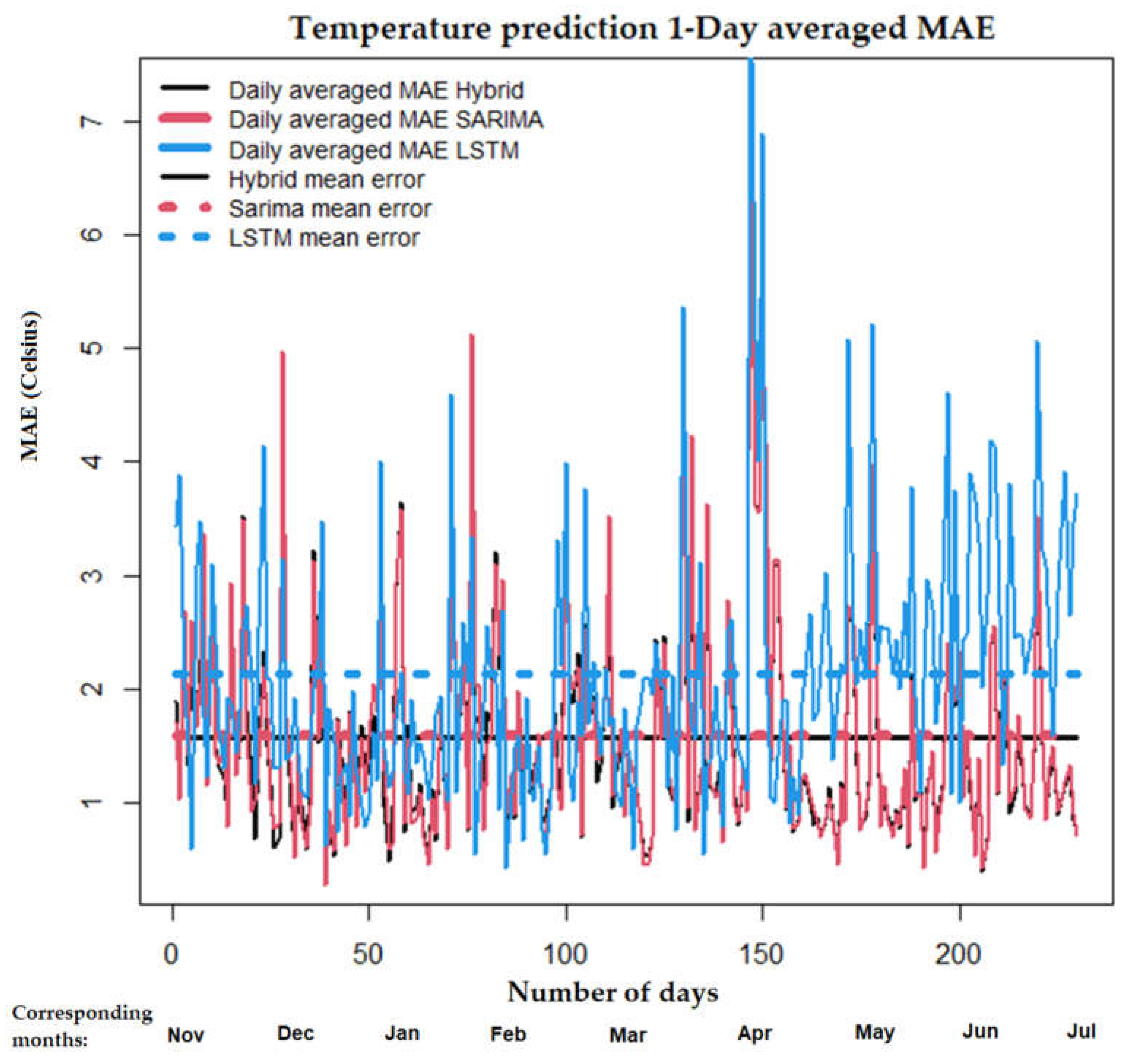
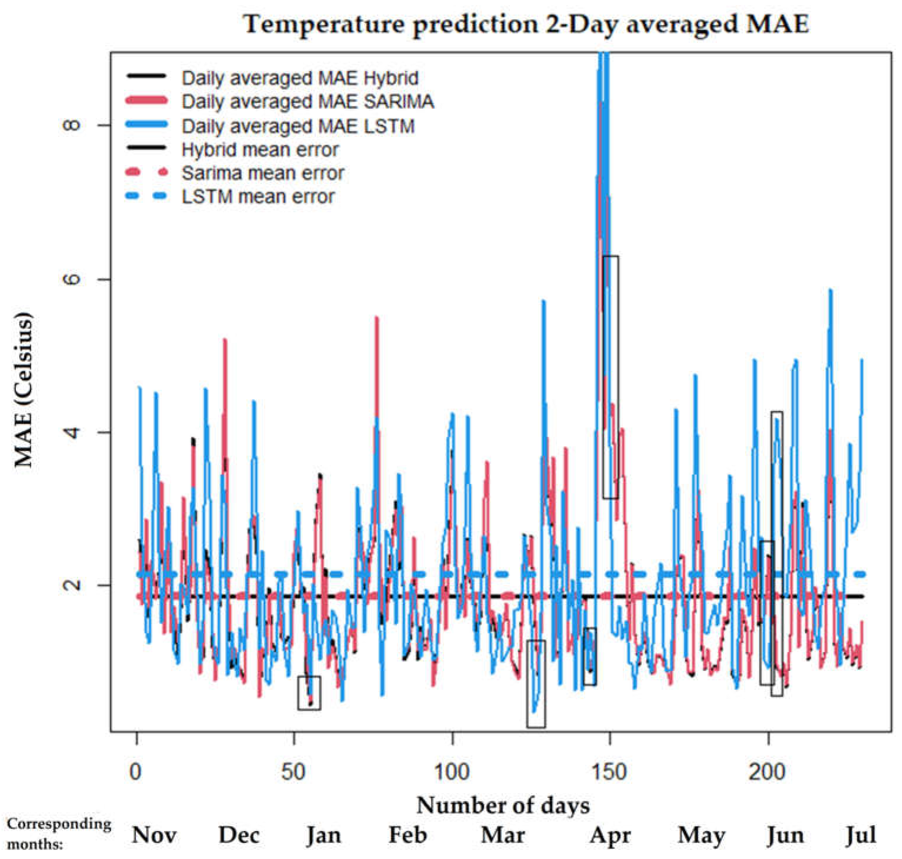
The daily averaged MAE for the 1- and 2-day prediction horizon is presented in Figure 2 and Figure 3, focused on the temperature in this section, for 230 days of the test set. We present MAEs for the three different methods which are colour-coded, and with the same colour and dashed lines we plot the average of all the days in the test set as calculated in Table 1. As we can see in Figure 2 the lower values of the hybrid are followed closely by the SARIMA, and the worst method for the 2-day prediction is the LSTM. Another useful takeaway from Figure 2 and Figure 3 is that there is a significant error at the 150-day mark (April), and since our test set begins in November, all the first 150 days have lower values of true temperature, whereas after April, higher temperatures are consistently observed in the test dataset. The LSTM seems to have larger errors than the SARIMA and the hybrid in those last two months (May and June) compared to the previous winter/spring months.
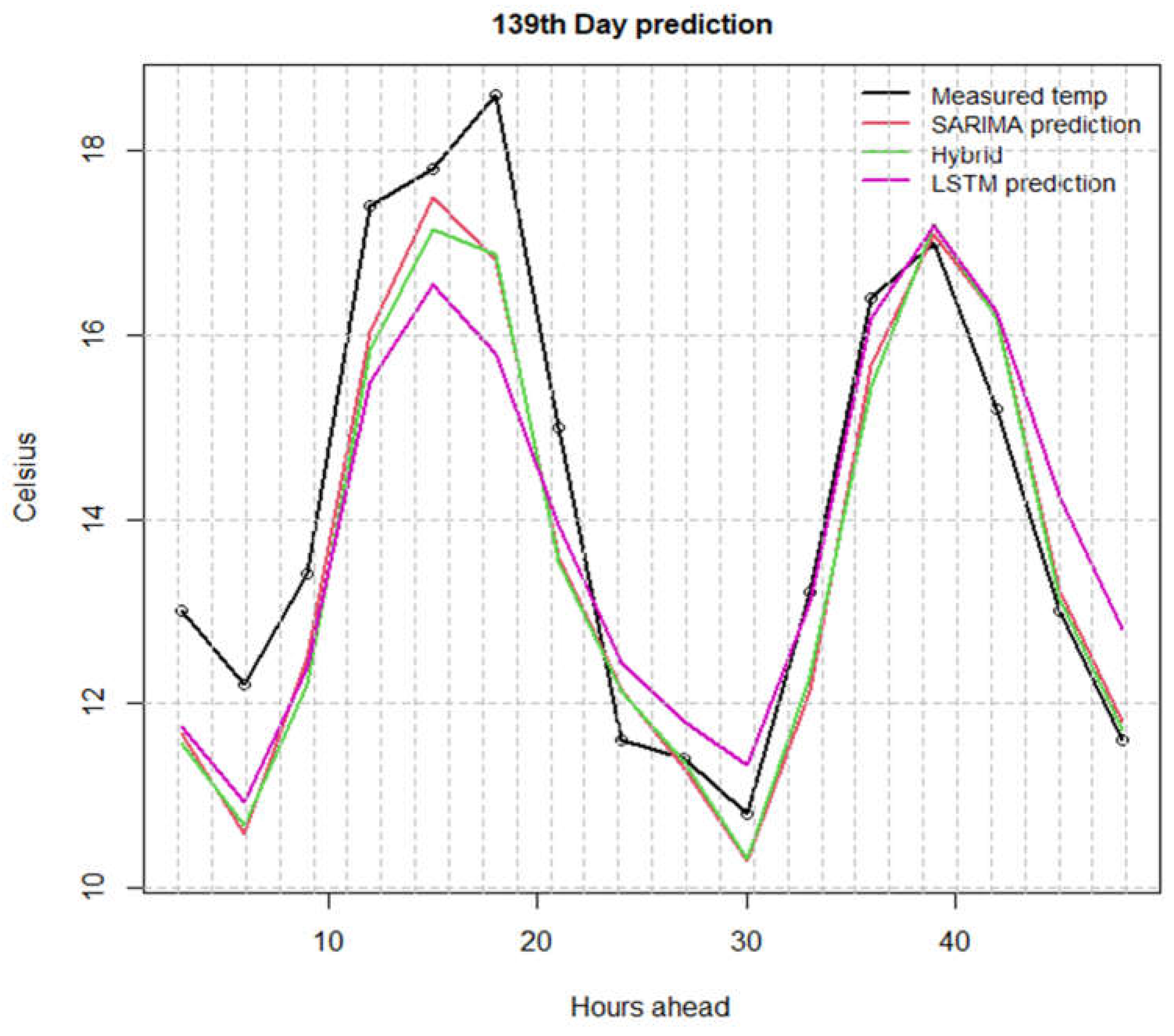
By analysing specific dates of the dataset, we present the different behaviours of the three methods in different weather conditions. The days that are individually chosen to be shown in the next figures are selected based mainly on the daily MAE of Figure 3, which are indicated with small squares in that graph. It is either extreme cases of small/big MAE errors, or instances where the preferred method is not what would be expected from the average values shown in Table 1. Additionally, we calculate the daily MAE of these days and comment on it under the scope of the temperature range, since it might be more important for a predictor to be able to forecast warmer/colder days with more/less temperature range.
The goal here is to examine when the methods fail and it would be extremely useful to determine if there is a causal effect that links the weather conditions with the best predictor. Then, one could inform a posteriori, depending on the meteorological conditions of the present or previous days on which method could predict the future more accurately, and thus construct another hybrid technique that would by definition lower the average MAE by choosing the method of least MAE for every day’s forecast.
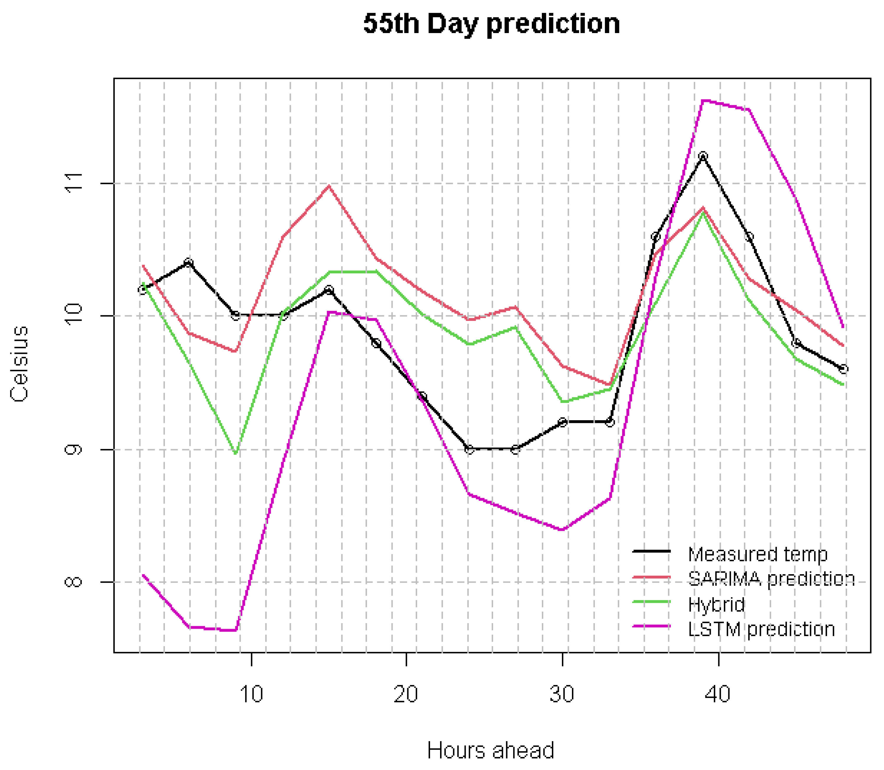
In Figure 4 we present an example of a prediction day from the test set, which is in January, characterized by a low temperature of 9 degrees at night, and a low range that reaches 11.2 degrees during the day. This is not unusual during the winter months, and we see great agreement between all methods. For that example of a 2-day prediction horizon, the calculated MAEs are: LSTM = 0.87, SARIMA = 0.48 and hybrid = 0.43, which is consistent with our average results that indicate the hybrid has a better fit in the test dataset overall. Nevertheless, we see in Figure 4 that the highest values of the second day are very well approximated by both the SARIMA and the hybrid, with the hybrid being a correction to the SARIMA during the first day, and an underprediction during the higher values of the second day. Other days the correction of the hybrid is not so pronounced, but on average, as Table 1 suggests, it is a useful improvement over the standard SARIMA model. Another meaningful observation of Figure 4 is that the LSTM might have severely underpredicted the low of the first day but reached the higher values that occurred during noon (at 12 and 39 h ahead in Figure 4). It is worth commenting that this example does not have the typical parabolic shape that daily temperature profiles usually exhibit, and that the small range plays a big role in the low MAE that is found. As we see in Figure 2 and Figure 3, in the summer months when the daily range is much higher and the maximum daily temperatures can exceed 40 degrees, the average MAE increases, especially with the LSTM method.
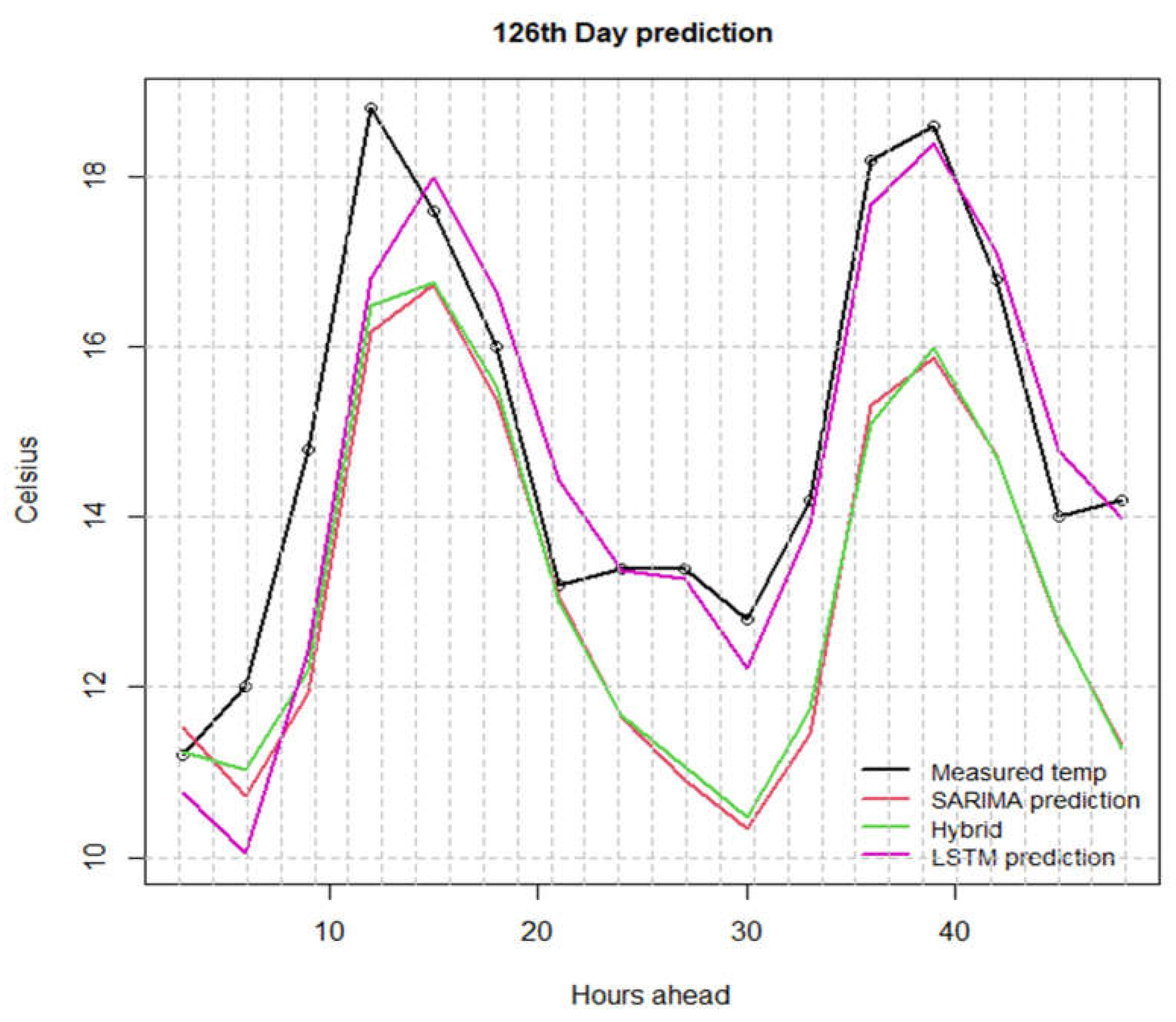
An example during March is presented in Figure 5. In this example it is shown that an LSTM method has a very good agreement, which is the inverse result of the averaged outcome of Table 1. In Figure 5 it is presented that the MAEs in that day for LSTM, SARIMA and hybrid were 0.75, 1.87 and 1.76, respectively. The range here is normal, from a low of 11.3 to a high of 19 degrees, and the parabolic pattern of temperature is stable between the two days, with consistent extremes. Between the SARIMA and the hybrid, we see that the hybrid prediction increases the underpredicted values of the SARIMA by a small margin, which constitutes an improvement.
In Figure 6, which is during the same month as Figure 5, we observe again that when there is a stable temperature profile, all three methods give accurate results with a reported MAE of LSTM = 1.02, SARIMA = 0.82 and hybrid = 0.87. In this case, the LSTM is worse than the other two methods, but the reason this example is interesting is that the hybrid is not a correction of the SARIMA. Indeed, the most pronounced difference of the hybrid and SARIMA occurs during the first day peak, where the hybrid is below the line of the SARIMA, and this results in a higher MAE of the hybrid for this example.
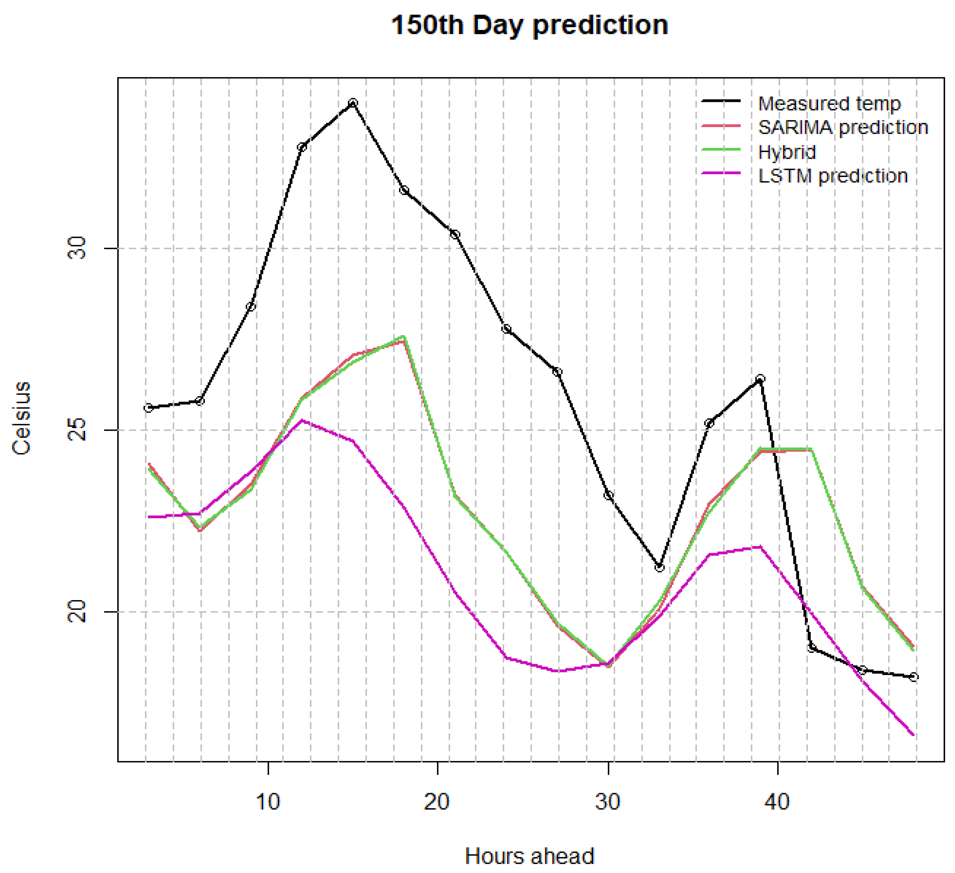
In Figure 7 we present a case during April (150th day mark of Figure 3), where the biggest MAEs are found. In this case, the highest value of 34.2 degrees followed by a low of 21 in the same day, and a low of 18 the next day renders all three methods unreliable for the specific example. The calculated MAE for the example is LSTM = 5.02, SARIMA = 4.19 and hybrid = 4.18, which does not represent an acceptable forecast.
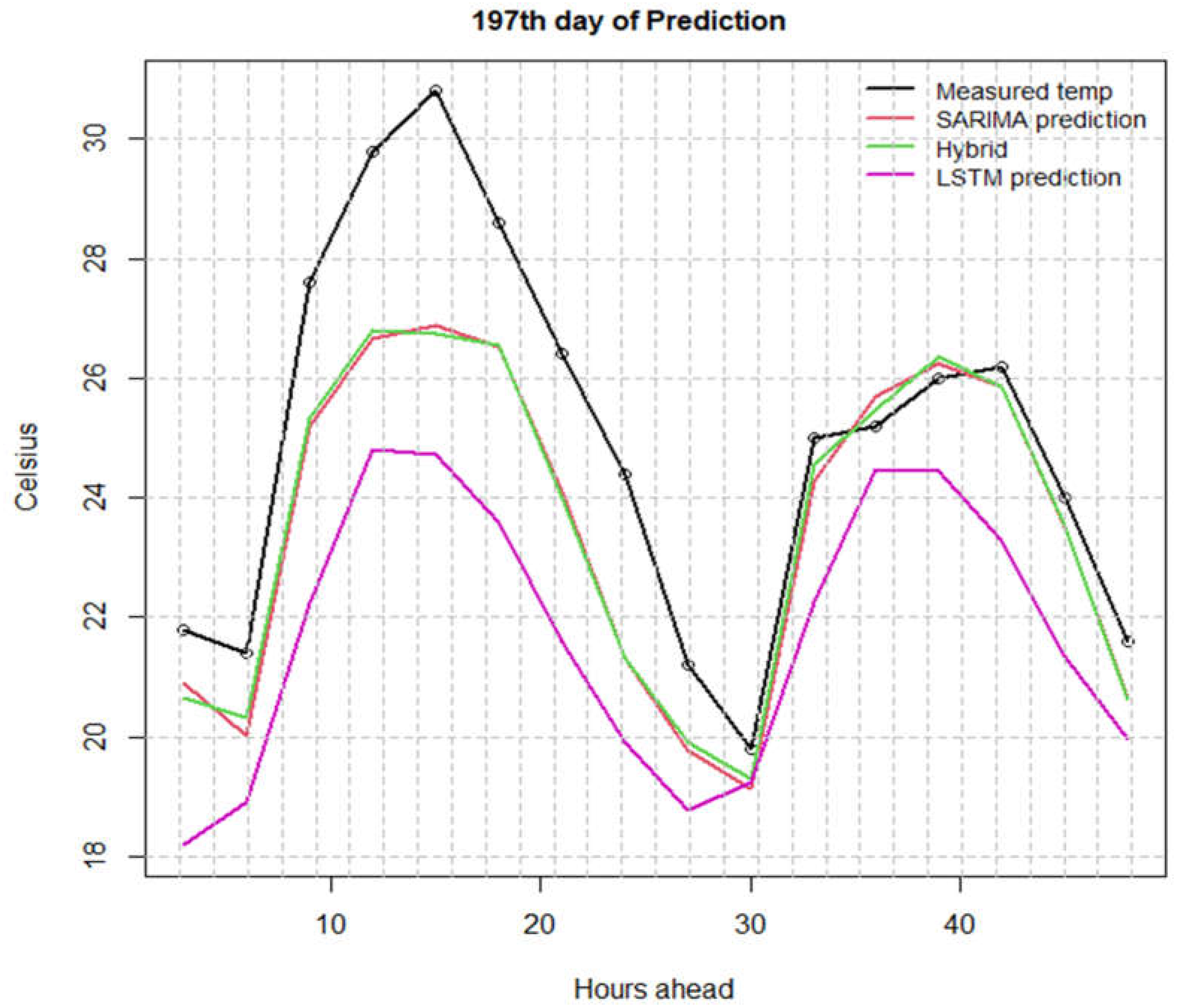
In Figure 8, a day in June is presented (fifth box in Figure 3), where the temperature range is also high, and the first day’s high is not well predicted, but the second day is very well predicted, especially by the SARIMA and the hybrid. More specifically, the 2-day MAE for Figure 8 are LSTM = 3.25, SARIMA = 1.53 and hybrid = 1.48. The hybrid increases accuracy upon the SARIMA, and the poor LSTM fit is also reflected by the MAE error which is more than double that of the hybrid MAE. This example is part of the higher temperature months where the 2-day temperature range can exceed 10 degrees Celsius and we often see an advantage of the SARIMA and the hybrid over the LSTM model.
In summary, in Figure 4, Figure 5, Figure 6, Figure 7 and Figure 8 we see that both the ARIMA and the LSTM can predict relatively well the temperature of the next two days, similar to the results of Table 1. The interesting outcome that is not reflected in the averaged values of Table 1 is that the question of the best method for each day does not have a clear answer, since for most days the SARIMA and hybrid are best suited, but on other days the LSTM has lower MAE. This result raises the question of the weather characteristics that may or may not affect the comparison between the predictors on different days. Our analysis and explanation of the individual results of Figure 4, Figure 5, Figure 6, Figure 7 and Figure 8 indicate that the range of the temperature might be a parameter that could inform such a decision, as the worst predictions occur not randomly, but at periods where big ranges exist, and huge shifts between 2–3 days can occur.
For the relative humidity, we see in Table 1 that the LSTM outperformed both methods, followed by the hybrid, which again corrected the SARIMA by a small margin. The fact that LSTM outperformed and decreased the margin in all examples in the 2-day forecast is consistent with the authors of [17] who note that the more days we try to forecast, the worse the SARIMA method performs and the better predictors are the deep neural networks. This affects the performance of the hybrid method, which is strongly related to the performance of the SARIMA.
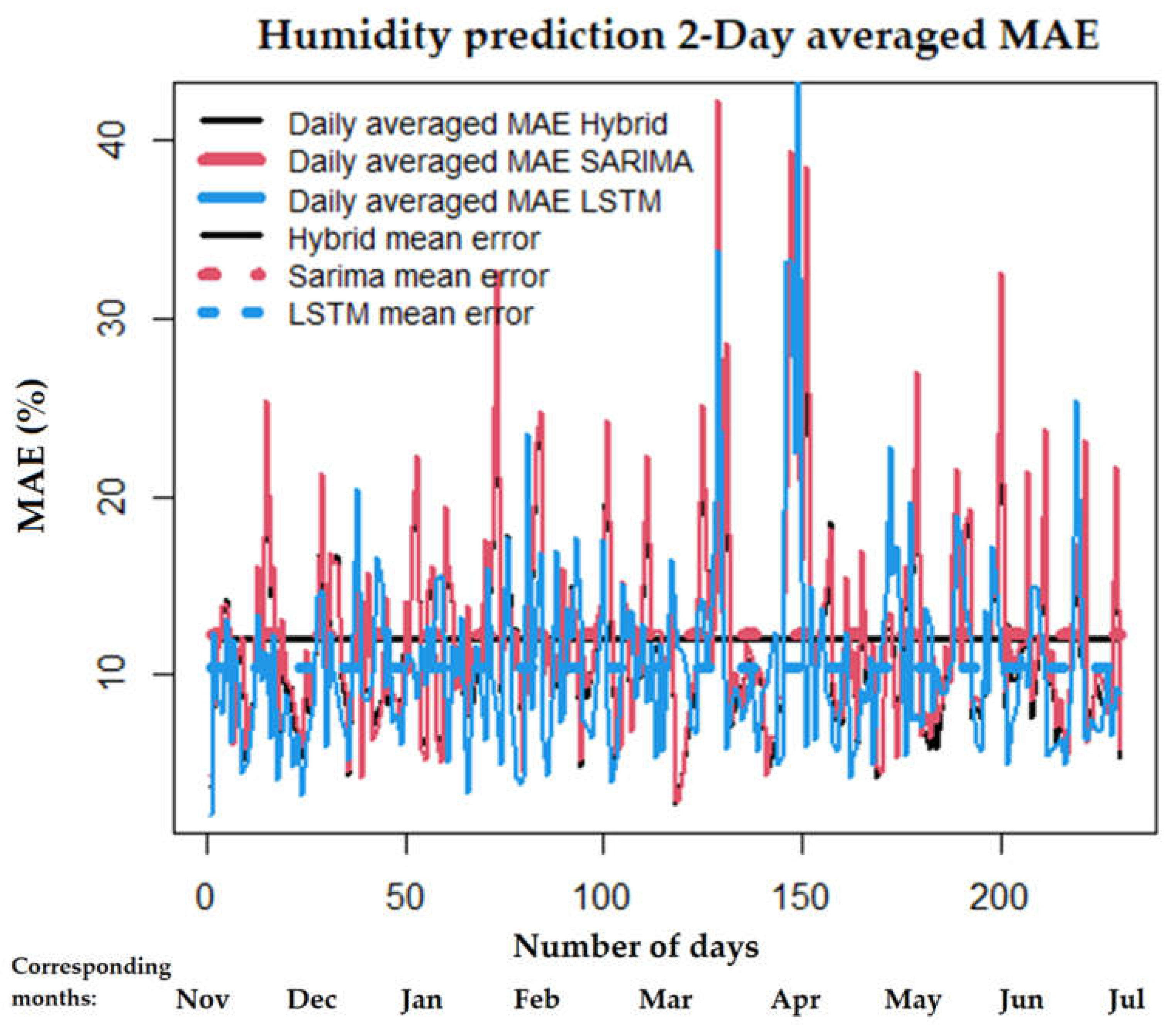
In Figure 9 we repeat the errors computed in Figure 3 for humidity, and we see in this case that there is a peak at the 150-day mark, similar to the temperature example, but the MAE after that threshold does not increase for the LSTM model, which keeps a more consistent error magnitude throughout.
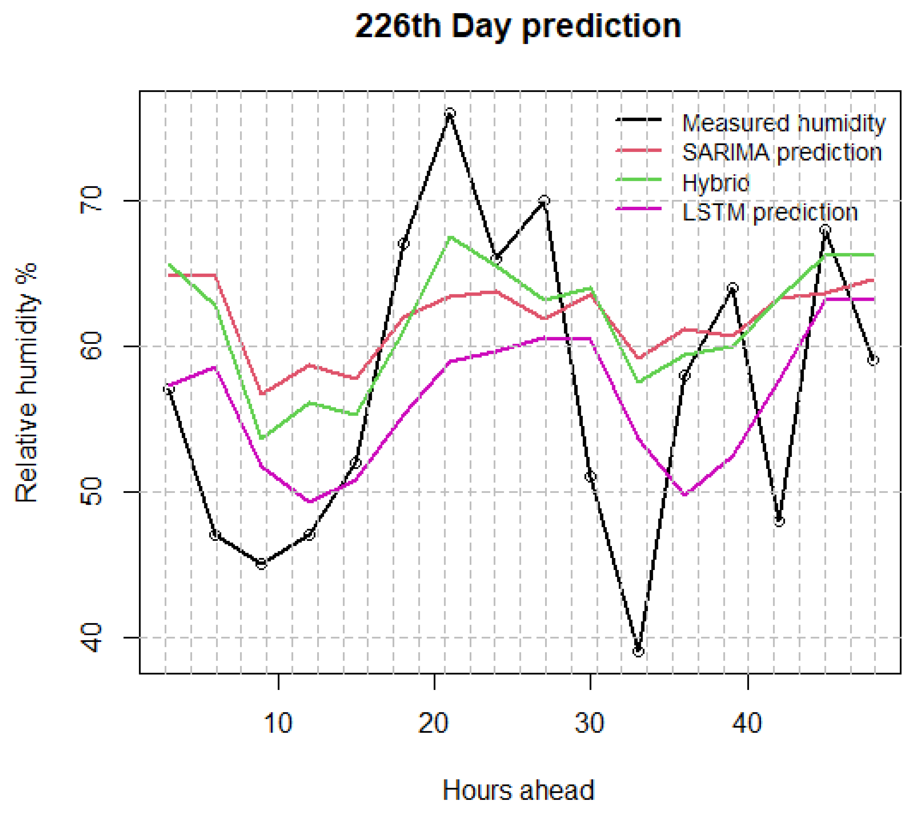
Finally, in Figure 10 we show an example in June with predictions that achieved an adequate performance from all three methods. Indeed, we calculate the 2-day MAE as LSTM = 8.09%, SARIMA = 9.19% and hybrid = 8.01% for that example.
Due to the similarity of the discussions and conclusions of humidity predictions with the temperature prediction in figure form, additional figures are omitted.

3.2. Wind Speed Forecast

Lastly, a presentation analogous to the previous section is being done here for the wind speed (m/s), which is considered the more chaotic variable of the three, with no obvious daily pattern like the temperature/humidity pair.
As we see in Table 1 in the wind speed section, the hybrid has the best average MAE among both SARIMA and the LSTM, but the correction of the hybrid over the SARIMA was by a small percentage of 3%. Additionally, the 2-day forecast showed a very small margin between the errors compared to the 1-day forecast horizon.
Similar to before, we see in Figure 11 the daily averaged MAE for the 2-day wind prediction of the first 230 days in the test set. Unlike before, we do not see an increase at the 150th day mark and afterwards; the tail of the error plot is significantly smaller than the first part. This can be related to the higher wind speeds and weather changes which are more prominent in the first part compared to the latter.
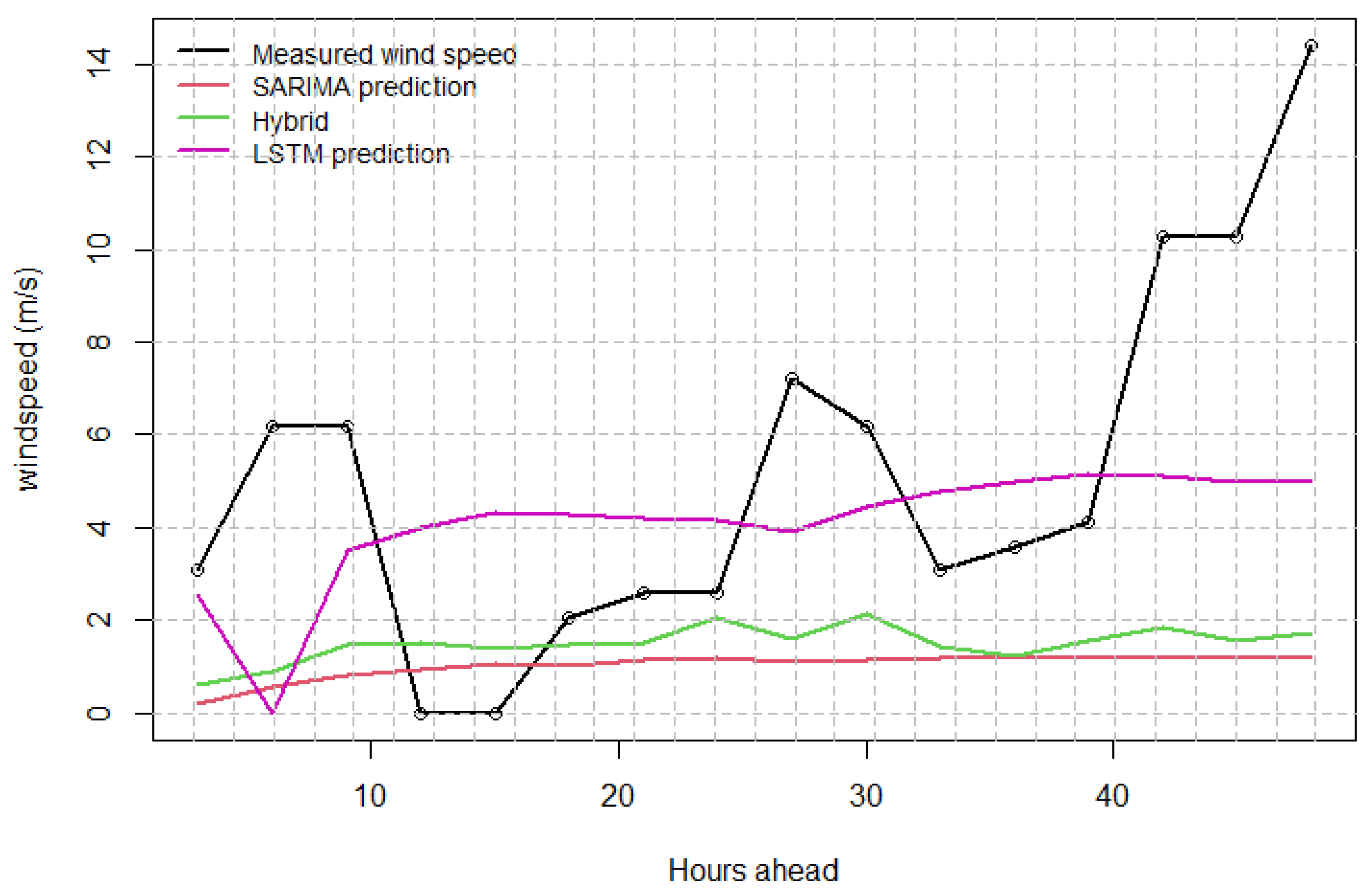
Additionally, we see in Figure 12 that all methods have difficulty in capturing the zero speed wind that is a possibility in wind prediction, and they also fail to predict the increase in the second day wind speeds as an extreme phenomenon, but the methods provide an estimate on the next 2 days’ wind, with a clear advantage on the LSTM. Indeed, we calculate the 2-day MAE of Figure 12 to be LSTM = 2.18, SARIMA = 4.34 and hybrid = 3.97. The hybrid is a correction over the SARIMA in this case, although it is not better than the LSTM, since the hybrid is heavily reliant on the SARIMA prediction. Lastly, we note that the case of Figure 12 is an example where low wind speeds have been reported during the previous days, which explains why the SARIMA and hybrid are extremely low and the LSTM has a zero prediction at 6 h ahead, although it is significantly better at predicting the rest of the hours.
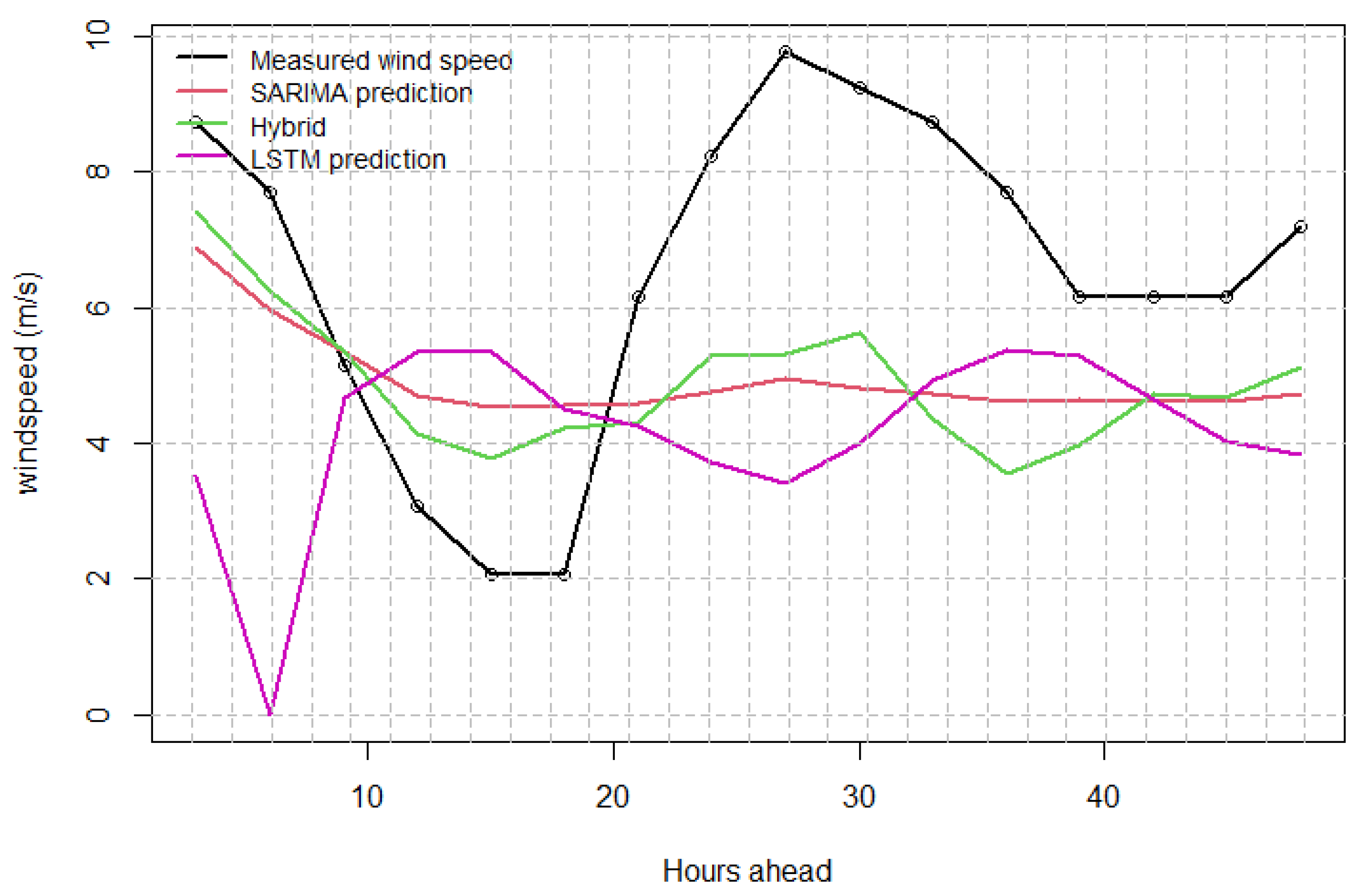
Another case of 2-day wind speed forecasting is presented in Figure 13 where the wind speed that was recorded during the previous hours had a big magnitude of approximately 10 m/s. In this case, we find the best method to be the hybrid by comparing their MAE, which are LSTM = 2.81, SARIMA = 2.43 and hybrid = 2.28. We also note that the SARIMA tends to predict around the mean value of the measured wind speed, whereas the hybrid tends to predict very well the added residual to the SARIMA. Judging by Figure 12 and Figure 13, a different best method outcome can be made for each. This adds to the ambiguity on the choice of the better method, and points towards the need for more research and deeper understanding of such methods, and the inherent chaotic nature that the wind speed time series exhibits.

4. Discussion—Future Work

In this work we introduced the hybrid method and we compared its results with the SARIMA and the LSTM NN on three meteorological variables for a time horizon of 1 and 2 days ahead. The hybrid was shown to be better overall at the examples of temperature and wind speed prediction, whereas the LSTM compared well and was even preferred on the average errors of relative humidity prediction.
The results indicate that in cases of extreme weather conditions and when the weather changes abruptly, the predictions are heavily unreliable. This is the biggest source of the errors that are emphasized by Figure 7, Figure 8 and Figure 13 and increased our averaged errors in Table 1. With that in mind, these situations can be considered as special cases and not the norm for the dataset under consideration as Figure 2, Figure 3, Figure 9 and Figure 11 indicate, where most of the days have low MAE and there are spikes of high error in some circumstances. Thus, the resulting errors in Table 1 (that include both the stable and the few extreme weather change incidents) are at an acceptable scale. This agrees well with the literature, see, e.g., [36], where data-driven models are proposed to forecast extreme events like floods. NN and LSTMs are being used to simulate the rainfall-runoff process using 15 rainfall and hydrologic stations collecting in situ data for nearly 40 years. Their outcome indicates that LSTM is the most appropriate form of NN for such applications, and that more data may be needed to increase the accuracy of the methods, which comes with an increase in money, resources and computations. The reduction of error can be achieved in other ways, which is the reason why we introduced our hybrid method that, in some cases, achieved up to 10% MAE reduction compared to the standard LSTM and SARIMA methods.
The computational cost added by the hybrid is not considered significant, and one can argue that this is “offline” computational cost, meaning that the training of the methods happens once, and then the model can predict each day without too much computational effort, so the computational time is an insignificant concern.
Our hybrid technique can be further improved by combining another back propagation network, so that instead of adding the SARIMA forecast and the residual forecast, one can search for the functional relationship between these two quantities. Similar work on a much less chaotic dataset is found in Deng at al. [29]. The LSTM and the SARIMA model performed comparably well and can both be utilized to predict the weather variables considered here adequately. Another hybrid approach with promising results that could be implemented for our problem is found in Dave at al. [41], where the time series is firstly decomposed into seasonal, trend and residual components, and then, different predictors are imposed on those different components. This could be combined with our hybrid approach or the previously mentioned one of Deng at al. [29]. In addition, a four-stage hybrid model for hydrological time series forecasting is introduced in Di at al. [19] with (i) denoising of the data, (ii) decomposition into multiple signals, (iii) prediction separately of the signals and (iv) ensemble using another neural network of all the decomposed prediction signals. Similar to other studies, the authors have multiple hydrological and meteorological stations, some working for over 60 years, which aids the accuracy of their results. Lastly, following [5] which focuses –on solar radiation prediction for a high density grid of meteorological stations, one could add different data sources and compare a model like the random forests that those authors implement with the methods we presented here. Since we are focused on a low-cost accurate prediction, the option of adding more stations to improve the datasets was not available and a fair comparison with such techniques in the literature is not possible.
One could argue that all this discussion about hybrid methodologies development and implementation is insignificant since the LSTM model we presented here as a base model is a very competitive option with the other models. We argue that the amount of work that it takes to optimize a LSTM model, fine tune the parameters, find the best working optimizers, activation functions, units for the layers, etc., becomes a significant downside for practical applications. Parameter tuning is necessary for the research setting and methodological comparison, but it is not ideal for real-world applications where multiple networks must be fitted for different locations, datasets and variables. Furthermore, the fact that it is not clear which days are predicted better with the LSTM and the SARIMA–hybrid combination is a clear indication that more research is needed towards developing more accurate methods.
Another way accuracy could be improved is by reframing the problem itself. To demonstrate, we will entertain an approach that will be implemented and tested in the future, and would eliminate the daily cyclic behaviour of temperature, which, as our tests have shown us, is an additional characteristic to predict and eliminating it could positively affect the prediction performance. This method can be applied to variables with periodic characteristics and simplify the datasets beforehand. By applying daily max–min–mean functions to our data, instead of predicting eight 3-h intervals for 1-day ahead, one could focus on predicting just one value using the daily averaged time series of maximum daily temperature, and analogously, train a different NN or SARIMA model on the minimum daily temperature time series. Having a prediction of the maximum and minimum temperature of the next day is of great importance. Furthermore, we can extend this to 3-h interval predictions by invoking interpolating polynomials, since the general pattern of the temperature variation is known, within certain tolerances. This methodology can be applied also to humidity and any other periodic variable, utilizing the usual parabolic shape of most days. On the downside, it might impose additional errors due to the interpolation of the polynomial, but it is expected to have better accuracy on the predictor side since the dataset is less noisy and smaller and thus easier to handle computationally. Additionally, the amount of prediction time steps decreases significantly to one (or two for the 2-day forecast). In our future work, it remains to be seen if this method or the other hybrid methods mentioned here provide improvements in the accuracy of the predictions.

5. Conclusions

Three prediction methods were implemented and compared for predicting weather variables, namely the SARIMA, the LSTM and our introduced hybrid methodology. SARIMA and LSTM were shown to perform adequately well for 1–2 day prediction horizons, by using localised time series. The results show that the examined hybrid methodology described here performs better at predicting the temperature and wind speed, closely followed by the SARIMA, whereas LSTM performs better overall at the humidity forecast, even after the correction of the hybrid to the SARIMA model. Several prediction examples from the test set were presented with the goal of examining various cases where the methods failed, since it would be useful to determine if there is a causal effect that links the weather conditions with the best predictor. The improvement of the hybrid was not so pronounced, especially considering the added computational cost and complexity (approximately 2 h of computing). On the other hand, the LSTM with two hidden layers and a significant amount of parameter fine tuning, was usually outperformed by the other methods, especially in the 1-day forecasts, but in the 2-day forecasts it closed the gap. The future challenge is to further increase accuracy, and as proposed in the discussion section, use a combination of these techniques, apply new hybrid techniques or even reframe the problem in order to achieve it. Finally, the methods would preferably require minimal expert knowledge, testing time from scientific personnel and cost of computing capabilities so that these methods can be utilized in an operational forecasting setting and have a wider range of applications in everyday life.

Author Contributions

Conceptualization, A.P. and G.A.; methodology, A.P.; software, A.P.; validation, A.P.; formal analysis, A.P. and G.A.; investigation, A.P., G.A., K.S., G.V.K. and N.A.K.; resources, A.P., K.S., G.V.K. and N.A.K.; data curation, A.P., K.S., G.V.K. and N.A.K.; writing—original draft preparation, A.P. and G.A.; writing—review and editing, A.P., G.A., K.S., G.V.K. and N.A.K.; visualization, A.P.; supervision, G.A. and N.A.K.; project administration, G.A. and N.A.K.; funding acquisition, G.A. and N.A.K. All authors have read and agreed to the published version of the manuscript.

Funding

This work was financially supported by the project “Meteorological, Bioclimatic and oceanographic information display system for tourist applications (SmarTourism)” under the code MIS 5029194 under the RIS3Crete co-funded by Greece and European Union.

Institutional Review Board Statement

Not applicable.

Informed Consent Statement

Not applicable.

Data Availability Statement

Additional data to our MS were provided by the Hellenic National Meteorological Service and can be downloaded freely from (http://www.emy.gr/emy/el/services/paroxi-ipiresion-elefthera-dedomena accessed on 9 December 2021). Our MS data are available upon request.

Acknowledgments

The authors would like to thank the two unknown reviewers for their comments and suggestions that were crucial in the final shaping of this work.

Conflicts of Interest

The authors declare no conflict of interest.

References

  1. Bochenek, B.; Ustrnul, Z. Machine Learning in Weather Prediction and Climate Analyses—Applications and Perspectives. Atmosphere 2022, 13, 180. [Google Scholar] [CrossRef]
  2. Georgopoulou, E.; Mirasgedis, S.; Sarafidis, Y.; Hontou, V.; Gakis, N.; Lalas, D.P. Climatic preferences for beach tourism: An empirical study on Greek islands. Theor. Appl. Climatol. 2019, 137, 667–691. [Google Scholar] [CrossRef]
  3. Elmira, J.; Remaz, O.D. Intra Urban Air Temperature Distributions in Historic Urban Center. Am. J. Environ. Sci. 2012, 8, 503. [Google Scholar]
  4. Scott, D.; Lemieux, C. Weather and Climate Information for Tourism. Procedia Environ. Sci. 2010, 1, 146–183. [Google Scholar] [CrossRef] [Green Version]
  5. Zeng, Z.; Wang, Z.; Gui, K.; Yan, X.; Gao, M.; Luo, M.; Geng, H.; Liao, T.; Li, X.; An, J.; et al. Daily Global Solar Radiation in China Estimated From High-Density Meteorological Observations: A Random Forest Model Framework. Earth Space Sci. 2020, 7, e2019EA001058. [Google Scholar] [CrossRef] [Green Version]
  6. Shih, H.; Rajendran, S. Comparison of Time Series Methods and Machine Learning Algorithms for Forecasting Taiwan Blood Services Foundation’s Blood Supply. J. Health Eng. 2019, 2019, 6123745. [Google Scholar] [CrossRef]
  7. Sillmann, J.; Thorarinsdottir, T.; Keenlyside, N.; Schaller, N.; Alexander, L.V.; Hegerl, G.; Seneviratne, S.I.; Vautard, R.; Zhang, X.; Zwiers, F.W.; et al. Understanding, modeling and predicting weather and climate extremes: Challenges and opportunities. Weather. Clim. Extrem. 2017, 18, 65–74. [Google Scholar] [CrossRef]
  8. Wilks, D.S.; Wilby, R.L. The weather generation game: A review of stochastic weather models. Prog. Phys. Geogr. Earth Environ. 1999, 23, 329–357. [Google Scholar] [CrossRef]
  9. Shankarnarayan, V.K.; Ramakrishna, H. Comparative study of three stochastic future weather forecast approaches: A case study. Data Sci. Manag. 2021, 3, 3–12. [Google Scholar] [CrossRef]
  10. Box, G. Box and Jenkins: Time Series Analysis, Forecasting and Control. In A Very British Affair: Six Britons and the Development of Time Series Analysis during the 20th Century; Mills, T.C., Ed.; Palgrave Macmillan UK: London, UK, 2013; pp. 161–215. [Google Scholar]
  11. Hyndman, R.J.; Athanasopoulos, G. Forecasting: Principles and Practice; OTexts: Melbourne, Australia, 2014. [Google Scholar]
  12. Grigonytė, E.; Butkevičiūtė, E. Short-term wind speed forecasting using ARIMA model. Energetika 2016, 62, 1–2. [Google Scholar] [CrossRef] [Green Version]
  13. Lai, Y.; Dzombak, D.A. Use of the Autoregressive Integrated Moving Average (ARIMA) Model to Forecast Near-Term Regional Temperature and Precipitation. Weather Forecast. 2020, 35, 959–976. [Google Scholar] [CrossRef]
  14. Jayawardena, A.; Gurung, A. Noise reduction and prediction of hydrometeorological time series: Dynamical systems approach vs. stochastic approach. J. Hydrol. 2000, 228, 242–264. [Google Scholar] [CrossRef]
  15. Paulescu, M.; Paulescu, E.; Gravila, P.; Badescu, V. Time Series Forecasting. In Weather Modeling and Forecasting of PV Systems Operation; Paulescu, M., Paulescu, E., Gravila, P., Badescu, V., Eds.; Springer: London, UK, 2013. [Google Scholar]
  16. Tylkowski, J.; Hojan, M. Time Decomposition and Short-Term Forecasting of Hydrometeorological Conditions in the South Baltic Coastal Zone of Poland. Geosciences 2019, 9, 68. [Google Scholar] [CrossRef] [Green Version]
  17. Kreuzer, D.; Munz, M.; Schlüter, S. Short-term temperature forecasts using a convolutional neural network—An application to different weather stations in Germany. Mach. Learn. Appl. 2020, 2, 100007. [Google Scholar] [CrossRef]
  18. Kuhn, M.; Johnson, K. Applied Predictive Modeling, 1st ed.; Springer Science Business Media: New York, NY, USA, 2018; p. 600. [Google Scholar]
  19. Di, C.; Yang, X.; Wang, X. A Four-Stage Hybrid Model for Hydrological Time Series Forecasting. PLoS ONE 2014, 9, e104663. [Google Scholar] [CrossRef]
  20. Jain, A.; Kumar, A.M. Hybrid neural network models for hydrologic time series forecasting. Appl. Soft Comput. 2007, 7, 585–592. [Google Scholar] [CrossRef]
  21. Wang, W.; Van Gelder, P.H.; Vrijling, J.; Ma, J. Forecasting daily streamflow using hybrid ANN models. J. Hydrol. 2006, 324, 383–399. [Google Scholar] [CrossRef]
  22. Chen, P.; Niu, A.; Liu, D.; Jiang, W.; Ma, B. Time Series Forecasting of Temperatures using SARIMA: An Example from Nanjing. IOP Conf. Ser. Mater. Sci. Eng. 2018, 394, 052024. [Google Scholar] [CrossRef]
  23. Ray, S.; Das, S.S.; Mishra, P.; Al Khatib, A.M.G. Time Series SARIMA Modelling and Forecasting of Monthly Rainfall and Temperature in the South Asian Countries. Earth Syst. Environ. 2021, 5, 531–546. [Google Scholar] [CrossRef]
  24. Dwivedi, D.K.; Kelaiya, J.; Sharma, G.R. Forecasting monthly rainfall using autoregressive integrated moving average model (ARIMA) and artificial neural network (ANN) model: A case study of Junagadh, Gujarat, India. J. Appl. Nat. Sci. 2019, 11, 35–41. [Google Scholar] [CrossRef]
  25. Zhang, G.P. Time series forecasting using a hybrid ARIMA and neural network model. Neurocomputing 2003, 50, 159–175. [Google Scholar] [CrossRef]
  26. Tealab, A. Time series forecasting using artificial neural networks methodologies: A systematic review. Future Comput. Inform. J. 2018, 3, 334–340. [Google Scholar] [CrossRef]
  27. Hajirahimi, Z.; Khashei, M. Hybrid structures in time series modeling and forecasting: A review. Eng. Appl. Artif. Intell. 2019, 86, 83–106. [Google Scholar] [CrossRef]
  28. Saba, T.; Rehman, A.; AlGhamdi, J.S. Weather forecasting based on hybrid neural model. Appl. Water Sci. 2017, 7, 3869–3874. [Google Scholar] [CrossRef] [Green Version]
  29. Deng, Y.; Fan, H.; Wu, S. A hybrid ARIMA-LSTM model optimized by BP in the forecast of outpatient visits. J. Ambient Intell. Humaniz. Comput. 2020, 1–11. [Google Scholar] [CrossRef]
  30. Mieczkowski, Z. The tourism climatic index: A method of evaluating world climates for tourism. Can. Geogr. Le Géographe Can. 1985, 29, 220–233. [Google Scholar] [CrossRef]
  31. Rutty, M.; Scott, D.; Matthews, L.; Burrowes, R.; Trotman, A.; Mahon, R.; Charles, A. An Inter-Comparison of the Holiday Climate Index (HCI:Beach) and the Tourism Climate Index (TCI) to Explain Canadian Tourism Arrivals to the Caribbean. Atmosphere 2020, 11, 412. [Google Scholar] [CrossRef] [Green Version]
  32. Hyndman, R.J.; Khandakar, Y. Automatic Time Series Forecasting: The forecast Package for R. J. Stat. Softw. 2008, 27, 1–22. [Google Scholar] [CrossRef] [Green Version]
  33. Hyndman, R.J.; Athanasopoulos, G.; Bergmeir, C.; Caceres, G.; Chhay, L.; O’Hara-Wild, M.; Petropoulos, F.; Razbash, S.; Wang, E.; Yasmeen, F.; et al. Forecast: Forecasting Functions for Time Series and Linear Models. 2021. Available online: https://cran.r-project.org/web/packages/forecast/forecast.pdf (accessed on 20 May 2022).
  34. Petnehazi, G. Recurrent Neural Networks for Time Series Forecasting. arXiv 2018, arXiv:1901.00069. [Google Scholar]
  35. Lewis, N.D.C. Neural Networks for Time Series Forecasting with R: An Intuitive Step by Step Blueprint for Beginners; AusCov: Scotts Valley, CA, USA, 2017. [Google Scholar]
  36. Hu, C.; Wu, Q.; Li, H.; Jian, S.; Li, N.; Lou, Z. Deep Learning with a Long Short-Term Memory Networks Approach for Rainfall-Runoff Simulation. Water 2018, 10, 1543. [Google Scholar] [CrossRef] [Green Version]
  37. Elsaraiti, M.; Merabet, A. A Comparative Analysis of the ARIMA and LSTM Predictive Models and Their Effectiveness for Predicting Wind Speed. Energies 2021, 14, 6782. [Google Scholar] [CrossRef]
  38. Ruder, S. An Overview of Gradient Descent Optimization Algorithms. arXiv 2016, arXiv:1609.04747, 4747. [Google Scholar]
  39. Kingma, D.P.; Ba, J. Adam: A Method for Stochastic Optimization. arXiv 2015, arXiv:1412.6980. [Google Scholar]
  40. Pappenberger, F.; Ramos, M.H.; Cloke, H.L.; Wetterhall, F.; Alfieri, L.; Bogner, K.; Mueller, A.; Salamon, P. How do I know if my forecasts are better? Using benchmarks in hydrological ensemble prediction. J. Hydrol. 2015, 522, 697–713. [Google Scholar] [CrossRef] [Green Version]
  41. Dave, E.; Leonardo, A.; Jeanice, M.; Hanafiah, N. Forecasting Indonesia Exports using a Hybrid Model ARIMA-LSTM. Procedia Comput. Sci. 2021, 179, 480–487. [Google Scholar] [CrossRef]
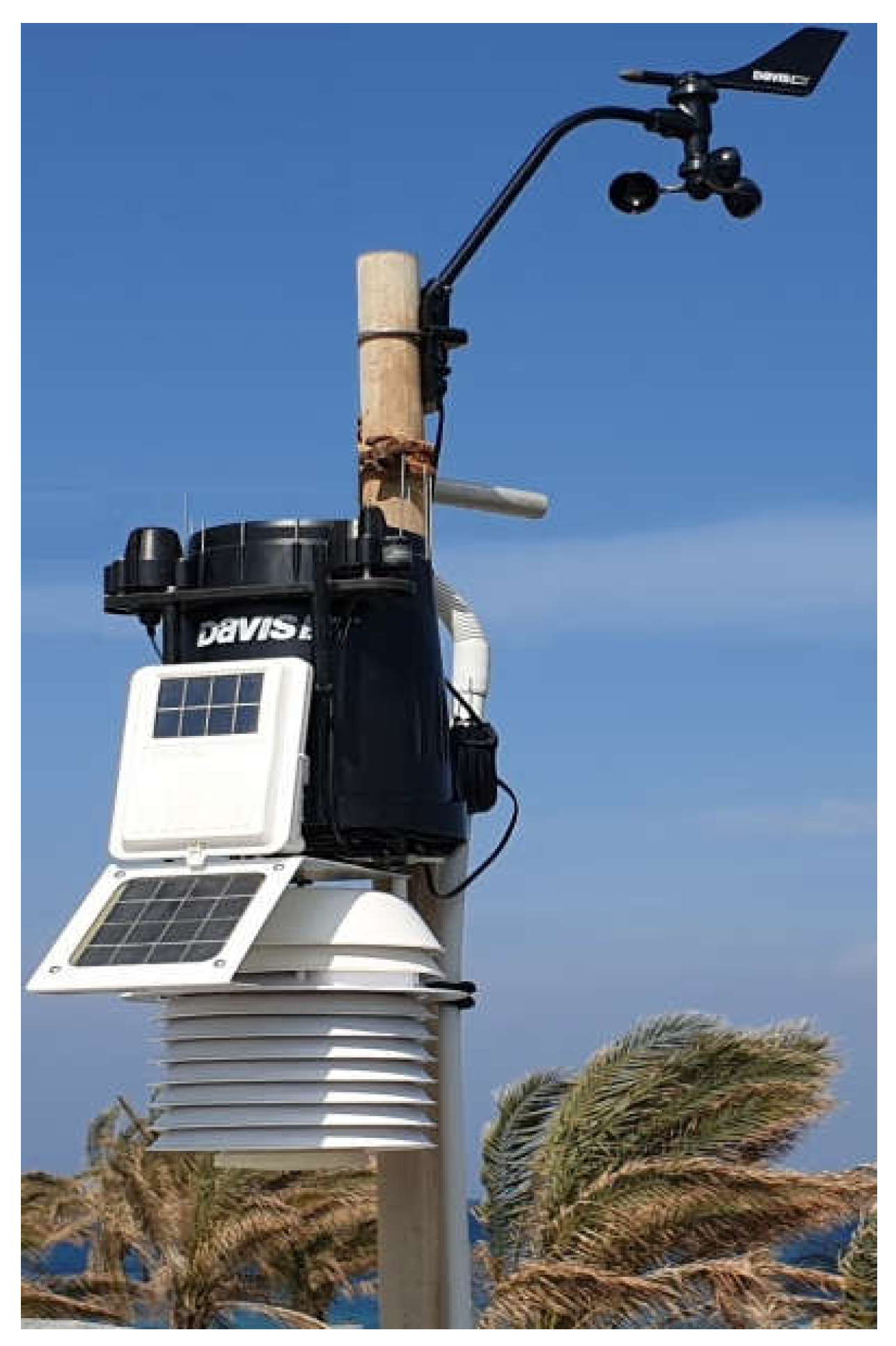
Figure 1. The meteorological station installed on a hotel rooftop in Crete, Greece.
Atmosphere 13 00878 g001
Figure 2. Comparison of SARIMA, LSTM and hybrid using daily averaged MAE with real data for 1-day prediction horizon for 230 days of the test set. With dashed lines the average error of all the dataset is shown. Units of MAE are in Celsius in this temperature example.
Atmosphere 13 00878 g002
Figure 3. Comparison of SARIMA, LSTM and hybrid using daily averaged MAE with real data for 2-day prediction horizon for 230 days of the test set. With dashed lines the average error of all the dataset is shown. The boxes indicate the predictions that we plot separately to observe their 48-h behaviour. Units of MAE are in Celsius in this temperature example.
Atmosphere 13 00878 g003
Figure 4. Comparison of SARIMA, LSTM and hybrid with real data on temperature example for 2-day prediction horizon in January.
Atmosphere 13 00878 g004
Figure 5. Comparison of SARIMA, LSTM and hybrid with real data on temperature example for 2-day prediction horizon during March; stable parabolic temperature profile.
Atmosphere 13 00878 g005
Figure 6. Comparison of SARIMA, LSTM and hybrid with real data on temperature example for 2-day prediction horizon in March; stable temperature example where hybrid is not achieving a correction on the SARIMA.
Atmosphere 13 00878 g006
Figure 7. Comparison of SARIMA, LSTM and hybrid with real data on temperature example for 2-day prediction horizon in April; example with very big MAE.
Atmosphere 13 00878 g007
Figure 8. Comparison of SARIMA, LSTM and hybrid with real data on temperature example for 2-day prediction horizon in June; example with very big MAE.
Atmosphere 13 00878 g008
Figure 9. Comparison of SARIMA, LSTM and hybrid using daily averaged MAE with real data for 2-day prediction horizon on humidity prediction for 230 days of the test set. With dashed lines the average error of all the dataset is shown. Units of MAE are in percentage (%) in this humidity example.
Atmosphere 13 00878 g009
Figure 10. Comparison of SARIMA, LSTM and hybrid with real data on humidity example for 2-day prediction horizon in June; example with very big MAE.
Atmosphere 13 00878 g010
Figure 11. Comparison of SARIMA, LSTM and hybrid using daily averaged MAE with real data for 2-day prediction horizon on wind speed prediction for 230 days of the test set. With dashed lines the average error of all the dataset is shown. Units of MAE are in m/s in this wind speed example.
Atmosphere 13 00878 g011
Figure 12. Comparison of SARIMA, LSTM and hybrid with real data for 2-day prediction horizon during December; wind speed example; low wind speed during previous days.
Atmosphere 13 00878 g012
Figure 13. Comparison of SARIMA, LSTM and hybrid with real data for 2-day prediction horizon during May; wind speed example; high wind speed during previous days.
Atmosphere 13 00878 g013
Table 1. MAE errors for the three methods for 1- and 2-day prediction of wind speed (m/s) for the three predicted variables, averaged over each day and then over the test set. MAE units are the same as the predicted variable.
Prediction VariableMethodsMAE 1-DayMAE 2-Day
Temperature (Celsius)SARIMA (1, 0, 2) (2, 1, 2)1.581.86
LSTM
(Adam 40 units each of two hidden layers)
2.122.14
Hybrid1.561.85
Climatological benchmark2.252.26
Persistence benchmark2.442.44
Humidity (%)SARIMA (5, 1, 0) (2, 0, 0)10.62%12.33%
LSTM
(Adam 40 units each of two hidden layers)
9.54%10.01%
Hybrid10.30%12.01%
Climatological benchmark11.15%11.16%
Persistence benchmark14.14%14.16%
Wind Speed (m/s)SARIMA (0, 1, 5) (0, 0, 2)2.462.78
LSTM
(Adam 60 units each of two hidden layers)
2.732.79
Hybrid2.412.70
Climatological benchmark2.872.88
Persistence benchmark3.673.68
Publisher’s Note: MDPI stays neutral with regard to jurisdictional claims in published maps and institutional affiliations.