Abstract
As the world is moving toward greener forms of energy, to mitigate the effects of global warming due to greenhouse gas emissions, wind energy has risen as the most invested-in renewable energy. China, as the largest consumer of world energy, has started investing heavily in wind energy resources. Most of the wind farms in China are located in Northern China, and they possess the disadvantage of being far away from the energy load. To mitigate this, recently, offshore wind farms are being proposed and invested in. As an initial step in the wind farm setting, a thorough knowledge of the wind energy potential of the candidate region is required. Here, we conduct numerical experiments with Weather Research and Forecasting (WRF) model forced by analysis (NCEP-FNL) and reanalysis (ERA-Interim and NCEP-CFSv2) to find the best choice in terms of initial and boundary data for downscale in the South China Sea. The simulations are validated by observation and several analyses. Specific locations along China’s coast are analyzed and validated for their wind speed, surface temperature, and energy production. The analysis shows that the model forced with ERA-Interim data provides the best simulation of surface wind speed characteristics in the South China Sea, yet the other models are not too far behind. Moreover, the analysis indicates that the Taiwan Strait along the coastal regions of China is an excellent region to set up wind farms due to possessing the highest wind speeds along the coast.
1. Introduction
The development of any nation in our world is dependent on the energy it consumes. As the world is industrializing more, the world’s energy requirement has been increasing significantly in recent decades. To meet the energy demands, global nations have been using thermal power stations based on fossil fuels, nuclear power, and hydroelectric power. The world energy production in the year 2019 was about 31% from oil, 26% from coal, 23% from natural gas, 10% from electric power, 10% from biomass, and the rest from other sources [1]. Of this world production, 24.5% of global energy is consumed by China, 16.1% by the USA, with India coming third at 6% [1]. The countries, which were mainly dependent on fossil fuels for their energy sources, have been asked to reduce their emissions and their contributions to the global climate crisis in the last decade. In 2019, China’s dependence on nonrenewable energy sources is about 73% and it is trying to shift most of its energy production to renewable energy from wind and solar radiation. On the renewable energy front, the majority of the energy comes from hydroelectric followed by wind energy. Preliminary analysis of the first half of 2020 has shown that China’s energy production from renewable has increased up to 40% [2]. Even though hydroelectric is renewable, its environmental impact and feasibility have made wind energy the most investable source of future renewable energy investment. China has more than doubled its construction of wind and solar power plants in the year 2020 [2].
China’s wind energy farming is mainly focused on wind resources in the mountainous Northern China where the power load is minimum. Meanwhile, most of China’s power grids are located in Southeastern China along the coastal region [3,4]. Hence, most of the onshore wind energy potential of China is underutilized, as they are expensive to connect to the grid. Recently, there has been an incentive to increase the power production along the offshore region where the population and demand coexist. Offshore wind energy farms can be set up in the coastal region where the average depth of the ocean is less than 50 m. Eastern and Southeastern China have a coastal region that satisfies these criteria [5].
Wind energy production along the South China Sea has a significant seasonal variability, with most of the wind energy in the fall and winter seasons [6,7,8]. To maximize energy production, it is necessary to have a thorough understanding of the energy available for higher spatial–temporal resolution along the coastal regions of southern China. Data sources from satellites, in situ observations, and numerical weather forecast models pave our initial mode of analysis. Previous studies found that the South China Sea has been identified as having an excellent wind energy source. Figure 1 shows the terrain and bathymetry of the South China Sea and the surrounding region. Along the southern coast of China (Figure 1b), the continental shelf extends up to 100 km away from the coastal region with vast shallow coasts. With the lack of in situ data for offshore conditions, satellite data are used for wind energy analysis along the South China Sea [9,10,11,12]. With the onset of satellite data, Taiwan Strait along the South China Sea has been found to have the highest wind speed in the winter season (above 600 Wm−2) [13,14]. Satellite records steady wind speed during the fall and winter seasons (above 6 m s−1) in the central and northern parts of the South China Sea [15]. The satellite data is limited by temporal resolution, cloud cover, and constricted only to the surface. Data from global models, which have been accumulating for the past 25 years, can be used but they are not consistent or high resolution to analyze the recent variations [16]. Numerical weather prediction models are an excellent tool for analyzing the regional wind resources in a hindcast and forecast manner for understanding the resources at any location. Global wind atlases from numerical models are available which provides monthly climatology of wind speed across the globe at high resolutions, but they are not tailored for a particular region. In numerical weather prediction, the selection of initial and boundary conditions plays an important role in the model outcomes. These initial and boundary conditions are obtained mostly from global models which are run at a low resolution. Since there are many global models to obtain these data, we here analyze the performance of downscaling three widely used global reanalysis to simulate the wind conditions over the South China Sea and the surrounding region.
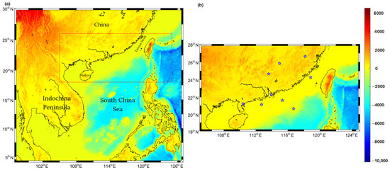
Figure 1.
(a) Terrain and Bathymetry (m) of South China Sea and surrounding region from ETOPO2 data. (b) Southern China coast showing the shallow bathymetry. The point locations used in the following analysis are shown as blue stars.
The numerical model, especially the Weather Research and Forecasting (WRF-ARW) model, was developed to provide high resolution temporal and spatial atmospheric data and is being used by many researchers for wind energy estimations [17,18,19]. Hasager et al. [20] analyzed the South China Sea wind energy using WRF, forced with ERA-Interim reanalysis. Wang et al. [21] analyzed the South China Sea wind spatial distribution using WRF forced by NCEP/NCAR reanalysis. They emphasized that the maximum wind occurs along coastal Southern China. Several more numerical modeling analyses have been conducted over China and surrounding regions as well [22,23,24].
In the field of regional-scale atmospheric modeling, researchers use mainly three different reanalysis data, namely (i) National Centers for Environmental Predictions Final Analysis (NCEP-FNL) [25], (ii) European Centre for Medium-Range Weather Forecasts Reanalysis project (ERA-Interim) [26], and (iii) the National Centers for Environmental Prediction Climate Forecast System version 2 (NCEP-CFSv2) [27]. The selection of the reanalysis data for wind speed estimations depends on the performance of each of these over any particular region. For example, ERA-Interim data are found to be the best for downscaling among five other reanalysis data (NCEP-R2, NCEP-CFSR, NASA-MERRA, NCEP-FNL, and NCEP-GFS) over the Iberian Peninsula [28]. ERA-Interim is also used in the downscaling along the North Sea [29,30], along the Chilean coast [31], along Poland [32], and over Tibetan Plateau [33]. NCEP-FNL data is also widely used by researchers in their regional modeling. For example, NCEP-FNL data is used for atmosphere modelling along Caribbean Islands [34], Timor Leste islands [35], and the Indian coastal region [36,37]. NCEP-FNL data is found to outperform ERA-Interim data in a long-term downscaling study across the world [38]. NCEP-CFSv2 data is also used in modeling works across the world. Notably, NCEP-CFSv2 is used in monsoon studies across India [39,40], extratropical cyclones over the Atlantic region [41], wind energy estimations along the Black Sea [42], and extreme events over Korea [43]. The objective of this work is to study the impact of different reanalysis data on the long term WRF dynamic downscaling of the South China Sea and the surrounding region, and the seasonal variability of wind resources along the South China Sea, and to identify the locations of maximum wind speed along the South China Sea coast.
2. Materials and Methods
2.1. Data
To analyze the impact of different initial and forcing boundary conditions, we used three datasets: (i) NCEP-FNL data, (ii) ERA-Interim, data and (iii) NCEP-CFSv2 data. The NCEP-FNL data are analysis data while the other two are reanalysis data. The NCEP-FNL data has a spatial resolution of 1°, ERA-Interim has 0.75°, and NCEP-CFS2 has 0.5°. All the models have high number of vertical levels with 52 levels in NCEP-FNL, 60 in ERA-Interim, and 64 in NCEP-CFS2. The simulations are conducted over the years 2015–2018.
For the model validations, the following datasets are used as well. Satellite-derived data include surface temperature and oceanic surface winds from the Modern-Era Retrospective analysis for Research and Applications (MERRA-2) which is created from Goddard Earth Observing System Data Assimilation System Version 5 (GEOS–5) [44] and Advanced Scatterometer (ASCAT) [45]. The MERRA data is extracted for the period 2015–2018 with ~0.5° resolution. The MERRA data have been validated by many researchers [46,47] and hence are used as observational data for the locations where in situ data are not available in our comparisons. For analysis over a location (in Section 3.1), the data are extracted through the nearest neighbor method. The in situ global hourly integrated surface data from National Centers for Environmental Information (NCEI), National Oceanic Atmospheric Administration (NOAA) [48] are also used for model validations. These data are available near international airports with a high temporal resolution. The topography for the study region is obtained from ETOPO2 data [49]. For seasonal comparison, the near-surface winds over monthly scales are estimated from ECMWF-ERA5 [50] with ~2.5° resolution, NCEP 2 reanalysis data [51] with ~2° resolution, and QuikScat data [52] with ~0.25° resolution.
2.2. Model Description
The advanced WRF model (version 4.0) [53] used for this study consists of a dynamics solver together with physics schemes, initialization routines, and a data assimilation system (the assimilation system is not used here). WRF is a fully compressible, Euler non-hydrostatic model, using terrain-following hydrostatic pressure vertical coordinate, with the vertical grid stretching such that the vertical levels are closer together near the surface and more spread out aloft. The horizontal grid is an Arakawa C grid. For integrating the equations, a third-order Runge Kutta scheme with a smaller time step is used for acoustic and gravity wave modes.
In terms of model physics, the WRF model utilizes the rapid and accurate radiative transfer scheme [54] for the estimation of longwave radiation and the Dudhia scheme [55] for the estimation of shortwave radiation. For the calculations of the planetary boundary layer, the MYNN scheme [56] is used as it is recommended by many in the estimation of wind at the wind turbine height level. NOAH land surface physics model and Kain-Fritsch cumulus convections scheme [57] are used. Morrison 2-moment scheme [58] is used for estimating cloud microphysics.
The WRF model was initiated every eighth day (including the initial one grace day for spin-up) for a period of four years. The model simulations are considered apt for analysis after 24 h of initialization and the next seven days are validated for their wind profiles at the selected stations, seasonal wind estimations, surface temperature, and wind energy estimations at 100 m height. The model domains are two-way nested to have an innermost resolution of 4 km and the region extends from 90° E to 135° E and 2° N to 35° N covering Southern China and the whole South China Sea (Figure 2). The top of the atmospheric domain is at the 50 mb pressure level.
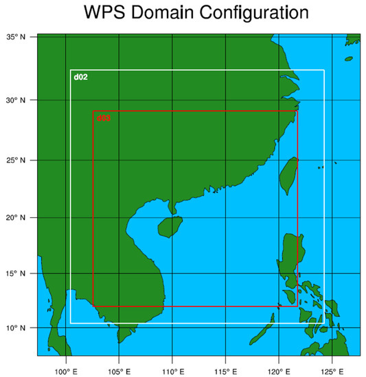
Figure 2.
WRF preprocessing system (WPS) domains of this study, with the innermost domain covering entire South China Sea.
2.3. Methodology
The simulation results are validated by comparing the satellite and in situ datasets. For the analysis purposes, we have obtained long-term temporal resolution data from nine locations (six offshore and three onshore) along the Southern China coast, with the information listed in Table 1 and denoted in Figure 1b. For those offshore locations, three sites along the Southern China coast and the other three sites further interior to the ocean are considered. For onshore locations, three sites at the airports were analyzed. The correlation, root mean square error (RMSE), and the standard deviation were analyzed with the Taylor diagram [59] between different datasets and model simulations. Taylor diagrams bring these statistical parameters together to evaluate the model performance.

Table 1.
Coordinates of the locations used in the analysis.
The interannual variability (IAV) is estimated by the coefficient of variability [60] which is defined as the ratio between interannual standard deviation ( is in years) at any location to the interannual mean ().
We also analyzed the wind power density (WPD), which gives the measure of how much energy is available at any location that can be extracted through a wind turbine [61]
where ρ is the air density (kg m−3), A is the cross-sectional area of the wind turbine (m2) and v is the velocity (m s−1) measured at the height of wind turbine (i.e., 100 m here). Having ρ and A as constant, we can write Equation (2) as
It should be noted that the maximum available wind energy that can be extracted by wind turbines is governed by Betz’s law [62] and it is about 59.3% of the WPD.
3. Results
3.1. Comparison of Surface Winds
The hourly 10 m simulated wind speeds are extracted from the WRF simulations. The 10 m constrain is placed because of available long-term hourly data from the observation. The simulated results are then averaged over a day and used for the analysis. Figure 3 compares the daily average from model results with NOAA integrated surface data for the land and MERRA data for interior oceans. When comparing the simulation results, WRF simulations forced with NCEP-FNL data are represented by WRF-N, WRF simulations forced by ERA-Interim models are represented by WRF-E, and WRF simulations forced with CFSv2 models are represented by WRF-C. In this section, we have taken three locations, one along the onshore (Nanping), one along the coastal China (Hong Kong), and one at 100 km offshore of Quanzhou. Additional locations and their analysis are provided in the Appendix A (Figure A1, Figure A2 and Figure A3). The results in the Appendix A are equally valid. The model output daily averaged wind speed shows a good correlation with the observational data with narrow deviation from the diagonal favoring higher wind speed derived from the simulations. The maximum wind speeds occur in the offshore region (including sites in Appendix A Figure A1, Figure A2 and Figure A3) with overall wind speed ranging from 5 to 20 m s−1. For coastal and interior China, the wind speed is lower with a range from 2 to 10 m s−1. Along the coastal region, WRF-E has lower deviations from the one-to-one line, while WRF-N and WRF-C simulations have a significant positive bias.
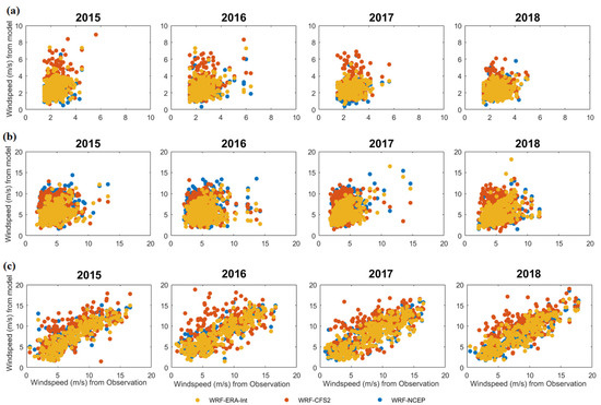
Figure 3.
Daily average wind speed in m s−1 from the models and observations at the locations (a) Nanping, (b) Hong Kong, and (c) offshore Quanzhou.
The RMSE and correlation for the daily wind speed for the entire simulation period at different locations are listed in Table 2 and compared in Figure 4 using Taylor diagrams. In the Taylor diagrams, data from the NOAA surface data are considered as the observation and the simulated results are validated against it. When compared with in situ observation, WRF-E simulations show a better correlation and lower RMSE along the onshore region. For the higher wind speed situations, the WRF-E has 0.5 m s−1 lower RMSE than WRF-N simulations. In most of the locations, WRF-E simulations generally show a better correlation with lower standard deviation and RMSE when compared to the other simulations. Taylor diagrams for additional locations are given in Appendix Figure A4.
Table 2.
Statistics of wind speed at different locations.
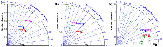
Figure 4.
Taylor diagram for wind speed in m s−1 from the models and observations at the locations (a) Nanping, (b) Hong Kong, and (c) offshore Quanzhou.
Figure 5 compares the monthly mean observed wind speed for different sites with simulations forced by three different initial and boundary conditions. Here, it is noted that the models perform well in simulating the onshore and offshore winds (Figure 5a,b) very well, but at the coastal sea, the models are inefficient in simulating the monthly winds. The monthly variations in the wind speeds are absent in the interior and far-off China but register highly in the coastal regions. The offshore region records the maximum winds in the fall and winter seasons (from October to February), while the remaining months have relatively low wind speeds. In the coastal region, the WRF-E can be seen closely matching the available observational data than the other models. Additional locations are provided in the Appendix Figure A5, Figure A6 and Figure A7.
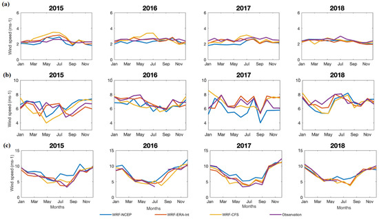
Figure 5.
Monthly averaged wind speed in m s−1 from the models and observations at the locations (a) Nanping, (b) Hong Kong, and (c) offshore Quanzhou.
3.2. Comparison of Wind Direction
The simulated 10 m level wind direction in Hong Kong is compared with the in situ observation for the years 2015 and 2016 (Figure 6). The WRF-N and WRF-E models estimate that most of the strong winds are north and northwestward, which agrees well with the observation. In 2015, the models also reproduce weak eastward wind while observation shows weak eastward and westward winds. In 2016, the WRF-N model reproduces predominantly northward winds, while the WRF-E shows northward predominant and southeastward mild winds. The observed winds are seen predominantly northwards with the low frequent east and west winds. During these two years, the WRF-C simulation fails to reproduce the direction and wind speed and it shows winds are only in the northward direction. The similar analysis for Dongsha island for the years 2015 and 2016 is shown in Figure 7. The simulations are also able to reproduce the observed northeastward winds. The low frequent southwestwards winds are reproduced in WRF-N and WRF-E simulations but absent in WRF-C simulations for both years. Additional analysis through wind rose diagrams for different years are available in Appendix Figure A8 and Figure A9.
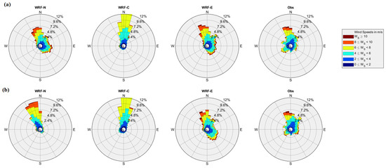
Figure 6.
Wind rose diagram from the models and observations for the years (a) 2015 and (b) 2016 in Hong Kong.
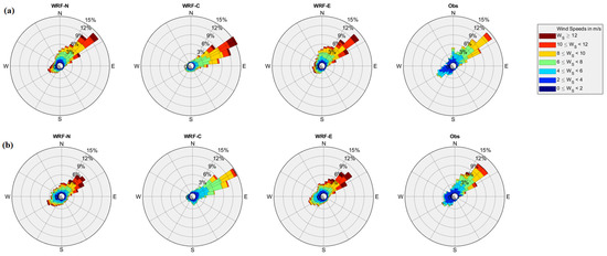
Figure 7.
Wind rose diagram on an hourly timescale from the models and observations for the years (a) 2015 and (b) 2016 in Dongsha Island.
3.3. Comparison of Surface Temperature
For the verification in simulating the surface temperature, we compared the model results to that from MERRA reanalysis datasets for the temperature at the 2 m level, as shown in Figure 8. The WRF-C simulation overestimates the surface temperature while the WRF-N underestimates the same. Figure 8 shows that the simulations are able to capture the temperature variations, with a bias of about 0.5 K for the WRF-E simulations. More scatter plot analyses for temperature are added in Appendix A Figure A10, Figure A11 and Figure A12.
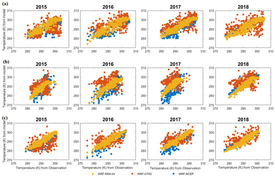
Figure 8.
Daily average temperature in (unit: K) from the models and observations at the locations (a) Nanping, (b) Hong Kong, and (c) offshore Quanzhou.
The RMSE and correlation for the daily average surface temperature for the entire simulation period at different locations are listed in Table 3 and three locations (Nanping, Hong Kong, and offshore Quanzhou) are compared in Figure 9 using Taylor diagrams (additional locations are available in Appendix A Figure A13). WRF-E simulations have higher correlations and smaller standard deviations. It is again noted that the models perform well in interior and offshore China but have lower accuracy in the coastal region. The RMSE of the model simulated temperature is found to be ~1 K in WRF-E model simulations and ~1.5 K in the WRF-N model simulations and the largest in the WRF-C simulations. The correlation between observation and the WRF-N model simulations is 0.7, while that for WRF-E simulations is 0.9 for the Hong Kong region. The WRF-C model overestimates the temperature, the WRF-N underestimates, and WRF-E falls in a good range.
Table 3.
Statistics of temperature at different locations.
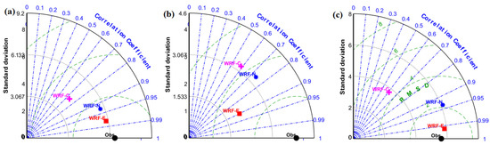
Figure 9.
Taylor diagram for temperature in K from the models and observations at the locations (a) Nanping, (b) Hong Kong, and (c) offshore Quanzhou.
3.4. Comparison of Seasonal Winds
For the South China Sea, the seasons are defined as follows: summer comprises June–August, autumn in September–November, winter in December–February, followed by spring in March–May. The seasonal variability in wind speed over the South China Sea and the surrounding regions are mainly influenced by the Asian monsoon and the orography of the region. Figure 10 compares the seasonal wind speeds from the models with those from satellite QuikSCAT observation and other reanalysis datasets. The winds are calm during the summer monsoon while they reach their maximum during the winter monsoonal period. Both the WRF-N and WRF-E simulations are able to reproduce the seasonal wind pattern with maximum winds occurring along the Taiwan Strait. The southern coast of China receives the strongest winds with the persistent high reaching above 15 m s−1 in winter. These winds start at the end of summer and continue till the end of winter. The coastal region between Hainan and Taiwan are excellent locations for wind farm settings due to the rich wind resource and shallow bathymetry.
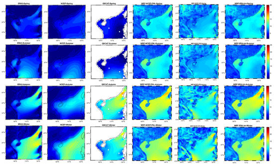
Figure 10.
Average seasonal wind speed in m s−1 from the models and observations for all the seasons along the study area. Spring is shown in first row, summer in second row, autumn in third row and winter in fourth row. The first column represents ERA5 data, second column from NCEP Reanalysis 2, third column from QuikScat, fourth column from WRF-N simulations, fifth from WRF-C simulations and sixth from WRF-E simulations.
3.5. Interannual Variations and Wind Power Density
To optimize the windfarm setting, the interannual variations (IAV) of the wind speed and the average wind power density in terms of cubic windspeed using Equation (3) are examined. Since the WRF-E simulation has a better performance in reproducing the wind field characteristics, the following analysis will be mainly based on the WRF-E results. Figure 11a shows that the IAVs along the coastal region are low (<2%) and hence these regions act as an excellent region for long-term offshore wind energy investments. The open ocean has the highest interannual variations. Along the coastal regions, Taiwan Strait has the maximum average wind power density and minimum interannual variations. This region acts as an excellent region to obtain wind energy in the South China Sea. This region is also identified as one of the best regions over the globe to extract wind energy in the range higher than 600 W m−2 [63,64]. Followed by the Taiwan strait, the regions around Guangdong province and the Hunan province also share some of the highest wind power density amidst lower interannual variations in the South China Sea.
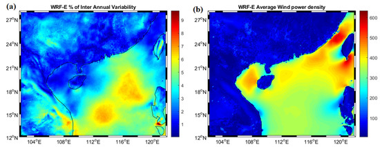
Figure 11.
(a) Interannual variability and (b) average wind power density (m3 s−3) for the year 2015–2018 from WRF-E simulations.
4. Discussions
The main difference between analysis (NCEP-FNL) and reanalysis (ERA-Interim and NCEP-CFSv2) data is the amount of observational data that enters in the data assimilation step. For example, the analysis data are created very quickly while reanalysis data takes more than 3–4 days. Therefore, biases are corrected, and more satellite data enters the creation of reanalysis data [28]. Reanalysis data is dependent on the underlying forecast models, data input sources, and assimilation systems [65]. The main advantage of the ERA-Interim data is the inclusion of a four-dimensional variational analysis (4D-Var) assimilation system of observed data, while the other reanalysis data have the 3D-Var assimilation system. The 4D-Var assimilation system reduces the various biases in the model output. The boundary conditions used by these reanalyses are different. For example, SSTs for the NCEP-CFSv2 model are generated by an atmosphere-ocean coupling model, while the ERA-Interim is run with observed SSTs [66].
Among the three reanalysis datasets used to simulate the wind resources along South China Sea, ERA-Interim forced models produced the best results. However, along the coastal regions, even ERA-Interim forced data could not reproduce the wind speed and its evolution well. This mainly happens because the interactions between ocean and atmosphere near coastal regions are complex and a standalone atmosphere model will not be able to capture them. In future, this modeling approach can be extended with coupled numerical models, where there exists constant interchange of data between atmosphere and oceans, can be used to improve the wind resource estimations. Further, the innermost domain of the current study is in the range of 4 km which is considered coarser for wind farms as they require sub-kilometer scale wind resource estimations. With this study as the base, more studies can be built by selecting the region of interest and performing higher resolution modeling in a sub-kilometer scale.
With ERA-Interim data providing the best wind resource estimations over South China Sea, the sensitivity of WRF model can be further analyzed by varying different parameterization schemes for planetary boundary layer and land surface models. The parametrization schemes for this study are chosen based on the literatures but different combination of the schemes can provide different and improved results which can be further explored.
5. Summary and Conclusions
In this study, the high-resolution WRF simulations over the South China Sea and surrounding regions are conducted to study the sensitivity of various initial and boundary conditions in simulating the near-surface wind and temperature fields. Three state-of-the-art reanalysis datasets (NCEP-FNL, ERA-Interim, and NCEP CFSv2) are used as the forcing data for the numerical simulations between 2015 and 2018. The model results are analyzed and compared with various observed datasets.
ERA-Interim-forced simulations performed well in comparison with other datasets. The error from the simulations is lowest in the WRF-E models followed by WRF-N and WRF-C simulations when comparing daily wind speeds. Over most of the locations considered, WRF-E has a better correlation and lower RMSE among the three. The monthly variations are also captured by the simulations along the coastal region but not for the open ocean.
The simulations are also able to reproduce the wind directions along the coastal China, with WRF-E and WRF-N simulations performing better followed by WRF-C. In a seasonal characteristics of wind speed, WRF-E and WRF-N performed well while WRF-C could not reproduce high wind speeds in the open ocean. The near-surface temperature simulations show that the models are able to capture the variations with small deviation from the observation data. Of all the models, the WRF-E simulations outputs are good when compared with other simulations for temperature. The WRF-N has a negative temperature bias, while the WRF-C has a positive bias in some regions. Seasonal variations show that autumn and winter provide excellent conditions to extract wind energy along the South China Sea. Furthermore, interannual variability of windspeed shows that the wind energy near the onshore and coastal region is stable, with the coastal regions registering maximum wind power density over the South China Sea. These coastal regions are excellent grounds for future wind power investments as they have low interannual variability. Overall, WRF forced with ERA-Interim data provided the best simulations followed by NCEP Final analysis and CFSv2 data for the South China Sea, which indicates that the ERA-Interim data can be used as the best initial and boundary data for further numerical modeling in this region.
Author Contributions
Conceptualization, T.X. and Y.-F.M.; numerical modeling, visualization, and original draft preparation, A.T.; writing—review and editing, T.X., Y.-F.M. and L.-P.W.; funding acquisition, L.-P.W. All authors have read and agreed to the published version of the manuscript.
Funding
This work has been supported by the Southern Marine Science and Engineering Guangdong Laboratory (Guangzhou) (GML2019ZD0103), the National Natural Science Foundation of China (91852205, 91741101, 11961131006, 42075071, and 42075078), NSFC Basic Science Center Program (11988102), Guangdong Provincial Key Laboratory of Turbulence Research and Applications (2019B21203001), Guangdong-Hong Kong-Macao Joint Laboratory for Data-Driven Fluid Mechanics and Engineering Applications (2020B1212030001), and Shenzhen Science and Technology Program (KQTD20180411143441009).
Institutional Review Board Statement
Not applicable.
Informed Consent Statement
Not applicable.
Data Availability Statement
The data used in this manuscript are downloaded from the following open websites: ERA-Interim: https://rda.ucar.edu/datasets/ds627.0, accessed on 25 May2021. NCEP-FNL: https://rda.ucar.edu/datasets/ds083.2, accessed on 25 May2021. NCEP-CFSv2: https://rda.ucar.edu/datasets/ds094.0, accessed on 25 May2021. ETOPO2: https://rda.ucar.edu/datasets/ds759.3, accessed on 25 October 2020. MERRA: https://gmao.gsfc.nasa.gov/reanalysis/MERRA-2/, accessed on 20 October 2020. NOAA: https://www.ncei.noaa.gov/products/land-based-station/integrated-surface-database, accessed on 20 October 2020. ECMWF-ERA5: https://cds.climate.copernicus.eu/cdsapp#!/dataset/reanalysis-era5-pressure-levels-monthlymeans?tab=overview, accessed on 15 January 2021. NCEP Reanalysis2: https://psl.noaa.gov/data/gridded/data.ncep.reanalysis2.gaussian.html, accessed on 13 February 2021. QuikScat: https://www.remss.com, accessed on 15 January 2021. Computing resources are provided by the Center for Computational Science and Engineering of Southern University of Science and Technology.
Acknowledgments
We would like to acknowledge the high-performance computing support from “TaiYi” provided by SUSTech Center for Computational Science & Engineering.
Conflicts of Interest
The authors declare no conflict of interest.
Appendix A
This appendix provides additional figures to the validation of model results.
Figure A1.
Daily average wind speed in m s−1 from the models and observations at the onshore locations (a) Shaoguan, (b) Nanping, and (c) Ganzhou.
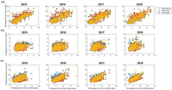
Figure A2.
Daily average wind speed in m s−1 from the models and observations at the offshore locations (a) Quanzhou, (b) Shanwei, and (c) Nansan.
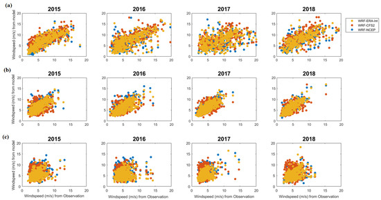
Figure A3.
Daily average wind speed in m s−1 from the models and observations at the locations (a) Dongsha, (b) Zhanjiang, and (c) Hong Kong.
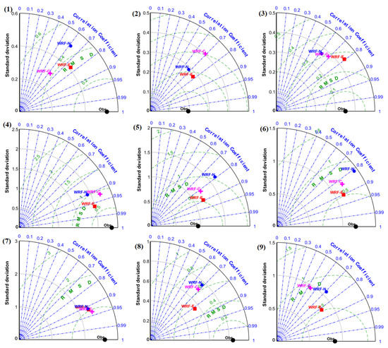
Figure A4.
Taylor diagram for wind speed in m s−1 from the models and observations at the locations (1) Shaoguan, (2) Nanping, (3) Ganzhou, (4) Offshore Quanzhou, (5) Offshore Shanwei, (6) Offshore Nansan, (7) Dongsha, (8) Zhanjiang and (9) Hong Kong.
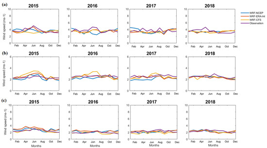
Figure A5.
Monthly averaged wind speed in m s−1 from the models and observations at the onshore locations (a) Shaoguan, (b) Nanping, and (c) Ganzhou.
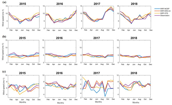
Figure A6.
Monthly averaged wind speed in m s−1 from the models and observations at the offshore locations (a) Quanzhou, (b) Shanwei, and (c) Nansan.
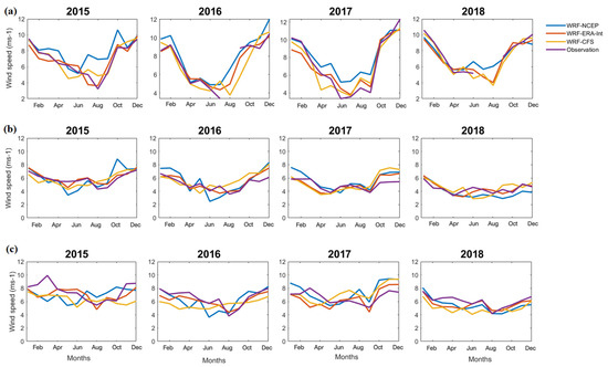
Figure A7.
Monthly averaged wind speed in m s−1 from the models and observations at the locations (a) Dongsha, (b) Zhanjiang, and (c) Hong Kong.
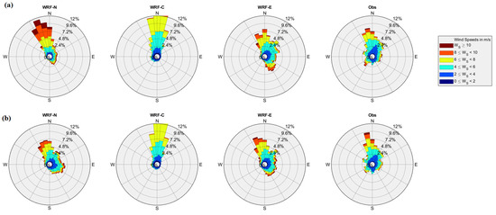
Figure A8.
Wind rose diagram on an hourly timescale from the models and observations for the years (a) 2017 (top) and (b) 2018 (bottom) at Hong Kong.
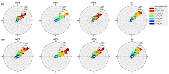
Figure A9.
Wind rose diagram on an hourly timescale from the models and observations for the years (a) 2017 (top) and (b) 2018 (bottom) at Dongsha Dao.
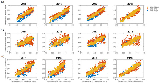
Figure A10.
Daily average temperature in K from the models and observations at the onshore locations (a) Shaoguan, (b) Nanping, and (c) Ganzhou.
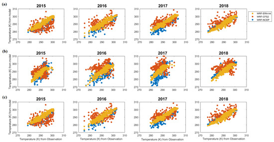
Figure A11.
Daily average temperature in K from the models and observations at the offshore locations (a) Quanzhou, (b) Shanwei, and (c) Nansan.
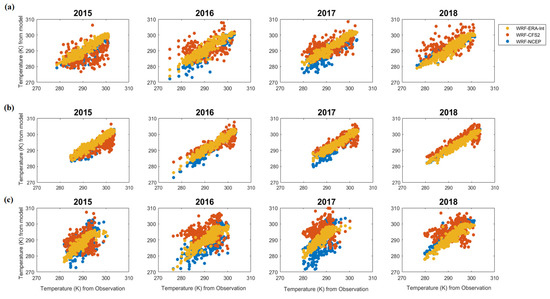
Figure A12.
Daily average temperature in K from the models and observations at the locations (a) Dongsha, (b) Zhanjiang, and (c) Hong Kong.
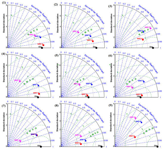
Figure A13.
Taylor diagram for temperature in K from the models and observations at the locations (1) Shaoguan, (2) Nanping, (3) Ganzhou, (4) Offshore Quanzhou, (5) Offshore Shanwei, (6) Offshore Nansan, (7) Dongsha, (8) Zhanjiang and (9) Hong Kong.
References
- Global Energy Statistical Yearbook. 2019. Available online: https://yearbook.enerdata.net/total-energy/world-energy-intensity-gdp-data.html (accessed on 30 September 2021).
- “2020 Q2 Electricity & Other Energy Statistics”. China Energy Portal. Available online: https://chinaenergyportal.org/2020-q2-electricity-other-energy-statistics (accessed on 25 April 2021).
- Yang, J.; Gao, S. Analysis: China Adds to UHV Network to Transfer Surplus Wind Energy. Available online: https://www.windpowermonthly.com/article/1361466/analysis-china-adds-uhv-network-transfer-surplus-wind-energy (accessed on 28 August 2020).
- Zhang, S.; Wei, J.; Chen, X.; Zhao, Y. China in global wind power development: Role, status and impact. Renew. Sustain. Energy Rev. 2020, 127, 109881. [Google Scholar] [CrossRef]
- Yang, J.; Liu, Q.; Li, X.; Cui, X. Overview of wind power in China: Status and future. Sustainability 2017, 9, 1454. [Google Scholar] [CrossRef] [Green Version]
- Wan, Y.; Fan, C.; Dai, Y.; Li, L.; Sun, W.; Zhou, P.; Qu, X. Assessment of the joint development potential of wave and wind energy in the South China Sea. Energies 2018, 11, 398. [Google Scholar] [CrossRef] [Green Version]
- Zheng, C.; Zhuang, H.; Li, X.; Li, X. Wind energy and wave energy resources assessment in the East China Sea and South China Sea. Sci. China Technol. Sci. 2012, 55, 163–173. [Google Scholar] [CrossRef]
- Zheng, C.W.; Pan, J.; Li, J.X. Assessing the China Sea wind energy and wave energy resources from 1988 to 2009. Ocean. Eng. 2013, 65, 39–48. [Google Scholar] [CrossRef]
- Chang, R.; Zhu, R.; Badger, M.; Hasager, C.B.; Xing, X.; Jiang, Y. Offshore wind resources assessment from multiple satellite data and WRF modeling over South China Sea. Remote Sens. 2015, 7, 467–487. [Google Scholar] [CrossRef] [Green Version]
- Hashim, F.E.; Peyre, O.; Lapok, S.J.; Yaakob, O.; Din, A.H.M. Offshore wind energy resource assessment in Malaysia with satellite altimetry. J. Sustain. Sci. Manag. 2020, 15, 111–124. [Google Scholar] [CrossRef]
- Alifdini, I.; Shimada, T.; Wirasatriya, A. Seasonal distribution and variability of surface winds in the Indonesian seas using scatterometer and reanalysis data. Int. J. Climatol. 2021, 41, 4825–4843. [Google Scholar] [CrossRef]
- Nezhad, M.M.; Neshat, M.; Heydari, A.; Razmjoo, A.; Piras, G.; Garcia, D.A. A new methodology for offshore wind speed assessment integrating Sentinel-1, ERA-Interim and in-situ measurement. Renew. Energy 2021, 172, 1301–1313. [Google Scholar] [CrossRef]
- Chen, X.; Pan, D.; He, X.; Bai, Y.; Wang, Y.; Zhu, Q. Seasonal and interannual variability of sea surface wind over the China seas and its adjacent ocean from QuikSCAT and ASCAT data during 2000–2011. In Remote Sensing of the Ocean, Sea Ice, Coastal Waters, and Large Water Regions, Proceedings of the SPIE Remote Sensing, 2012, Edinburgh, UK, 24–27 September 2012; SPIE: Bellingham, WA, USA, 2012; Volume 8532, p. 853214. [Google Scholar] [CrossRef]
- Jiang, D.; Zhuang, D.; Huang, Y.; Wang, J.; Fu, J. Evaluating the spatio-temporal variation of China’s offshore wind resources based on remotely sensed wind field data. Renew. Sustain. Energy Rev. 2013, 24, 142–148. [Google Scholar] [CrossRef]
- Sun, S.; Fang, Y.; Zu, Y.; Liu, B.; Samah, A.A. Seasonal characteristics of mesoscale coupling between the sea surface temperature and wind speed in the South China Sea. J. Clim. 2020, 33, 625–638. [Google Scholar] [CrossRef]
- Larsén, X.G.; Mann, J. Extreme winds from the NCEP/NCAR Reanalysis Data. Wind. Energy 2009, 12, 556–573. [Google Scholar] [CrossRef]
- Gallego, C.; Pinson, P.; Madsen, H.; Costa, A.; Cuerva, A. Influence of local wind speed and direction on wind power dynamics—Application to offshore very short-term forecasting. Appl. Energy 2011, 88, 4087–4096. [Google Scholar] [CrossRef] [Green Version]
- Jiménez, B.; Durante, F.; Lange, B.; Kreutzer, T.; Tambke, J. Offshore wind resource assessment with WAsP and MM5: Comparative study for the German Bight. Wind Energy 2007, 10, 121–134. [Google Scholar] [CrossRef]
- Wallcraft, A.J.; Kara, A.B.; Barron, C.N.; Metzger, E.J.; Pauley, R.L.; Bourassa, M.A. Comparisons of monthly mean 10 m wind speeds from satellites and NWP products over the global ocean. J. Geophys. Res. 2009, 114, 16109–16114. [Google Scholar] [CrossRef] [Green Version]
- Hasager, C.B.; Astrup, P.; Zhu, R.; Chang, R.; Badger, M.; Hahmann, A.N. Quarter-century offshore winds from SSM/I and WRF in the North Sea and South China Sea. Remote Sens. 2016, 8, 769. [Google Scholar] [CrossRef] [Green Version]
- Wang, Z.; Duan, C.; Dong, S. Long-term wind and wave energy resource assessment in the South China sea based on 30-year hindcast data. Ocean. Eng. 2018, 163, 58–75. [Google Scholar] [CrossRef]
- Huang, Y.; Liu, Y.; Liu, Y.; Li, H.; Knievel, J.C. Mechanisms for a record-breaking rainfall in the coastal metropolitan city of Guangzhou, China: Observation analysis and nested very large eddy simulation with the WRF model. J. Geophys. Res. Atmos. 2019, 124, 1370–1391. [Google Scholar] [CrossRef]
- Pan, L.; Liu, Y.; Roux, G.; Cheng, W.; Liu, Y.; Hu, J.; Jin, S.; Feng, S.; Du, J.; Peng, L. Seasonal variation of the surface wind forecast performance of the high-resolution WRF-RTFDDA system over China. Atmos. Res. 2021, 259, 105673. [Google Scholar] [CrossRef]
- Zhang, C.; He, J.; Lai, X.; Liu, Y.; Che, H.; Gong, S. The impact of the variation in weather and weason on WRF dynamical downscaling in the Pearl River Delta region. Atmosphere 2021, 12, 409. [Google Scholar] [CrossRef]
- National Centers for Environmental Prediction/National Weather Service/NOAA/U.S. Department of Commerce. 2000, Updated Daily. NCEP FNL Operational Model Global Tropospheric Analyses, continuing from July 1999. Research Data Archive at the National Center for Atmospheric Research, Computational and Information Systems Laboratory. Available online: https://rda.ucar.edu/datasets/ds083.2/ (accessed on 25 May 2021). [CrossRef]
- European Centre for Medium-Range Weather Forecasts. 2009, Updated Monthly. ERA-Interim Project. Research Data Archive at the National Center for Atmospheric Research, Computational and Information Systems Laboratory. Available online: https://rda.ucar.edu/datasets/ds627.0/ (accessed on 25 May 2021). [CrossRef]
- Saha, S.; Moorthi, S.; Wu, X.; Wang, J.; Nadiga, S. NCEP Climate Forecast System Version 2 (CFSv2) 6-Hourly Products. Research Data Archive at the National Center for Atmospheric Research, Computational and Information Systems Laboratory. 2011. Available online: https://rda.ucar.edu/datasets/ds094.0/ (accessed on 25 May 2021). [CrossRef]
- Carvalho, D.; Rocha, A.; Gómez-Gesteira, M.; Santos, C.S. Offshore wind energy resource simulation forced by different reanalyses: Comparison with observed data in the Iberian Peninsula. Appl. Energy 2014, 134, 57–64. [Google Scholar] [CrossRef]
- Giannakopoulou, E.M.; Nhili, R. WRF model methodology for offshore wind energy applications. Adv. Meteorol. 2014, 2014, 319819. [Google Scholar] [CrossRef] [Green Version]
- Lorenz, T.; Barstad, I. A dynamical downscaling of ERA-Interim in the North Sea using WRF with a 3 km grid—For wind resource applications. Wind Energy 2016, 19, 1945–1959. [Google Scholar] [CrossRef]
- Mattar, C.; Borvarán, D. Offshore wind power simulation by using WRF in the central coast of Chile. Renew. Energy 2016, 94, 22–31. [Google Scholar] [CrossRef]
- Kryza, M.; Wałaszek, K.; Ojrzyńska, H.; Szymanowski, M.; Werner, M.; Dore, A.J. High-resolution dynamical downscaling of ERA-interim using the WRF regional climate model for the area of Poland. Part 1: Model configuration and statistical evaluation for the 1981–2010 Period. Pure Appl. Geophys. 2017, 174, 511–526. [Google Scholar] [CrossRef] [Green Version]
- Li, X.; Gao, Y.; Pan, Y.; Xu, Y. Evaluation of near-surface wind speed simulations over the Tibetan Plateau from three dynamical downscalings based on WRF model. Theor. Appl. Climatol. 2018, 134, 1399–1411. [Google Scholar] [CrossRef]
- Chadee, X.T.; Seegobin, N.R.; Clarke, R.M. Optimizing the Weather Research and Forecasting (WRF) model for mapping the near-surface wind resources over the Southernmost Caribbean Islands of Trinidad and Tobago. Energies 2017, 10, 931. [Google Scholar] [CrossRef] [Green Version]
- De Araujo, J.M.S. WRF wind speed simulation and SAM wind energy estimation: A case study in Dili Timor Leste. IEEE Access 2019, 7, 35382–35393. [Google Scholar] [CrossRef]
- Lakshmi, D.D.; Murty, P.L.N.; Bhaskaran, P.K.; Sahoo, B.; Kumar, T.S.; Shenoi, S.S.C.; Srikanth, A.S. Performance of WRF-ARW winds on computed storm surge using hydodynamic model for Phailin and Hudhud cyclones. Ocean. Eng. 2017, 131, 135–148. [Google Scholar] [CrossRef]
- Anandh, T.S.; Das, B.K.; Kuttippurath, J.; Chakraborty, A. A coupled model analyses on the interaction between oceanic eddies and tropical cyclones over the Bay of Bengal. Ocean. Dyn. 2020, 70, 327–337. [Google Scholar] [CrossRef]
- Chen, C.; Sasa, K.; Ohsawa, T.; Kashiwagi, M.; Prpić-Oršić, J.; Mizojiri, T. Comparative assessment of NCEP and ECMWF global datasets and numerical approaches on rough sea ship navigation based on numerical simulation and shipboard measurements. Appl. Ocean. Res. 2020, 101, 102219. [Google Scholar] [CrossRef]
- Devanand, A.; Roxy, M.K.; Ghosh, S. Coupled land-atmosphere regional model reduces dry bias in Indian Summer Monsoon rainfall simulated by CFSv2. Geophys. Res. Lett. 2018, 45, 2476–2486. [Google Scholar] [CrossRef]
- Diaz, L.R.; Mollmann, R.A.; Muchow, G.B.; Käfer, P.S.; Rocha, N.S.; Kaiser, E.A.; Costa, S.T.L.; Hallal, G.P.; Alves, R.C.M.; Rolim, S.B.A. Analysis of an extratropical cyclone in the Southwest Atlantic: WRF model boundary conditions sensitivity. In Proceedings of the International Archives of the Photogrammetry, Remote Sensing and Spatial Information Sciences, Santiago, Chile, 22–26 March 2020; XLII-3/W12-2020. pp. 107–112. [Google Scholar] [CrossRef]
- Gippius, F.N.; Myslenkov, S.A. Black Sea wind wave climate with a focus on coastal regions. Ocean. Eng. 2020, 218, 108199. [Google Scholar] [CrossRef]
- Im, E.S.; Ha, S.; Qiu, L.; Hur, J.; Jo, S.; Shim, K.M. An evaluation of temperature-based agricultural indices over Korea from the high-resolution WRF simulation. Front. Earth Sci. 2021, 9, 357. [Google Scholar] [CrossRef]
- Samanta, D.; Hameed, S.N.; Jin, D.; Thilakan, V.; Ganai, M.; Rao, S.A.; Deshpande, M. Impact of a narrow coastal Bay of Bengal Sea surface temperature front on an Indian summer monsoon simulation. Sci. Rep. 2018, 8, 17694. [Google Scholar] [CrossRef] [Green Version]
- Rienecker, M.M.; Suarez, M.J.; Gelaro, R.; Todling, R.; Bacmeister, J.; Liu, E.; Bosilovich, M.G.; Schubert, S.D.; Takacs, L.; Kim, G.; et al. MERRA: NASA’s Modern-Era Retrospective Analysis for Research and Applications. J. Clim. 2011, 24, 3624–3648. [Google Scholar] [CrossRef]
- Bentamy, A.; Fillon, D.C. Gridded surface wind fields from Metop/ASCAT measurements. Int. J. Remote Sens. 2012, 33, 1729–1754. [Google Scholar] [CrossRef] [Green Version]
- Gruber, K.; Regner, P.; Wehrle, S.; Zeyringer, M.; Schmidt, J. Towards global validation of wind power simulations: A multi-country assessment of wind power simulation from MERRA-2 and ERA-5 reanalyses bias-corrected with the global wind atlas. Energy 2022, 238, 121520. [Google Scholar] [CrossRef]
- Olauson, J.; Bergkvist, M. Modelling the Swedish wind power production using MERRA reanalysis data. Renew. Energy 2015, 76, 717–725. [Google Scholar] [CrossRef]
- Global Surface Hourly [Integrated Surface Dataset]. NOAA National Centers for Environmental Information, 2011. Available online: https://journals.ametsoc.org/view/journals/bams/92/6/2011bams3015_1.xml (accessed on 20 October 2020). [CrossRef]
- National Geophysical Data Center/NESDIS/NOAA/U.S. Department of Commerce. ETOPO2, Global 2 Arc-minute Ocean Depth and Land Elevation from the US National Geophysical Data Center (NGDC). Research Data Archive at the National Center for Atmospheric Research, Computational and Information Systems Laboratory, 2001. Available online: https://rda.ucar.edu/datasets/ds759.3/ (accessed on 25 October 2020). [CrossRef]
- Copernicus Climate Change Service (C3S): ERA5: Fifth Generation of ECMWF Atmospheric Reanalyses of the Global Climate. Copernicus Climate Change Service Climate Data Store (CDS), 2017. Available online: https://cds.climate.copernicus.eu/cdsapp (accessed on 15 January 2021).
- Kanamitsu, M.; Ebisuzaki, W.; Woollen, J.; Yang, S.K.; Hnilo, J.J.; Fiorino, M.; Potter, G.L. NCEP-DOE AMIP-II Reanalysis (R-2). Bull. Am. Meteorol. Soc. 2002, 83, 1631–1643. [Google Scholar] [CrossRef]
- Risien, C.M.; Chelton, D.B. A global climatology of surface wind and wind stress fields from eight years of QuikSCAT scatterometer data. J. Phys. Oceanogr. 2008, 38, 2379–2413. [Google Scholar] [CrossRef]
- Skamarock, W.C.; Klemp, J.B.; Dudhia, J.; Gill, D.O.; Liu, Z.; Berner, J.; Wang, W.; Powers, J.G.; Duda, M.G.; Barker, D.M.; et al. A Description of the Advanced Research WRF Model Version 4; National Center for Atmospheric Research: Boulder, CO, USA, 2019; p. 145. [Google Scholar]
- Mlawer, E.J.; Taubman, S.J.; Brown, P.D.; Iacono, M.J.; Clough, S.A. Radiative transfer for inhomogeneous atmospheres: RRTM, a validated correlated-k model for the longwave. J. Geophys. Res. 1997, 102, 16663–16682. [Google Scholar] [CrossRef] [Green Version]
- Dudhia, J. Numerical study of convection observed during the winter monsoon experiment using a mesoscale two-dimensional model. J. Atmos. Sci. 1989, 46, 3077–3107. [Google Scholar] [CrossRef]
- Nakanishi, M.; Niino, H. An Improved Mellor–Yamada Level-3 Model: Its Numerical Stability and Application to a Regional Prediction of Advection Fog. Bound.-Layer Meteorol. 2006, 119, 397–407. [Google Scholar] [CrossRef]
- Kain, J.S. The Kain–Fritsch convective parameterization: An update. J. Appl. Meteorol. 2004, 43, 170–181. [Google Scholar] [CrossRef] [Green Version]
- Morrison, H.; Thompson, G.; Tatarskii, V. Impact of cloud microphysics on the development of trailing stratiform precipitation in a simulated squall line: Comparison of one-and two-moment schemes. Mon. Weather. Rev. 2009, 137, 991–1007. [Google Scholar] [CrossRef] [Green Version]
- Taylor, K.E. Summarizing multiple aspects of model performance in a single diagram. J. Geophys. Res. Atmos. 2001, 106, 7183–7192. [Google Scholar] [CrossRef]
- Brower, M.C. Wind Resource assessment: A Practical Guide to Developing a Wind Project; John Wiley & Sons, Inc.: Hoboken, NJ, USA, 2012; p. 280. ISBN 9781118249864. [Google Scholar]
- Manwell, J.F.; McGowan, J.G.; Rogers, A.L. Wind Energy Explained: Theory, Design and Application, 2nd ed.; John Wiley & Sons, Inc.: Washington, DC, USA, 2010; p. 689. ISBN 978-0470015001. [Google Scholar]
- Betz, A. Introduction to the Theory of Flow Machines; Permagon Press: Oxford, UK, 1966; ISBN 9781483180908. [Google Scholar]
- Zheng, C.W.; Li, X.Y.; Luo, X.; Chen, X.; Qian, Y.H.; Zhang, Z.H.; Gao, Z.S.; Du, Z.B.; Gao, Y.B.; Chen, Y.G. Projection of future global offshore wind energy resources using CMIP data. Atmos.-Ocean 2019, 57, 134–148. [Google Scholar] [CrossRef]
- Soares, P.M.; Lima, D.C.; Nogueira, M. Global offshore wind energy resources using the new ERA-5 reanalysis. Environ. Res. Lett. 2020, 15, 1040a2. [Google Scholar] [CrossRef]
- Xian, T.; Homeyer, C.R. Global tropopause altitudes in radiosondes and reanalyses. Atmos. Chem. Phys. 2019, 19, 5661–5678. [Google Scholar] [CrossRef] [Green Version]
- Fujiwara, M.; Wright, J.S.; Manney, G.L.; Gray, L.J.; Anstey, J.; Birner, T.; Davis, S.; Gerber, E.P.; Harvey, V.L.; Hegglin, M.I.; et al. Introduction to the SPARC Reanalysis Intercomparison Project (S-RIP) and overview of the reanalysis systems. Atmos. Chem. Phys. 2017, 17, 1417–1452. [Google Scholar] [CrossRef] [Green Version]
Publisher’s Note: MDPI stays neutral with regard to jurisdictional claims in published maps and institutional affiliations. |
© 2022 by the authors. Licensee MDPI, Basel, Switzerland. This article is an open access article distributed under the terms and conditions of the Creative Commons Attribution (CC BY) license (https://creativecommons.org/licenses/by/4.0/).