Innovative Trend Analysis of High-Altitude Climatology of Kashmir Valley, North-West Himalayas

Abstract

This paper investigates the annual and seasonal variations in the minimum and maximum air temperature (T_min and T_max) and precipitation over Kashmir valley, Northwestern Himalayas from 1980–2019 by using the innovative trend analysis (ITA), Mann-Kendall (MK), and Sen’s slope estimator methods. The results indicated that the annual and seasonal T_min and T_max are increasing for all the six climatic stations, whereas four of them exhibit significant increasing trends at (α = 0.05). Moreover, this increase in T_min and T_max was found more pronounced at higher altitude stations, i.e., Pahalgam (2650 m asl) and Gulmarg (2740 m asl). The annual and seasonal precipitation patterns for all climatic stations showed downward trends. For instance, Gulmarg station exhibited a significant downward trend for the annual, spring, and winter seasons (α = 0.05). Whereas, Qazigund showed a significant downward trend for the annual and spring seasons (α = 0.05). The overall analysis revealed that the increased T_min and T_max trends during the winter season are one of the reasons behind the early onset of melting of snow and the corresponding spring season. Furthermore, the observed decreased precipitation trends could result in making the region vulnerable towards drier climatic extremes. Such changes in the region’s hydro-meteorological processes shall have severe implications on the delicate ecological balance of the fragile environment of the Kashmir valley.

1. Introduction

Climate change is a natural phenomenon, though extensive research indicates that the anthropogenic activities in the 20th century are one of the major reasons for the temperature increase [1,2,3]. Increasing air temperatures and fluctuating precipitation patterns have gained a lot of attention in recent years because of their importance in understanding the climate change of any region [4,5]. An average increase in air temperature of 0.74 °C has been reported worldwide over the next 100 years [6]. In contrast to global predictions, the estimations of regional climate change rates differ due to differing methodology and datasets used to estimate future climate change [7,8,9].

Precipitation and temperature are considered key climatic variables affecting the spatiotemporal patterns of regional water resources availability [10,11]. Numerous studies have shown that assessing the implications of climate change on regional economic development, agriculture, and human society requires measuring fluctuations in regional air temperature and precipitation [12,13,14,15]. The most significant parameters in hydrometeorology are to evaluate a region’s climate and estimate the consequences of changing climate, which are the air temperature and precipitation [16].

In recent years, substantial research has been carried out to quantify the climate change consequences by identifying the precipitation and temperature trends at various spatiotemporal scales in order to regulate regional resources of water and related hazards [17]. Significant warming trends with a magnitude of 0.16 °C per decade in air temperature were reported during the 20th century over the Tibetan Plateau [18,19,20]. According to [21].

According to Shrestha and Devkota (2010), in most regions of the Hind-Kush Himalayan (HKH), the warming rate is higher in the winter compared to other seasons [22]. In the last few decades, annual and winter precipitation has increased over the Tibetan Plateau and Indus basin. However, in these regions, an incoherent spatial pattern was witnessed for long-term precipitation variability [23]. Several studies have used methodologies to evaluate the temperature and precipitation variations, such as Mann-Kendall (MK) test, Sen’s slope estimator, linear regression (LR), and Spearman’s rho (SR) tests [24]. However, MK test is considered as the most common method used and has been applied in many regions worldwide to detect the changes in the hydro-meteorological variables. The MK test was employed by [25] to examine annual daily maximum precipitation trends and showed a significant increase. Pingale et al. (2014) examined the spatiotemporal mean and extreme rainfall and temperature trends using the MK test and Sen’s slope estimator and found equally positive and negative trends for Rajasthan state urban centres [26]. Using LR and the SR tests [27] evaluated the significant upward trends for heatwaves and air temperatures in northwest Mexico. Gemmer et al. (2011) for observing the spatiotemporal characteristics for trends of rainfall used the MK test and found that while some stations showed annual trends in rainfall, monthly rainfall time series showed significant positive and negative trends in entire China’s Zhujiang River Basin [28]. In another study, the results of the precipitation and temperature trend analysis were used to manage the scarce water resources of such regions for future water resource management development [29].

Few studies have been carried out in the Kashmir valley by using traditional statistical tests for trend analysis in hydro-meteorological data. Gujree et al. (2017), using Sen’s slope estimator and MK test analyzed the spatial variability of precipitation and temperature extremes [30]. They showed that areas in plains exhibited an upward trend in T_max extremes, while in the near future the mountain areas may showcase more extreme events in T_min and precipitation. Shafiq et al. (2019) assessed the changing trends of precipitation and air temperature variables using the non-parametric tests in the Kashmir valley at various elevation zones [31]. Dad et al. (2021) examined the significance of trends and estimated the magnitude of trends in air temperature and precipitation on annual, seasonal, and monthly scales for all six meteorological stations positioned throughout the Kashmir valley employed non-parametric method. Ahmad et al. (2021) used non-parametric tests to assess the trend significance of air temperature and precipitation for the whole Kashmir valley [32]. Zaz et al. (2019) used statistical tests, such as Student’s test, cumulative deviation, MK, and LR to examine the annual and seasonal precipitation and temperature changes in the six meteorological stations of the Kashmir valley [33].

However, traditional trend analysis methods can only detect the monotonic trends through pure statistical calculations and cannot identify the trends in different subcategories of the time series [34]. The innovative trend analysis (ITA) technique had been widely utilized to check trends predicted by existing methods and identify unseen trends in high, medium, and low-value categories utilizing springy graphical tools [17,34]. ITA is an intuitive and straightforward method that can be applied irrespective of distribution assumptions to identify trends in various time series subcategories [35]. In many parts of the world ITA has been used for investigating the hidden trends in hydro-meteorological variables. Ay and Kisi [36] carried out ITA-based trend analysis at six different provinces of Turkey for monthly precipitation and observed significantly upward trends at Trabzon and Samsun regions along with other four regions that were found insignificant. Similarly, Elouissi et al. [35] used this ITA method for assessing monthly precipitation to conduct trend analysis for 25 stations and observed a downward trend towards the northern parts and an upward trend towards the southern parts of the Macta watershed, Algeria. Tosunoglu and Kisi [37] analyzed drought variables for nine stations by means of the modified ITA and MK tests. Moreover, the results showed that the MK test depicted trendless results for the investigated stations, whereas the modified MK showed a significantly decreasing trend at 10% significance level. The results for the Coruh River basin in Turkey, on the other hand, were consistent. Wu and Qian [38] assessed the 14 stations for annual and seasonal rainfall trends using the ITA, MK, and linear regression methods at Shanxi Province, China. They concluded that their results were good agreement across the tests and perfect covenant among tests showing significant trends.

Kashmir valley, the north-western part of the Himalayas, showed pronounced indicators of climate change. The Himalaya has complete control over the meteorological and hydrological conditions in Kashmir’s valley. Even a little alteration in their climate has the potential to have severe effects for people’s socioeconomic existence. Previous studies have used monotonous statistical techniques predominantly (MK-based tests) to understand key climatic indicators (air temperature and precipitation). However, studies have shown that it does not significantly address the reasons behind the changing hydrological regime of the Kashmir Valley [28,29,30,32,39,40,41]. In the present study, ITA based trend analysis method is explored to understand the climatic variability in high, medium, and low values of precipitation and air temperature over the last few decades in the Jhelum basin (Kashmir valley). As previously stated, this technique has been used all around the world to uncover hidden trends in Hydro-meteorological variables. Specifically, the present study aims to evaluate the regional climatic variability of the Kashmir valley by analyzing the time-series of air temperature and precipitation data between 1980 and 2019 using an ITA-based approach. It also aims to assess whether this technique is more reliable in terms of revealing better insights on the climatic variability of the region compared to MK test and Sen’s slope approach. The main objectives of the study include: (i) Spatio -Temporal variations for air temperature and precipitation for Kashmir valley. (ii) Detection and quantification of trends in air temperature and precipitation. (iii) Comparision between the different trend analysis approaches.

2. Materials and Methods

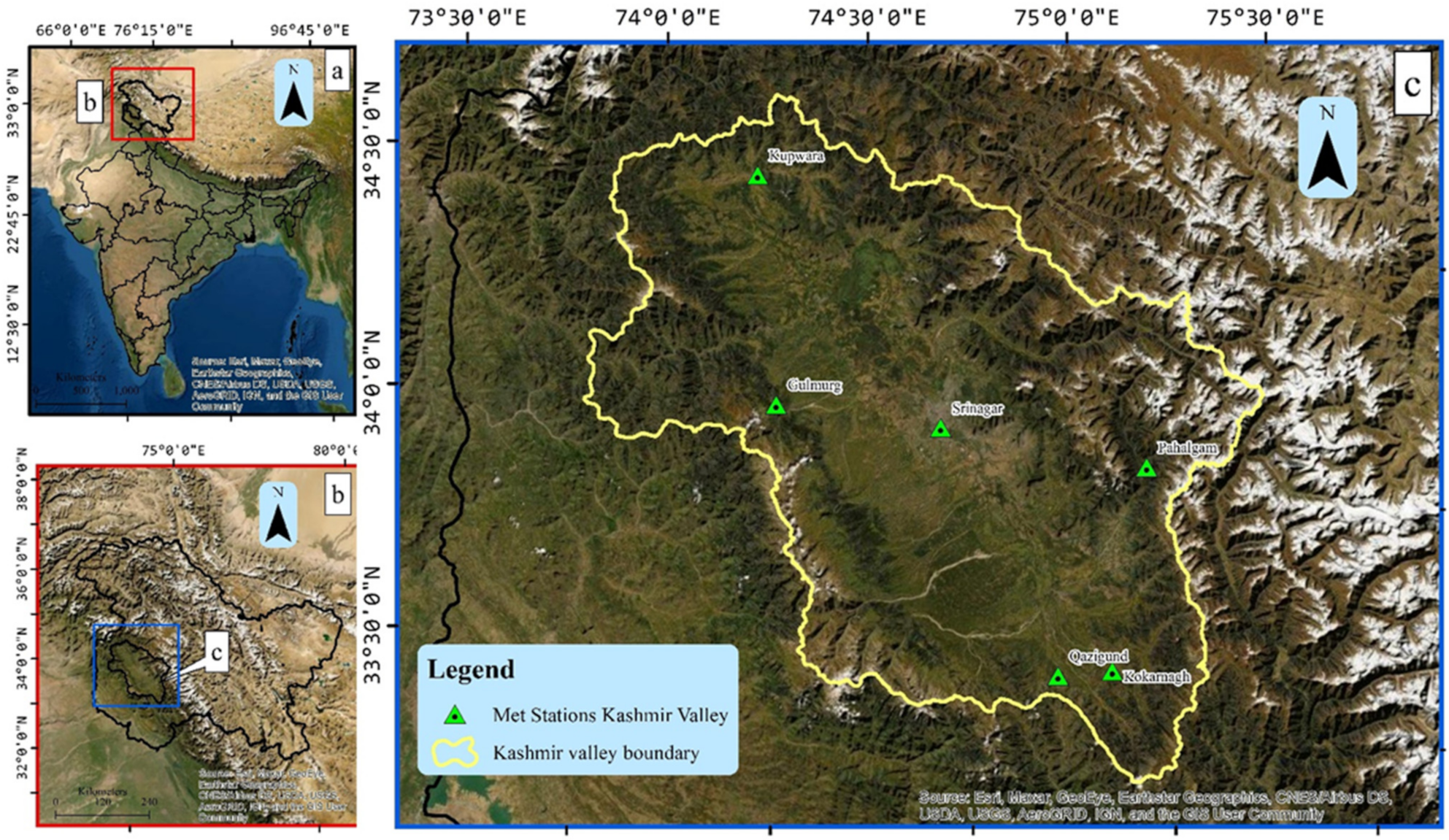
2.1. Study Area

Kashmir Valley on the south is bordered by the Pir Panjal range and by the western Himalayan peaks on the north side [42]. The Himalayan complex has a pervasive influence on the valley’s geographic entity. The total area of the region is about 15,948 km². The oval-bowl shaped valley extends from latitudes, 32°22′–34°43′ N and longitudes, 73°52′–75°42′ E with an elevation range of 1300–1800 masl as shown in Figure 1. It is traversed by the Jhelum river, one of the Indus basin tributary. The weather in the Kashmir valley keeps on fluctuating owing to elevational differences [30].

Summer monsoons originating in the Indian Ocean and Central Siberia’s winter air masses are separated by the mountain ranges of the valley that act as a barrier to them [29]. Westerly troughs moving during the winter at higher altitudes enter the west and northwest of the valley, while the greater Himalayas obstruct their influx. The climate is unpleasant above the tops of surrounding mountains due to micro-level variations but generally warm and temperate over the valley. With more than 105 glaciers, the Kashmir valley is an important watershed of the upper Indus basin (UIB) [43]. Based on mean temperature and precipitation, the Kashmir valley’s climate is characterized as sub-Mediterranean type with four seasons, spring (March–May), summer (June–August), autumn (September–November), and winter (December–February), [44]. The winters are usually cold and unpleasant, and summers are scorching, while spring is usually wet and autumn is dry. The valley’s annual temperature ranges from −10 to 35 ℃. Winter precipitation is coupled with western disturbances, dominates the rainfall pattern in the valley [45], while snowfall occurs primarily in the winter and early spring [46,47].

2.2. Datasets

The Himalayas (Greater), valley floor (Jhelum), and the Pir Panjal divide the Kashmir valley into three physiographic regions. Six well-distributed meteorological stations with varying mean sea levels, namely Gulmarg station (2740 m), Pahalgam station (2600 m), Kokarnag station (2000 m), Srinagar station (1600 m), Kupwara station (1670 m), and Qazigund station (1650 m), were chosen to represent the entire valley for analyzing the spatiotemporal variations in climatic variables (

Table 1. List of data ranges, basic geographic characteristics, and variables for those stations used in this study.

S.No.	Met Stations	Latitude	Longitude	Resolution	Time Period	Variables
1	Srinagar	34.05	74.80	Monthly	1980–2019	Tmax, Tmin, Precp
2	Gulmarg	34.06	74.39	Monthly	1980–2019	Tmax, Tmin, Precp
3	Kupwara	34.53	74.27	Monthly	1980–2019	Tmax, Tmin, Precp
4	Phalgham	34.02	75.33	Monthly	1980–2019	Tmax, Tmin, Precp
5	Qazigund	33.60	75.17	Monthly	1980–2019	Tmax, Tmin, Precp
6	Kukarnagh	33.59	75.30	Monthly	1980–2019	Tmax, Tmin, Precp

and Figure 1). These six stations’ topographic setting is characterized into two groups: (1) stations located on the plains (Qazigund, Kokarnag, Srinagar, and Kupwara) and (2) stations located in the mountainous areas (Pahalgam and Gulmarg) [32]. The data used were collected from the IMD-Srinagar and IMD-Pune centers for the period of 40 years (1980–2019) of six ground-based meteorological stations. This time series was deemed adequate for trend analysis to observe the fluctuations in different time scales at various climatic variables in the region. In order to understand climatic fluctuations over the region, inter and intra-annual trend analysis was carried out. The double-mass curve analysis method was utilized to cross-examine and check the data’s homogeneity and consistency, which might have occurred due to instrumentation error [48].

In prior studies on meteorological time series data, different statistical approaches (parametric and non-parametric) were used for determining whether the observed values of a hydro-meteorological time series are increasing, decreasing, or trendless. However, parametric methods with many restricted measures such as normal distribution and serially independent data are considered more powerful than non-parametric approaches, which is hardly true when it comes to meteorological time series data [49]. Non-parametric approaches, on the other hand, have been employed to identify trends in hydro-meteorological time series data since they don’t need data to be distributed normally; nonetheless, this is the necessity for data to be free of serial correlation. A pre-whitening method was used to remove the serial correlation prior to using the MK test on the meteorological time series data [50]. Using the pre-whitening method on time series data, on the other hand may compromise the uniqueness of the data and erase a trend component that is truly present [51,52]. As a result, [53] suggested ITA technique that does not require such preprocessing in addition to having broad applications.

The results of the ITA approach are compared with those of MK and Sen’s slope tests to assess the approach’s trustworthiness. The annual and seasonal precipitation and air temperature time series were analyzed using ITA method for six stations across the valley. The monthly data were averaged for temperature and precipitation to develop the seasonal and annual precipitation time series [49,54]. Further, the air temperature and precipitation time series trends were analyzed at 10 percent, 5 percent, and 1 percent levels of significance using the ITA, MK, and Sen’s slope approaches. A significance threshold of 10 percent level was used to establish a significant trend.

2.3. MK and Sen’s Slope Tests

The non-parametric MK test is one of the robust statistical trend method for hydro-meteorological time series to detect the monotonic trends because of outlier’s insensitivity and normal distribution [55,56,57].

The MK statistics, S is known as:

$$S={\displaystyle \sum _{k=1}^{n-1}{\displaystyle \sum _{j=k+1}^n\mathrm{sgn}(Y_j-Y_k)}}$$

(1)

$$\mathrm{sgn}(Y_j-Y_k)=\left\{\begin{array}{ccc}if(Y_j-Y_k)<0;& then& -1\\ if(Y_j-Y_k)=0;& then& 0\\ if(Y_j-Y_k)>0;& then& 1\end{array}\right\}$$

(2)

Here, Y_k and Y_j are successive data points of time-series with period k and j, n defines the no. of points, sgn represents the fn. taking the values of 1, 0, and −1; if >, Y_j = Y_k and Y_j < Y_k, respectively. +ve values of S define the upward trend, and −ve values of S denote a decreasing trend in the hydro-meteorological time series [58]. The size of the sample for which n > 10, the test has to be escorted through a normal distribution (σ² = 1) and average (µ = 0) with variance (Var) and probability (E) as presented below:

$$E\left[S\right]=0$$

(3)

$$Var(S)=\frac{n(n-1)(2n+5)-{\displaystyle {\sum }_{p=1}^q{t}_p(t_p-1)(2t_p+5)}}{18}$$

(4)

where q is the taut groups signifying observations having the common value, excluding unique rank numbers position, t_p defines the no. of data points of the pth group, symbol (∑) describes all the tied groups summation. Var(S) is the variance after manipulating from Equation (4), the test statistics standardized value (Z_MK) is evaluated by means of the eqn. below:

$$Z_{MK}=\left\{\begin{array}{ccc}\frac{S-1}{\sqrt{VAR(S)}},& if& S>0\\ 0,& if& S=0\\ \frac{S+1}{\sqrt{VAR(S)}},& if& S<0\end{array}\right.$$

(5)

Normal distribution with variance is followed by the regular Z_MK values follow a “1” and means “0,” and is employed for calculating the variational weight. It is employed for checking the null theory, H₀. If Z_MK is bigger than Z_α/2, consequently, the data series shows trends that are significant. Such a calculated estimation of Z_MK is matched with the two-tailed test table for normal distribution pertaining to α confidence level = 10%. However, for tests that is two-tailed, the null theory (H₀) is settled for zero (no) trend if the calculated estimation of Z_MK falls from—Z1-_α/2 through Z1-_α/2, and so, H₁ is excluded. In our study, the meteorological time series data trends are assessed for the levels of significance of 1%, 5%, and 10%.

The non-parametric Sen’s slope estimator test is used for assessing the trend’s weight in time series data [59,60]. The slope for n number of pairs of data-values is assessed by means of the equation given below.

$$b_i=\begin{array}{ccc}median& \left[\frac{Y_j-Y_k}{j-k}\right]& \forall \left(k<j\right)\end{array}$$

(6)

where Y_j and Y_k defines data points at time j and k. The n number of values that are median of bi actually depicts Sen’s slope of trend. The +ve values of bi denote an increasing trend, while −ve values reveal the downward trend. Here, n = odd number, consequently the slope of the trend using Sen’s method is calculated as:

$$Q_{med}=b_{\left[\left(n+1\right)/2\right]}$$

(7)

where, n = even number, now the trend slope using Sen’s method is estimated as:

$$Q_{med}=\frac{1}{2}\left(b_{\left[n/2\right]}+b_{\left[\left(n+2\right)/2\right]}\right)$$

(8)

Finally, a two-tailed test is used to verify Q_med at desired confidence interval, and the real trend magnitude of the slope can be assessed through a non-parametric test [61].

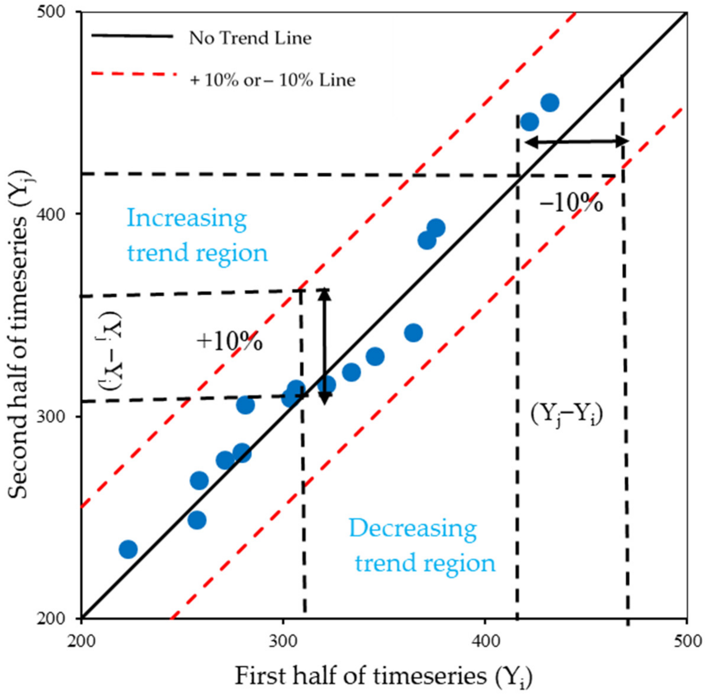
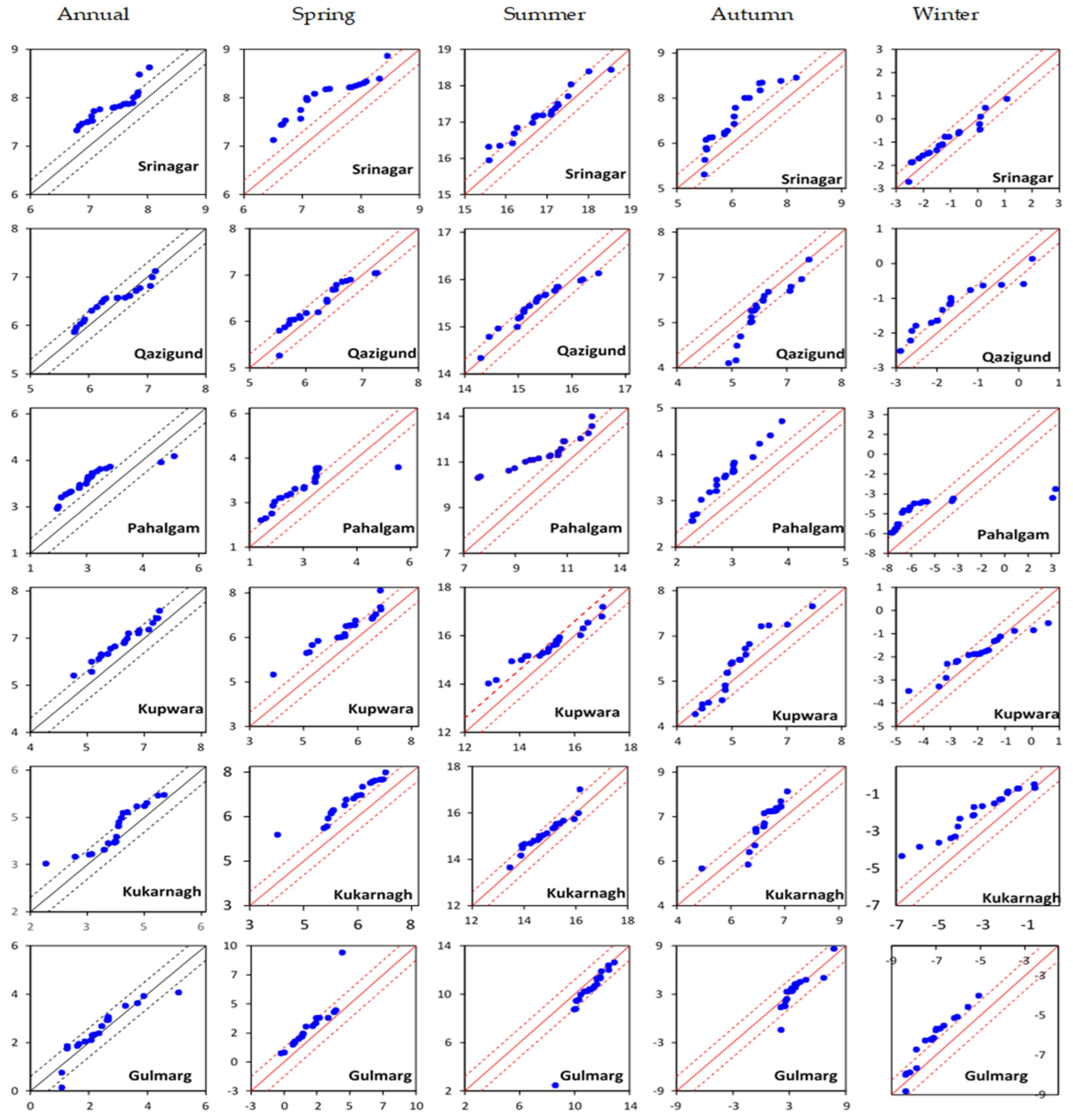
2.4. Innovative Trend Analysis (ITA) Method

Most studies have employed the innovative trend analysis (ITA) approach in conjunction with many further trend analysis approaches to find disparities in climatological, meteorological, and hydrological data time series around the world due to its advantages over other non-parametric approaches. The trustworthiness of ITA is proven, however, by matching its results to those with the MK test results. The initial stage in this strategy is to divide hydro-meteorological time series data into 2 equal halves and position each one in increasing order separately. The second stage involves, the first 1/2 of the sub-series (X_i; i = 1, 2… n/2) positioned at X-axis, with the second 1/2 (X_j; j = n/2 + 1, n/2 + 2… n) is positioned at Y-axis of cartesian coordinate system, as illustrated in Figure 2. Both the axes (vertical & horizontal) necessarily have the same range. A series of clusters can be used to describe the domain variance of each sub-series (subgroups). This type of graph provides a quick visual inspection of the nature of time-series trends. Each subgroup’s range can be resolute qualitatively or numerically. Data values on the scatter plot may be collected on the 45°-1:1 linear line. The hydro-meteorological time series has no trend. Otherwise, data values accumulating at the area of triangulation below or above the linear line specify an upward trend or a downward trend within the time series, respectively [53]. On computing the average difference between the X_j and X_i values at every point, the increasing or downward longitudinal trend in the time series can be evaluated. The horizontal and vertical distance from the linear line can be used to calculate this absolute difference. When comparing the amplitude of two subseries’ trends, however, these average disparities should be normalized. The first half of the time series is used to determine the trend change. As a result, the indicator of trend is derived by dividing the mean difference between the linear line and the time series’ first 1/2. On multiplying by ten the ITA trend indicator has represented the scale of the Sen’s slope estimator and MK test at a 10% significance level as shown in the equation below:

$$D=\frac{1}{n}{\displaystyle \sum _{i=1}^n\frac{10\left(Y_j-Y_i\right)}{\mu }}$$

(9)

Here, D denotes the indicator of trend, n the number for data points in each sub-series, Y_i and Y_j denote the 1st and 2nd sub-series data points, respectively µ denotes the first subseries average. However, the +ve or −ve values of D represent an increasing or decreasing trend, respectively. If the value of observational data in the original time-series are found odd, at that time the initial results might be omitted earlier when dividing it into two equal halves so as to make the recent records are fully utilized.

3. Results

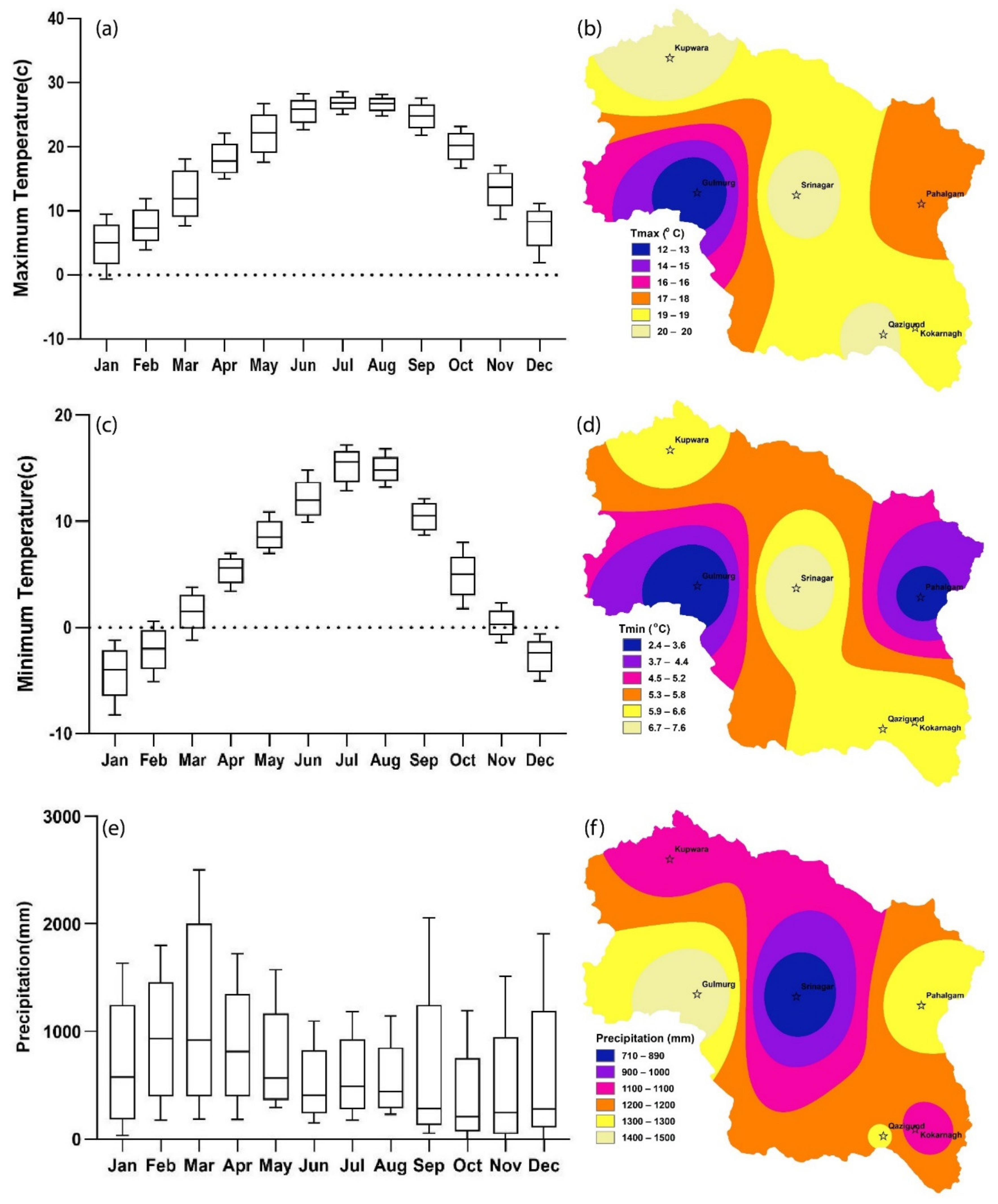
3.1. Spatio-Temporal Variations of T_max, T_min and Precipitation for Kashmir Valley Stations

Seasonal T_max, T_min, and precipitation time series at six stations were investigated for spatiotemporal changes in Kashmir valley are presented in Figure 3. The average observed monthly T_max, T_min, and precipitation at six dissimilar stations was combined to signify the overall temporal distribution of T_max, T_min, and precipitation throughout the Kashmir valley. Due to the northern side of the Himalayas, the valley (Kashmir) is influenced by several climate regimes such as westerly disturbances, monsoonal effects, and orographic fluctuations, making it a complicated region. The annual T_max, T_min, mean temperature and precipitation in the valley stations were approximately 20 ℃, 7.6 ℃, 13.8 ℃, and 723.8 mm for Srinagar, 19.3 ℃, 6.4 ℃, 12.8 ℃ and 1212.7 mm for Qazigund, 16.6 ℃, 3.1 ℃, 9.8 ℃ and 1288.9 mm for Pahalgam, 20.1 ℃, 6.3 ℃, 13.2 ℃ and 1081.2 mm for Kupwara 18.1 ℃, 4.1 ℃, 11.1 ℃, and 1080.2 mm for Kukarnagh 11.7 ℃, 2.4 ℃, 7.0 ℃ and 1485.1 mm for Gulmarg station for the period of forty years (1980–2019) as shown in

Table 2. T_max, T_min, and Mean temperature and precipitation mean in Kashmir valley stations over a multi-year period.

Stations Name	Seasons	Tmax	Tmin	Mean-Temperature	Precipitation
		1980–2019	1980–2019	1980–2019	1980–2019
Srinagar	Annual	20.0	7.6	13.8	723.8
	Spring	20.1	7.7	13.9	281.0
	Summer	29.3	17.0	23.2	173.0
	Autumn	21.7	6.7	14.2	93.0
	Winter	8.8	−1.1	3.9	172.5
Qazigund	Annual	19.3	6.4	12.8	1212.7
	Spring	19.4	6.3	12.8	135.9
	Summer	27.7	15.3	21.5	82.5
	Autumn	21.4	5.8	13.6	43.8
	Winter	8.7	−1.9	3.4	129.1
Pahalgam	Annual	16.6	3.1	9.8	1288.9
	Spring	16.6	2.9	9.7	463.9
	Summer	25.0	11.2	18.1	300.1
	Autumn	18.6	3.2	10.9	181.6
	Winter	6.1	−4.9	0.6	332.6
Kupwara	Annual	20.1	6.3	13.2	1081.2
	Spring	19.8	6.2	13.0	442.4
	Summer	29.5	15.3	22.4	207.7
	Autumn	22.5	5.6	14.1	138.9
	Winter	8.6	−1.9	3.3	281.4
Kukarnagh	Annual	18.1	4.1	11.1	1080.2
	Spring	18.4	6.4	12.4	394.3
	Summer	27.0	14.9	21.0	259.3
	Autumn	19.9	6.8	13.3	151.2
	Winter	7.1	−2.1	2.5	267.7
Gulmarg	Annual	11.7	2.4	7.0	1485.1
	Spring	10.8	1.9	6.4	176.3
	Summer	20.0	10.7	15.3	104.3
	Autumn	13.2	3.1	8.2	63.3
	Winter	2.6	−6.0	−1.7	439.6

. Furthermore, the precipitation was mainly concentrated in the spring and winter in all stations across the valley, with summer precipitation contributing a good portion also.

The mean monthly T_max, T_min and precipitation over the Kashmir valley are presented in Table 2. The annual precipitation over the Kashmir valley was governed by two climatic systems, the Indian summer monsoons (ISM) and the Western Disturbances. Over three-quarters of precipitation (71.54%) account for Western Disturbances from October to May, with the peak monthly precipitation occurring in Mar through May of the spring season. However, the residual 28.46% of rainfall falls between June and September, with a cluster of highest monthly precipitation in September Figure 3e,f, which is attributed to the Indian Summer Monsoon (ISM). Kashmir valley is influenced by mid-latitude westerlies considerably and is captured by the northern part represented by the two IMD stations, Gulmarg and Kupwara, while the south side of the valley was influenced by ISM and was captured by three IMD stations (Kukarnagh and Pahalgam and Qazigund) [30,62].

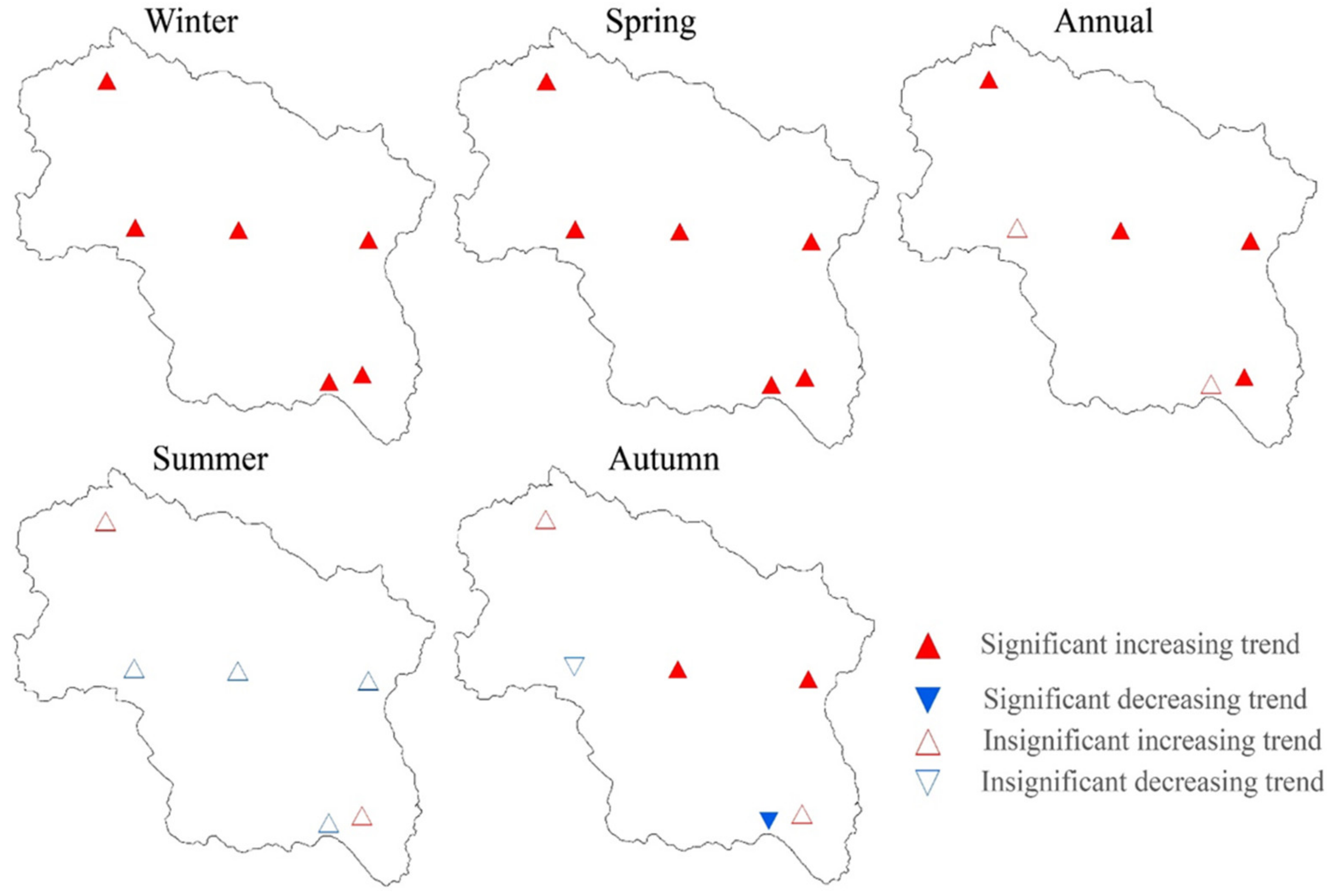
3.2. Annual and Seasonal T_max Variations over Time

The annual and seasonal T_max over the Kashmir valley stations are examined using the MK test and their results are summarized in

Table 3. Summarized results for the seasonal T_max time series using ITA method statistic D, MK test statistic Z and Sen’s slope estimator β.

S.No.	Station Name	Annual			Spring			Summer			Autumn			Winter
		ITA	Zmk	Sen Slope (β)	ITA	Zmk	Sen Slope (β)	ITA	Zmk	Sen Slope (β)	ITA	Zmk	Sen Slope (β)	ITA	Zmk	Sen Slope (β)
1	Srinagar	0.57	2.92 **	0.04	0.88	2.23 *	0.05	0.04	−0.20	0.00	0.37	2.34 *	0.04	2.17	2.81 **	0.06
2	Qazigund	0.22	1.13	0.01	0.70	2.16 *	0.04	−0.06	−0.62	0.00	−0.13	−2.11 *	−0.03	1.32	1.85 +	0.04
3	Pahalgam	0.56	2.80 **	0.04	0.94	2.21 *	0.05	−0.13	−1.00	−0.01	0.36	1.68 +	0.03	3.45	3.93 ***	0.08
4	Kupwara	0.58	3.18 **	0.04	1.06	2.62 **	0.07	0.20	1.06	0.02	0.15	1.06	0.02	2.04	3.30 ***	0.06
5	Kukarnagh	0.60	2.57 *	0.04	0.96	2.20 *	0.06	0.07	1.25	0.01	0.27	0.73	0.01	2.75	2.57 *	0.06
6	Gulmarg	0.25	0.85	0.01	1.55	1.71 +	0.05	−0.20	−0.83	−0.02	−0.50	−0.52	−0.01	2.44	1.78 +	0.04

*** if trend at α = 0.001 level of significance. ** if trend at α = 0.01 level of significance. * if trend at α = 0.05 level of significance. + if trend at α = 0.1 level of significance. If the cell is blank, the significance level is greater than 0.1.

. Annual T_max showed significant increasing trends at Srinagar, Pahalgam, Kupwara, and Kukarnagh stations (α = 0.01, α = 0.05) whereas Qazigund and Gulmarg stations also exhibited an increasing trend but statistically insignificant trends. Spring T_max showed significantly increasing trends at Kupwara (α = 0.01), Srinagar, Qazigund, Pahalgam, and Kukarnagh stations (α = 0.05) and Gulmarg (α = 0.1). The summer T_max showed a decreasing trend at Srinagar, Qazigund, Pahalgam, and Gulmarg stations, while Kupwara and Kukarnagh stations exhibited increasing trends. Autumn T_max showed a significantly increasing trend for Srinagar and Pahalgam stations (α = 0.05, α = 0.1) and a significantly decreasing trend for the Qazigund station (α = 0.05). Winter T_max indicates a significantly increasing trend for all the stations, Srinagar (α = 0.01) Pahalgam and Kupwara (α = 0.001) Kukarnagh (α = 0.05) Qazigund and Gulmarg station (α = 0.1) as presented in Figure 4.

The annual and seasonal trends of T_max based on Innovative Trend Analysis (ITA) over the Kashmir valley stations are summed-up in Table 3 and Figure 5. The trends for the annual T_max showed positive values of ITA statistic D dominated statistics, showing mostly significant increasing trends. At Srinagar, Kupwara, Kukarnagh, Pahalgam and Qazigund stations, significantly increasing and decreasing trends for the annual T_max data points were observed falling above 10% range from the 1:1 line, In comparison, Gulmarg station’s majority of temperature data points fall in +10% range showing increasing trend with few points fall in −10% range from the 1:1 line during the period of forty years (1980–2019). The trends for T_max for the spring season statistics exhibited by significant (positive) values of ITA D, which is evidence of an increasing trend, are summarized in Table 3.

Srinagar, Qazigund, Pahalgam, Kupwara, and Kukarnagh stations showed increasing and decreasing trends for T_max data points, falling above 10% range from 1:1 line depicting a significantly positive trend. In comparison, Gulmarg station exhibited the increasing and decreasing trend for T_max data points which falls on +10% range from the 1:1 line. Summer T_max trends exhibited positive values of ITA statistic D increasing trend for three stations (Srinagar, Kupwara, and Kukarnagh) and negative values for three stations (Qazigund, Pahalgam, and Gulmarg). The combination of T_max data points falls within the range of 10% from the 1:1 line, which exhibits the decreasing trend for Srinagar and Qazigund stations. In contrast, Kupwara Pahalgam stations showed a decreasing trend for T_max data points falling in the 10% range. The results suggest that T_max trends for the autumn season showed four stations with significant positive values (Srinagar, Pahalgam, Kupwara, and Kukarnagh) and two stations with significant negative values (Qazigund and Gulmarg). In autumn, most T_max data points for Srinagar, Pahalgam, Kupwara, and Kukarnagh stations fall on the +10% range from the 1:1 line with an increasing trend. In comparison, Qazigund and Gulmarg showed T_max data points falling over the −10% range with an insignificant decreasing trend. The T_max for the winter season showed that all the station’s ITA statistics for D exhibit positive values with a significant increasing trend. Moreover, an increasing and decreasing trends combination for T_max data points that fall above the 10% range from the 1:1 line exhibit a significantly positive trend for all the stations except Gulmarg station. The latter exhibited that the T_max data points falling on the +10% range of 1:1 linear line with an upward trend.

Results depict an overall increase in the annual temperature is largely attributed to a mean T_max. It is clear for Figure 5 that it is reasonable to conclude that the climate in the Kashmir valley is fluctuating towards a system subjugated by high temperatures; as a result, the spring and winter seasons are changing in their durations.

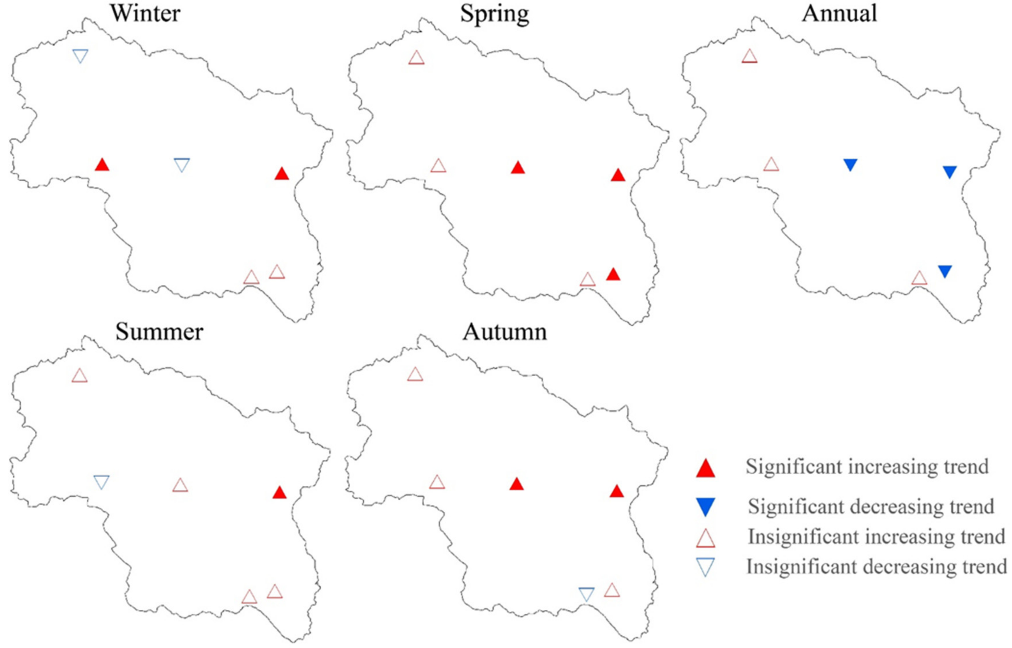
3.3. Annual and Seasonal T_min Variations

Significant increasing trend based on Mann Kendall (MK) were noticed at Srinagar, Pahalgam (α = 0.01), Qazigund (α = 0.001) and Kupwara (α = 0.05) stations whereas Kukarnagh and Gulmarg stations displayed an increasing but insignificant trend in the annual T_min as summarized in

Table 4. Summarized results for the seasonal T_min time series using ITA method statistic D, MK test statistic Z and Sen’s slope estimator β.

S.No.	Station Name	Annual			Spring			Summer			Autumn			Winter
		ITA	Zmk	Sen Slope (β)	ITA	Zmk	Sen Slope (β)	ITA	Zmk	Sen Slope (β)	ITA	Zmk	Sen Slope (β)	ITA	Zmk	Sen Slope (β)
1	Srinagar	0.58	2.83 **	0.02	0.80	2.50 *	0.02	0.20	1.43	0.01	0.96	3.55 ***	0.04	−1.47	−0.15	0.00
2	Qazigund	0.14	0.85 ***	0.00	0.21	0.43	0.00	0.11	0.94	0.01	−0.59	−0.10	0.00	−1.61	0.62	0.01
3	Pahalgam	2.72	3.66 **	0.04	1.62	2.14 *	0.03	1.27	2.91 **	0.05	2.01	3.45 ***	0.03	−1.23	2.18 *	0.04
4	Kupwara	0.62	1.27	0.04	1.10	1.62	0.07	0.31	0.97	0.02	0.53	1.06	0.02	−0.63	−0.48	0.06
5	Kukarnagh	0.77	2.27	0.02	1.41	2.18 *	0.03	0.21	0.66	0.01	0.60	1.29	0.01	−4.44	1.20	0.03
6	Gulmarg	0.40	0.97	0.01	7.00	1.32	0.03	−0.81	−0.90	−0.02	−2.14	1.06	0.02	−1.45	2.62 **	0.05

*** if trend at α = 0.001 level of significance. ** if trend at α = 0.01 level of significance. * if trend at α = 0.05 level of significance. If the cell is blank, the significance level is greater than 0.1.

. Spring T_min exhibited a significantly increasing trend for Kupwara, Srinagar, Pahalgam, and Kukarnagh stations (α = 0.05, α = 0.01) while Qazigund and Gulmarg exhibited an increasing but insignificant trend. The summer T_min indicates a significantly increasing trend for Pahalgam Srinagar, Qazigund, Kupwara, and Kukarnagh (α = 0.01), whereas for Gulmarg exhibited decreasing but an insignificant trend. Autumn T_min exhibited a significantly increasing trend for Srinagar, Pahalgam, Kupwara, Kukarnagh, and Gulmarg (α = 0.001), with Qazigund showing decreasing but insignificant trend. Winter T_min exhibits a significant increasing trend for Kupwara (α = 0.001), Gulmarg (α = 0.01), and Pahalgam (α = 0.05) while Qazigund and Kukarnagh exhibit an increasing trend with Srinagar showing a significantly decreasing trend as presented in Figure 6.

Annual (annual) and seasonal T_min trends based on Innovative Trend Analysis for Kashmir valley are summed up in Table 4 and Figure 7. The trends for annual T_min for all the stations showed that the statistics for ITA D were dominated by positive values evident of increasing trend. The combination of increasing and decreasing trends for T_min data points falls above the 10% range for Srinagar and Pahalgam stations. However, Qazigund, Kupwara, Kukarnagh, and Gulmarg’s T_min data points fall on a +10% range from the 1:1 line. The trends for spring T_min for all the stations showed that the statistics were significantly positive dominated. Moreover, the combination of upward and downward trends for T_min data points falls on the +10% range for Qazigund and Gulmarg stations. In contrast, Srinagar, Pahalgam, Kupwara, and Kukarnagh have T_min data points that mostly fall >10% range from the 1:1 line. The trends for summer T_min for all the stations showed that the statistics for ITA D were positively dominated, which exhibits the insignificant increasing trend except for the Gulmarg station, which exhibits a negative trend. However, Pahalgam station exhibits a significant increasing trend, as summarized in Table 4. The combination of increasing and decreasing trends for T_min data points falls on +10% range for Srinagar, Qazigund, Kupwara, and Kukarnagh stations whereas, Gulmarg station is at −10% with Pahalgam station as exception data points falls >10% range from 1:1 line. The trends for autumn T_min for Srinagar, Pahalgam, Kupwara, and Kukarnagh showed positive values, with significantly increasing trends for Srinagar and Pahalgam. Further, the combination of increasing and decreasing T_min data points for Qazigund, Kupwara, Kukarnagh, and Gulmarg stations falls within the 10% range.

In comparison, Srinagar and Pahalgam station’s T_min data points fall above the 10% range from the 1:1 line. The trends for winter T_min for all the stations showed negative values for ITA of D-dominated statistics. Most of them were significantly decreasing trends, which are summarized in Table 4. The combination of increasing and decreasing for T_min data points for Srinagar, Qazigund, and Kupwara stations falls in the +10% range, while Pahalgam, Kukarnagh, and Gulmarg stations T_min data points fall above the 10% range from 1:1 line. The overall results suggest that T_min is in comparison with the T_max. It may be noted that the spring and winter seasons are warming in this region than the autumn and summer seasons. This anomaly contributes towards a reduction in the snow depth/cover and shrinking of glaciers.

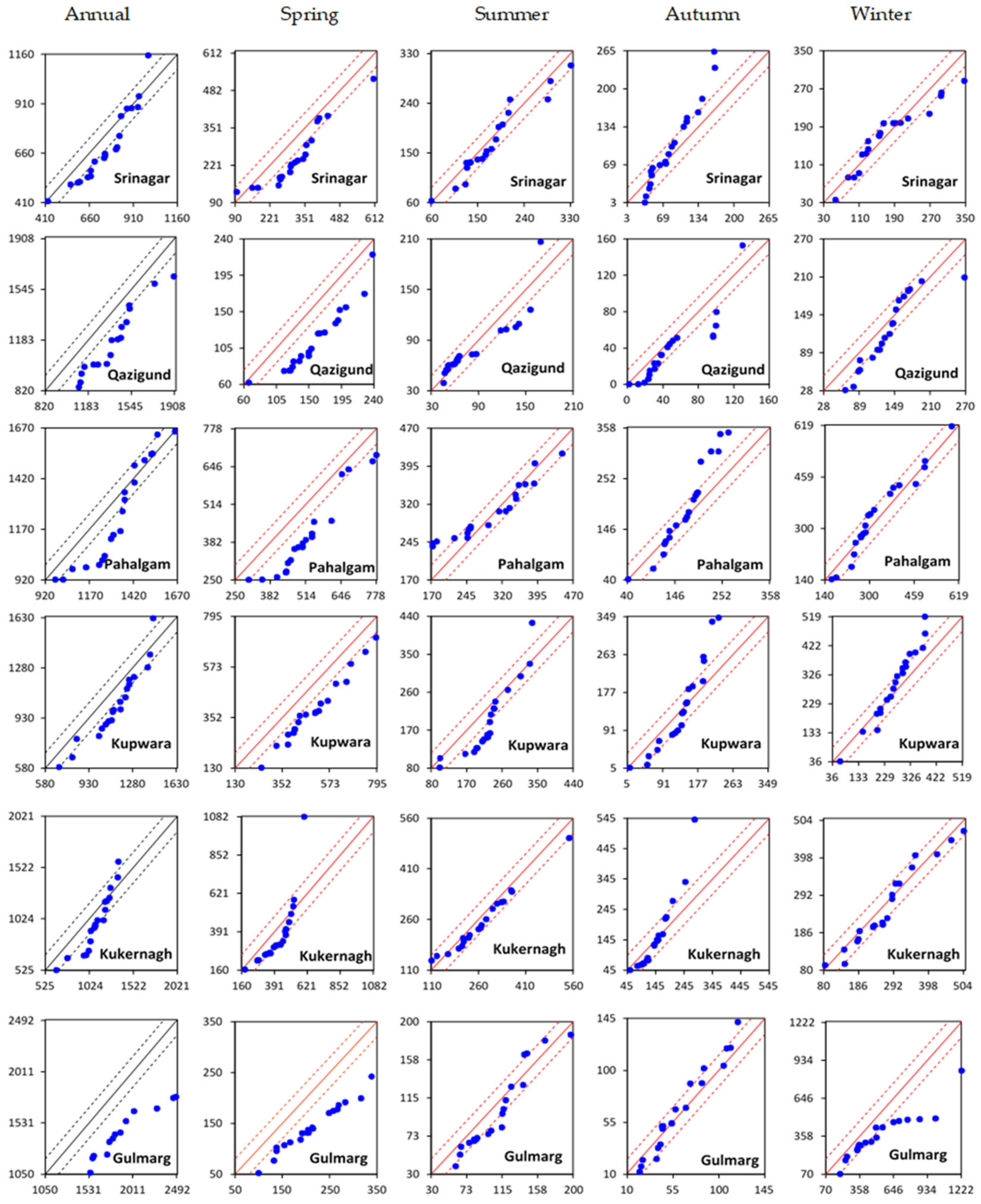
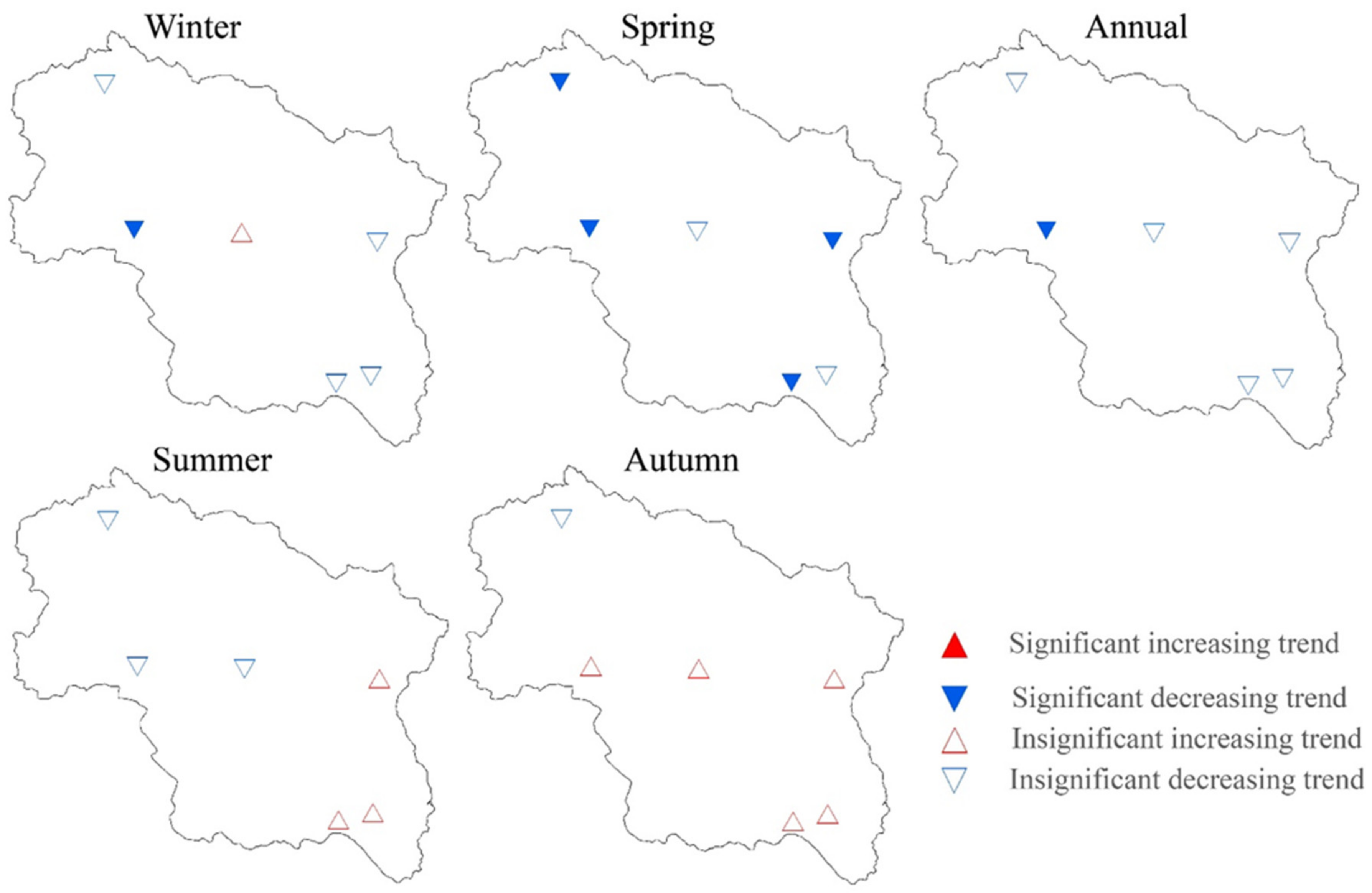
3.4. Annual and Seasonal Precipitation Variations over Time

Table 5. Summarized results for the seasonal precipitation time series using ITA method statistic D, MK test statistic Z and Sen’s slope estimator β.

S.No.	Station Name	Annual			Spring			Summer			Autumn			Winter
		ITA	Zmk	Sen Slope (β)	ITA	Zmk	Sen Slope (β)	ITA	Zmk	Sen Slope (β)	ITA	Zmk	Sen Slope (β)	ITA	Zmk	Sen Slope (β)
1	Srinagar	−0.78	−0.36	−1.08	−2.09	−1.27	−2.02	−0.48	−0.34	−0.22	1.88	0.15	0.15	−0.30	0.08	0.09
2	Qazigund	−1.64	−1.18	−5.59	−2.72	−2.53 *	−5.31	−0.46	0.66	0.60	−2.55	0.10	0.18	−1.14	−1.55	−2.96
3	Pahalgam	−0.61	−0.42	−1.29	−2.20	−2.28 *	−4.73	0.26	0.77	0.70	1.27	1.26	1.65	0.23	−0.26	−0.60
4	Kupwara	−1.03	−1.57	−5.57	−2.28	−1.85 +	−3.71	−1.45	−1.35	−1.28	0.61	−0.17	−0.19	1.03	−0.17	−0.32
5	Kukarnagh	−0.58	−0.20	−0.68	−0.90	−1.50	−2.99	−0.68	0.70	0.77	0.69	0.27	0.31	−0.44	−0.61	−1.09
6	Gulmarg	−2.42	−2.34 *	−12.30	−3.36	−2.64 **	−2.37	−0.90	−0.69	−0.40	0.51	0.45	0.27	−3.10	−2.41 *	−5.69

** if trend at α = 0.01 level of significance. * if trend at α = 0.05 level of significance. + if trend at α = 0.1 level of significance. If the cell is blank, the significance level is greater than 0.1.

represents the annual (annual) and seasonal trends using Mann Kendall (MK) test over Kashmir valley. Annual precipitation exhibited decreasing trend but was significant for the Gulmarg station (α = 0.05), while the rest of the stations exhibited insignificant decreasing trends. Spring precipitation indicated a significantly decreasing trend for Gulmarg (α = 0.01), Qazigund, Pahalgam (α = 0.05), and Kupwara (α = 0.1), while Srinagar and Kukarnagh stations exhibited decreasing insignificant trend. Summer precipitation for Srinagar, Kupwara, and Gulmarg stations displayed a downward trend while Qazigund, Pahalgam, and Kukarnagh stations exhibited an increasing significant trendMeanwhile, autumn precipitation showed an increasing trend for all stations except Kupwara, which exhibited an insignificant decreasing trend. Winter precipitation exhibited a significantly decreasing trend for Gulmarg (α = 0.05) while Qazigund, Pahalgam, Kupwara, and Kukarnagh exhibited decreasing trends except for Srinagar station, which showed an increasing but significant trend as presented in Figure 8.

The annual (annual) and seasonal precipitation trends results based on Innovative Trend Analysis (ITA) for Kashmir valley stations are presented in Figure 9 and Table 5. The annual precipitation trends for all the stations showed negative values for ITA of D dominated statistics, with Qazigund, Kupwara, and Gulmarg stations showing significantly decreasing trends, as summarized in Table 5. The grouping of increasing/decreasing trends for precipitation data points falls <10% range for Qazigund and Gulmarg stations. However, Srinagar, Kupwara, and Kukarnagh showed that the precipitation data points fall in the −10% range, with Pahalgam station showing a majority of data points below and some on +10% range from the 1:1 line. The trends for spring precipitation for all the stations showed that statistics for ITA of D values were negatively dominated, while Srinagar, Qazigund, Pahalgam, Kupwara, and Gulmarg stations were showing significant decreasing trends as summarized in Table 5 and presented in Figure 9, while Kukarnagh station showed an increasing trend but not significant. The increasing and decreasing trends combination for precipitation data points falls in <10% range for Srinagar, Qazigund, Pahalgam, Kupwara, and Gulmarg stations, with Kukarnagh station majority of data points −10% and some points fall in +10% range from the 1:1 line. The trends for summer precipitation for all the stations showed that negative values dominated statistics (decreasing trend), but all insignificant, as summarized in Table 5. The increasing and decreasing trends combination for precipitation data points falls in −10% range for Srinagar, Qazigund, Pahalgam, Kukarnagh, and Gulmarg stations with Kupwara station, showing that majority of precipitation data points ranges below from the 1:1 line and some are present on no trend line. The trends for autumn precipitation for all the stations showed that statistics of ITA of D were positively dominated, with Qazigund station as an exception showing negative values (decreasing) trend but insignificant. The increasing and decreasing trends combination for data points precipitation falls between 10% range on the 1:1 line for all observatories. The trends for the winter precipitation of all stations showed negative values of ITA for D dominated statistics with Pahalgam and Kupwara as exceptions showing positive (increasing trend), but all insignificant except for Gulmarg station, which is showing significant trend as summarized in Table 5. The increasing and decreasing trends combination for data points of precipitation falling between the 10% range for all stations except Gulmarg station, showing a majority of precipitation data points below (<) and some points are at −10% range from the 1:1 line. The results for overall precipitation suggest drought conditions for Kashmir valley; however, decreases in spring and winter precipitation are in agreement with the temperature suggesting seasonal inconsistency and strong inter-station, which results in a visible shift in precipitation pattern.

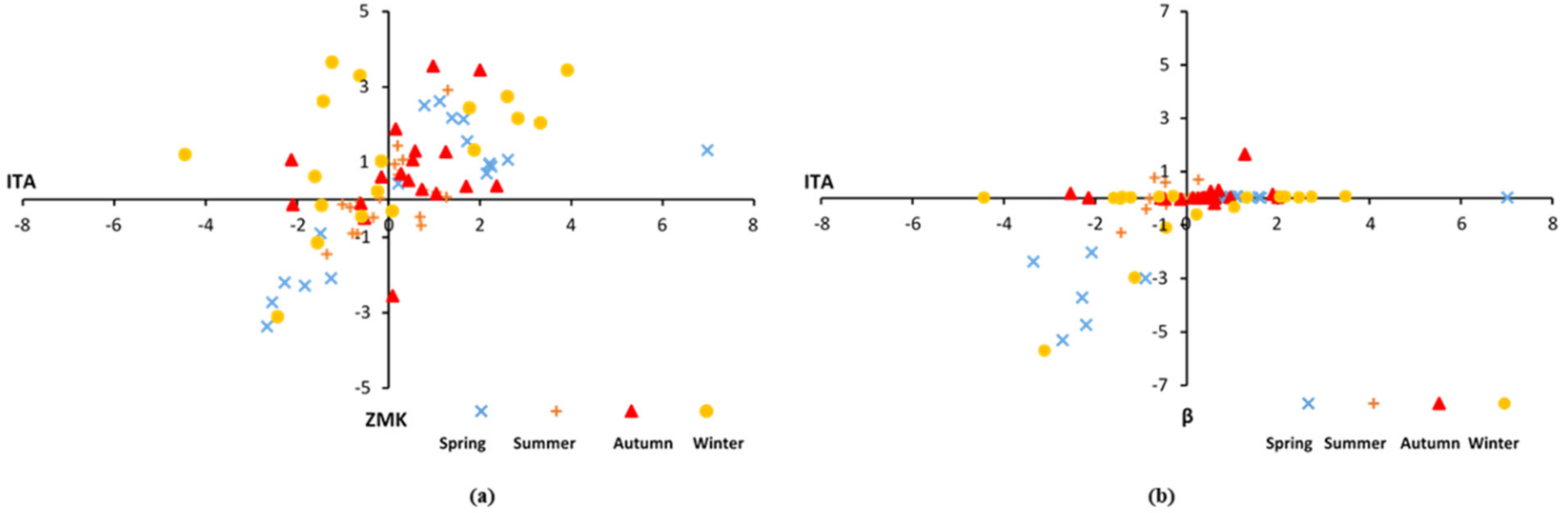
3.5. Comparison of ITA, MK, and Sen Slope Estimation Approach Results

On 40 years data annual and seasonal time series, MK and Sen’s slope estimator tests have been used for assessing the reliability of the ITA method. Except for the Gulmarg station, winter season of T_min and precipitation, nine (09) time series on a seasonal time-scale prove significant trends at dissimilar observatories that are sign-steady under the above-mentioned approaches. In order to match the ITA results for all significant and insignificant trends, scatter plots were generated in between the Zmk of the MK with statistic D of the ITA technique and Sen’s slope estimator with statistic D of the ITA method as depicted in Figure 10a,b. The results demonstrate 80% widely held of the scatter points fall in between the 1st and 3rd quadrants, indicating all these methods are in general agreement. The other 20% of the points fall in between the 2nd and 3rd quadrants, with same sign fluctuation; nevertheless, the trends are insignificant, and their S, i.e., the scale of Sen’s slope is minimal. The Figure 10a,b also showed a high agreement between the ITA statistic D and the MK statistic Zmk and Sen’s slope estimator. As a result of this comparison, it is evident that ITA results are consistent across all trend detection approaches, indicating that it is a reliable and successful tool. The reason for this is its ability to assess meteorological and hydrological data patterns from graphical representations at low to high values. When compared to the MK test, which has various limitations such as seasonal cycle, normality of distribution, serially independent data, and time-series length, the ITA technique has universal applicability [38,49,53].

4. Discussion

The observed annual and seasonal T_min and T_max increase for six observational stations in the valley (Kashmir) has profound implications on the various land system and socio-economic processes operating in the region. These findings have substantiated the results of many previous studies on trend analysis for hydro-meteorological data from the Kashmir region. According to Kumar and Jain [42], T_max in the region (Kashmir) showed a significant increase (+0.04 to +0.05 °C/year) and T_min in the region (Jammu) (+0.030 to + 0.080 °C/year) had been detected when analyzed over the period 1980–2012. According to Singh et al. [63], Western Himalayas showed an increase in air temperatures, which are in line with the observed temperature trend for the Northwest Himalayas and the present study. [30] analyzed station-wise spatiotemporal variation of observed temperature in the Kashmir valley and found that T_max and T_min in the Valley showed an increase by 0.0350 °C and 0.0220 °C, respectively.

Shafiq, et al. [29] concluded that minimum temperatures in various topographic zones of the Kashmir valley increased at a relatively consistent rate of around 0.020 °C/year, with the peak rate of increase in the mountains (0.020 °C/year). Further, Zaz et al. [32], found that the annual mean temperature has increased by 0.8 degrees Celsius over 37 years (from 1980 to 2016), with T_max (0.97 °C) increasing faster than T_min (0.76 °C). The study also found that the Pahalgam (1.13 °C) and Gulmarg (1.04 °C) being at high altitudes have significantly increasing trends in temperature consistent with the results of the present study. This changing temperature pattern shall have serious environmental consequences, affecting food security and ecological sustainability in the region and water availability and other natural resources. Moreover, in all observational stations in the valley, the annual and seasonal precipitation patterns were found to have downward trends, consistent with the results of the previous studies. Zaz, et al. [32] studied the long and short-term precipitation patterns using LR, MK, Student’s t-tests, and cumulative deviation; however, the results from the study showed that spring precipitation is decreasing. Shafiq, et al. [29] examined the annual and season-wise precipitation in Kashmir Valley from 1980 to 2016 and found a −5.1 mm/year decline in annual precipitation. The long-term upward trend results for precipitation at Pahalgam and Gulmarg stations for two seasons (spring, summer), which are also compatible with the [32]. It had been observed that the northern stations of the Kashmir valley (Jhelum basin) recommend a moderately stronger monsoonal influence; meanwhile, two stations within the Kashmir valley (Jhelum basin) revealed a considerable increase in precipitation.

An obvious shift in precipitation regime can be seen from the north to the south of the basin, consistent with earlier research findings in this region which can be linked to the Western disturbances’ movements (WD). The seasonal precipitation in the region is controlled by large-scale circulations from western disturbances (WDs), and it affects the supply and inventory of water resources of the Kashmir valley (Jhelum basin) [64]. It is hence concluded that, in winter, precipitation gets increased, but in spring, it decreases, and this phenomenon linked to specific variations in the WD precipitation trends. This observed winter precipitation increase is inconsistent with observations and future projections of the incursions of western disturbances, combined with the drying of the spring season in the region. This also designates a less erratic future WD regime [32]. However, the beginning of snowmelt from the Jhelum basin is expected to change as the changes in the western disturbances become more common in the future, as projected by the climate models. Understanding the Kashmir valley’s climatic variability is crucial for improved management and use of the valley’s available water resources where the population is dependent on agriculture activities. As the Himalayan hydrology is controlled by snow and glaciers, the changing climate of the region is bound to have drastic impacts on its water resources. Climate change impacts are evident in the Kashmir Himalayas. Natural calamities such as landslides and floods posing a significant threat to the people and infrastructure of this region which are climate change consequences [65,66]. Due to increased climatic variability associated with the ongoing changing climate, the region has recently witnessed one of the worst flooding disasters of the century [32,67]. Moreover, changing precipitation patterns have already impacted the recharge of groundwater, water supply in the streams during lean periods, and agriculture. The increase in the trends of T_max and T_min in the valley, as observed in the present study, has led to the early onset of spring and snowmelt, thus affecting the region’s ecological setup. Moreover, as observed in the present study, decreasing trends in precipitation affect the water supply and management scenarios.

Hence assessing the trends in hydro-meteorological parameters such as T_max, T_min and Precipitation have helped to understand the variability associated with the changing climate in the fragile Kashmir valley in North-Western Himalayas [68]. It is because of the variability of trends at different stations, further extensive research on the climate of this region at the micro-level are needed. In order to check how climate may get changed, trend analysis is used to assess the hydro-metrological data, which may impact river discharge in the Kashmir Himalayas. However, the trend analysis will help us to know how river discharge will behave under projected climate scenarios for kashmir valley under different models like BCC-CSM2-MR, CNRM-CM6-1 and IPSL-CM6A-LR.

5. Conclusions

The present study addressed the climatic variability assessment for the Jhelum basin (Kashmir valley) using different statistical methods. The investigation of the annual and seasonal variations of the temperature and precipitation using the MK, Sen’s slope estimator, and ITA approaches revealed some interesting findings related to the changing climatic scenario in the Kashmir valley. The rising temperature in two seasons (spring and winter) was credited for this major warming trend. T_max was observed to be significantly increasing at spring and winter seasons as well as annually, in almost all the stations except the Gulmarg, which exhibited an increasing but non-significant trend. The mean annual T_min followed the same significant trends as T_max, barring Kukarnagh and Gulmarg stations which exhibited non-significant increasing trends. T_min in the spring season also shows a significant positive trend for all stations except Qazigund and Gulmarg stations across the 1980–2019 time period. This rise in temperature across the valley, coupled with a considerable surge in spring and winter temperatures, reveals that less snowfall in the winter season results in decreased snow cover/depth. However, even at a small increase in temperature, a good amount of snowmelt is happening on the glaciers, clearing the way for early springs. Furthermore, annual precipitation showed decreasing trends for all the stations across the Kashmir valley. A significant decreasing trend in precipitation was detected for Qazigund, Pahalgam, Kupwara stations for the spring season, whereas for Gulmarg station, spring and winter seasons exhibited significantly decreasing trends since 1980–2019. This changing temperature and precipitation patterns in the region might have catastrophic implications for agriculture, hydropower, and drinking water supplies, affecting the region’s food security and ecological sustainability.

However, understanding the climatic variability has various intrinsic uncertainties, which may arise from the secondary source data and area characteristics, particularly in mountainous in the Himalayan mountainous regions like Kashmir valley. Unavailability of the long-term time series data for air temperature and precipitation hinders the more accurate assessment of the region’s climate variability, owing to only six meteorological stations representing 15,500 km² area. However, the major findings from this research confirm well with the large-scale land system changes taking place in the form of increased melting rates of snow and glacier resources in the valley.

References

1. Rahmat, A.; Zaki, M.K.; Effendi, I.; Mutolib, A.; Yanfika, H.; Listiana, I. Effect of global climate change on air temperature and precipitation in six cities in Gifu Prefecture, Japan. J. Phys. Conf. Ser. 2019, 1155, 012070. [Google Scholar] [CrossRef]
2. Arora, N.K.; Fatima, T.; Mishra, I.; Verma, M.; Mishra, J.; Mishra, V. Environmental sustainability: Challenges and viable solutions. Environ. Sustain. 2018, 1, 309–340. [Google Scholar] [CrossRef]
3. Aamir, M.; Rai, K.K.; Dubey, M.K.; Zehra, A.; Tripathi, Y.N.; Divyanshu, K.; Samal, S.; Upadhyay, R.S. Impact of Climate Change on Soil Carbon Exchange, Ecosystem Dynamics, and Plant–Microbe Interactions. In Climate Change and Agricultural Ecosystems; Elsevier: Amsterdam, The Netherlands, 2019; pp. 379–413. [Google Scholar]
4. Le Quéré, C.; Andrew, R.M.; Canadell, J.G.; Sitch, S.; Korsbakken, J.I.; Peters, G.P.; Manning, A.C.; Boden, T.A.; Tans, P.P.; Houghton, R.A.; et al. Global carbon budget. Earth Syst. Sci. Data 2016, 8, 605–649. [Google Scholar] [CrossRef] [Green Version]
5. Cui, L.; Wang, L.; Lai, Z.; Tian, Q.; Liu, W.; Li, J. Innovative trend analysis of annual and seasonal air temperature and rainfall in the Yangtze River Basin, China during 1960–2015. J. Atmos. Sol. Terr. Phys. 2017, 164, 48–59. [Google Scholar] [CrossRef]
6. Higashino, M.; Stefan, H.G. Trends and correlations in recent air temperature and precipitation observations across Japan (1906–2005). Theor. Appl. Climatol. 2020, 140, 517–531. [Google Scholar] [CrossRef]
7. Thuiller, W. Patterns and uncertainties of species’ range shifts under climate change. Glob. Chang. Biol. 2004, 10, 2020–2027. [Google Scholar] [CrossRef]
8. Walsh, K.J.; McBride, J.L.; Klotzbach, P.J.; Balachandran, S.; Camargo, S.J.; Holland, G.; Knutson, T.R.; Kossin, J.P.; Lee, T.C.; Sobel, A.; et al. Tropical cyclones and climate change. Wiley Interdiscip. Rev. Clim. Chang. 2016, 7, 65–89. [Google Scholar] [CrossRef]
9. Ren, Y.-Y.; Ren, G.-Y.; Sun, X.-B.; Shrestha, A.B.; You, Q.-L.; Zhan, Y.-J.; Rajbhandari, R.; Zhang, P.-F.; Wen, K.-M. Observed changes in surface air temperature and precipitation in the Hindu Kush Himalayan region over the last 100-plus years. Adv. Clim. Chang. Res. 2017, 8, 148–156. [Google Scholar] [CrossRef]
10. Gedefaw, M.; Yan, D.; Wang, H.; Qin, T.; Girma, A.; Abiyu, A.; Batsuren, D. Innovative trend analysis of annual and seasonal rainfall variability in Amhara regional state, Ethiopia. Atmosphere 2018, 9, 326. [Google Scholar] [CrossRef] [Green Version]
11. Shyam, G.M.; Taloor, A.K.; Singh, S.K.; Kanga, S. Sustainable water management using rainfall-runoff modeling: A geospatial approach. Groundw. Sustain. Dev. 2021, 15, 100676. [Google Scholar] [CrossRef]
12. Piao, S.L.; Ciais, P.; Huang, Y.; Shen, Z.H.; Peng, S.S.; Li, J.S.; Zhou, L.P.; Liu, H.Y.; Ma, Y.C.; Ding, Y.H.; et al. The impacts of climate change on water resources and agriculture in China. Nature 2010, 467, 43–51. [Google Scholar] [CrossRef] [PubMed]
13. Chen, J.; Wu, X.; Finlayson, B.L.; Webber, M.; Wei, T.; Li, M.; Chen, Z. Variability and trend in the hydrology of the Yangtze River, China: Annual precipitation and runoff. J. Hydrol. 2014, 513, 403–412. [Google Scholar] [CrossRef]
14. Wang, R.; Chen, J.; Chen, X.; Wang, Y. Variability of precipitation extremes and dryness/wetness over the southeast coastal region of China, 1960–2014. Int. J. Climatol. 2017, 37, 4656–4669. [Google Scholar] [CrossRef]
15. Yue, S.; Pilon, P.; Phinney, B.; Cavadias, G. The influence of autocorrelation on the ability to detect trend in hydrological series. Hydrol. Processes 2002, 16, 1807–1829. [Google Scholar] [CrossRef]
16. Sen, Z. Partial trend identification by change-point successive average methodology (SAM). J. Hydrol. 2019, 571, 288–299. [Google Scholar] [CrossRef]
17. Dong, Z.; Jia, W.; Sarukkalige, R.; Fu, G.; Meng, Q.; Wang, Q. Innovative Trend Analysis of Air Temperature and Precipitation in the Jinsha River Basin, China. Water 2020, 12, 3293. [Google Scholar] [CrossRef]
18. Kang, S.; Xu, Y.; You, Q.; Flügel, W.-A.; Pepin, N.; Yao, T. Review of climate and cryospheric change in the Tibetan Plateau. Environ. Res. Lett. 2010, 5, 015101. [Google Scholar] [CrossRef]
19. You, Q.; Min, J.; Kang, S. Rapid warming in the Tibetan Plateau from observations and CMIP5 models in recent decades. Int. J. Climatol. 2016, 36, 2660–2670. [Google Scholar] [CrossRef]
20. Liu, X.; Chen, B. Climatic warming in the Tibetan Plateau during recent decades. Int. J. Climatol. A J. R. Meteorol. Soc. 2000, 20, 1729–1742. [Google Scholar] [CrossRef]
21. Shrestha, A.B.; Devkota, L.P. Climate Change in the Eastern Himalayas: Observed Trends and Model Projections; International Centre for Integrated Mountain Development (ICIMOD): Kathmandu, Nepal, 2010. [Google Scholar]
22. Ren, G. Climate changes of China’s mainland over the past half century. Acta Meteorol. Sin. 2005, 63, 942–955. [Google Scholar]
23. Westra, S.; Alexander, L.V.; Zwiers, F.W. Global increasing trends in annual maximum daily precipitation. J. Clim. 2013, 26, 3904–3918. [Google Scholar] [CrossRef] [Green Version]
24. Pingale, S.M.; Khare, D.; Jat, M.K.; Adamowski, J. Spatial and temporal trends of mean and extreme rainfall and temperature for the 33 urban centers of the arid and semi-arid state of Rajasthan, India. Atmos. Res. 2014, 138, 73–90. [Google Scholar] [CrossRef]
25. Martinez-Austria, P.F.; Bandala, E.R.; Patiño-Gómez, C. Temperature and heat wave trends in northwest Mexico. Phys. Chem. Earth Parts A/B/C 2016, 91, 20–26. [Google Scholar] [CrossRef]
26. Gemmer, M.; Fischer, T.; Jiang, T.; Su, B.; Liu, L.L. Trends in precipitation extremes in the Zhujiang River basin, South China. J. Clim. 2011, 24, 750–761. [Google Scholar] [CrossRef]
27. Xu, M.; Kang, S.; Wu, H.; Yuan, X. Detection of spatio-temporal variability of air temperature and precipitation based on long-term meteorological station observations over Tianshan Mountains, Central Asia. Atmos. Res. 2018, 203, 141–163. [Google Scholar] [CrossRef]
28. Gujree, I.; Wani, I.; Muslim, M.; Farooq, M.; Meraj, G. Evaluating the variability and trends in extreme climate events in the Kashmir Valley using PRECIS RCM simulations. Modeling Earth Syst. Environ. 2017, 3, 1647–1662. [Google Scholar] [CrossRef]
29. Shafiq, M.U.; Rasool, R.; Ahmed, P.; Dimri, A. Temperature and precipitation trends in Kashmir Valley, north western Himalayas. Theor. Appl. Climatol. 2019, 135, 293–304. [Google Scholar] [CrossRef]
30. Dad, J.M.; Muslim, M.; Rashid, I.; Rashid, I.; Reshi, Z.A. Time series analysis of climate variability and trends in Kashmir Himalaya. Ecol. Indic. 2021, 126, 107690. [Google Scholar] [CrossRef]
31. Ahmad, T.; Pandey, A.C.; Kumar, A. Long-term precipitation monitoring and its linkage with flood scenario in changing climate conditions in Kashmir valley. Geocarto Int. 2021, 1–26. [Google Scholar] [CrossRef]
32. Zaz, S.N.; Romshoo, S.A.; Krishnamoorthy, R.T.; Viswanadhapalli, Y. Analyses of temperature and precipitation in the Indian Jammu and Kashmir region for the 1980–2016 period: Implications for remote influence and extreme events. Atmos. Chem. Phys. 2019, 19, 15–37. [Google Scholar] [CrossRef] [Green Version]
33. Sabzevari, A.A.; Zarenistanak, M.; Tabari, H.; Moghimi, S. Evaluation of precipitation and river discharge variations over southwestern Iran during recent decades. J. Earth Syst. Sci. 2015, 124, 335–352. [Google Scholar] [CrossRef]
34. Sen, Z. Trend identification simulation and application. J. Hydrol. Eng. 2014, 19, 635–642. [Google Scholar] [CrossRef]
35. Elouissi, A.; Şen, Z.; Habi, M. Algerian rainfall innovative trend analysis and its implications to Macta watershed. Arab. J. Geosci. 2016, 9, 303. [Google Scholar] [CrossRef]
36. Ay, M.; Kisi, O. Investigation of trend analysis of monthly total precipitation by an innovative method. Theor. Appl. Climatol. 2015, 120, 617–629. [Google Scholar] [CrossRef]
37. Tosunoglu, F.; Kisi, O. Trend analysis of maximum hydrologic drought variables using Mann–Kendall and Şen’s innovative trend method. River Res. Appl. 2017, 33, 597–610. [Google Scholar] [CrossRef]
38. Wu, H.; Qian, H. Innovative trend analysis of annual and seasonal rainfall and extreme values in Shaanxi, China, since the 1950s. Int. J. Climatol. 2017, 37, 2582–2592. [Google Scholar] [CrossRef]
39. Romshoo, S.; Zaz, S.; Ali, N. Recent Climate Variability in Kashmir Valley, India and its Impact on Streamflows of the Jhelum River. J. Res. Dev. 2018, 17, 1–22. [Google Scholar]
40. Zaz, S.N.; Romshoo, S.A. Recent variation in temperature trends in Kashmir Valley (India). J. Himal. Ecol. Sustain. Dev. 2013, 8, 42–63. [Google Scholar]
41. Ahsan, S.; Bhat, M.S.; Alam, A.; Ahmed, N.; Farooq, H.; Ahmad, B. Assessment of trends in climatic extremes from observational data in the Kashmir basin, NW Himalaya. Environ. Monit. Assess. 2021, 193, 649. [Google Scholar] [CrossRef]
42. Kumar, V.; Jain, S.K. Trends in seasonal and annual rainfall and rainy days in Kashmir Valley in the last century. Quat. Int. 2010, 212, 64–69. [Google Scholar] [CrossRef]
43. Romshoo, S.A.; Dar, R.A.; Rashid, I.; Marazi, A.; Ali, N.; Zaz, S.N. Implications of shrinking cryosphere under changing climate on the streamflows in the Lidder catchment in the Upper Indus Basin, India. Arct. Antarct. Alp. Res. 2015, 47, 627–644. [Google Scholar] [CrossRef]
44. Bagnouls, F. Bioclimatic Types of South-East Asia; Institute Francais de Pondichery: Pondicherry, India, 1959. [Google Scholar]
45. Dar, R.A.; Romshoo, S.A.; Chandra, R.; Ahmad, I. Tectono-geomorphic study of the Karewa Basin of Kashmir Valley. J. Asian Earth Sci. 2014, 92, 143–156. [Google Scholar] [CrossRef]
46. Iqbal, M.J.; Ilyas, K. Influence of Icelandic Low pressure on winter precipitation variability over northern part of Indo-Pak Region. Arab. J. Geosci. 2013, 6, 543–548. [Google Scholar] [CrossRef]
47. Archer, D.R.; Fowler, H.J. Spatial and temporal variations in precipitation in the Upper Indus Basin, global teleconnections and hydrological implications. Hydrol. Earth Syst. Sci. 2004, 8, 47–61. [Google Scholar] [CrossRef] [Green Version]
48. Gao, P.; Li, P.; Zhao, B.; Xu, R.; Zhao, G.; Sun, W.; Mu, X. Use of double mass curves in hydrologic benefit evaluations. Hydrol. Processes 2017, 31, 4639–4646. [Google Scholar] [CrossRef]
49. Ahmad, I.; Zhang, F.; Tayyab, M.; Anjum, M.N.; Zaman, M.; Liu, J.; Saddique, Q. Spatiotemporal analysis of precipitation variability in annual, seasonal and extreme values over upper Indus River basin. Atmos. Res. 2018, 213, 346–360. [Google Scholar] [CrossRef]
50. Von Storch, H. Misuses of Statistical Analysis in Climate Research. In Analysis of Climate Variability; Springer: Berlin/Heidelberg, Germany, 1999; pp. 11–26. [Google Scholar]
51. Yue, S.; Pilon, P.; Cavadias, G. Power of the Mann–Kendall and Spearman’s rho tests for detecting monotonic trends in hydrological series. J. Hydrol. 2002, 259, 254–271. [Google Scholar] [CrossRef]
52. Douglas, E.; Vogel, R.; Kroll, C. Trends in floods and low flows in the United States: Impact of spatial correlation. J. Hydrol. 2000, 240, 90–105. [Google Scholar] [CrossRef]
53. Sen, Z. Innovative trend analysis methodology. J. Hydrol. Eng. 2012, 17, 1042–1046. [Google Scholar] [CrossRef]
54. Ahmad, I.; Tang, D.; Wang, T.; Wang, M.; Wagan, B. Precipitation trends over time using Mann-Kendall and spearman’s rho tests in swat river basin, Pakistan. Adv. Meteorol. 2015, 2015, 431860. [Google Scholar] [CrossRef] [Green Version]
55. Mann, H. Non-Parametric Tests against Trend. Econmetrica J. Econom. Soc. 1945, 13, 245–259. [Google Scholar] [CrossRef]
56. Kendall, K. Thin-film peeling-the elastic term. J. Phys. D Appl. Phys. 1975, 8, 1449. [Google Scholar] [CrossRef]
57. Hamed, K.H. Trend detection in hydrologic data: The Mann–Kendall trend test under the scaling hypothesis. J. Hydrol. 2008, 349, 350–363. [Google Scholar] [CrossRef]
58. Helsel, D.R.; Hirsch, R.M. Statistical Methods in Water Resources; Elsevier: Amsterdam, The Netherlands, 1992; Volume 49. [Google Scholar]
59. Sen, P.K. Estimates of the regression coefficient based on Kendall’s tau. J. Am. Stat. Assoc. 1968, 63, 1379–1389. [Google Scholar] [CrossRef]
60. Ohlson, J.A.; Kim, S. Linear valuation without OLS: The Theil-Sen estimation approach. Rev. Account. Stud. 2015, 20, 395–435. [Google Scholar] [CrossRef]
61. Partal, T.; Kahya, E. Trend analysis in Turkish precipitation data. Hydrol. Processes Int. J. 2006, 20, 2011–2026. [Google Scholar] [CrossRef]
62. Jeelani, G.; Deshpande, R. Isotope fingerprinting of precipitation associated with western disturbances and Indian summer monsoons across the Himalayas. J. Earth Syst. Sci. 2017, 126, 108. [Google Scholar] [CrossRef] [Green Version]
63. Singh, D.; Sharma, V.; Juyal, V. Observed linear trend in few surface weather elements over the Northwest Himalayas (NWH) during winter season. J. Earth Syst. Sci. 2015, 124, 553–565. [Google Scholar] [CrossRef] [Green Version]
64. Meraj, G.; Romshoo, S.A.; Yousuf, A.; Altaf, S.; Altaf, F. Assessing the influence of watershed characteristics on the flood vulnerability of Jhelum basin in Kashmir Himalaya. Nat. Hazards 2015, 77, 153–175. [Google Scholar] [CrossRef]
65. Meraj, G.; Farooq, M.; Singh, S.K.; Islam, M.; Kanga, S. Modeling the sediment retention and ecosystem provisioning services in the Kashmir valley, India, Western Himalayas. Modeling Earth Syst. Environ. 2021, 1–26. [Google Scholar] [CrossRef]
66. Rather, M.A.; Meraj, G.; Farooq, M.; Shiekh, B.A.; Kumar, P.; Kanga, S.; Singh, S.K.; Sahu, N.; Tiwari, S.P. Identifying the Potential Dam Sites to Avert the Risk of Catastrophic Floods in the Jhelum Basin, Kashmir, NW Himalaya, India. Remote Sens. 2022, 14, 1538. [Google Scholar] [CrossRef]
67. Altaf, S.; Meraj, G.; Romshoo, S.A. Morphometry and land cover based multi-criteria analysis for assessing the soil erosion susceptibility of the western Himalayan watershed. Environ. Monit. Assess. 2014, 186, 8391–8412. [Google Scholar] [CrossRef] [PubMed]
68. Altaf, F.; Meraj, G.; Romshoo, S.A. Morphometric analysis to infer hydrological behaviour of Lidder watershed, Western Himalaya, India. Geogr. J. 2013, 2013, 178021. [Google Scholar] [CrossRef]
Figure 1. Location of study area (a) Indian political map; (b) Jammu & Kashmir map; (c) Kashmir valley map.
Atmosphere 13 00764 g001
Figure 2. Illustration of upward, downward, and trendless portions in the ITA method.
Atmosphere 13 00764 g002
Figure 3. Spatiotemporal distribution for annual Tmax (a,b) Tmin (c,d) and precipitation (e,f) for entire Kashmir valley.
Atmosphere 13 00764 g003
Figure 4. Using the MK approach, seasonal trends in Tmax over Kashmir Valley.
Atmosphere 13 00764 g004
Figure 5. ITA method results for different seasons Tmax at 6 stations.
Atmosphere 13 00764 g005
Figure 6. Using the MK approach, seasonal trends in Tmin over Kashmir Valley.
Atmosphere 13 00764 g006
Figure 7. ITA method results for different seasons Tmin at six stations.
Atmosphere 13 00764 g007
Figure 8. Using the MK approach, seasonal trends in Precipitation over Kashmir Valley.
Atmosphere 13 00764 g008
Figure 9. ITA method results for different seasons precipitation at 6 stations.
Atmosphere 13 00764 g009
Figure 10. Scatter-plot results of (a) Zmk, MK test compared to D of ITA approach, (b) β, Sen’s slope estimator, compared to D of ITA approach.
Atmosphere 13 00764 g010