Using Objective Analysis for the Assimilation of Satellite-Derived Aerosol Products to Improve PM_2.5 Predictions over Europe

Abstract

We used the objective analysis method in conjunction with the successive correction method to assimilate MODerate resolution Imaging Spectroradiometer (MODIS) Aerosol Optical Depth (AOD) data into the Chimère model in order to improve the modeling of fine particulate matter (PM${}_{2.5}$) concentrations and AOD field over Europe. A data assimilation module was developed to adjust the daily initial total column aerosol concentrations based on a forecast-analysis cycling scheme. The model is then evaluated during one-month winter period to examine how such a data assimilation technique pushes the model results closer to surface observations. This comparison showed that the mean biases of both surface PM${}_{2.5}$ concentrations and the AOD field could be reduced from $-34$ to −15% and from −45 to −27%. The assimilation, however, leads to false alarms because of the difficulty in distributing AOD${}_{550}$ over different particle sizes. The impact of the influence radius is found to be small and depends on the density of satellite data. This work, although preliminary, is important in terms of near-real time air quality forecasting using the Chimère model and can be further developed to improve modeled PM${}_{2.5}$ and ozone concentrations.

1. Introduction

Air pollution in Europe has become a serious issue in recent years with the recorded concentrations of PM${}_{2.5}$ (particulate matter of aerodynamical diameter smaller than 2.5 $\mathsf{\mu }$m) [1,2]. High concentrations of PM${}_{2.5}$ can cause detrimental human health problems. Daily PM${}_{2.5}$ concentrations are very useful for health studies and evaluations of regulations. Therefore, their accurate prediction and modeling is of paramount importance.

Chemistry-Transport Models (CTMs) are numerical tools to predict PM${}_{2.5}$ concentrations on different scales. However, these models are uncertain. For example, Van Loon et al. [3] confronted the simulated aerosol concentrations over Europe against surface observations and found that the Root Mean Square Error (RMSE) between both of them is about 10 $\mathsf{\mu }$g·m${}^{-3}$ and that the correlation rarely exceeds 50%. Additionally, Majdi et al. [4] examined the uncertainties on air quality modeling, fire emissions parameters and PM${}_{2.5}$ concentrations threshold exceedances over the Euro-Mediterranean region during two severe fire events in summer 2007 and revealed that the statistical dispersion for PM${}_{2.5}$ concentrations can be as high as 75% depending on the chemical mechanisms, the injection heights of fire emissions and the model’s vertical resolution. He et al. [5] used GEOS-Chem model to simulate Black Carbon (BC) over the Tibetan plateau and revealed that the model succeeded in capturing the seasonal variability of surface BC at rural sites, but the observed wintertime peaks were not reproduced. Moreover, Prank et al. [6] evaluated four regions using the measurements of PM chemical composition by the European Monitoring and Evaluation Program (EMEP) network. This study showed that the four models underestimate PM concentrations by 10–60% depending on the model and the simulation period and stressed the necessity of improving models performances. These discrepancies are due to the uncertainties related not only to meteorology [7,8,9,10], chemistry [4,11,12] and emissions [4,7,13] but also initial conditions [14,15,16,17]. Different studies investigated the improvement of CTMs performance through the improvement of emissions [4,7], meteorological conditions [11] and chemical mechanisms [4,7], but other studies focused on improving the accuracy of the initial conditions for forecast applications [18,19,20,21].

Data assimilation (DA) is a powerful tool that exploits the available observations including airborne, ground-based or remote sensing observations in order to reduce model uncertainties on initial conditions. Several data assimilation approaches are available and range from statistical methods, such as optimal interpolation [22], to variational [18,20,21] and sequential such as Kalman filters and Ensemble Kalman Filters (EnKF) [23]. For example, Liang et al. [20] showed by comparing the control experiment involving no DA and an experiment involving DA of lidar Aerosol Extinction Coefficient (AEC) data that the 3-DVAR DA system was effective at assimilating lidar AEC data. While there were only five lidars within the simulation region, assimilating AEC data alone was still found to effectively improve the accuracy of the initial field, hence improving the forecast performance for PM${}_{2.5}$ for more than 24 h. The lidar AEC DA can reduce the RMSE of the surface PM${}_{2.5}$ mass concentration in the initial field of the model by 17.6%. Although variational and sequential data assimilation techniques are advanced and complex, the Objective Analysis (OA), known also as optimal interpolation is very straightforward and computationally very portable [24,25,26]. Agudelo et al. [27] used both the objective analysis and EnKF techniques to improve PM${}_{10}$ estimates of AURORA model with ground-based measurements provided by IRCEL (the Belgian Interregional Environment Agency) over Belgium, Luxembourg, Germany and the Netherlands. They found that the model performances were more improved using the Optimal Interpolation (OI) than EnKF, as the mean bias was reduced from $-12.84$ to 0.04 $\mathsf{\mu }$g·m${}^{-3}$ using OI and to 0.75 $\mathsf{\mu }$g·m${}^{-3}$ using EnKF. In addition, Kumar et al. [26] also used the AURORA model to assimilate ground-level ozone O${}_3$ and nitrogen dioxide NO${}_2$ concentrations over Belgium. The evaluation over 70 airbase stations showed that the correlation improved from 40 to 80% for O${}_3$ and from 30 to 60% for NO${}_2$, and the RMSE was reduced from 27.9 to 12.6 $\mathsf{\mu }$g·m${}^{-3}$ for O${}_3$ and from 17.4 to 11.0 $\mathsf{\mu }$g·m${}^{-3}$ for NO${}_2$ during the month of June. During December, both the spatial correlation and the index of agreement of monthly means of both species’ concentrations improved considerably.

In meteorology, OA has been surpassed by 4D-Var or the EnKF [28], but it is still a commonly used DA method in CTMs, as OA is simple to implement and is computationally cheaper than other DA methods [16]. By contrast, 4D-Var assimilates observations over a time window, which could yield better results [29] when the model is reliable. However, it is more complex to implement because the adjoining of the model is required in the 4D-Var method [30,31]. Refs. [23,32,33] compared two different DA methods, the OA and the EnKF for aerosol forecasts. They reported that the EnKF delivers slightly better results than the OA, but the cost of implementation of the EnKF is higher than that of the OA due to the high number of required model simulations. The OA is then employed in this paper to sequentially assimilate observations.

Therefore, by combining observations and model results, the OA can be used to improve initial conditions of CTMs and hence improve PM predictions either directly using surface concentrations or indirectly by comparing the Aerosol Optical Depth (AOD) with the modeled one and make the correspondent adjustments [34,35]. In fact, Kaufman et al. [36] showed, based on 7 years comparison that AOD from MODIS is highly correlated with daily average AOD measured from Aerosol Robotic Network (AERONET) over more than 50 sites worldwide and even better correlated with hourly PM${}_{2.5}$ measurements.

However, the indirect OI using observations from satellites is more relevant and useful because surface and airborne observations are not only sparse but also spatially and temporally limited. For example, Tombette et al. [25] assimilated particulate matter with a diameter lower than 10 $\mathsf{\mu }$m (PM${}_{10}$) data with the BDQA (Base de Donnees sur la Qualité de lÁir: the French national data base for air quality that covers France) using optimal interpolation implemented in the chemistry-transport model Polair3D of the air quality modeling system Polyphemus and found that the statistics are not improved because the effects of DA are overshadowed and the concentrations quickly become close to the concentrations without DA.

Satellite data have proven to be effective in improving model-derived AOD over the United States, Asia and the Indian ocean using the OA technique [34,37,38]. For example, Tang et al. [34] assimilated the AOD in Community Multi-scale Air Quality (CMAQ) modeling system and found that surface PM${}_{2.5}$ concentrations biases over the Contiguous United States were reduced from $-2.25$ to 0.77 $\mathsf{\mu }$g·m${}^{-3}$. In addition, Tang et al. [35] adjusted the initial conditions of the CMAQ model to assimilate MODIS AOD using OI, and the model showed a great improvement, as the bias of surface PM${}_{2.5}$ and ozone was reduced from 7.14 to −0.11 $\mathsf{\mu }$g·m${}^{-3}$ and from 2.54 ppbV to 1.06 ppbC, respectively.

The aim of this paper is to show how satellite retrievals can be assimilated in the Chimère model using the OA technique. The model is then evaluated in terms of both modeled PM${}_{2.5}$ concentrations and AOD improvements in order to quantify the spatio-temporal impact of assimilating MODIS AOD data on model performance.

The paper is structured as follow: Section 2 describes the setups of the model and the DA system. Section 3 discusses the results of different numerical experiments and the findings of different sensitivity studies.

2. Method Overview and Model Setup

2.1. Development of the Forecast-Analysis Cycling Scheme

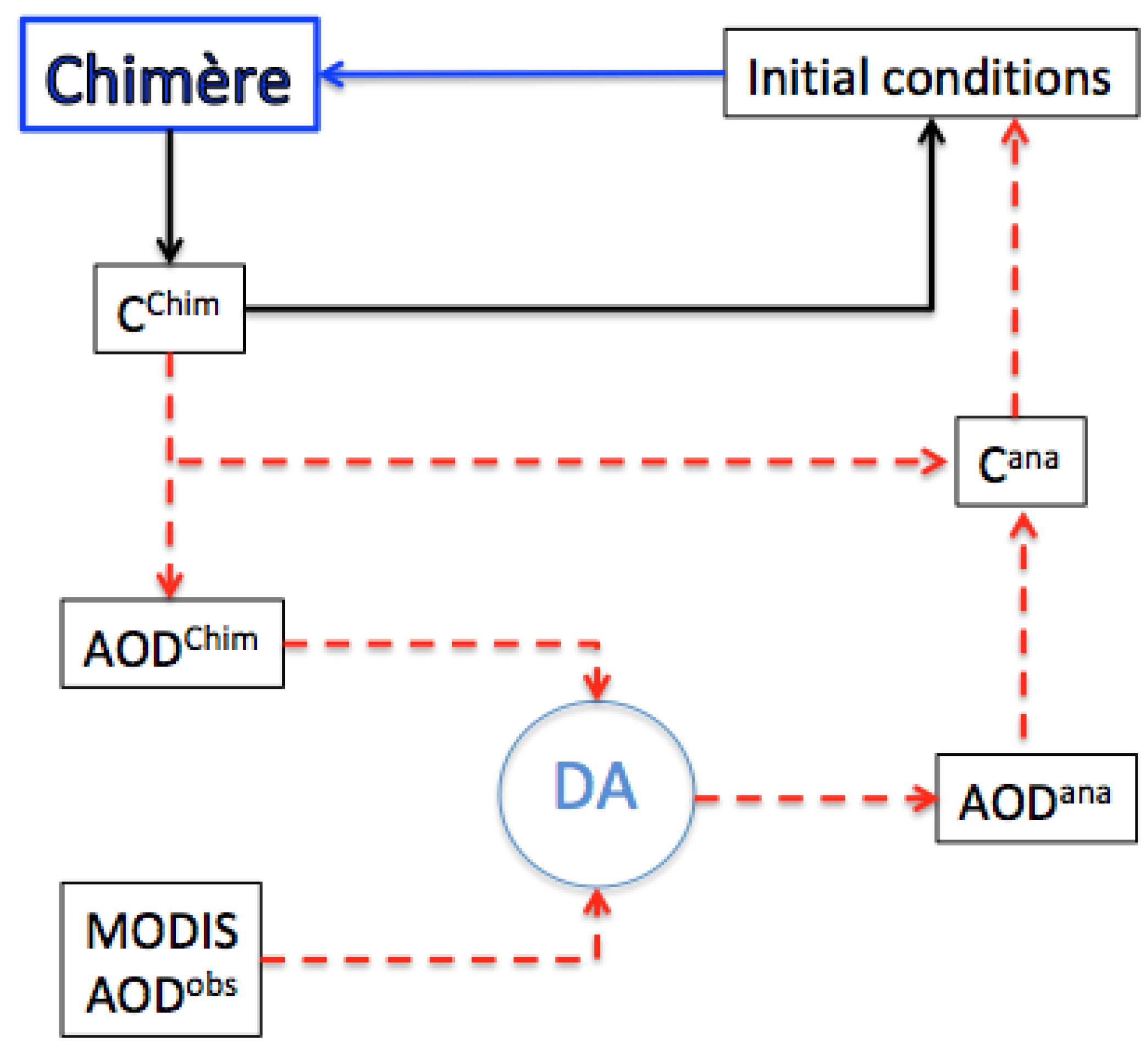
The default configuration of the model without DA consists of taking the initial concentration of a given species i, given size section j and at a given time step from the output concentration computed from the previous time step. The configuration with DA suggested in this study is based on a “Forecast-Analysis Cycling Scheme” and consists of using the model output AOD as the first guess and satellite AOD as input observations to generate the analysis of AOD, with which the model’s output concentrations are adjusted and fed back to the model as initial concentrations, instead of taking model output concentrations as the initial conditions, as shown in Figure 1.

The data assimilation system developed here is illustrated in Figure 1 and can be summarized in a set of three steps:

1

The AOD was computed from the modeled aerosol concentrations and taken as a first guess AOD${}^{Chim}$ at 00 UTC every day.

2

The analysis of AOD field AOD${}^{ana}$ was computed at 00 UTC from AOD${}^{Chim}$ and the retrieved AOD${}^{obs}$ covering Europe during the prior day using the OI described in Section 2.2.

3

The concentrations C${}_{i,j}^{Chim}$ that refer to the concentration of each chemical component i of PM${}_{2.5}$ at each size size bin j were updated at 00 UTC using an adjustment ratio (AOD${}^{ana}$/AOD${}^{Chim}$) shown in Section 2.2, and the analysis of concentrations were computed C${}_{i,j}^{ana}$, which refer to the analysis of the concentration of each component i of PM${}_{2.5}$ at each size bin j.

For each daily job run, the data assimilation covered the hours during which the satellite observations were available.

2.2. Objective Analysis of Satellite-Derived AOD

The Analysis-Forecast cycling scheme is based on adjusting the modeled concentrations with the ratio of the AOD analysis AOD${}^{ana}$ to modeled AOD${}^{Chim}$ as described by Equation (1). The fraction $\frac{{\mathrm{AOD}}^{ana}}{{\mathrm{AOD}}^{chim}}$ is considered the same for all concentrations in the vertical column volume:

$$C_{i,j}^{ana}=C_{i,j}^{chim}\times \frac{{\mathrm{AOD}}^{ana}}{{\mathrm{AOD}}^{chim}}$$

(1)

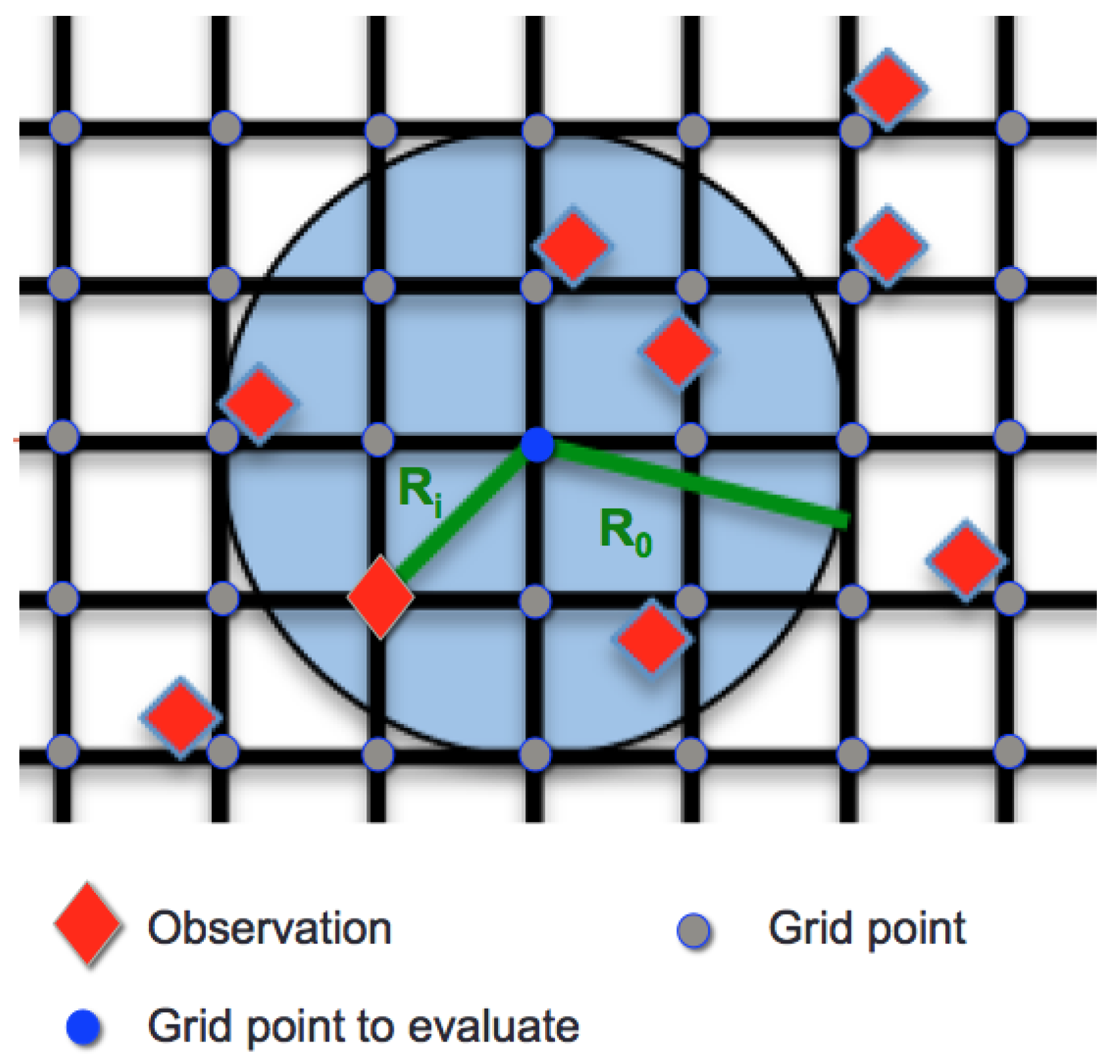
The objective analysis of AOD at a grid point m was performed by successive corrections using Equation (2). The successive correction method used in this work was the Creesman scheme, which uses satellite observations within a prescribed radius of influence as shown in Figure 2, and observations outside the influence radius were not used to assimilate the AOD field:

$$\begin{array}{c}{\mathrm{AOD}}_{m,0}^{ana}={\mathrm{AOD}}_m^{Chim}\hfill \\ {\mathrm{AOD}}_{m,n+1}^{ana}={\mathrm{AOD}}_{m,n}^{ana}+\frac{{\sum }_{k=1}^{k=K_{m,n}}{\alpha }_{m,k}^n({\mathrm{AOD}}_k^{obs}-{\mathrm{AOD}}_{k,n}^{ana})}{{\sum }_{k=1}^{k=K_n}{\alpha }_{m,k}^n+E^2}\hfill \end{array}$$

(2)

where AOD${}_k^{obs}$ is the kth observation surrounding the grid point m, AOD${}_m^{Chim}$ is the modeled AOD using Chimère (background) at the grid point m, AOD${}_{m,n}^{ana}$ is the nth iteration estimation of AOD${}^{ana}$ at the grid point m and AOD${}_{k,n}^{ana}$ is the nth estimate of AOD${}^{ana}$ evaluated at the observation point k. K${}_{m,n}$ refers to the index of the farthest cell within the influence circle of radius equal to the influence radius and centered on the grid point m. E${}^2$ is an estimate of the ratio of the observation error to the first guess field error. This value was assumed to be 10%. ${\alpha }_{m,k}^n$ is a weight function which depends on how far the observation m is from the grid point k, as shown Equation (3), where r${}_{m,k}$ is the distance between an observation point k and a grid point m. The radius of influence R${}_n$ was allowed to vary with the iteration by a constant factor R${}_{n+1}^2=\gamma$R${}_n^2$. The factor $\gamma$ was set to be less than 1 to reproduce the details in the observations field in the analysis field. Here, multiple values of the $\gamma$ factor of 0.8, 0.5 and 0.3 were tested and are equal to 0.3, so the observation minus analysis increments (O-A) were located over the observation locations.

In this approach, selecting the proper values of the radius of influence was somewhat empirical and depended upon the data spacing and the desired level of smoothing. Thiébaux and Pedder [39] showed that a radius of influence is approximately twice the average spacing of the observations in a time when Tombette et al. [25] used an influence radius of one mesh cell. These values tend to be a reasonable compromise between under-smoothing and over-smoothing. A radius of influence of one grid spacing was used as default, and a sensitivity study to the radius of influence using a radius of one grid cell and two grid cells was conducted in Section 4:

$${\alpha }_{m,k}^n=\left\{\begin{array}{c}\frac{R_n^2-r_{m,k}^2}{R_n^2+r_{m,k}^2}{r}_{m,k}^2<R_n^2\hfill \\ 0r_{m,k}^2\ge R_n^2\hfill \end{array}\right.$$

(3)

Using these types of functions, the grid point values reflected the observations in areas of high observation density, while in low-density areas, the grid values were closer to the first guess (modeled AOD).

2.3. Chimère Model Setup

The Chimère model (Menut et al. [40]; http://www.lmd.polytechnique.fr/chimere, accessed on 28 April 2022) was run to simulate the concentrations of particles and their composition in 2013 over Europe. The domain covered the area from 14${}^{\circ }$ W to 25${}^{\circ }$ E in longitude and from 35${}^{\circ }$ N to 58${}^{\circ }$ N in latitude with a 0.5${}^{\circ }\times$ 0.5${}^{\circ }$ of spatial resolution. There were 9 vertical levels up to 500 hPa. The Chimèe model needs a set of gridded input data: meteorological data, sea salt, biogenic and anthropogenic emissions, land use parameters, initial and boundary conditions and deposition velocities.

Meteorology was obtained from the Weather Research and Forecasting model (WRF) regional model forced by NCEP (National Centers of Environmental Predictions, http://www.ncep.noaa.gov, (accessed on 28 April 2022) with a base resolution of 1${}^{\circ }$. The online coupling mode Chimèe-WRF was used here with a feedback of the aerosol optical properties to induce a radiative forcing, as shown in Briant et al. [41].

Annual anthropogenic emissions of gases and particles were taken from the EMEP inventory for 2009. Temporalization of emissions was performed according to temporal factors for each country provided by GENEMIS [42].

Biogenic emissions were computed with the Model of Emissions and Gases and Aerosols from Nature (MEGAN) 2.1 [43] with high-resolution emission factors and leaf area index (LAI) data. These emissions from biogenic sources included isoprene, limonene, $\alpha$-pinene, $\beta$-pinene, humulene and ocimene. Sea-salt emissions were computed according to Monahan et al. [44].

Boundary conditions were generated from the results of the Model for OZone And Related chemical Tracers (MOZART v4.0; Emmons et al. [45]) available online at https://www.acom.ucar.edu/wrf-chem/mozart.shtml (accessed on 28 April 2022). Initial conditions of chemical species were taken from the GOCART model [46].

The MELCHIOR2 [47] mechanism was used to simulate the gas-phase chemistry.

Evaporation/condensation of semi-volatile species was represented with the algorithm of Pandis et al. [48] using thermodynamic equilibria. Coagulation of particles was represented as in Debry et al. [49]. Thermodynamic equilibria were computed with the ISORROPIA II model [50] for inorganic compounds. Ten bins for aerosol size distribution and the SOA (secondary organic aerosols) scheme of Bessagnet et al. [51] were used here. The Chimere aerosol module distributes aerosols in 10 size bins ranging from 40 nm to 40 $\mathsf{\mu }$m in a logarithmic sectional approach.

The Wesely [52] aerosol dry deposition and Loosmore [53] resuspension schemes were used. The online coupling with the ISORROPIA model was used.

The basic chemical speciation includes elemental carbon, sulfate, nitrate, ammonium, sodium, chloride, dust, SOA (formed from biogenic and anthropogenic VOCs and primary organic aerosol) and the primary particulate matter other than ones mentioned above.

2.4. Observation Data

2.4.1. MODIS Data

MODIS products used in this study were a composite of AOD from MODIS TERRA (north to south transect at about 10:30 a.m. local time) and MODIS AQUA (south to north orbital transect about 1:30 p.m. local time) products. Both Terra- and Aqua-MODIS instruments view the entire Earth’s surface every 1 to 2 days, acquiring data in 36 spectral bands ranging in wavelengths from 0.4 to 14.4 $\mathsf{\mu }$m. AOD retrievals were calculated at 0.55 $\mathsf{\mu }$m (AOD${}_{550}$) and originally processed using MODIS data at a spatial resolution of 0.1${}^{\circ }$× 0.1${}^{\circ }$. The MODIS AOD field was projected to the 0.5${}^{\circ }$× 0.5${}^{\circ }$ spatial longitude/latitude grid and happened to be only available in a subset of observation pixels due to multiple reflective surfaces and cloud contamination.

2.4.2. AERONET Data

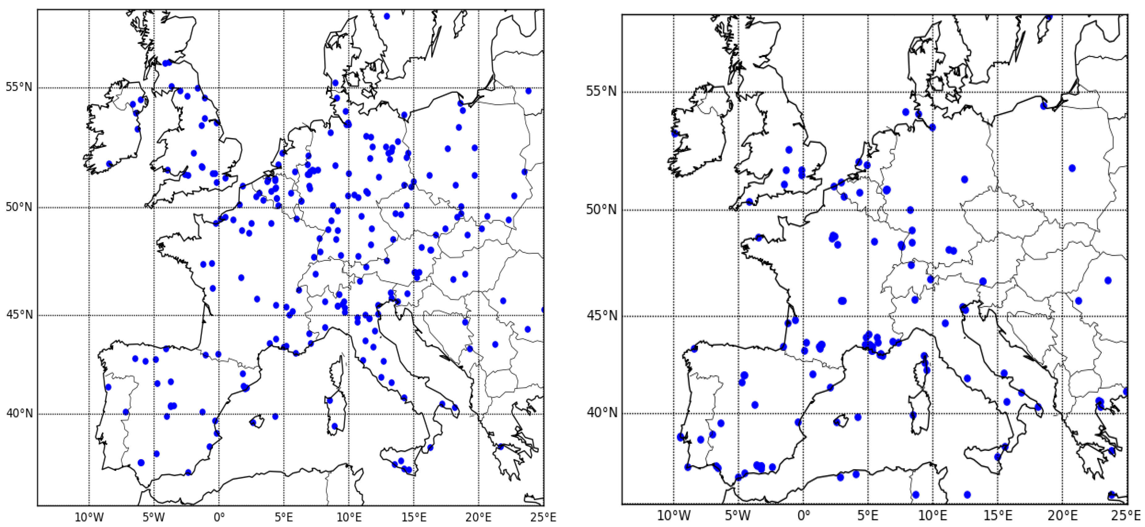
The AERONET (AErosol RObotic NETwork) photometers measurements [54,55] were used to characterize the observed AOD. The AOD data were recorded by numerous stations deployed around the world, and hourly values are available in https://aeronet.gsfc.nasa.gov/new_web/aerosols.html (accessed on 28 April 2022). Several quality levels were proposed on the AERONET database. In this study, the level 2.0 AERONET AOD at 440 and 870 nm and Ångström Exponent (AE${}_{440/870}$) [56] with an uncertainty estimated to less than 0.02 [4,55] were used to derive AOD at 550 nm using logarithmic interpolation. If an AOD value was not available at 440 nm, then the AOD was not obtained at 550 nm. If the AOD at 870 nm was not available, the interpolation is made between AOD at 440 and 1020 nm. The location of the stations are displayed in Figure 3.

2.4.3. AirBase Data

AirBase (https://www.eea.europa.eu/data-and-maps/data/airbase-the-european-air-quality-database-8, accessed on 28 April 2022) gathers regulatory data reported by Member States of the European Union according to the air quality directives [57]. For this study, quality-controlled and assured hourly PM${}_{2.5}$ data from both rural and urban background stations were used. Figure 3 shows the locations of the AirBase stations over Europe used here.

2.5. Statistical Evaluation Method

The statistical evaluation was based on a set of performance statistical indicators: the simulated mean ($\overline{s}$), the root mean square error (RMSE), the correlation coefficient, the mean fractional bias (MFB) and the mean fractional error (MFE). They are defined in

Table 1. Definitions of the statistics used in this work. ${\left(o_i\right)}_i$ and ${\left(c_i\right)}_i$ are the observed and the simulated concentrations at time and location i, respectively. n is the number of data.

Statistic Indicator	Definition
Root mean square error (RMSE)	$\sqrt{{\displaystyle \frac{1}{n}}{\sum }_{i=1}^n{(c_i-o_i)}^2}$
Correlation (Corr)	${\displaystyle \frac{{\sum }_{i=1}^n(c_i-\overline{c})(o_i-\overline{o)}}{\sqrt{{\sum }_{i=1}^n{(c_i-\overline{c})}^2}\sqrt{{\sum }_{i=1}^n{(o_i-\overline{o})}^2}}}$
Mean fractional bias (MFB)	${\displaystyle \frac{1}{n}}{\sum }_{i=1}^n{\displaystyle \frac{c_i-o_i}{(c_i+o_i)/2}}$
Mean fractional error (MFE)	${\displaystyle \frac{1}{n}}{\sum }_{i=1}^n{\displaystyle \frac{\mid c_i-o_i\mid }{(c_i+o_i)/2}}$

. Based on the MFB and the MFE, Boylan and Russell [58] proposed a performance and a goal evaluation criteria as detailed in

Table 2. Boylan and Russel criteria.

Criteria	Performance Criterion	Goal Criterion
|MFB|	≤60%	≤30%
MFE	≤75%	≤50%

.

2.6. An Analysis Example

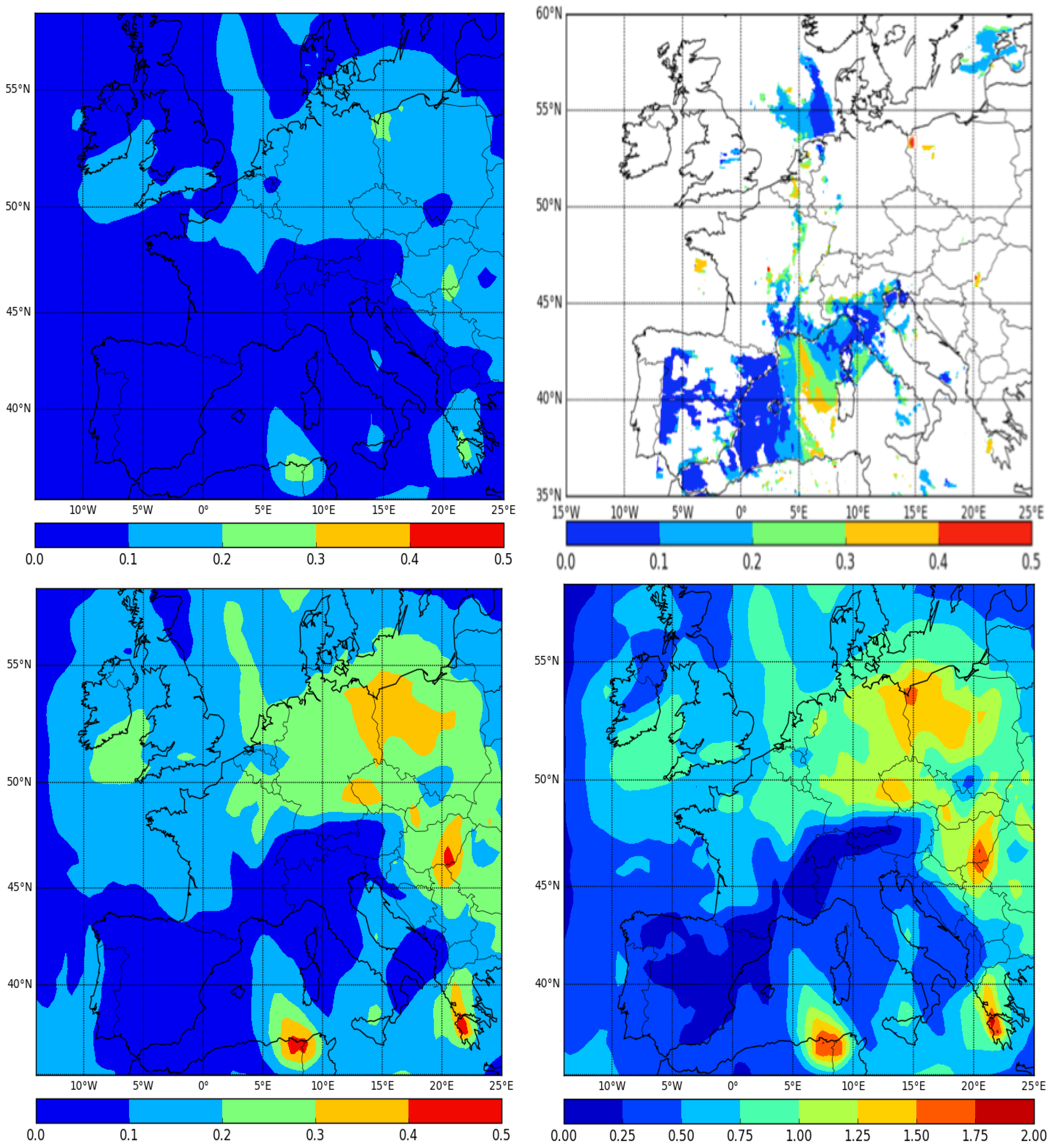
An example of the calculation of the analysis of AOD field for the first simulation day of 7 March 2009 is shown in this section. All MODIS observations during a day were assimilated at 00 UTC: the MODIS observations at 1:30 Local Time were assimilated at 00UTC. The modeled, retrieved and the analyzed AOD fields during that day are shown in Figure 4.

On 7 March 2009, the MODIS data were not available over the whole European domain because of the cloud coverage during a winter day. The model tends to underestimate the AOD over areas where satellite data are available (a bias of −69% is found over the cells where MODIS data is available). The modeled AOD values did not exceed 0.3. The analysis of AOD field showed higher values especially over Tunisia, Greece, south of France and Eastern Europe due to the impact of high observed AOD values.

A map of the adjustment ratio (AOD${}^{ana}$/AOD${}^{Chim}$) is shown in Figure 4.

Figure 4 shows that this adjustment ratio locally exceeds 1.0, especially over regions where the satellite AOD are available.

3. Simulations Experiments Evaluation

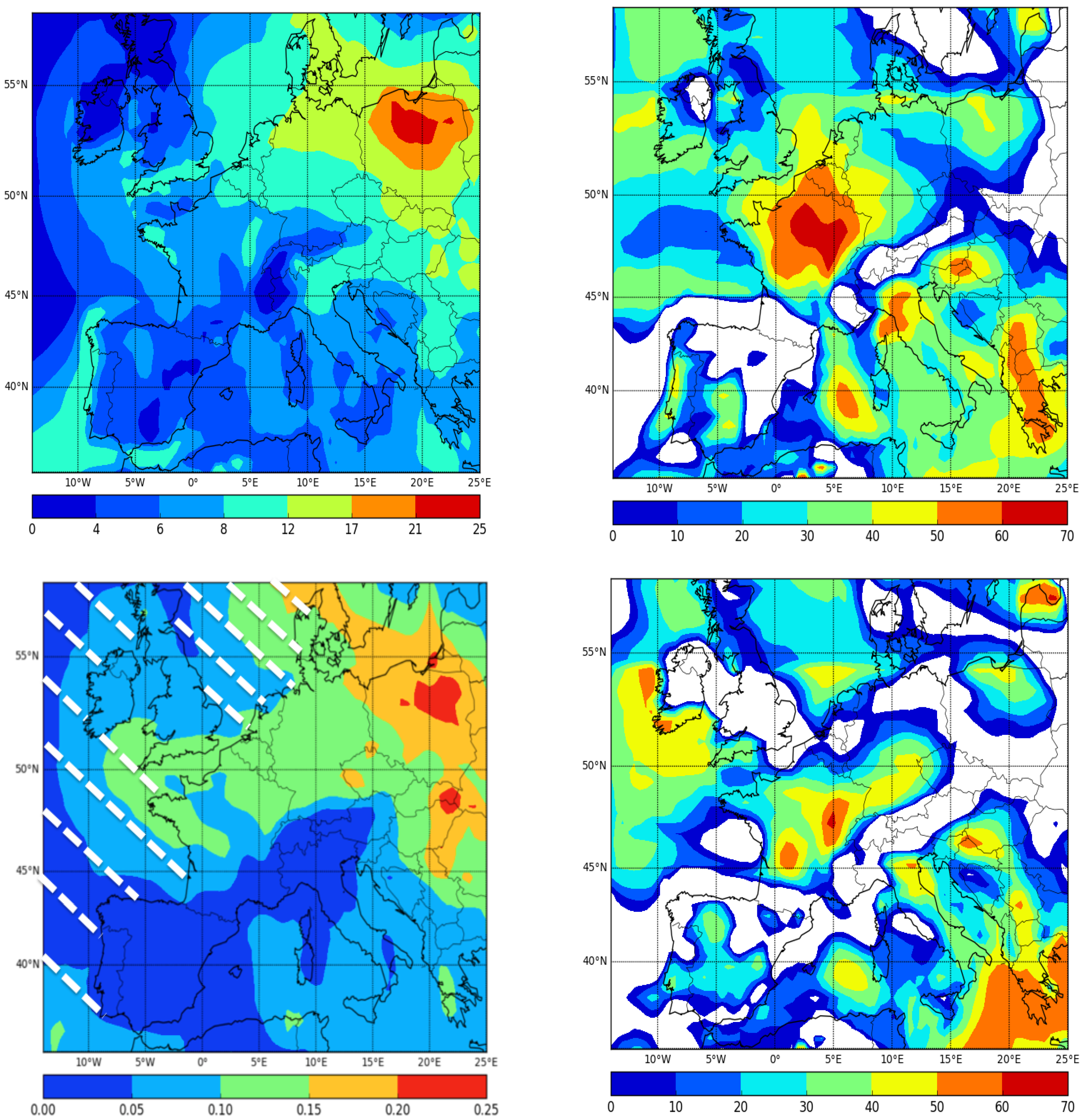
Two simulations are performed with the same input data and parameterizations during the month of March 2009, which correspond to record pollution concentrations over Europe: the first one is the reference simulation without DA (called “Simulation without D.A.”), and the second one is run with the developed DA (called “Simulation with D.A.”). Figure 5 shows maps of PM${}_{2.5}$ concentrations and AOD field over Europe averaged over March 2009 and the relative difference between the two simulations in order to quantify the impact of OA on the model predictions. The white areas in Figure 5 correspond to areas of relative difference equal to zero.

The effect of OA during the one-month period is significant. The main differences between the modeled concentrations of PM${}_{2.5}$ and AOD with and without OA are located over France (∼50–60%) and the southern part of Europe (∼50–60%): the northern part of Italy, Balkans, south of Greece and over the Mediterranean.

The modeled PM${}_{2.5}$ concentrations (resp. AOD) are compared against hourly surface observations from AirBase (resp. AERONET) network in

Table 3. Statistics of model to AirBase measurements comparisons for hourly PM${}_{2.5}$ concentrations during March 2009. $\overline{s}$ and RMSE are expressed in $\mathsf{\mu }$g·m${}^{-3}$.

$\overline{\mathit{o}}$ = 38.01 $\mathsf{\mu }$g·m${}^{-3}$	$\overline{\mathit{s}}$	RMSE	Correlation [%]	MFB [%]	MFE [%]
Simulation without D.A.	20.89	30.05	40	$-34$	51
Simulation with D.A.	33.21	15.13	45	$-15$	39

(resp.

Table 4. Statistics of model to AERONET measurements comparisons for daily AOD during March 2009. $\overline{s}$ and RMSE are expressed in $\mathsf{\mu }$g·m${}^{-3}$.

$\overline{\mathit{o}}$ = 0.37	$\overline{\mathit{s}}$	RMSE	Correlation [%]	MFB [%]	MFE [%]
Simulation without D.A.	0.21	0.19	73	$-45$	55
Simulation with D.A.	0.30	0.11	78	$-27$	42

).

Using the default simulation without the DA, the modeled surface concentrations of PM${}_{2.5}$ are significantly underestimated by a factor of about 47% (the measured and modeled means are 38.01 and 20.01 $\mathsf{\mu }$g·m${}^{-3}$, respectively). The goal criteria are not respected as the mean fractional bias and error are $-34$ and 51%, respectively. This underestimation is mainly due to the fact that the model highly underestimates PM${}_{2.5}$ concentrations over the urban background stations but modeled PM${}_{2.5}$ concentrations agree better with the observed concentrations over the rural background. The reasons of this underestimation were explained by Terrenoire et al. [59] who showed Chimère has more difficulty in reproducing the PM concentrations during winter, especially at urban background stations because the model is not able to correctly simulate the stable meteorological conditions that lead to high PM episodes [60].

During this winter month, PM${}_{2.5}$ are mainly composed of primary organic compounds mainly emitted by industrial, traffic and biomass-burning anthropogenic sectors. The highest concentrations are located over North Eastern Europe, which is consistent with results found by Terrenoire et al. [59].

Because of the OA, PM${}_{2.5}$ concentrations increased by 59% as the simulated means moved from 20.89 to 33.21 $\mathsf{\mu }$g·m${}^{-3}$ and became closer to the observed mean (38.01 $\mathsf{\mu }$g·m${}^{-3}$). The RMSE also decreased from 30.05 to 15.13 $\mathsf{\mu }$g·m${}^{-3}$. The bias and error, moreover, were reduced from $-34$ to $-14$% and from 51 to 39%, respectively.

In addition, the model performance improved as the modeled PM${}_{2.5}$ concentrations using OA respect the goal criterion in a time when the modeled concentrations without OA respects only the performance criterion. Tombette et al. [25] evaluated the OA effect using Polyphemus model on both PM${}_{10}$ and PM${}_{2.5}$ over 156 European stations and found that PM${}_{10}$ concentrations increased by 7% and the bias was reduced from 55% to 49%, and over 8 European stations, PM${}_{2.5}$ concentrations increased by a factor of 7%. Tang et al. [35] also improved hourly PM${}_{2.5}$ and ozone concentrations using OA over AIRNOW measurements as the mean bias improved from $-7.14$ to $-0.11$ $\mathsf{\mu }$g·m${}^{-3}$ and from 2.54 to 1.06 ppbV.

Similarly, the modeled AOD field over AERONET stations increased by a factor of 43% from 0.21 to 0.30. The correlation also slightly improved from 73 to 78%. Both the bias and error decreased from −45 to −27% and from 55 to 42%. The error of 42% can be explained by the fact that AERONET can make a much wider range of measurements throughout the day while MODIS onboard Terra and Aqua pass at 10:30 and 1:30 local time, respectively.

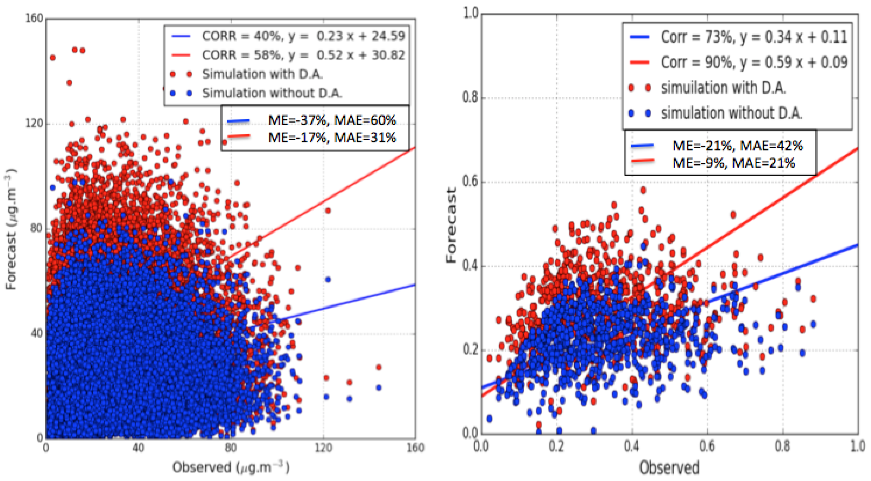
Figure 6 shows the scatter plots of hourly PM${}_{2.5}$ concentrations and AOD modeled with and without the developed DA over AirBase and AERONET stations, respectively.

The number of compared data in the AERONET network is lower than the number of compared AirBase data because numerous missing data were found in the AERONET data. The correlation moved from 40 to 58%, and the slope of the scatter plot increased from 0.23 to 0.52. The same result is found when it comes to the modeled AOD (as the correlation increased from 73 to 90% and the slope of the scatter plot moved from 0.34 to 0.59). The analysis fields show an overestimation of the PM${}_{2.5}$ concentrations. This overestimation (false alarms) can be explained by the fact that concentrations of PM with an aerodynamic diameter larger than 2.5 $\mathsf{\mu }$m are also sensitive to AOD${}_{550}$ and therefore are accounted for in Equation (1). A better distribution of AOD by particles size should be added to avoid false alarms in the forecasting system in future studies. In addition, the model was evaluated against the terrestrial part of the simulated domain as shown in Figure 5. Because of the diurnal change in the boundary layer, as well as humidity and other factors that are very different over the sea surface than the terrestrial surface, this evaluation of the model and the DA impact needs to be further validated over the part of the Atlantic Ocean of the domain (dashed area in Figure 5). Over the Mediterranean sea, the AirBase and AERONET stations over islands such as Corsica, Malta, the Balearic Islands, etc., can be considered as a validation over the Mediterranean sea.

Temporal Impact of the OA

In order to evaluate the effectiveness of the MODIS AOD assimilation, the time scale for which the OA affects the concentrations is worth exploring because the OA operates on the initial conditions. Figure 7 shows the hourly evolution of PM${}_{2.5}$ concentrations averaged over all grid points where the relative difference is over 20% to better estimate the influence of the DA. Figure 7 shows that the effect of OA lasts nearly 13 h, which is comparable to the temporal impact found by Tombette et al. [25] using OA along with Polyphemus model over Europe. After 13 h, the impact of the MODIS data on the modeled concentrations is low because the impact of the regional transport and local emissions start overshadowing the assimilation impact.

4. Sensitivity to the Creesman Influence Radius

The performance of the OA is tested using two different influence radii. A first (resp. second) simulation using an influence radius R${}_1$ (R${}_2$) equal to (is twice) the grid cell spacing, which corresponds to 0.5${}^{\circ }$ (1${}^{\circ }$).

Table 5. Temporal and spatial sum of relative differences between the simulations whereby the influence radius is set to twice and equal to the average spacing of observations.

Influence Radius	Relative Difference (%)
PM${}_{2.5}$	10.2
AOD	12.3

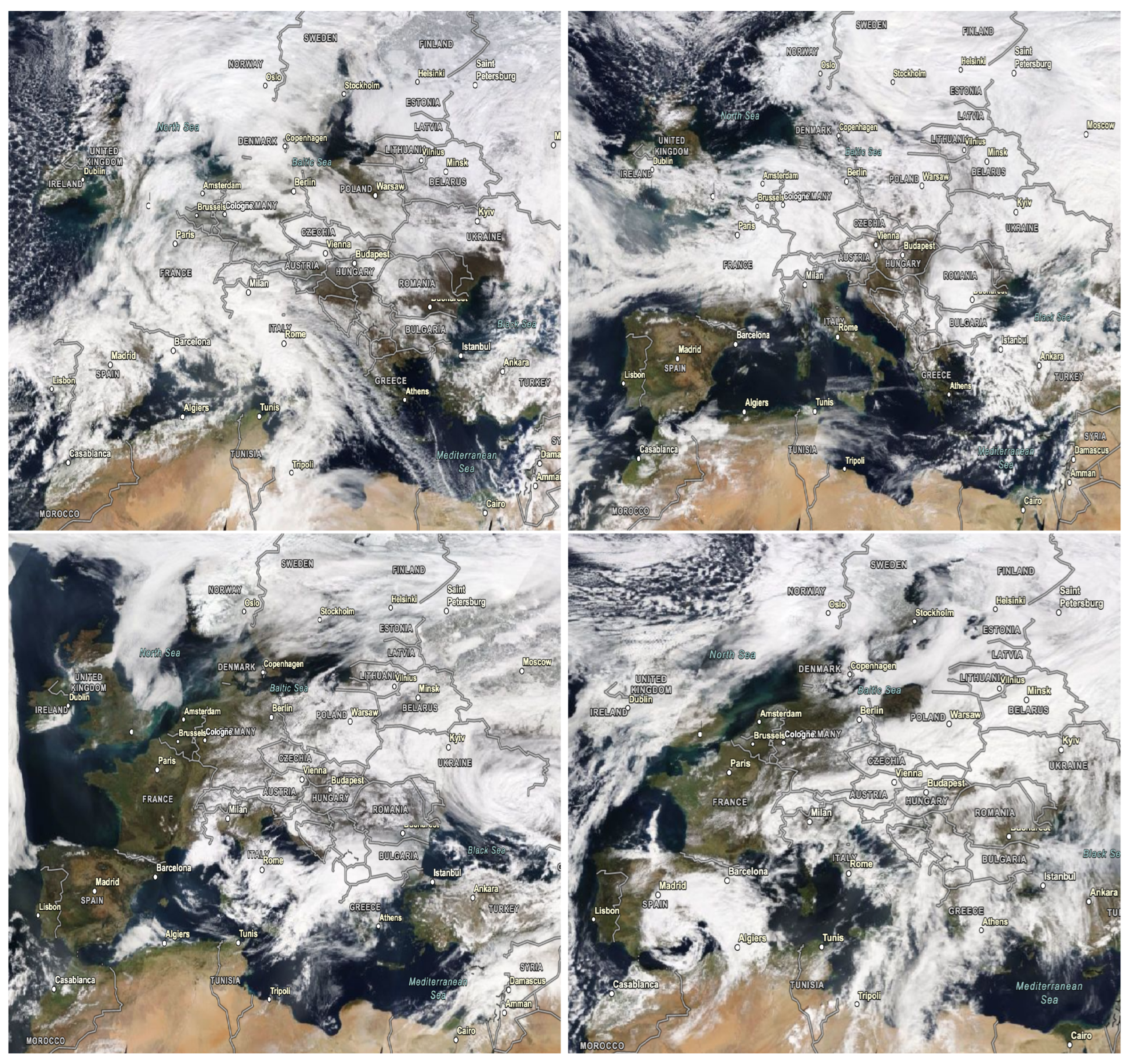
shows the temporal and spatial sum of relative differences between the simulations with OA computed with R${}_1$ and R${}_2$, respectively, over the cells where the effect of OI exceeds 20%. The comparison shows that the model performance is slightly sensitive to the influence radius value: the relative difference between the two simulations do not exceed 10.5 (12.3)% for PM${}_{2.5}$ concentrations (AOD). This may be due to the low satellite observation density during winter because of dense cloud coverage. Figure 8 shows the cloud coverage (MODIS Terra-corrected reflectance with a spatial resolution of 250 m) over Europe on four different days in March as examples of where the majority of the European land is masked by clouds. The results are expected to be more sensitive to the influence radius if the satellite data were of better quality or obtained during summertime.

The comparison of the two simulations against AirBase and AERONET data in

Table 6. Statistics of hourly simulated PM${}_{2.5}$ concentrations with DA using two influence radii R${}_1$ and R${}_2$ to AirBase measurements comparisons during March 2009. $\overline{s}$ and RMSE are expressed in $\mathsf{\mu }$g·m${}^{-3}$.

$\overline{\mathit{o}}$= 38.01 $\mathsf{\mu }$g·m${}^{-3}$	$\overline{\mathit{s}}$	RMSE	Correlation [%]	MFB [%]	MFE [%]
Simulation with DA (R${}_1$)	33.21	15.13	45	$-15$	39
Simulation with DA (R${}_2$)	29.44	20.71	40	$-31$	51

and

Table 7. Statistics of hourly simulated AOD with DA using two influence radii R${}_1$ and R${}_2$ to AERONET measurements comparisons for daily AOD during March 2009. $\overline{s}$ and RMSE are expressed in $\mathsf{\mu }$g·m${}^{-3}$.

$\overline{\mathit{o}}$ = 0.37	$\overline{\mathit{s}}$	RMSE	Correlation [%]	MFB [%]	MFE [%]
Simulation with DA (R${}_1$)	0.30	0.11	78	$-27$	42
Simulation with DA (R${}_2$)	0.25	0.31	65	$-54$	72

show that simulation with a radius of influence equal to the grid cell predicts PM${}_{2.5}$ and AOD that have a better agreement with observations. The simulated mean of PM${}_{2.5}$ concentrations (AOD) 33.21 $\mathsf{\mu }$g·m${}^{-3}$ (0.30) are closer to the observed means 38.01 $\mathsf{\mu }$g·m${}^{-3}$ (0.37). In addition, the goal criteria are respected with the analysis of the PM${}_{2.5}$ concentration field simulated using R${}_1$.

5. Conclusions

In this study, we tested the assimilation method of objective analysis to adjust Chimère’s initial conditions for the simulation of PM${}_{2.5}$ and AOD${}_{550}$ over Europe during March 2009. The base model underestimated surface PM${}_{2.5}$ concentrations and AOD field because of the low resolution and uncertainties on meteorology and emissions. The objective analysis assimilation was able to correct the aerosol concentrations and AOD fields. However, the impact of adjusting initial conditions can be overshadowed by the local emissions and local winds, as they lasted for 13 h. The proposed model can be used in operational air quality forecasting, data validation and the verification of regulations.

Assimilating data from elevated levels or airborne measurements, although occasionally available, can be used to sharpen the adjustment of initial conditions and would improve PM${}_{2.5}$ concentration and AOD field as it represents the loading of the aerosol column. However, precise knowledge on the vertical distribution of PM${}_{2.5}$ using lidars [61,62] is required for at least two reasons: (1) it is better for quantifying air quality and its variability since, for example, the different vertical distribution of PM${}_{2.5}$ near the Earth surface has very different impact on public health; (2) it is likely to significantly enhance the PM${}_{2.5}$ estimation and provide data for model evaluation, improvement and development for the daily air quality forecast.

Future works could focus on investigating the OA impact on finer-resolution simulations, describing the background and observation covariance matrices better, using more complex data assimilation techniques such as 4D-var and ensemble Kalman filter, describing the emissions using a top-down approach (inverse modeling) better, combining the use of satellite data with ground based or airborne observations of the aerosol chemical composition (organics, sulfate, nitrate, sea-salts, etc.). The use of lidar observations could furthermore be very beneficial to improve the vertical distribution of aerosols.

References

1. Bigi, A.; Ghermandi, G. Trends and variability of atmospheric PM2.5 and PM10–2.5 concentration in the Po Valley, Italy. Atmos. Chem. Phys. 2016, 16, 15777–15788. [Google Scholar] [CrossRef] [Green Version]
2. Barmpadimos, I.; Keller, J.; Oderbolz, D.; Hueglin, C.; Prévôt, A.S.H. One decade of parallel fine (PM2.5) and coarse (PM10 – PM2.5) particulate matter measurements in Europe: Trends and variability. Atmos. Chem. Phys. 2012, 12, 3189–3203. [Google Scholar] [CrossRef] [Green Version]
3. Van Loon, M.; Roemer, M.; Builtjes, P. Model Intercomparison in the Framework of the Review of the Unified EMEP Model; TNO Environment Energy and Process Innovation, TNO Report—R2004/282; TNO-MEPO-R 2004/282: The Hauge, The Netherlands, 2004. [Google Scholar]
4. Majdi, M.; Turquety, S.; Sartelet, K.; Legorgeu, C.; Menut, L.; Kim, Y. Impact of wildfires on particulate matter in the Euro-Mediterranean in 2007: Sensitivity to the parameterization of emissions in air quality models. Atmos. Chem. Phys. Discuss. 2018, 2018, 1–32. [Google Scholar] [CrossRef] [Green Version]
5. He, C.; Li, Q.B.; Liou, K.N.; Zhang, J.; Qi, L.; Mao, Y.; Gao, M.; Lu, Z.; Streets, D.G.; Zhang, Q.; et al. A global 3-D CTM evaluation of black carbon in the Tibetan Plateau. Atmos. Chem. Phys. 2014, 14, 7091–7112. [Google Scholar] [CrossRef] [Green Version]
6. Prank, M.; Sofiev, M.; Tsyro, S.; Hendriks, C.; Semeena, V.; Vazhappilly Francis, X.; Butler, T.; Denier van der Gon, H.; Friedrich, R.; Hendricks, J.; et al. Evaluation of the performance of four chemical transport models in predicting the aerosol chemical composition in Europe in 2005. Atmos. Chem. Phys. 2016, 16, 6041–6070. [Google Scholar] [CrossRef] [Green Version]
7. Chrit, M.; Sartelet, K.; Sciare, J.; Pey, J.; Nicolas, J.B.; Marchand, N.; Freney, E.; Sellegri, K.; Beekmann, M.; Dulac, F. Aerosol sources in the western Mediterranean during summertime: A model-based approach. Atmos. Chem. Phys. 2018, 18, 9631–9659. [Google Scholar] [CrossRef] [Green Version]
8. Nilsson, E.D.; Rannik, U.; Buzorius, G.; Kulmala, M.; O’Dowd, C. Effects of the continental boundary layer evolution, convection, turbulence and entrainment on aerosol formation. Tellus B 2001, 53, 441–461. [Google Scholar] [CrossRef]
9. Aan de Brugh, J.M.J.; Henzing, J.S.; Schaap, M.; Morgan, W.T.; van Heerwaarden, C.C.; Weijers, E.P.; Coe, H.; Krol, M.C. Modelling the partitioning of ammonium nitrate in the convective boundary layer. Atmos. Chem. Phys. 2012, 12, 3005–3023. [Google Scholar] [CrossRef] [Green Version]
10. Ervens, B.; Turpin, B.J.; Weber, R.J. Secondary organic aerosol formation in cloud droplets and aqueous particles (aqSOA): A review of laboratory, field and model studies. Atmos. Chem. Phys. 2011, 11, 11069–11102. [Google Scholar] [CrossRef] [Green Version]
11. Chrit, M.; Sartelet, K.; Sciare, J.; Majdi, M.; Nicolas, J.; Petit, J.E.; Dulac, F. Modeling organic aerosol concentrations and properties during winter 2014 in the northwestern Mediterranean region. Atmos. Chem. Phys. Discuss. 2018, 2018, 1–28. [Google Scholar] [CrossRef] [Green Version]
12. Feng, Y.; Penner, J.E.; Sillman, S.; Liu, X. Effects of cloud overlap in photochemical models. J. Geophys. Res. 2004, 109, D04310. [Google Scholar] [CrossRef] [Green Version]
13. Roustan, Y.; Sartelet, K.; Tombette, M.; Debry, É.; Sportisse, B. Simulation of aerosols and gas-phase species over Europe with the Polyphemus system. Part II: Model sensitivity analysis for 2001. Atmos. Env. 2010, 44, 4219–4229. [Google Scholar] [CrossRef]
14. Bocquet, M.; Elbern, H.; Eskes, H.; Hirtl, M.; Žabkar, R.; Carmichael, G.R.; Flemming, J.; Inness, A.; Pagowski, M.; Pérez Camaño, J.L.; et al. Data assimilation in atmospheric chemistry models: Current status and future prospects for coupled chemistry meteorology models. Atmos. Chem. Phys. 2015, 15, 5325–5358. [Google Scholar] [CrossRef] [Green Version]
15. Segers, A. Data Assimilation in Atmospheric Chemistry Models Using Kalman Filtering. Ph.D. Thesis, Delft University of Technology, Delft, The Netherlands, 2002. [Google Scholar]
16. Wu, L.; Mallet, V.; Bocquet, M.; Sportisse, B. A comparison study of data assimilation algorithms for ozone forecasts. J. Geophys. Res. 2008, 113, D20310. [Google Scholar] [CrossRef] [Green Version]
17. Sandu, I.; Stevens, B.; Pincus, R. On the transitions in marine boundary layer cloudiness. Atmos. Chem. Phys. 2010, 10, 2377–2391. [Google Scholar] [CrossRef] [Green Version]
18. Hu, Y.; Zang, Z.; Chen, D.; Ma, X.; Liang, Y.; You, W.; Pan, X.; Wang, L.; Wang, D.; Zhang, Z. Optimization and Evaluation of SO2 Emissions Based on WRF-Chem and 3DVAR Data Assimilation. Remote Sens. 2022, 14, 220. [Google Scholar] [CrossRef]
19. Sekiya, T.; Miyazaki, K.; Ogochi, K.; Sudo, K.; Takigawa, M.; Eskes, H.; Boersma, K.F. Impacts of Horizontal Resolution on Global Data Assimilation of Satellite Measurements for Tropospheric Chemistry Analysis. J. Adv. Model. Earth Syst. 2021, 13, e2020MS002180. [Google Scholar] [CrossRef]
20. Liang, Y.; Zang, Z.; Liu, D.; Yan, P.; Hu, Y.; Zhou, Y.; You, W. Development of a three-dimensional variational assimilation system for lidar profile data based on a size-resolved aerosol model in WRF–Chem model v3.9.1 and its application in PM2.5 forecasts across China. Geosci. Model Dev. 2020, 13, 6285–6301. [Google Scholar] [CrossRef]
21. Schwartz, C.S.; Liu, Z.; Lin, H.C.; Cetola, J.D. Assimilating aerosol observations with a “hybrid” variational-ensemble data assimilation system. J. Geophys. Res. Atmos. 2014, 119, 4043–4069. [Google Scholar] [CrossRef]
22. Lee, E.H.; Ha, J.C.; Lee, S.S.; Chun, Y. PM10 data assimilation over south Korea to Asian dust forecasting model with the optimal interpolation method. Asia-Pac. J. Atmos. Sci. 2013, 49, 73–85. [Google Scholar] [CrossRef]
23. Pagowski, M.; Grell, G.A. Experiments with the assimilation of fine aerosols using an ensemble Kalman filter. J. Geophys. Res. Atmos. 2012, 117. [Google Scholar] [CrossRef]
24. Wang, Y.; Sartelet, K.N.; Bocquet, M.; Chazette, P. Assimilation of ground versus lidar observations for PM10 forecasting. Atmos. Chem. Phys. 2013, 13, 269–283. [Google Scholar] [CrossRef] [Green Version]
25. Tombette, M.; Mallet, V.; Sportisse, B. PM10 data assimilation over Europe with the optimal interpolation method. Atmos. Chem. Phys. 2009, 9, 57–70. [Google Scholar] [CrossRef] [Green Version]
26. Kumar, U.; De Ridder, K.; Lefebvre, W.; Janssen, S. Data assimilation of surface air pollutants (O3 and NO2) in the regionalscale air quality model AURORA. Atmos. Environ. 2012, 60, 99–108. [Google Scholar] [CrossRef]
27. Agudelo, O.M.; Viaene, P.; De Moor, B. Improving the PM10 estimates of the air quality model AURORA by using Optimal Interpolation. Atmos. Environ. 2015, 48, 1154–1159. [Google Scholar] [CrossRef]
28. Kalnay, E. Atmospheric Modeling, Data Assimilation, and Predictability; Cambridge University Press: Cambridge, UK, 2003. [Google Scholar]
29. Benedetti, A.; Fisher, M. Background error statistics for aerosols. Q. J. R. Meteorol. Soc. 2007, 133, 391–405. [Google Scholar] [CrossRef]
30. Benedetti, A.; Morcrette, J.J.; Boucher, O.; Dethof, A.; Engelen, R.J.; Fisher, M.; Flentje, H.; Huneeus, N.; Jones, L.; Kaiser, J.W.; et al. Aerosol analysis and forecast in the European Centre for Medium-Range Weather Forecasts Integrated Forecast System: 2. Data assimilation. J. Geophys. Res. Atmos. 2009, 114, D13205. [Google Scholar] [CrossRef] [Green Version]
31. Sugimoto, N.; Uno, I. Observation of Asian dust and air-pollution aerosols using a network of ground-based lidars (ADNet): Realtime data processing for validation/assimilation of chemical transport models. IOP Conf. Ser. Earth Environ. Sci. 2009, 7, 012003. [Google Scholar] [CrossRef]
32. Denby, B.; Schaap, M.; Segers, A.; Builtjes, P.; Horálek, J. Comparison of data assimilation methods for assessing PM10 exceedances on the European scale. Atmos. Environ. 2008, 42, 7122–7134. [Google Scholar] [CrossRef]
33. Candiani, G.; Carnevale, C.; Finzi, G.; Pisoni, E.; Volta, M. A comparison of reanalysis techniques: Applying optimal interpolation and Ensemble Kalman Filtering to improve air quality monitoring at mesoscale. Sci. Total Environ. 2013, 458, 7–14. [Google Scholar] [CrossRef]
34. Tang, Y.; Pagowski, M.; Chai, T.; Pan, L.; Lee, P.; Baker, B.; Kumar, R.; Delle Monache, L.; Tong, D.; Kim, H.C. A case study of aerosol data assimilation with the Community Multi-scale Air Quality Model over the contiguous United States using 3D-Var and optimal interpolation methods. Geosci. Model Dev. 2017, 10, 4743–4758. [Google Scholar] [CrossRef] [Green Version]
35. Tang, Y.; Chai, T.; Pan, L.; Lee, P.; Tong, D.; Kim, H.C.; Chen, W. Using optimal interpolation to assimilate surface measurements and satellite AOD for ozone and PM2.5: A case study for July 2011. J. Air. Waste Manag. 2015, 65, 1206–1216. [Google Scholar] [CrossRef] [PubMed] [Green Version]
36. Kaufman, Y.J.; Holben, B.N.; Tanré, D.; Slutsker, I.; Smirnov, A.; Eck, T.F. Will aerosol measurements from Terra and Aqua Polar Orbiting satellites represent the daily aerosol abundance and properties? Geophys. Res. Lett. 2000, 27, 3861–3864. [Google Scholar] [CrossRef]
37. Adhikary, B.; Kulkarni, S.; Dallura, A.; Tang, Y.; Chai, T.; Leung, L.R.; Qian, Y.; Chung, C.E.; Ramanathan, V.; Carmichael, G.R. A regional scale chemical transport modeling of Asian aerosols with data assimilation of AOD observations using optimal interpolation technique. Atmos. Environ. 2008, 42, 8600–8615. [Google Scholar] [CrossRef]
38. Park, R.S.; Song, C.H.; Han, K.M.; Park, M.E.; Lee, S.S.; Kim, S.B.; Shimizu, A. A study on the aerosol optical properties over East Asia using a combination of CMAQ-simulated aerosol optical properties and remote-sensing data via a data assimilation technique. Atmos. Chem. Phys. 2011, 11, 12275–12296. [Google Scholar] [CrossRef] [Green Version]
39. Thiébaux, H.J.; Pedder, M.A. Spatial Objective Analysis: With Applications in Atmospheric Science; Academic Press: Cambridge, MA, USA, 1987. [Google Scholar]
40. Menut, L.; Bessagnet, B.; Khvorostyanov, D.; Beekmann, M.; Blond, N.; Colette, A.; Coll, I.; Curci, G.; Foret, G.; Hodzic, A.; et al. CHIMERE 2013: A model for regional atmospheric composition modelling. Geosci. Model Dev. 2013, 6, 981–1028. [Google Scholar] [CrossRef] [Green Version]
41. Briant, R.; Tuccella, P.; Deroubaix, A.; Khvorostyanov, D.; Menut, L.; Mailler, S.; Turquety, S. Aerosol–radiation interaction modelling using online coupling between the WRF 3.7.1 meteorological model and the CHIMERE 2016 chemistry-transport model, through the OASIS3-MCT coupler. Geosci. Model Dev. 2017, 10, 927–944. [Google Scholar] [CrossRef] [Green Version]
42. GENEMIS. GENEMIS (Generation and Evaluation of Emission) Data; Annual Report; Technical Report, EUROTRAC; EUROTRAC ISS: Garmisch-Partenkirchen, Germany, 1994. [Google Scholar]
43. Guenther, A.; Karl, T.; Harley, P.; Wiedinmyer, C.; Palmer, P.I.; Geron, C. Estimates of global terrestrial isoprene emissions using MEGAN (Model of Emissions of Gases and Aerosols from Nature). Atmos. Chem. Phys. 2006, 6, 3181–3210. [Google Scholar] [CrossRef] [Green Version]
44. Monahan, E.C.; Spiel, D.E.; Davidson, K.L. A model of marine aerosol generation via whitecaps and wave disruption. In Oceanic Whitecaps and Their Role in Air-Sea Exchange Processes; D. Reide: Dordrecht, The Netherlands, 1986; pp. 167–174. [Google Scholar]
45. Emmons, L.K.; Walters, S.; Hess, P.G.; Lamarque, J.F.; Pfister, G.G.; Fillmore, D.; Granier, C.; Guenther, A.; Kinnison, D.; Laepple, T.; et al. Description and evaluation of the Model for Ozone and Related chemical Tracers, version 4 (MOZART-4). Geosci. Model Dev. 2010, 3, 43–67. [Google Scholar] [CrossRef] [Green Version]
46. Chin, M.; Ginoux, P.; Kinne, S.; Torres, O.; Holben, B.N.; Duncan, B.N.; Martin, R.V.; Logan, J.A.; Higurashi, A.; Nakajima, T. Tropospheric Aerosol Optical Thickness from the GOCART Model and Comparisons with Satellite and Sun Photometer Measurements. J. Atmos. Sci. 2002, 59, 461–483. [Google Scholar] [CrossRef]
47. Derognat, C.; Beekmann, M.; Baeumle, M.; Martin, D.; Schmidt, H. Effect of biogenic volatile organic compound emissions on tropospheric chemistry during the Atmospheric Pollution Over the Paris Area (ESQUIF) campaign in the Ile-de-France region. J. Geophys. Res. 2003, 108, 2403–2416. [Google Scholar] [CrossRef]
48. Pandis, S.N.; Wexler, A.S.; Seinfeld, J.H. Secondary Organic Aerosol Formation and Transport II. Predicting the Ambient Secondary Organic Aerosol Size Distribution. Atmos. Environ. 1993, 27A. [Google Scholar] [CrossRef]
49. Debry, É.; Fahey, K.; Sartelet, K.; Sportisse, B.; Tombette, M. Technical Note: A new SIze REsolved Aerosol Model (SIREAM). Atmos. Chem. Phys. 2007, 7, 1537–1547. [Google Scholar] [CrossRef] [Green Version]
50. Fountoukis, C.; Nenes, A. ISORROPIA II: A computationally efficient thermodynamic equilibrium model for K+ – Ca2+ – Mg2+ – NH4+ – Na+ – SO42− – NO3 – Cl – H2O aerosols. Atmos. Chem. Phys. 2007, 7, 4639–4659. [Google Scholar] [CrossRef] [Green Version]
51. Bessagnet, B.; Menut, L.; Curci, G.; Hodzic, A.; Guillaume, B.; Liousse, C.; Moukhtar, S.; Pun, B.; Seigneur, C.; Schulz, M. Regional modeling of carbonaceous aerosols over Europe-focus on secondary organic aerosols. J. Atmos. Chem. 2008, 61, 175–202. [Google Scholar] [CrossRef]
52. Wesely, M. Parameterization of surface resistances to gaseous dry deposition in regional-scale numerical models. Atmos. Environ. 1989, 23, 1293–1304. [Google Scholar] [CrossRef]
53. Loosmore, A. Evaluation and development of models for resuspension of aerosols at short times after deposition. Atmos. Environ. 2003, 37, 639–647. [Google Scholar] [CrossRef]
54. Holben, B.N.; Tanré, D.; Smirnov, A.; Eck, T.F.; Slutsker, I.; Abuhassan, N.; Newcomb, W.W.; Schafer, J.S.; Chatenet, B.; Lavenu, F.; et al. An emerging ground-based aerosol climatology: Aerosol optical depth from AERONET. J. Geophys. Res. Atmos. 2001, 106, 12067–12097. [Google Scholar] [CrossRef]
55. Holben, B.; Eck, T.; Slutsker, I.; Tanré, D.; Buis, J.; Setzer, A.; Vermote, E.; Reagan, J.; Kaufman, Y.; Nakajima, T.; et al. AERONET: A federated instrument network and data archive for aerosol characterization. Remote Sens. Environ. 1998, 66, 1–16. [Google Scholar] [CrossRef]
56. Dubovik, O.; King, M.D. A flexible inversion algorithm for retrieval of aerosol optical properties from Sun and sky radiance measurements. J. Geophys. Res. Atmos. 2000, 105, 20673–20696. [Google Scholar] [CrossRef] [Green Version]
57. AirBase, E. The European Air Quality Database, version 8; EEA through the European Topic Centre on Air and Climate Change: Copenhagen, Denmark, 2015. [Google Scholar]
58. Boylan, J.W.; Russell, A.G. PM and light extinction model performance metrics, goals, and criteria for three-dimensional air quality models. Atmos. Environ. 2006, 40, 4946–4959. [Google Scholar] [CrossRef]
59. Terrenoire, E.; Bessagnet, B.; Rouïl, L.; Tognet, F.; Pirovano, G.; Létinois, L.; Beauchamp, M.; Colette, A.; Thunis, P.; Amann, M.; et al. High-resolution air quality simulation over Europe with the chemistry transport model CHIMERE. Geosci. Model Dev. 2015, 8, 21–42. [Google Scholar] [CrossRef] [Green Version]
60. Stern, R.; Builtjes, P.; Schaap, M.; Timmermans, R.; Vautard, R.; Hodzic, A.; Memmesheimer, M.; Feldmann, H.; Renner, E.; Wolke, R.; et al. A model inter-comparison study focussing on episodes with elevated PM10 concentrations. Atmos. Environ. 2008, 42, 4567–4588. [Google Scholar] [CrossRef]
61. Tianqi, S.; Ge, H.; Ma, X.; Gong, W.; Chen, W.; Liu, J.; Zhang, X.; Pei, Z.; Gou, H.; Bu, L. Quantifying CO2 Uptakes Over Oceans Using LIDAR: A Tentative Experiment in Bohai Bay. Geophys. Res. Lett. 2021, 48, e2020GL091160. [Google Scholar] [CrossRef]
62. Tao, Z.; Wang, Z.; Yang, S.; Shan, H.; Ma, X.; Zhang, H.; Zhao, S.; Liu, D.; Xie, C.; Wang, Y. Profiling the PM2.5 mass concentration verticaldistribution in the boundary layer. Atmos. Meas. Tech. 2016, 9, 1369–1376. [Google Scholar] [CrossRef] [Green Version]
Figure 1. Illustration of the developed Analysis-Forecast cycling scheme. The blue arrow show the forecast step. The black arrows refer to the basic configuration of the model. The red arrows refer to the developed data assimilation module.
Atmosphere 13 00763 g001
Figure 2. Objective analysis of satellite observation (red diamonds) onto a regulate grid shown in black using a circular influence (blue circle) as used in the Creesman scheme. R 0 is the radius of influence at the first iteration, and R i is the distance between the observation point and the grid point.
Atmosphere 13 00763 g002
Figure 3. Maps of evaluation stations from AirBase network (184 stations) for PM 2.5 concentrations (right panel) and AERONET network (91 stations) for AOD (left panel).
Atmosphere 13 00763 g003
Figure 4. (Upper left panel): Modeled AOD C h i m (first guess). (Upper right panel): MODIS AOD o b s retrievals. (Lower left panel): the analysis of AOD field AOD a n a . (Lower right panel): Ratio of AOD analysis to the AOD first guess.
Atmosphere 13 00763 g004
Figure 5. Maps of PM 2.5 concentrations (upper left), AOD field (lower left panel) and the relative difference between the simulations with and without objective analysis in terms of PM 2.5 concentrations (upper right panel) and AOD field (lower right panel). The dashed area in the lower left figure represents the oceanic part of the simulated domain.
Atmosphere 13 00763 g005
Figure 6. Scatter plots of the match-ups of model outputs surface PM 2.5 concentrations with AirBase observations (right panel) and AOD values with AERONET AOD (right panel). CORR, ME and MAE refer to the correlation coefficient, Mean Error and Mean Absolute Error, respectively.
Atmosphere 13 00763 g006
Figure 7. Daily profile of PM 2.5 concentrations averaged temporally over the one-month simulation period and on cells on which the PM 2.5 relative difference is higher than 20%.
Atmosphere 13 00763 g007
Figure 8. MODIS Terra cloud corrected reflectance on 1 March (top left panel), 10 March (top right panel), 20 March (lower left panel) and 30 March (lower right panel) 2009.
Atmosphere 13 00763 g008