Abstract
Wind speed (WS) is an important factor in wind power generation. Because of this, drastic changes in the WS make it challenging to analyze accurately. Therefore, this study proposed a novel framework based on the stacking ensemble machine learning (SEML) method. The application of a novel framework for WS modeling was developed at sixteen stations in Iran. The SEML method consists of two levels. In particular, eleven machine learning (ML) algorithms in six categories neuron based (artificial neural network (ANN), general regression neural network (GRNN), and radial basis function neural network (RBFNN)), kernel based (least squares support vector machine-grid search (LSSVM-GS)), tree based (M5 model tree (M5), gradient boosted regression (GBR), and least squares boost (LSBoost)), curve based (multivariate adaptive regression splines (MARS)), regression based (multiple linear regression (MLR) and multiple nonlinear regression (MNLR)), and hybrid algorithm based (LSSVM-Harris hawks optimization (LSSVM-HHO)) were selected as the base algorithms in level 1 of the SEML method. In addition, LSBoost was used as a meta-algorithm in level 2 of the SEML method. For this purpose, the output of the base algorithms was used as the input for the LSBoost. A comparison of the results showed that using the SEML method in WS modeling greatly affected the performance of the base algorithms. The highest correlation coefficient (R) in the WS modeling at the sixteen stations using the SEML method was 0.89. The SEML method increased the WS modeling accuracy by >43%.
1. Introduction
Wind energy is one of the most important renewable energy sources due to the fact of its stability and nonpolluting and free nature [1]. This is why wind energy can help generate electricity. Accurate modeling and WS prediction are critical to management and planning [2]. However, WS modeling and prediction is complex due to the large fluctuations of this variable. Therefore, providing novel methods for WS analysis can help solve this problem. One of the most important and newest tools in modeling and predicting WS is ML algorithms.
In recent years, artificial intelligence (AI) algorithms to solve various problems have expanded rapidly [3,4,5]. Since modeling and predicting different parameters are challenging and costly today, algorithms have made the job easier [6,7]. The advantages of AI algorithms include easy implementation, low cost, and high accuracy. Increasing the accuracy of algorithms in modeling and predicting various parameters is an important issue. For this reason, attempts are being made to improve the accuracy of ML algorithms using novel methods.
In recent years, classical algorithms such as ANN, adaptive neuro-fuzzy inference system (ANFIS), support vector machine (SVM), LSSVM, twin support vector regression (TSVR), random forest regression (RFR), and convolutional neural networks (CNNs) have had many applications in modeling and predicting WS [8,9,10]. Elsisi et al. [11] used ANFIS to analyze WS data. In addition, hybrid algorithms obtained from simulations and optimization algorithms have been used to model and predict WS data [12,13,14]. Du et al. [15] proposed a new hybrid algorithm based on multi-objective optimization. The results showed that the performance of the new hybrid algorithm was acceptable. Similarly, in another study, Cheng et al. [16] proposed a new hybrid algorithm based on multi-objective salp swarm optimization (MSSO). The results showed that the new hybrid algorithm had good performance in predicting WS. Another study used a new hybrid algorithm, called ensemble empirical mode decomposition genetic algorithm long short-term memory (EEMD-GA-LSTM), to predict WS [17]. The results showed that the new hybrid algorithm had high potential for predicting WS. In another group of studies, researchers used deep learning to model and predict WS [18,19]. Neshat et al. [20] used an algorithm based on deep learning and an evolutionary model. The performance of the proposed algorithm was better compared to other algorithms. Liu et al. [21] proposed the seasonal autoregressive integrated moving average (SARIMA) algorithm for predicting WS in Scotland. The results showed that this algorithm’s performance was better than the gated recurrent unit (GRU) and LSTM networks. Wang et al. [22] used LSTM networks to analyze WS’s long-term and short-term memory characteristics. The results showed the proper performance of this model. Liang et al. [23] used Bi-LSTM for WS prediction. The results confirmed the better performance of this algorithm compared to other algorithms. Xie et al. [24] used a multivariable LSTM network model to predict short-term WS. The results proved the superiority of this model compared to other models. Fu et al. [25] proposed improved hybrid differential evolution-Harris hawks optimization (IHDEHHO) and kernel extreme learning machine (KELM) for multi-step WS predicting. The good performance results confirmed the proposed algorithm.
Another WS prediction approach is the ensemble prediction approach. Ibrahim et al. [26] predicted WS using an ensemble prediction method based on deep learning and optimization algorithms. The results showed that the adaptive dynamic-particle swarm optimization-guided whale optimization algorithm (AD-PSO-Guided WOA) performed better than other algorithms. Qu et al. [27] proposed a new ensemble predicting approach based on optimization algorithms for short-term WS predicting. The results showed that the proposed approach is highly accurate. Liu et al. [28] used an ensemble prediction system based on ML algorithms to predict WS. Karthikeyan et al. [29] predicted WS using ensemble learning. The results showed that ensemble learning effectively predicts WS. Sloughter et al. [30] predicted WS using Bayesian model averaging (BMA). The use of this approach provided accurate predictions.
A review of the literature shows that there have been no reports on the use of the SEML method in modeling and predicting WS. Sometimes different algorithms may perform poorly in modeling and predicting WS data. The purpose of stacking is to exploit the potential of base algorithms and construct a more reliable framework than the base algorithms. Therefore, in this study, a novel framework was proposed using the SEML method for the first time. The structure of this method has two levels, which include base algorithms and meta-algorithm. For this purpose, eleven ML algorithms, including ANN, MLR, MNLR, GRNN, MARS, M5, GBR, RBFNN, LSBoost, LSSVM-GS, and LSSVM-HHO, in level 1 of the SEML method were used to model WS at sixteen stations in Iran (i.e., Quchan, Sarakhs, Sabzevar, Golmakan, Mashhad, Neyshabur, Torbat Heydarieh, Kashmar, Gonabad, Tabas, Ferdows, Qaen, Birjand, Nehbandan, Boshruyeh, and Khor Birjand). Level 2 of the proposed method applied the results stacked in level 1 to the LSBoost. This dramatically increased the accuracy of WS modeling. Thus, a novel framework using a set of ML algorithms based on the SEML method for modeling and predicting WS and other meteorological parameters is proposed.
2. Materials and Methods
2.1. Present Work Steps
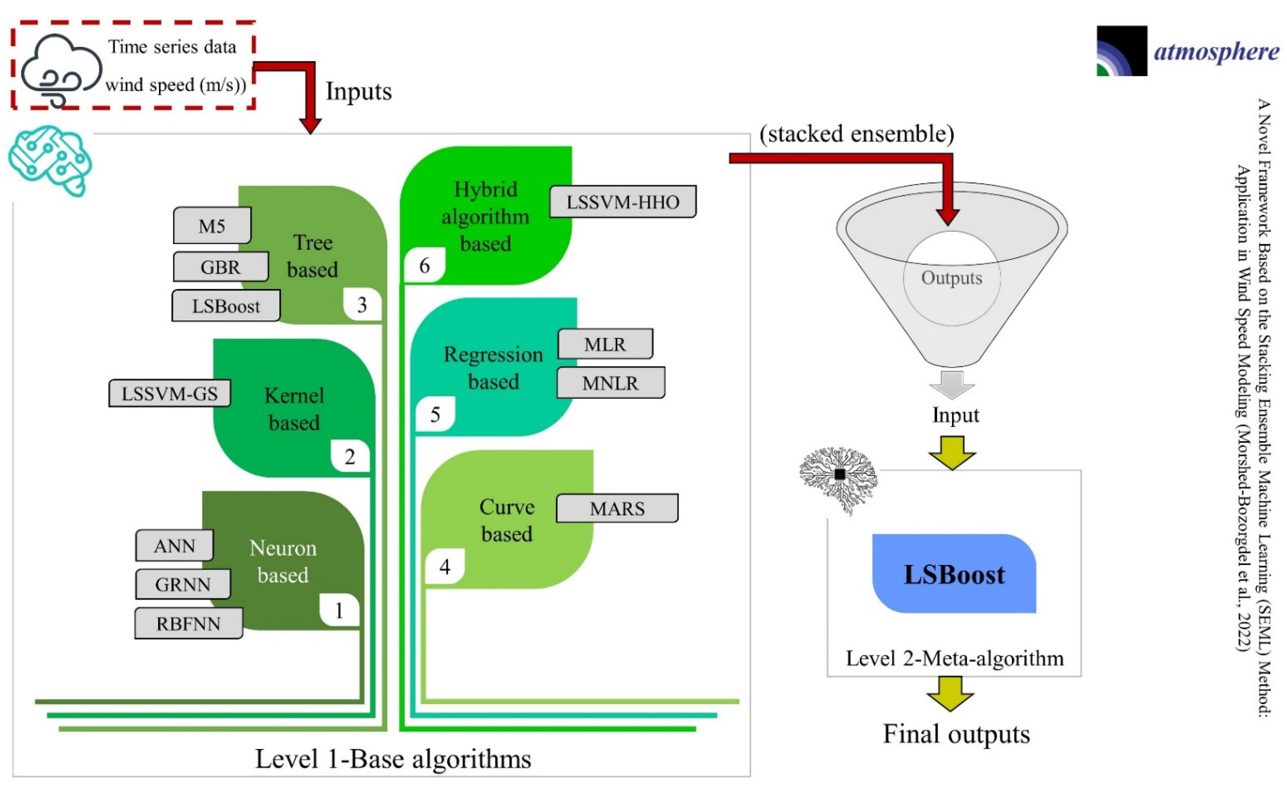
This paper proposes a novel framework for modeling WS. The SEML method combines a wide range of ML algorithms, each of which performs well in a particular field and performs better than any single model in the set. The SEML method works well when several ML algorithms with different properties, structures, and assumptions are used as base algorithms. Base algorithms must be complex and diverse to have different benefits. This novel method allows for the simultaneous use of several algorithms and increases modeling accuracy by using different advantages of algorithms. The pseudo-code of the proposed framework based on the SEML method is described in Algorithm 1. The SEML method consists of two levels:
- Level 1 (base algorithms): All algorithms perform their operations separately at this level. The outputs of this level’s algorithms are used as input into the meta-algorithm.
- Level 2 (meta-algorithm): At this level, the meta-algorithm produces high-precision outputs by combining the results of the level 1 algorithms.
| Algorithm1. Pseudo-code of the proposed framework based on the SEML method. |
|
According to Figure 1, the following steps were performed to model WS using the SEML method:

Figure 1.
Flow chart of the novel framework based on the SEML method for WS modeling.
- Level 1: WS was modeled using eleven ML algorithms, including ANN, MLR, MNLR, GRNN, MARS, M5, GBR, RBFNN, LSBoost, LSSVM-GS, and LSSVM-HHO, at sixteen stations.
- Level 2: Due to the simple structure and high speed of the LSBoost, this algorithm was used as a meta-algorithm to combine the results of the base algorithms.
2.2. Artificial Neural Network (ANN)
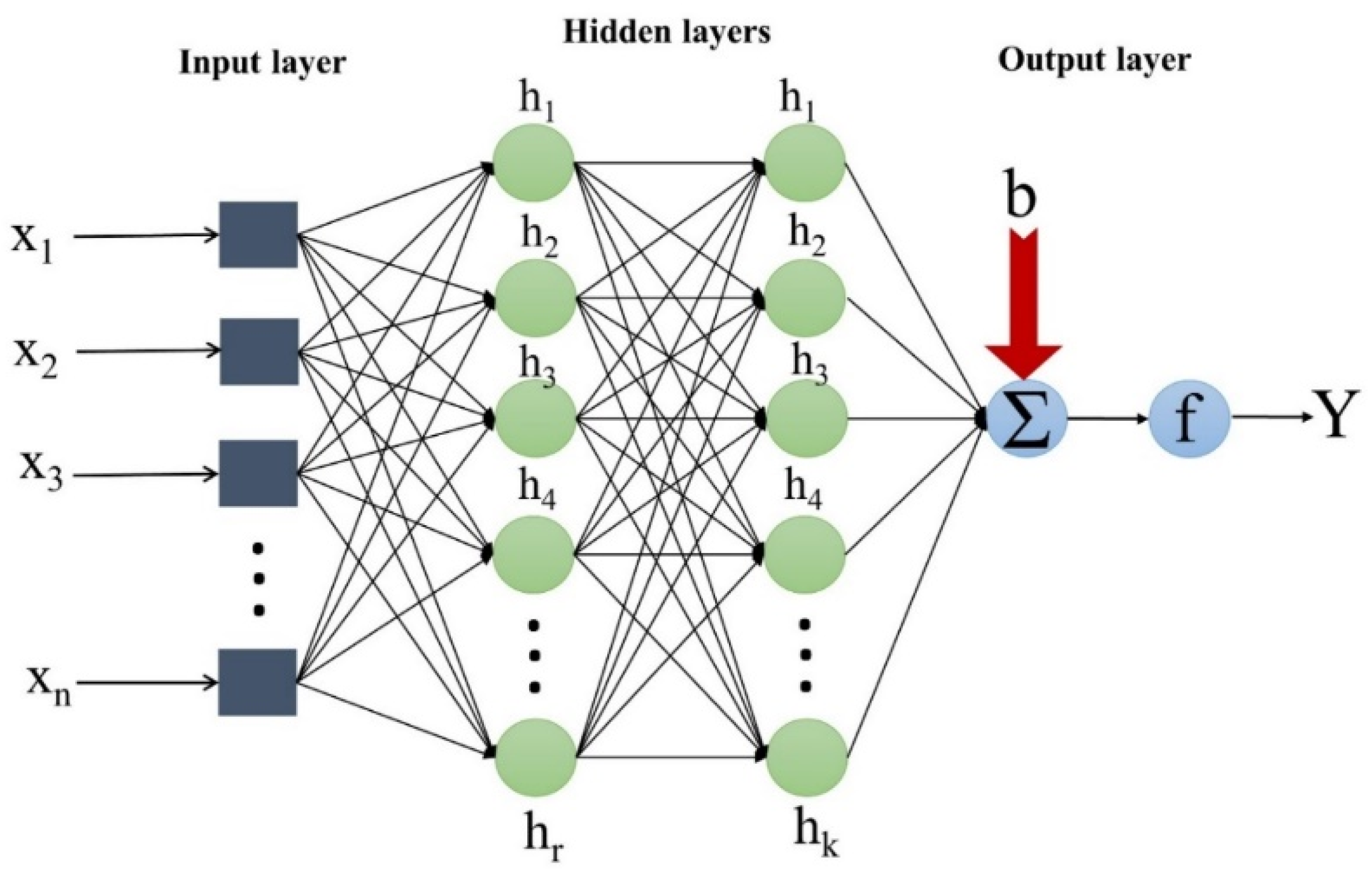
ANN is one of the most popular ML algorithms with a short computational time. It is capable of nonlinear modeling functions [31]. ANN is inspired by a process similar to the human brain to solve various problems. ANN is a data-driven algorithm used to develop the relationship between input and output variables [32]. The ANN comprises different layers (i.e., input, hidden, and output), each containing several neurons (Figure 2). Recently, ANN has been used to model various parameters. In ANN, the relationship between input (x) and output (Y) is as follows:
where g is the stimulation function; b is the bias; is the weight of link.
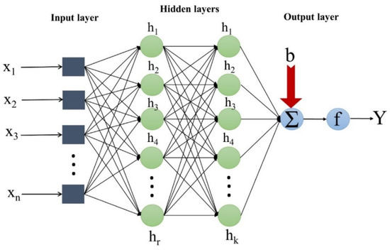
Figure 2.
The schematic structure of ANN.
2.3. Multiple Linear Regression (MLR)
MLR is a statistical method used to model and analyze data [33]. MLR models output data based on a linear relationship [34]. MLR is an extension of ordinary least squares regression because it involves more than one explanatory variable. The MLR is an algorithm for examining the effect of a dependent variable by identifying the relationship of independent variables. The relationship between inputs and goals is assumed to be as follows:
where Y is the dependent variable; x1, x2,…, xn are the independent variables; B1, B2,…, Bn are the coefficients of the independent variables; ε refers to the error term.
2.4. Multiple Nonlinear Regression (MNLR)
The MNLR, unlike the MLR, uses nonlinear regression analysis. In other words, this algorithm estimates the output data by creating a nonlinear combination [35]. The MNLR has more flexibility in modeling high-dimensional data due to the nonlinear relations. The relationship between input and output values in MNLR is as follows:
2.5. General Regression Neural Network (GRNN)
GRNN, obtained from neural network improvement, operates based on nonparametric regression. The GRNN uses the Gaussian kernel regression statistical method to solve various problems [36]. This algorithm does not require an iterative method for data modeling. This ability approximates any desired function between input and output data. The GRNN consists of four layers: input, pattern, summation, and output [37]. The relationship between input (x) and output (Y) in this algorithm is as follows:
where Yi is the weight of the ith neuron connection between the layers; σ is the smoothing factor.
2.6. Multivariate Adaptive Regression Splines (MARS)
The MARS, a nonlinear and nonparametric method, was first proposed by Friedman [38]. This algorithm, which has good performance in solving nonlinear problems with high dimensions, is used to model and predict various parameters. The MARS, which consists of basic functions (BFs), defines nonlinear relationships by determining the weight of input variables. Regression models are determined by combining BFs to estimate the outputs. In this algorithm, BFs depend on spline functions that divide the data set into smaller parts. The structure of this model can be described as follows:
where x is an input; c is a node of the ith BF; Y is an output; wi is the weight of the ith BF; n is the number of BFs; i is the known counter of BF.
2.7. M5 Model Tree (M5)
The M5, a data mining algorithm, was first proposed by Quinlan [39]. The M5 operates in two phases. It first divides the input region into several subsets and uses a specific linear regression model for each subset. Then, a linear regression is established in each node. The structure of the M5 is like a tree growing from the root (first node) to the leaves [40]. Branches are made up of numbers from the initial node to ninety. The growth criterion of the M5 is standard deviation reduction [41]. The random forest estimate is according to specific weights. This algorithm has an acceptable performance due to the random algorithms in a tree formation. The prevailing relation in the M5 is the standard deviation reduction:
where T is a subset of data at each node; Ti is the set of attribute values obtained by dividing T; SD is the standard deviation.
2.8. Gradient Boosted Regression (GBR)
GBR consists of decision trees used for regression and classification tasks [42]. The main structure of GBR is that new models are added to the collection to strengthen the previous model at each stage. This algorithm creates a high-precision prediction model by combining weak models [43]. The advantage of this algorithm is that it can manage lost data. Another advantage of GBR is that it offers several hyper-parameter tuning options, which increases the flexibility of this algorithm. The mathematical formulation of GBR is as follows:
where are the basis functions; are the shrinkage parameters.
2.9. Radial Basis Function Neural Network (RBFNN)
The RBFNN is a feedforward network consisting of three main layers: an input layer, a hidden layer, and an output layer [44]. The input layer is made up of neurons that carry information to the next layer. The hidden layer processes the input information. The nodes in the hidden layer are composed of radial basis functions (RBFs). An RBF is a symmetric function that applies a nonlinear map to input data. The number of hidden layer nodes varies according to the problem under study. The RBFNN uses various hidden layer functions that greatly affect how the algorithm works [45]. The output (Y) of the RBFNN algorithm is as follows:
where wi is the weight of neurons; is the activation function of the RBFNN.
2.10. Least Squares Boost (LSBoost)
The LSBoost, first introduced in 2001 [46], is a deep and group learning method that performs perfectly in modeling and predicting various problems [2]. This algorithm, one of the most advanced gradient amplification algorithms, was developed based on the least squares, absolute, and Huber loss function and is used to increase the accuracy and reduce the variance of the results compared to independent learner samples. This algorithm’s simple structure, high speed, and accuracy are its other advantages. LSBoost uses the following equation to estimate target values:
where is the aggregated prediction for input values ; B1,…, Bm are standalone weak learners; are the weights of the weak learners; is the learning ratio.
2.11. Least Squares Support Vector Machine-Grid Search (LSSVM-GS)
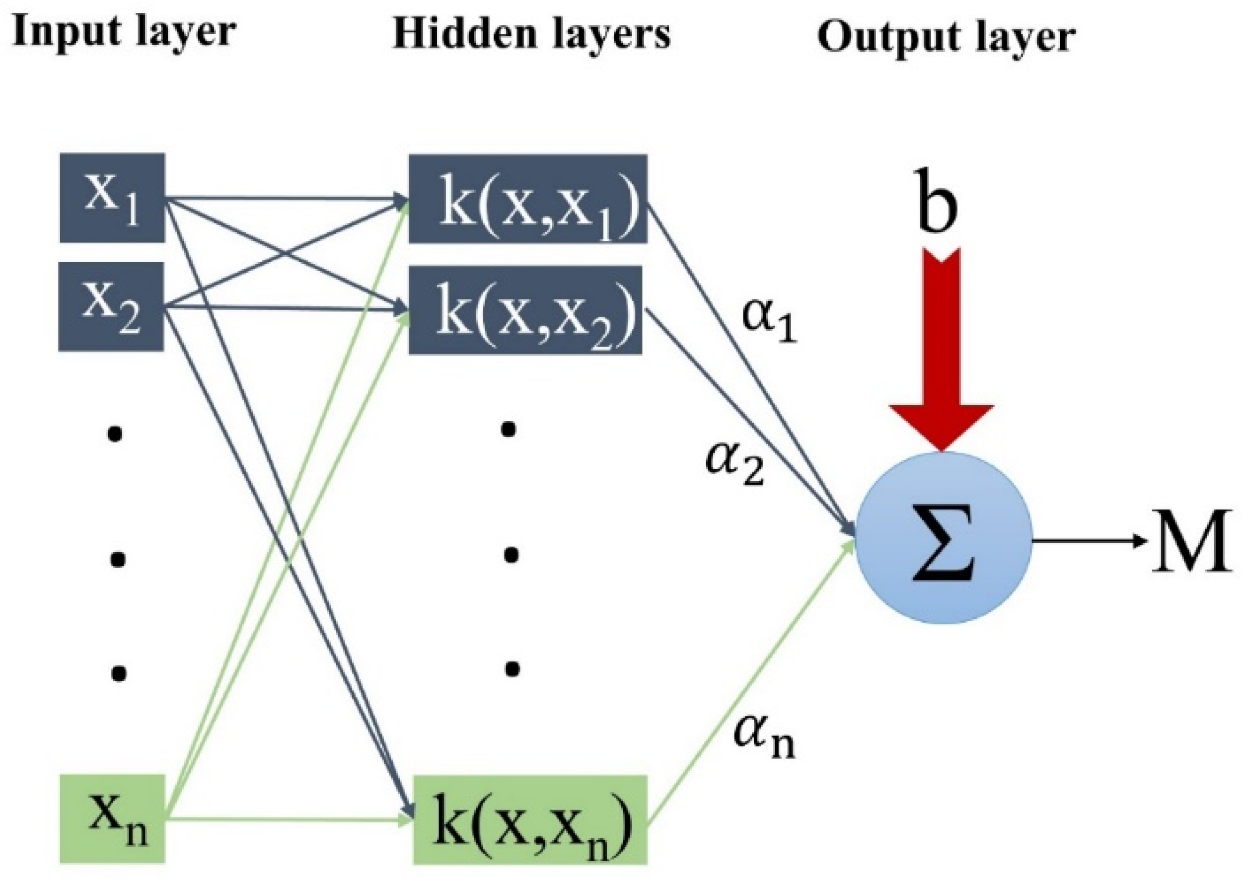
The LSSVM was first proposed by Suykens et al. [47]. The LSSVM is an improved algorithm based on the SVM used for regression analysis, classification, and pattern recognition. This algorithm uses linear relationships instead of nonlinear relationships between inputs (x) and output (M) and significantly improves the accuracy and speed of the SVM. The regression function between input and output in this algorithm is as follows:
where is the ith Lagrange multiplier; K is a kernel function; b is the bias. The parameters and b are computed as follows:
where C is the regulation parameter. The parameters α, M, I, and are computed as follows:
In this paper, the radial basis function was used as a kernel function, which is expressed as follows [48]:
where σ is an effective parameter in the accuracy of the algorithm. The values of C and the core width (σ) have a large effect on the accuracy of the LSSVM. GS can be used to determine the values of these coefficients. GS takes all of the values of C and σ and builds a grid within a certain range. Figure 3 shows the structure of the LSSVM-GS.

Figure 3.
The schematic structure of the LSSVM-GS.
2.12. Harris Hawks Optimization (HHO)
HHO is a population-based algorithm first proposed by Heidari et al. [49]. The performance of this algorithm is inspired by the cooperative behaviors and chasing styles of Harris’ hawks. In this behavior, the Harris’ hawks attack from different directions to surprise the prey. This algorithm has been used in various issues due to the fact of its flexible structure, accuracy, and high speed [50]. For more details, see Heidari et al. [49].
2.13. LSSVM-HHO
Since the C and σ parameters significantly impact how the LSSVM works, it is essential to determine the optimal values of these parameters. Therefore, this study used the HHO optimization algorithm to find the optimal value of the LSSVM parameters. The LSSVM-HHO flow chart is shown in Figure 4. The values, C and σ, are considered decision variables in the hybrid algorithm. In this algorithm, first, training and testing data are randomly selected. Then, the initial parameters of HHO and the initial population of LSSVM are initialized to search for the C and σ values. In the next step, first, the training data are used to obtain the optimal LSSVM. Finally, the testing data are used to evaluate the predictive ability of the LSSVM.
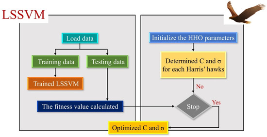
Figure 4.
The schematic structure of the LSSVM-HHO.
2.14. Performance Evaluation of the Algorithms
In the present study, various evaluation criteria, mean absolute error (MAE), root mean squared error (RMSE), relative root mean square error (RRMSE), and R were employed to evaluate the performance of the ML algorithms. The evaluation criteria are given as follows [51,52]:
where N is the number of data; x is the observed values; y is the estimated values; is the mean observed values; is the mean estimated values. The MAE, RMSE, and RRMSE are in the range of zero to infinite positive numbers. The smaller the MAE, RMSE, and RRMSE values, the better the algorithm’s performance. Moreover, the higher the R value, the closer the modeled values are to the actual values, and the best value is one.
2.15. Case Study and Data Sources
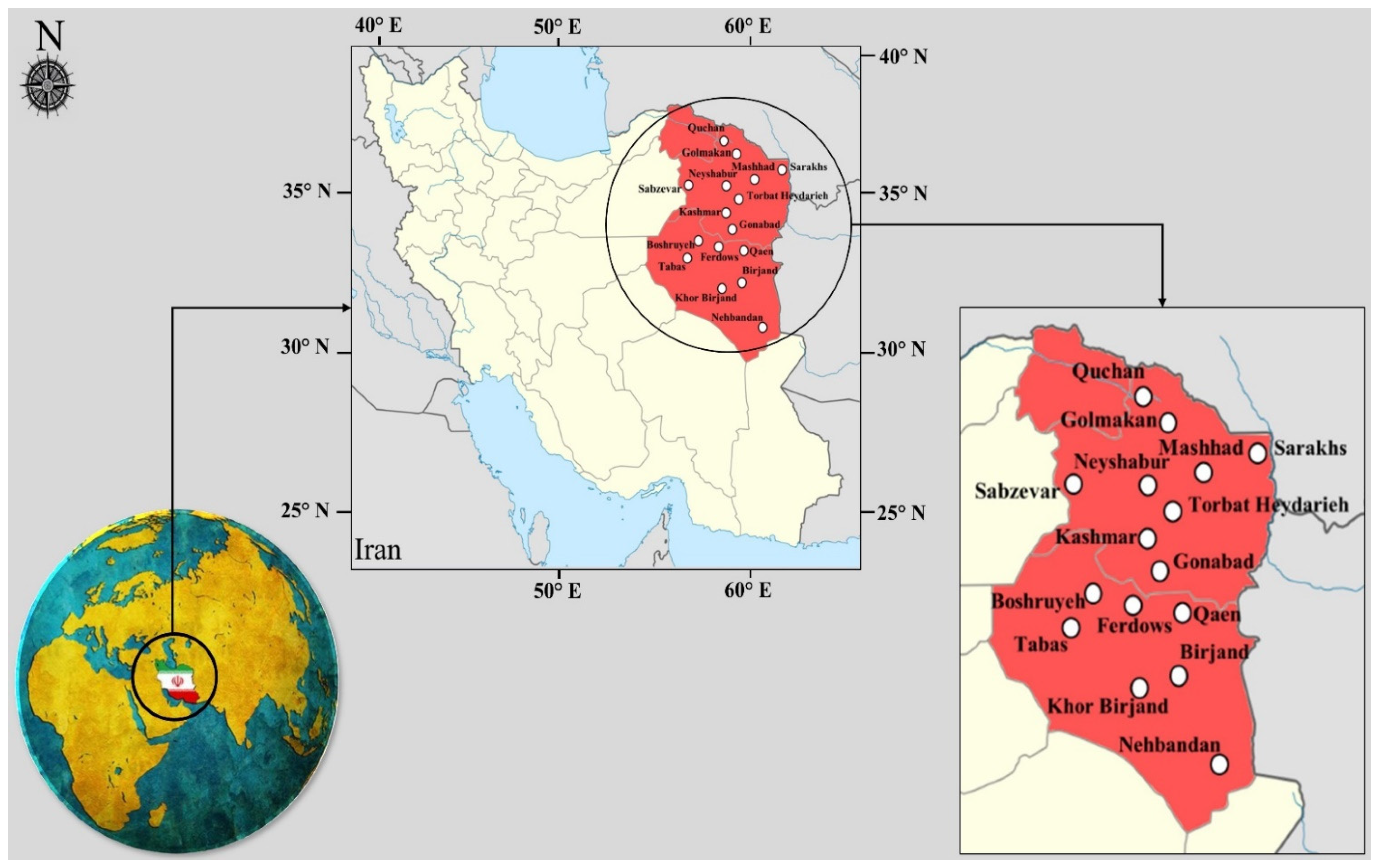
In this study, sixteen synoptic stations located in the east and northeast of Iran were used to model WS and prove the performance of the proposed framework. Nine stations, including Quchan, Sarakhs, Sabzevar, Golmakan, Mashhad, Neyshabur, Torbat Heydarieh, Kashmar, and Gonabad, are located in Khorasan Razavi Province, and seven stations, including Tabas, Ferdows, Qaen, Birjand, Nehbandan, Boshruyeh, and Khor Birjand, are located in South Khorasan Province. The geographical characteristics of the studied stations are stated in Table 1. This region has high potential for the construction of wind farms. Due to the presence of one of the most important wind power plants in Iran in Neyshabur, modeling and predicting WS in this region is very important. In addition, many wind power plants are being built in this area, proving the importance of studied stations. Figure 5 shows the position of the stations used.

Table 1.
Geographic information and statistical specifications of the data from the different stations.

Figure 5.
Case study locations.
The statistical specifications on the data from different stations are given in Table 1. According to Table 1, seven parameters, including minimum air temperature (Tmin), mean air temperature (Tmean), maximum air temperature (Tmax), minimum relative humidity (Hmin), mean relative humidity (Hmean), maximum relative humidity (Hmax), and sunny hours (SH), were used for WS modeling.
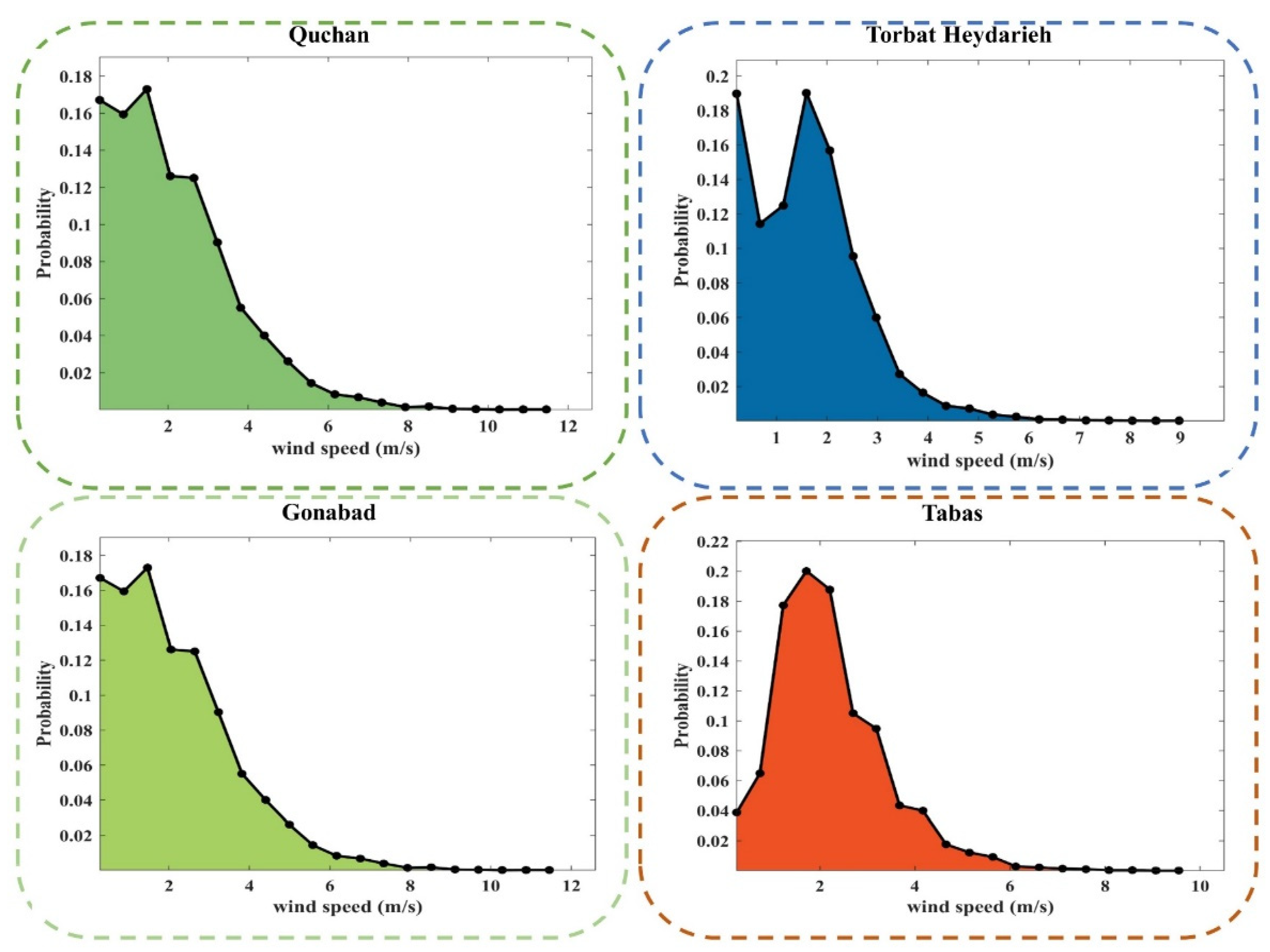
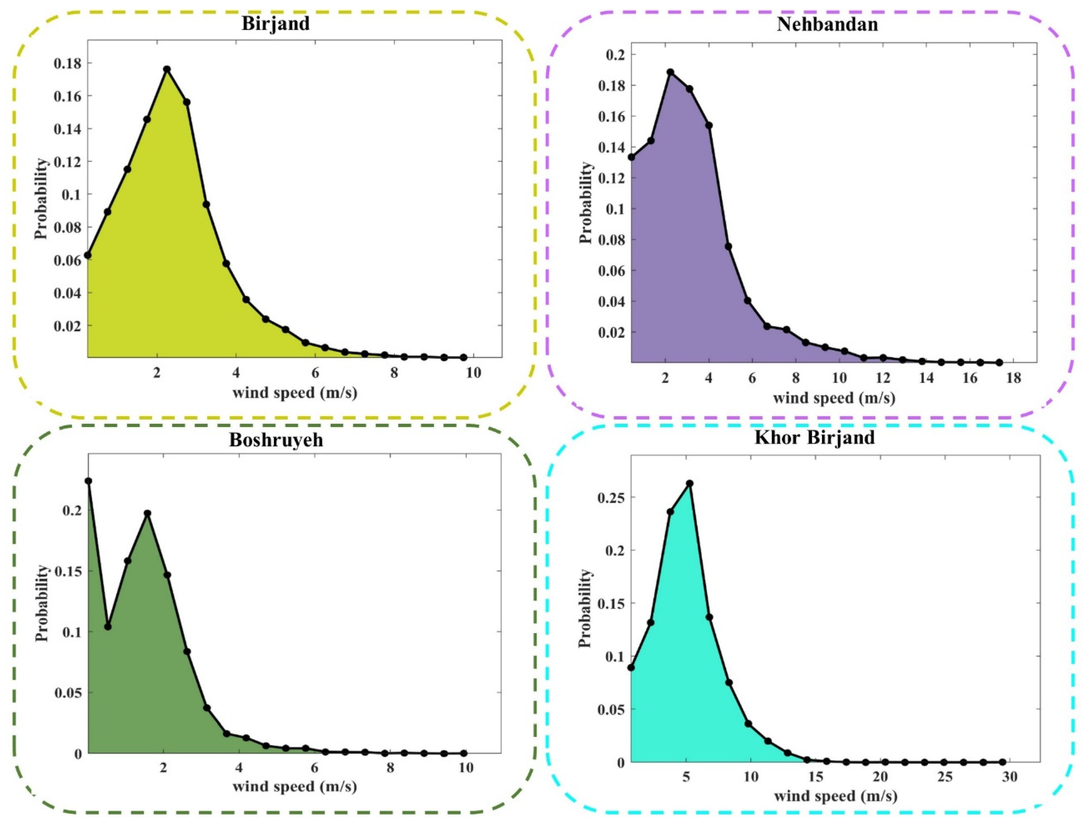
Figure 6 and Figure A1 (Appendix A) show the probability density function (PDF) plot of WS data at the different stations. These figures analyze the volatility of the WS data set in the studied stations. According to these plots, the occurrence probability of any value of WS is calculated. Any WS range that is more likely to occur is known as the prevailing WS of that station.

Figure 6.
PDF plots of the observed values of WS at the different stations.
3. Results and Discussion
3.1. Modeling WS using the SEML Method (Level 1—Base Algorithms)
Because different algorithms have unique features, each of them models only part of the data with good accuracy and does not exhibit good accuracy in other parts of the data. Therefore, using the SEML method combines the capabilities of all algorithms, and the modeling of different parts of the data is performed better. Level 1 of the SEML method aimed to use eleven ML algorithms with different natures and structures and different categories for WS modeling. For this reason, neuron-based, kernel-based, tree-based, curve-based, regression-based, and hybrid algorithm-based algorithms were used in this paper. Table 2, Table A1, Table A2, Table A3, Table A4, Table A5, Table A6, Table A7, Table A8, Table A9, Table A10, Table A11 and Table A12 (Appendix B) state the values of the evaluation criteria for the different algorithms at sixteen stations. According to these tables, the correlation coefficients obtained by the algorithms at all stations ranged from −0.01 to 0.62. This meant the poor performance of ML algorithms in modeling and estimating WS. The large fluctuations of WS values in the studied stations made their modeling difficult. For this reason, the eleven algorithms used in level 1 of the SEML method did not perform well in estimating the target data.

Table 2.
Results of modeling WS with the base algorithms at the different stations.
Table 3 lists the average evaluation criteria obtained by the base algorithms (during the testing period) at sixteen stations. According to this table, the average value of MAE was in the range of 0.96–1.29, the average value of RMSE was in the range of 1.31–1.66, the average value of RRMSE was in the range of 0.84–1.10, and the average value of R was in the range of 0.12–0.51. The average results of WS modeling indicated the low accuracy of the different algorithms. Despite different advantages, the different shortcomings in the structure of the base algorithms led to low modeling accuracy. The proposed framework based on SEML method aimed to eliminate the defects of the base algorithms and increase the modeling accuracy. The SEML method, as an integrated system, combined the results obtained by the level 1 algorithms and applied them to a meta-algorithm. Combining the algorithms’ results meant using all of the features of the base algorithms in WS modeling.

Table 3.
Average results of the algorithms during the testing period at the sixteen stations.
3.2. Modeling WS using the SEML Method (Level 2—Meta-Algorithm)
Due to the poor performance of the ML algorithms in WS modeling, the SEML method was used to increase the accuracy of the algorithms. For this purpose, the LSBoost was used as a meta-algorithm at level 2 of the SEML method. The reason for choosing this algorithm as a meta-algorithm was its simple structure, high accuracy, high speed, and easy execution. At level 2, the outputs obtained by the eleven algorithms were used as the stacked data as the meta-algorithm inputs. Table 4 shows the results of WS modeling by the LSBoost at sixteen stations. As the results show, the average value of MAE was in the range of 0.26–0.71, the average value of RMSE was in the range of 0.44–1.29, the average value of RRMSE was in the range of 0.46–0.60, and the average value of R was in the range of 0.80–0.89. The SEML method increased the WS modeling accuracy by more than 43%. In addition, the values of the other evaluation criteria obtained by the meta-algorithm at the different stations improved the WS data modeling’s accuracy. According to Table 4, the average values of MAE, RMSE, RRMSE, and R in modeling WS at sixteen stations by the meta-algorithm (LSBoost) were 0.43, 0.78, 0.51, and 0.86, respectively. A comparison of the average evaluation criteria obtained by the LSBoost in Table 3 and Table 4 showed the effect of the SEML method on improving the accuracy of WS modeling. Simultaneous use of the advantages of different algorithms at level 2 of the SEML method by LSBoost led to a significant increase in modeling accuracy. In addition, using different categories in the base algorithms led to using the advantages and features of the different algorithms in this framework. This eliminated the shortcomings of the algorithms in the proposed framework. According to the modeling results with LSBoost, the highest modeling accuracies were obtained at Quchan station (MAE = 0.41, RMSE = 0.71, RRMSE = 0.46, and R = 0.89) and Neyshabur station (MAE = 0.26, RMSE = 0.44, RRMSE = 0.49, and R = 0.87).

Table 4.
Results of modeling WS with LSBoost (meta-algorithm) at the different stations.
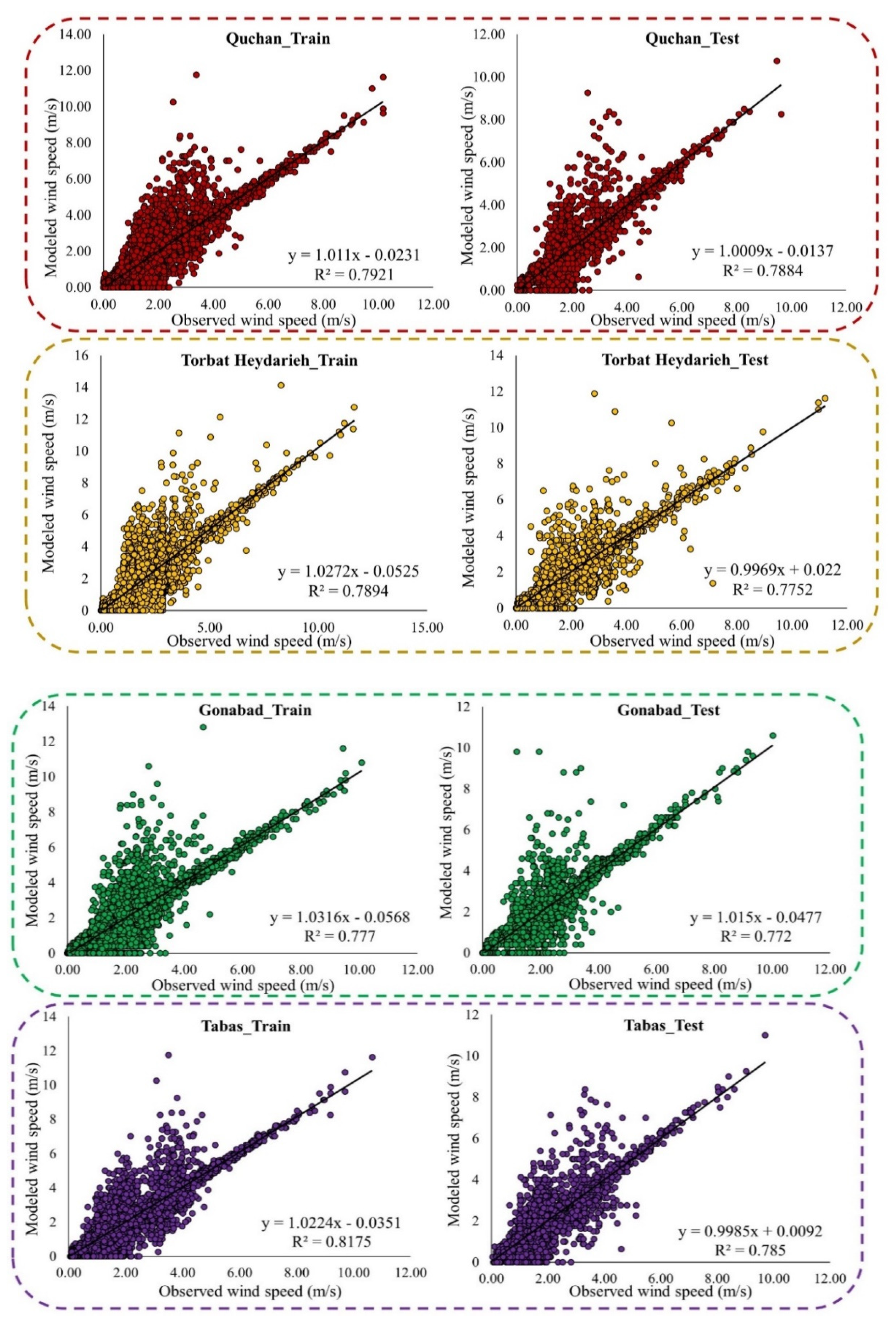
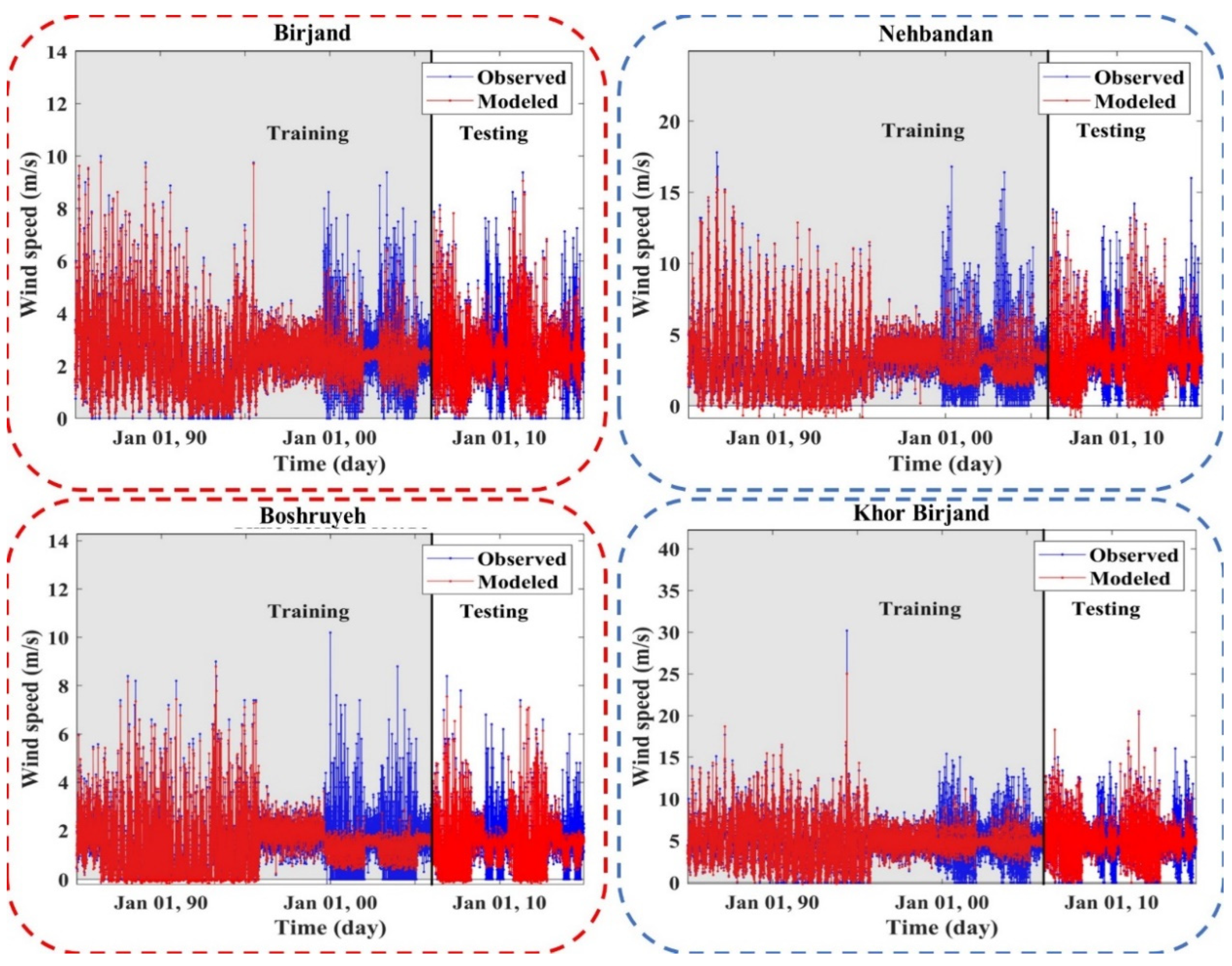
Figure 7, Figure 8, Figure A2 and Figure A3 (Appendix C) show the results of the scatter plot and time series of the observed data and the data modeled by the LSBoost. It is clear from these figures that the proposed novel framework successfully performed WS modeling. In addition, the use of the SEML method in WS modeling significantly increased the accuracy of the algorithms, so that the values of the evaluation criteria in level 2 were improved compared to the base algorithms at all stations. According to the scatterplots, the difference between the values modeled by the meta-algorithm and the observed values was very small. Since most of the modeled and observed values were collected around the semiconductor line, the accuracy of the LSBoost in WS modeling was high. Moreover, according to the time series diagrams, the data model at level 2 of the SEML method was largely matched to the observed data. Accurate estimations of the maximum and minimum WS values by meta-algorithm show the simultaneous use of the advantages of base algorithms and their application in level 2 of the SEML method.

Figure 7.
Scatter plots of the observed and modeled values of WS using the meta-algorithm at different stations.
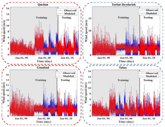
Figure 8.
Time series of the observed and modeled values of WS using the meta-algorithm at different stations.
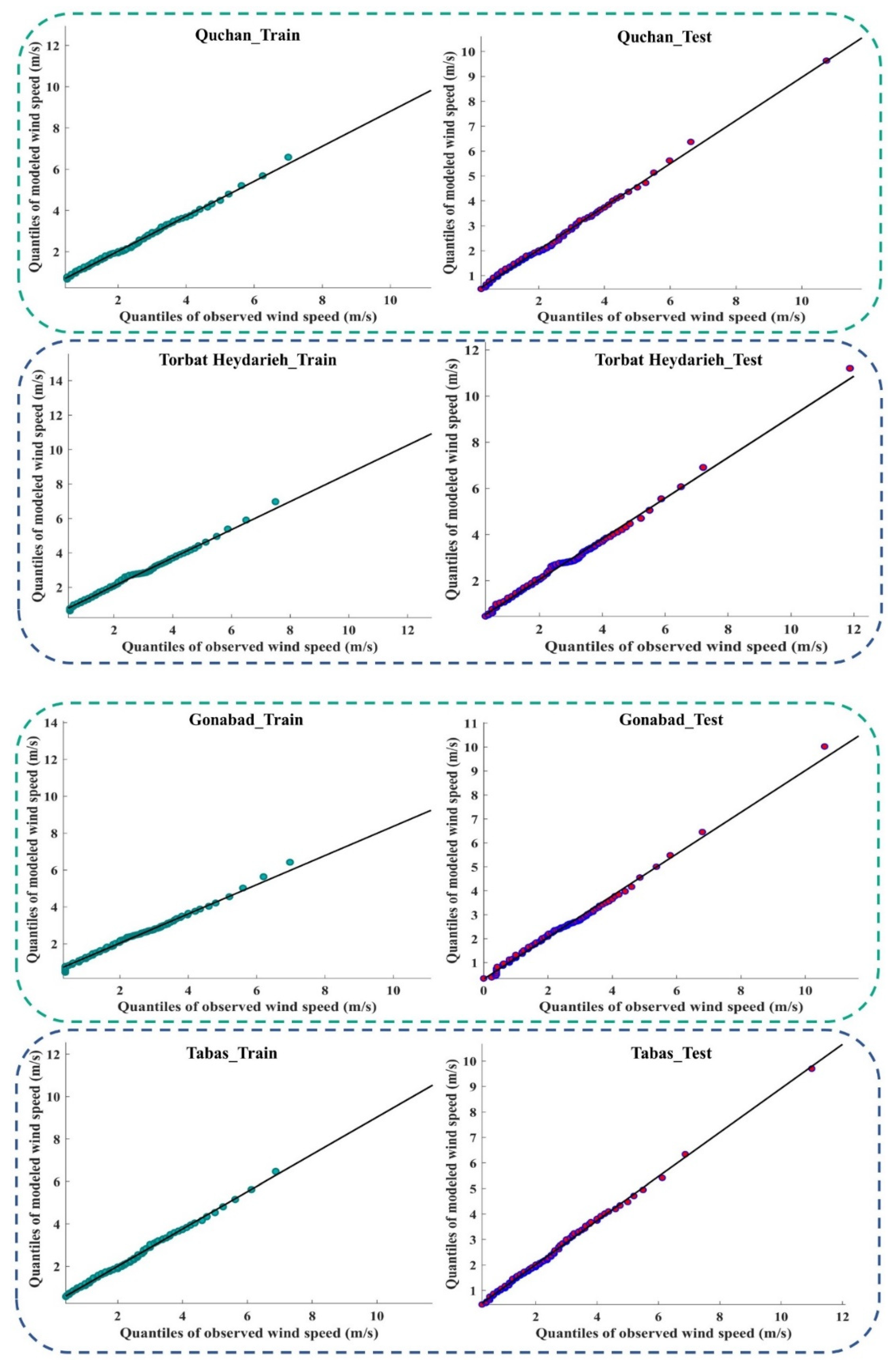
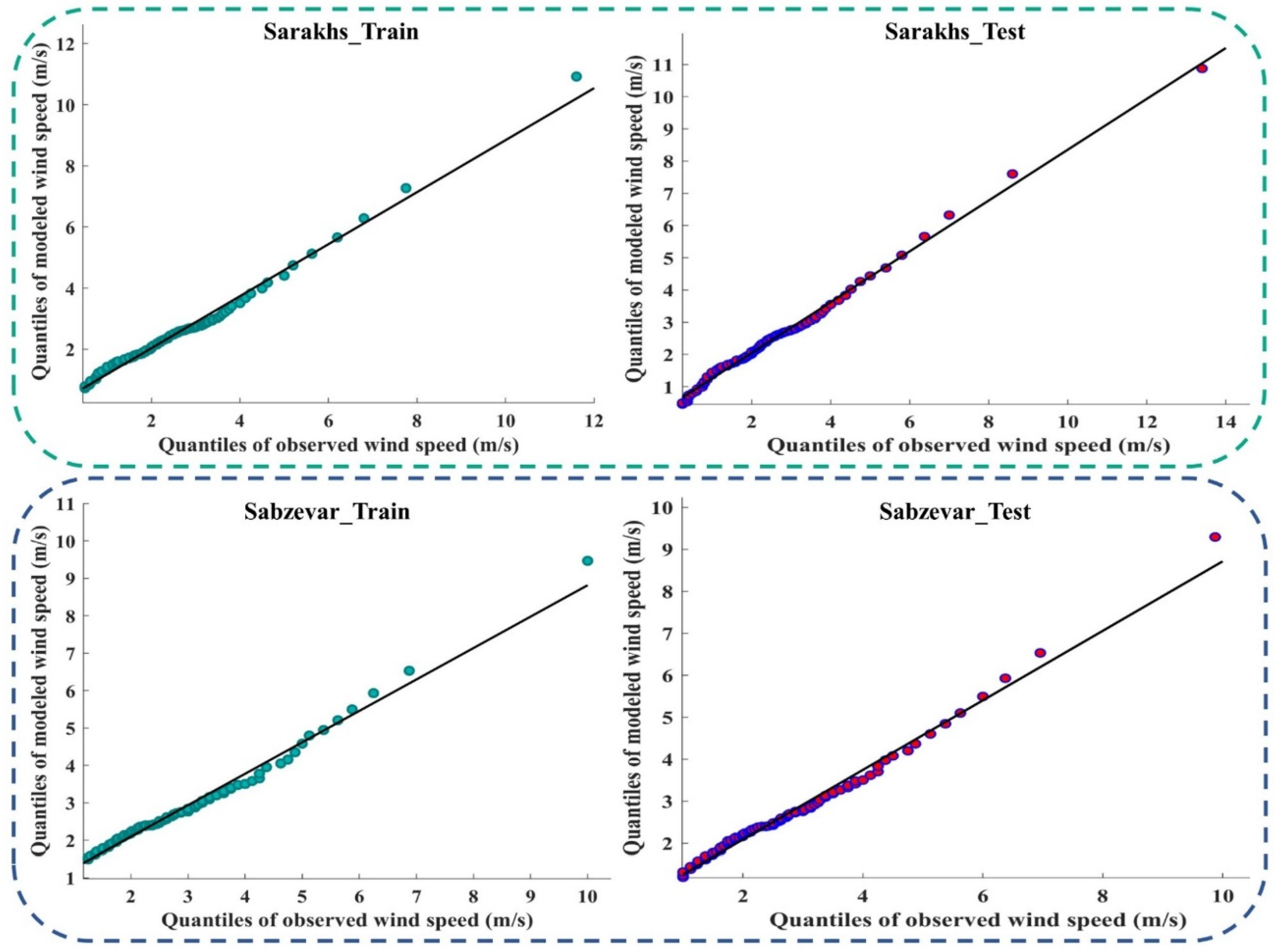
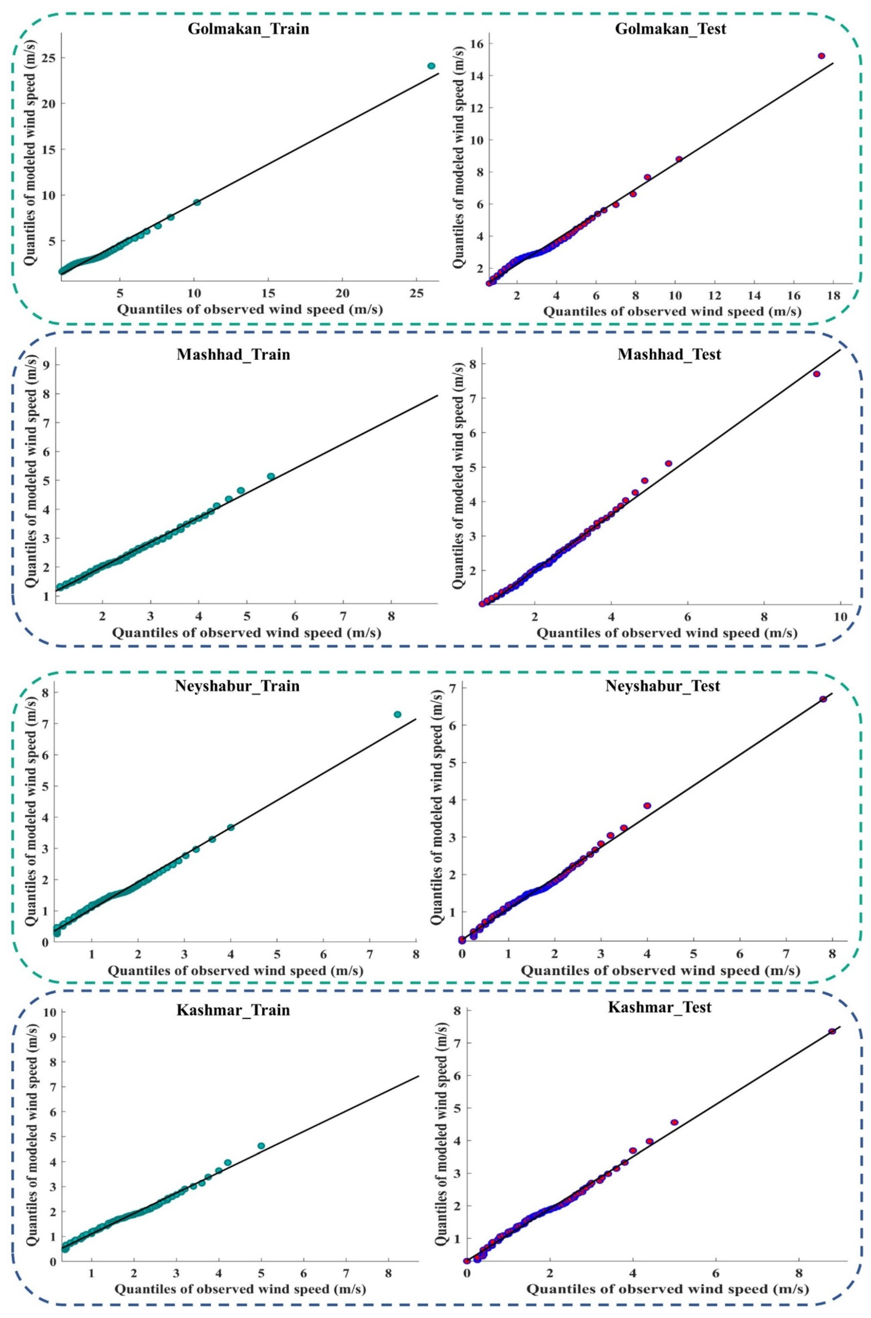
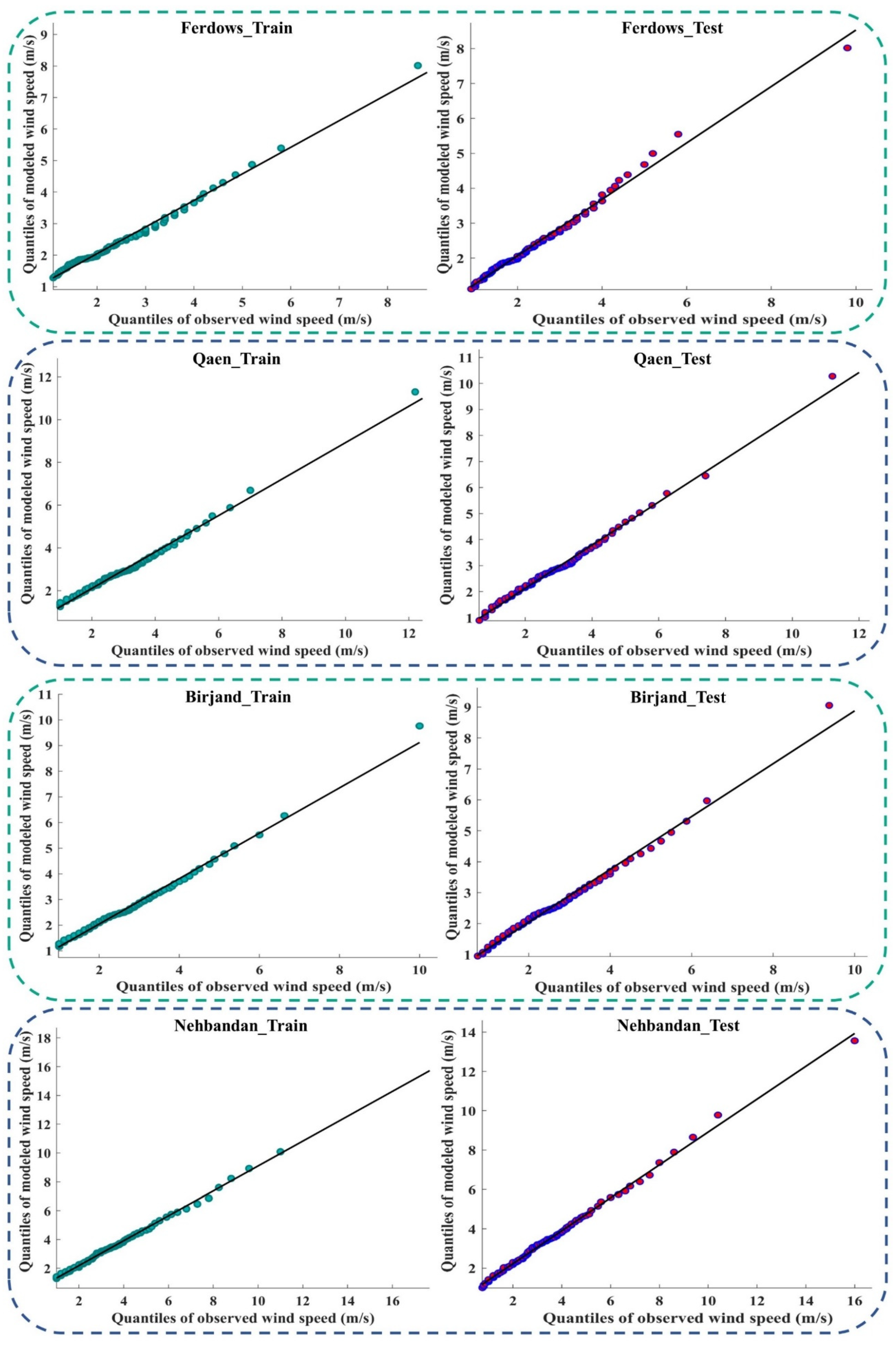
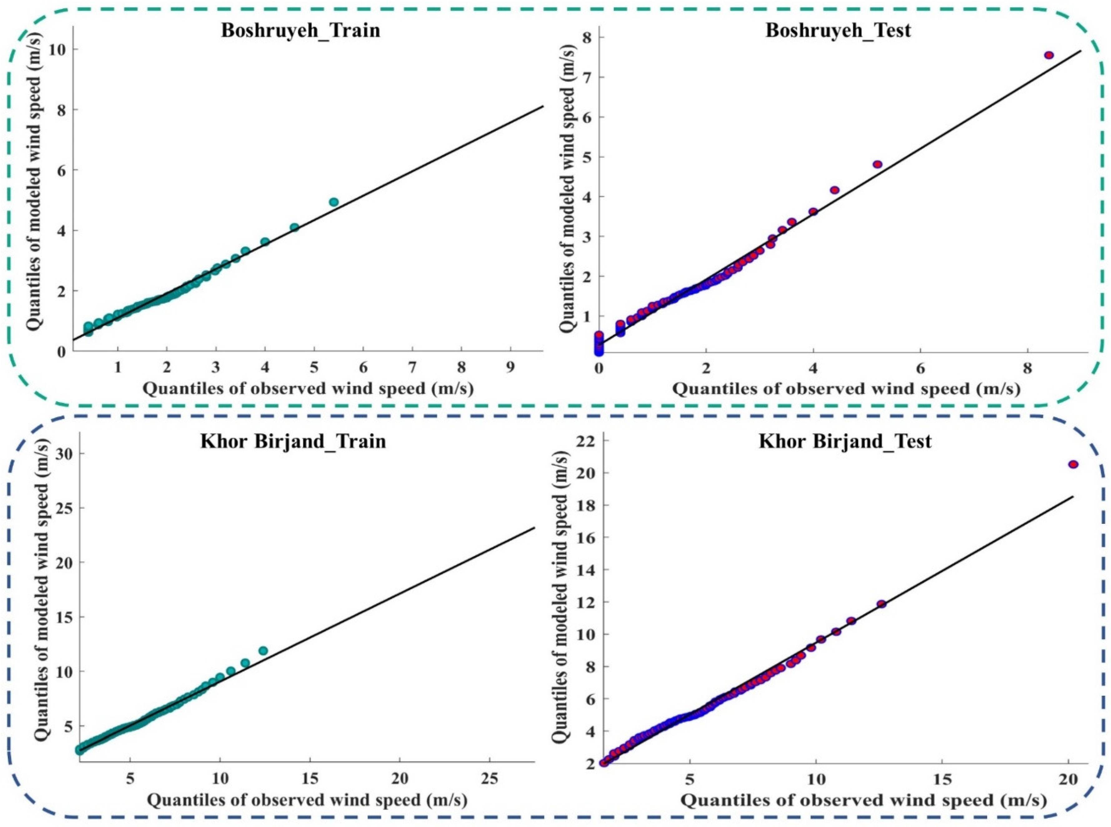
Figure 9 and Figure A4 (Appendix D) show the quantile–quantile plot (Q–Q plot) at different stations. In these plots, the probability distributions of the observed data were plotted against the probability distributions of the data modeled by the meta-algorithm (LSBoost). The more points collected around line 45°, the more equal the probabilistic distributions of the observed and modeled data. The accumulation of points around the 45° line also showed a slight difference between the observed and modeled data. According to the descriptions provided during the test period, the observed and modeled data had an equal distribution at most stations. This means that the LSBoost in the structure of the SEML method modeled the WS data with high accuracy.

Figure 9.
Q–Q plots of observed and modeled values of WS using the meta-algorithm at different stations.
4. Conclusions
Accurate and reliable modeling and predicting WS is critical to planning and managing power generation. WS modeling was performed at sixteen stations in Iran at two levels to achieve this goal. In level 1 of this method, eleven ML algorithms, including ANN, MLR, MNLR, GRNN, MARS, M5, GBR, RBFNN, LSBoost, LSSVM-GS, and LSSVM-HHO, in six categories (neuron based, kernel based, tree based, curve based, regression based, and hybrid algorithm based) were used as base algorithms. In level 2, the outputs of the base algorithms were applied as input to the meta-algorithm (LSBoost). Thus, the final results of WS modeling were obtained. Applying the results of the base algorithms to the LSBoost at level 2 of the SEML method increased the modeling accuracy by >43%. Improving the evaluation criteria at all stations proved the strength of the novel framework. The average values of MAE, RMSE, RRMSE, and R in modeling WS at sixteen stations using the meta-algorithm (LSBoost) were 0.43, 0.78, 0.51, and 0.86, respectively. According to the results of this study, the proposed framework has high potential for analysis of other engineering issues and meteorological parameters. This framework can improve the performance of ML algorithms in modeling and predicting WS in areas where ML algorithms perform poorly. Moreover, using this novel framework, WS can be predicted in different basins and the optimal use of WS and electricity generation can be planned. The performance of the proposed framework can be improved by using appropriate algorithms and various techniques such as wavelet transform. As a result, we achieved the desired goal of providing a novel framework based on the SEML method.
Author Contributions
Conceptualization, S.F.; Data curation, A.M.-B., M.K. and M.V.A.; Formal analysis, A.M.-B., M.K., M.V.A. and S.F.; Investigation, A.M.-B., M.K. and S.F.; Methodology, A.M.-B., M.K. and M.V.A.; Project administration, S.F.; Resources, S.F. and M.V.A.; Software, A.M.-B., M.K. and M.V.A.; Supervision, S.F.; Validation, A.M.-B., M.K. and M.V.A.; Visualization, A.M.-B., M.K. and M.V.A.; Writing—original draft, A.M.-B. and M.K.; Writing—review and editing, S.F. and M.V.A. All authors have read and agreed to the published version of the manuscript.
Funding
This research was not supported through any funds.
Institutional Review Board Statement
Not applicable.
Informed Consent Statement
Not applicable.
Data Availability Statement
All data generated or used during the study are applicable if requested.
Conflicts of Interest
The authors declare that they have no conflict of interest.
Appendix A

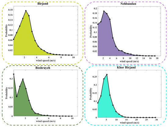
Figure A1.
PDF plots of observed values of WS at different stations.
Figure A1.
PDF plots of observed values of WS at different stations.
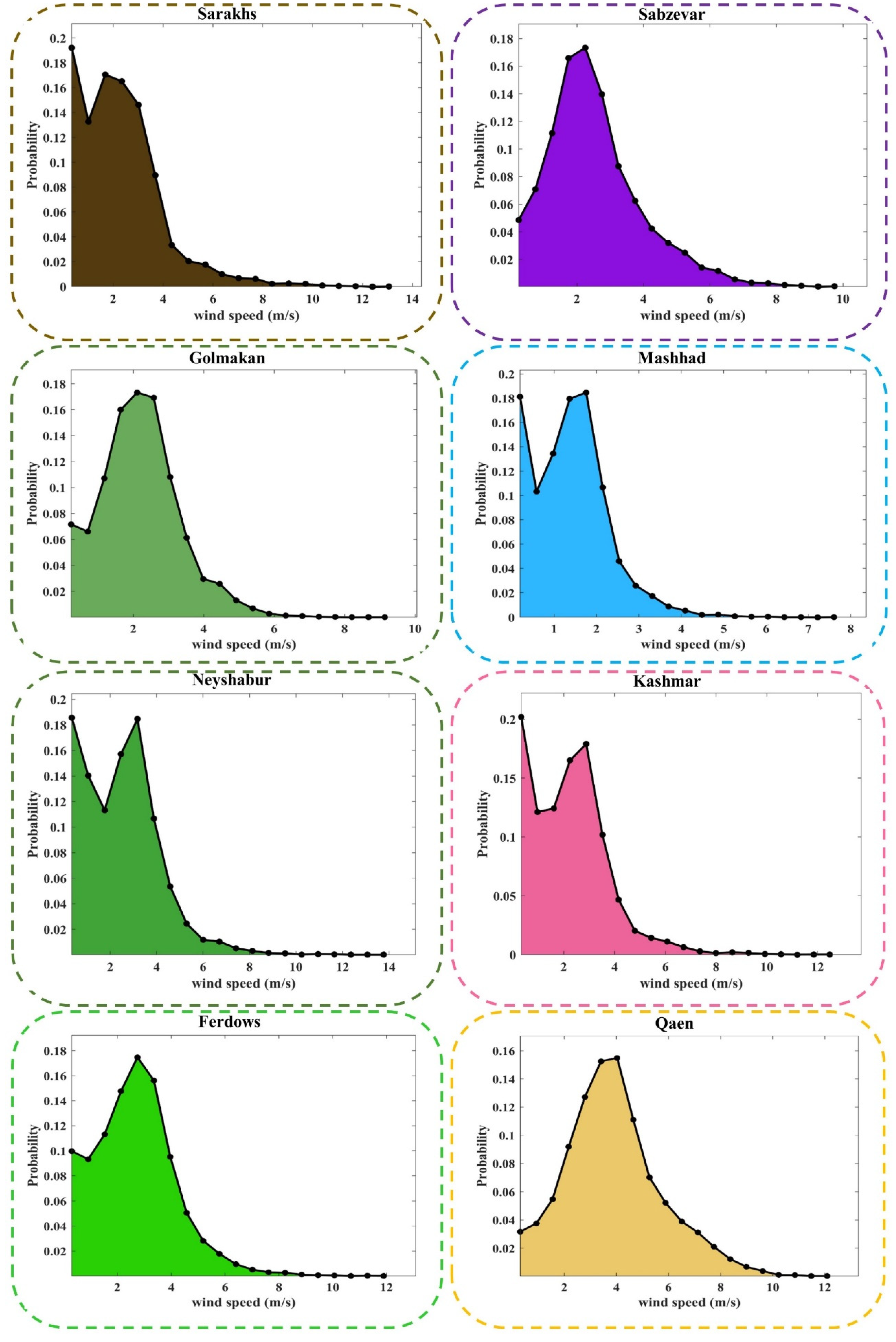
Appendix B

Table A1.
Results of modeling WS with the base algorithms at the Sarakhs station.
Table A1.
Results of modeling WS with the base algorithms at the Sarakhs station.
| Training | Testing | |||||||
|---|---|---|---|---|---|---|---|---|
| MAE | RMSE | RRMSE | R | MAE | RMSE | RRMSE | R | |
| ANN | 1.10 | 1.50 | 0.89 | 0.46 | 1.11 | 1.52 | 0.91 | 0.42 |
| MLR | 1.18 | 1.58 | 0.94 | 0.34 | 1.17 | 1.58 | 0.95 | 0.32 |
| MNLR | 1.16 | 1.56 | 0.93 | 0.37 | 1.15 | 1.56 | 0.94 | 0.35 |
| GRNN | 0.86 | 1.21 | 0.72 | 0.74 | 1.13 | 1.56 | 0.93 | 0.36 |
| MARS | 1.14 | 1.54 | 0.91 | 0.41 | 1.13 | 1.54 | 0.92 | 0.40 |
| M5 | 1.13 | 1.53 | 0.91 | 0.41 | 1.13 | 1.56 | 0.93 | 0.37 |
| GBR | 1.03 | 1.39 | 0.83 | 0.59 | 1.11 | 1.52 | 0.91 | 0.42 |
| RBFNN | 0.00 | 0.00 | 0.00 | 1.00 | 1.43 | 1.81 | 1.08 | −0.01 |
| LSBoost | 1.06 | 1.41 | 0.84 | 0.57 | 1.12 | 1.54 | 0.92 | 0.40 |
| LSSVM-GS | 0.95 | 1.28 | 0.76 | 0.68 | 1.11 | 1.52 | 0.91 | 0.42 |
| LSSVM-HHO | 1.03 | 1.39 | 0.82 | 0.59 | 1.11 | 1.52 | 0.91 | 0.42 |

Table A2.
Results of modeling WS with the base algorithms at the Sabzevar station.
Table A2.
Results of modeling WS with the base algorithms at the Sabzevar station.
| Training | Testing | |||||||
|---|---|---|---|---|---|---|---|---|
| MAE | RMSE | RRMSE | R | MAE | RMSE | RRMSE | R | |
| ANN | 0.92 | 1.23 | 0.86 | 0.51 | 0.98 | 1.29 | 0.88 | 0.47 |
| MLR | 0.93 | 1.25 | 0.87 | 0.49 | 0.98 | 1.30 | 0.89 | 0.46 |
| MNLR | 0.93 | 1.24 | 0.86 | 0.50 | 0.98 | 1.29 | 0.88 | 0.47 |
| GRNN | 0.69 | 0.97 | 0.68 | 0.75 | 0.98 | 1.30 | 0.89 | 0.47 |
| MARS | 0.92 | 1.23 | 0.86 | 0.51 | 0.98 | 1.29 | 0.88 | 0.47 |
| M5 | 0.91 | 1.22 | 0.85 | 0.53 | 0.99 | 1.30 | 0.89 | 0.46 |
| GBR | 0.78 | 1.05 | 0.73 | 0.70 | 0.97 | 1.28 | 0.87 | 0.49 |
| RBFNN | 0.00 | 0.00 | 0.00 | 1.00 | 1.71 | 1.95 | 1.33 | 0.00 |
| LSBoost | 0.89 | 1.18 | 0.83 | 0.57 | 0.97 | 1.29 | 0.88 | 0.48 |
| LSSVM-GS | 0.78 | 1.04 | 0.73 | 0.70 | 0.97 | 1.28 | 0.87 | 0.49 |
| LSSVM-HHO | 0.78 | 1.05 | 0.73 | 0.70 | 0.97 | 1.28 | 0.87 | 0.49 |

Table A3.
Results of modeling WS with the base algorithms in the Golmakan station.
Table A3.
Results of modeling WS with the base algorithms in the Golmakan station.
| Training | Testing | |||||||
|---|---|---|---|---|---|---|---|---|
| MAE | RMSE | RRMSE | R | MAE | RMSE | RRMSE | R | |
| ANN | 1.35 | 1.92 | 0.97 | 0.25 | 1.45 | 2.07 | 0.98 | 0.20 |
| MLR | 1.38 | 1.96 | 0.99 | 0.16 | 1.46 | 2.08 | 0.99 | 0.17 |
| MNLR | 1.37 | 1.95 | 0.98 | 0.19 | 1.45 | 2.07 | 0.98 | 0.18 |
| GRNN | 0.99 | 1.44 | 0.73 | 0.75 | 1.48 | 2.12 | 1.01 | 0.11 |
| MARS | 1.37 | 1.94 | 0.98 | 0.21 | 1.45 | 2.07 | 0.98 | 0.19 |
| M5 | 1.35 | 1.92 | 0.97 | 0.25 | 1.47 | 2.09 | 0.99 | 0.16 |
| GBR | 1.29 | 1.84 | 0.93 | 0.43 | 1.45 | 2.07 | 0.98 | 0.20 |
| RBFNN | 0.00 | 0.00 | 0.00 | 1.00 | 1.48 | 2.11 | 1.00 | 0.01 |
| LSBoost | 1.33 | 1.88 | 0.95 | 0.35 | 1.45 | 2.07 | 0.98 | 0.18 |
| LSSVM-GS | 1.15 | 1.63 | 0.82 | 0.69 | 1.45 | 2.07 | 0.98 | 0.19 |
| LSSVM-HHO | 1.29 | 1.84 | 0.93 | 0.43 | 1.45 | 2.07 | 0.98 | 0.20 |

Table A4.
Results of modeling WS with the base algorithms at the Mashhad station.
Table A4.
Results of modeling WS with the base algorithms at the Mashhad station.
| Training | Testing | |||||||
|---|---|---|---|---|---|---|---|---|
| MAE | RMSE | RRMSE | R | MAE | RMSE | RRMSE | R | |
| ANN | 0.77 | 1.02 | 0.87 | 0.49 | 0.80 | 1.04 | 0.89 | 0.46 |
| MLR | 0.79 | 1.05 | 0.90 | 0.43 | 0.81 | 1.06 | 0.91 | 0.42 |
| MNLR | 0.79 | 1.05 | 0.90 | 0.44 | 0.81 | 1.06 | 0.90 | 0.43 |
| GRNN | 0.58 | 0.79 | 0.67 | 0.77 | 0.80 | 1.07 | 0.91 | 0.42 |
| MARS | 0.79 | 1.04 | 0.89 | 0.45 | 0.81 | 1.05 | 0.90 | 0.43 |
| M5 | 0.78 | 1.04 | 0.89 | 0.45 | 0.81 | 1.07 | 0.91 | 0.41 |
| GBR | 0.72 | 0.95 | 0.82 | 0.59 | 0.80 | 1.05 | 0.89 | 0.45 |
| RBFNN | 0.00 | 0.00 | 0.00 | 1.00 | 2.20 | 2.49 | 2.13 | 0.00 |
| LSBoost | 0.76 | 1.00 | 0.86 | 0.52 | 0.80 | 1.05 | 0.90 | 0.44 |
| LSSVM-GS | 0.66 | 0.87 | 0.75 | 0.69 | 0.80 | 1.05 | 0.90 | 0.44 |
| LSSVM-HHO | 0.72 | 0.95 | 0.82 | 0.59 | 0.80 | 1.05 | 0.89 | 0.45 |

Table A5.
Results of modeling WS with the base algorithms at the Neyshabur station.
Table A5.
Results of modeling WS with the base algorithms at the Neyshabur station.
| Training | Testing | |||||||
|---|---|---|---|---|---|---|---|---|
| MAE | RMSE | RRMSE | R | MAE | RMSE | RRMSE | R | |
| ANN | 0.59 | 0.79 | 0.86 | 0.51 | 0.59 | 0.80 | 0.88 | 0.48 |
| MLR | 0.61 | 0.81 | 0.89 | 0.46 | 0.61 | 0.82 | 0.90 | 0.44 |
| MNLR | 0.60 | 0.80 | 0.88 | 0.47 | 0.61 | 0.81 | 0.89 | 0.45 |
| GRNN | 0.45 | 0.63 | 0.70 | 0.74 | 0.61 | 0.82 | 0.90 | 0.44 |
| MARS | 0.59 | 0.79 | 0.87 | 0.50 | 0.59 | 0.80 | 0.88 | 0.48 |
| M5 | 0.59 | 0.79 | 0.87 | 0.49 | 0.60 | 0.81 | 0.89 | 0.46 |
| GBR | 0.51 | 0.69 | 0.76 | 0.67 | 0.59 | 0.79 | 0.87 | 0.49 |
| RBFNN | 0.00 | 0.00 | 0.00 | 1.00 | 0.71 | 0.91 | 1.00 | 0.00 |
| LSBoost | 0.57 | 0.76 | 0.83 | 0.56 | 0.60 | 0.80 | 0.88 | 0.47 |
| LSSVM-GS | 0.50 | 0.67 | 0.74 | 0.70 | 0.59 | 0.79 | 0.87 | 0.49 |
| LSSVM-HHO | 0.51 | 0.69 | 0.76 | 0.67 | 0.59 | 0.79 | 0.87 | 0.49 |

Table A6.
Results of modeling WS with the base algorithms at the Kashmar station.
Table A6.
Results of modeling WS with the base algorithms at the Kashmar station.
| Training | Testing | |||||||
|---|---|---|---|---|---|---|---|---|
| MAE | RMSE | RRMSE | R | MAE | RMSE | RRMSE | R | |
| ANN | 0.75 | 1.01 | 0.91 | 0.42 | 0.75 | 1.01 | 0.90 | 0.45 |
| MLR | 0.77 | 1.04 | 0.93 | 0.37 | 0.76 | 1.03 | 0.91 | 0.41 |
| MNLR | 0.77 | 1.03 | 0.92 | 0.38 | 0.76 | 1.03 | 0.91 | 0.42 |
| GRNN | 0.58 | 0.81 | 0.72 | 0.72 | 0.77 | 1.04 | 0.92 | 0.39 |
| MARS | 0.75 | 1.02 | 0.91 | 0.41 | 0.75 | 1.02 | 0.90 | 0.44 |
| M5 | 0.75 | 1.02 | 0.91 | 0.41 | 0.75 | 1.02 | 0.90 | 0.44 |
| GBR | 0.68 | 0.93 | 0.83 | 0.58 | 0.75 | 1.01 | 0.90 | 0.45 |
| RBFNN | 0.00 | 0.00 | 0.00 | 1.00 | 0.84 | 1.11 | 0.98 | 0.22 |
| LSBoost | 0.71 | 0.95 | 0.85 | 0.54 | 0.75 | 1.02 | 0.90 | 0.43 |
| LSSVM-GS | 0.64 | 0.87 | 0.78 | 0.67 | 0.75 | 1.02 | 0.90 | 0.44 |
| LSSVM-HHO | 0.64 | 0.87 | 0.78 | 0.67 | 0.75 | 1.02 | 0.90 | 0.44 |

Table A7.
Results of modeling WS with the base algorithms at the Ferdows station.
Table A7.
Results of modeling WS with the base algorithms at the Ferdows station.
| Training | Testing | |||||||
|---|---|---|---|---|---|---|---|---|
| MAE | RMSE | RRMSE | R | MAE | RMSE | RRMSE | R | |
| ANN | 0.77 | 1.03 | 0.88 | 0.47 | 0.80 | 1.08 | 0.90 | 0.44 |
| MLR | 0.79 | 1.07 | 0.91 | 0.42 | 0.81 | 1.09 | 0.91 | 0.41 |
| MNLR | 0.79 | 1.06 | 0.90 | 0.43 | 0.81 | 1.09 | 0.91 | 0.42 |
| GRNN | 0.57 | 0.80 | 0.68 | 0.76 | 0.81 | 1.10 | 0.92 | 0.40 |
| MARS | 0.79 | 1.05 | 0.90 | 0.44 | 0.80 | 1.08 | 0.90 | 0.43 |
| M5 | 0.78 | 1.05 | 0.89 | 0.46 | 0.82 | 1.11 | 0.92 | 0.39 |
| GBR | 0.72 | 0.97 | 0.82 | 0.58 | 0.80 | 1.07 | 0.90 | 0.44 |
| RBFNN | 0.00 | 0.00 | 0.00 | 1.00 | 0.94 | 1.21 | 1.01 | 0.03 |
| LSBoost | 0.73 | 0.97 | 0.83 | 0.58 | 0.80 | 1.08 | 0.90 | 0.43 |
| LSSVM-GS | 0.66 | 0.89 | 0.76 | 0.69 | 0.80 | 1.07 | 0.90 | 0.44 |
| LSSVM-HHO | 0.72 | 0.97 | 0.82 | 0.58 | 0.80 | 1.07 | 0.90 | 0.44 |

Table A8.
Results of modeling WS with the base algorithms at the Qaen station.
Table A8.
Results of modeling WS with the base algorithms at the Qaen station.
| Training | Testing | |||||||
|---|---|---|---|---|---|---|---|---|
| MAE | RMSE | RRMSE | R | MAE | RMSE | RRMSE | R | |
| ANN | 0.90 | 1.21 | 0.80 | 0.61 | 0.94 | 1.26 | 0.83 | 0.56 |
| MLR | 0.96 | 1.28 | 0.84 | 0.54 | 0.99 | 1.32 | 0.87 | 0.50 |
| MNLR | 0.94 | 1.26 | 0.83 | 0.56 | 0.97 | 1.30 | 0.85 | 0.53 |
| GRNN | 0.70 | 0.98 | 0.64 | 0.78 | 0.96 | 1.30 | 0.85 | 0.53 |
| MARS | 0.92 | 1.23 | 0.81 | 0.59 | 0.94 | 1.27 | 0.83 | 0.55 |
| M5 | 0.92 | 1.24 | 0.82 | 0.58 | 0.95 | 1.27 | 0.84 | 0.55 |
| GBR | 0.83 | 1.12 | 0.73 | 0.69 | 0.94 | 1.26 | 0.83 | 0.56 |
| RBFNN | 0.00 | 0.00 | 0.00 | 1.00 | 1.36 | 1.74 | 1.14 | 0.00 |
| LSBoost | 0.86 | 1.15 | 0.76 | 0.66 | 0.95 | 1.27 | 0.84 | 0.55 |
| LSSVM-GS | 0.77 | 1.04 | 0.68 | 0.74 | 0.94 | 1.27 | 0.83 | 0.56 |
| LSSVM-HHO | 0.83 | 1.12 | 0.73 | 0.69 | 0.94 | 1.26 | 0.83 | 0.56 |

Table A9.
Results of modeling WS with the base algorithms at the Birjand station.
Table A9.
Results of modeling WS with the base algorithms at the Birjand station.
| Training | Testing | |||||||
|---|---|---|---|---|---|---|---|---|
| MAE | RMSE | RRMSE | R | MAE | RMSE | RRMSE | R | |
| ANN | 0.87 | 1.17 | 0.87 | 0.49 | 0.90 | 1.20 | 0.88 | 0.47 |
| MLR | 0.92 | 1.23 | 0.91 | 0.41 | 0.92 | 1.23 | 0.90 | 0.43 |
| MNLR | 0.90 | 1.21 | 0.90 | 0.44 | 0.91 | 1.21 | 0.89 | 0.46 |
| GRNN | 0.68 | 0.96 | 0.71 | 0.72 | 0.91 | 1.21 | 0.89 | 0.45 |
| MARS | 0.89 | 1.19 | 0.88 | 0.47 | 0.90 | 1.20 | 0.88 | 0.47 |
| M5 | 0.88 | 1.19 | 0.88 | 0.48 | 0.90 | 1.21 | 0.89 | 0.46 |
| GBR | 0.75 | 1.00 | 0.74 | 0.69 | 0.89 | 1.19 | 0.87 | 0.49 |
| RBFNN | 0.00 | 0.00 | 0.00 | 1.00 | 1.03 | 1.36 | 1.00 | 0.02 |
| LSBoost | 0.77 | 1.02 | 0.76 | 0.68 | 0.90 | 1.19 | 0.88 | 0.48 |
| LSSVM-GS | 0.73 | 0.98 | 0.73 | 0.72 | 0.89 | 1.19 | 0.87 | 0.49 |
| LSSVM-HHO | 0.75 | 1.00 | 0.74 | 0.69 | 0.89 | 1.19 | 0.87 | 0.49 |

Table A10.
Results of modeling WS with the base algorithms at the Nehbandan station.
Table A10.
Results of modeling WS with the base algorithms at the Nehbandan station.
| Training | Testing | |||||||
|---|---|---|---|---|---|---|---|---|
| MAE | RMSE | RRMSE | R | MAE | RMSE | RRMSE | R | |
| ANN | 1.23 | 1.72 | 0.77 | 0.64 | 1.28 | 1.80 | 0.79 | 0.62 |
| MLR | 1.35 | 1.85 | 0.83 | 0.56 | 1.36 | 1.89 | 0.83 | 0.56 |
| MNLR | 1.29 | 1.78 | 0.79 | 0.61 | 1.30 | 1.82 | 0.80 | 0.60 |
| GRNN | 1.01 | 1.49 | 0.67 | 0.75 | 1.29 | 1.81 | 0.79 | 0.61 |
| MARS | 1.27 | 1.76 | 0.78 | 0.62 | 1.28 | 1.80 | 0.79 | 0.62 |
| M5 | 1.25 | 1.75 | 0.78 | 0.63 | 1.29 | 1.82 | 0.80 | 0.60 |
| GBR | 1.17 | 1.63 | 0.73 | 0.69 | 1.27 | 1.78 | 0.78 | 0.62 |
| RBFNN | 0.00 | 0.00 | 0.00 | 1.00 | 1.54 | 2.21 | 0.97 | 0.36 |
| LSBoost | 1.22 | 1.68 | 0.75 | 0.66 | 1.29 | 1.81 | 0.79 | 0.61 |
| LSSVM-GS | 1.07 | 1.50 | 0.67 | 0.75 | 1.27 | 1.79 | 0.78 | 0.62 |
| LSSVM-HHO | 1.17 | 1.63 | 0.73 | 0.69 | 1.27 | 1.78 | 0.78 | 0.62 |

Table A11.
Results of modeling WS with the base algorithms in the Boshruyeh station.
Table A11.
Results of modeling WS with the base algorithms in the Boshruyeh station.
| Training | Testing | |||||||
|---|---|---|---|---|---|---|---|---|
| MAE | RMSE | RRMSE | R | MAE | RMSE | RRMSE | R | |
| ANN | 0.78 | 1.08 | 0.90 | 0.43 | 0.77 | 1.08 | 0.90 | 0.43 |
| MLR | 0.82 | 1.12 | 0.94 | 0.35 | 0.81 | 1.10 | 0.92 | 0.38 |
| MNLR | 0.82 | 1.12 | 0.94 | 0.35 | 0.80 | 1.10 | 0.92 | 0.39 |
| GRNN | 0.60 | 0.86 | 0.72 | 0.73 | 0.80 | 1.11 | 0.93 | 0.37 |
| MARS | 0.80 | 1.11 | 0.93 | 0.38 | 0.79 | 1.09 | 0.91 | 0.41 |
| M5 | 0.80 | 1.10 | 0.92 | 0.39 | 0.80 | 1.09 | 0.92 | 0.40 |
| GBR | 0.68 | 0.94 | 0.78 | 0.66 | 0.78 | 1.07 | 0.90 | 0.43 |
| RBFNN | 0.00 | 0.00 | 0.00 | 1.00 | 0.93 | 1.19 | 1.00 | 0.00 |
| LSBoost | 0.75 | 1.02 | 0.85 | 0.54 | 0.79 | 1.08 | 0.91 | 0.41 |
| LSSVM-GS | 0.68 | 0.93 | 0.78 | 0.67 | 0.78 | 1.07 | 0.90 | 0.43 |
| LSSVM-HHO | 0.68 | 0.93 | 0.78 | 0.67 | 0.78 | 1.07 | 0.90 | 0.43 |

Table A12.
Results of modeling WS with base algorithms in the Khor Birjand station.
Table A12.
Results of modeling WS with base algorithms in the Khor Birjand station.
| Training | Testing | |||||||
|---|---|---|---|---|---|---|---|---|
| MAE | RMSE | RRMSE | R | MAE | RMSE | RRMSE | R | |
| ANN | 1.69 | 2.23 | 0.86 | 0.51 | 1.70 | 2.23 | 0.86 | 0.50 |
| MLR | 1.74 | 2.29 | 0.88 | 0.47 | 1.75 | 2.29 | 0.89 | 0.46 |
| MNLR | 1.71 | 2.26 | 0.87 | 0.50 | 1.72 | 2.26 | 0.87 | 0.48 |
| GRNN | 1.29 | 1.78 | 0.68 | 0.75 | 1.74 | 2.28 | 0.88 | 0.47 |
| MARS | 1.69 | 2.23 | 0.86 | 0.52 | 1.71 | 2.24 | 0.87 | 0.50 |
| M5 | 1.68 | 2.22 | 0.85 | 0.53 | 1.74 | 2.28 | 0.88 | 0.48 |
| GBR | 1.59 | 2.10 | 0.80 | 0.60 | 1.71 | 2.24 | 0.87 | 0.50 |
| RBFNN | 0.00 | 0.00 | 0.00 | 1.00 | 1.89 | 2.49 | 0.96 | 0.31 |
| LSBoost | 1.58 | 2.07 | 0.80 | 0.61 | 1.71 | 2.24 | 0.87 | 0.49 |
| LSSVM-GS | 1.44 | 1.90 | 0.73 | 0.70 | 1.72 | 2.24 | 0.87 | 0.50 |
| LSSVM-HHO | 1.59 | 2.10 | 0.80 | 0.60 | 1.71 | 2.24 | 0.87 | 0.50 |
Appendix C


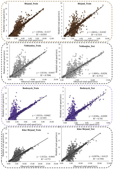
Figure A2.
Scattered plots of observed and modeled values of WS by meta-algorithm at different stations.
Figure A2.
Scattered plots of observed and modeled values of WS by meta-algorithm at different stations.
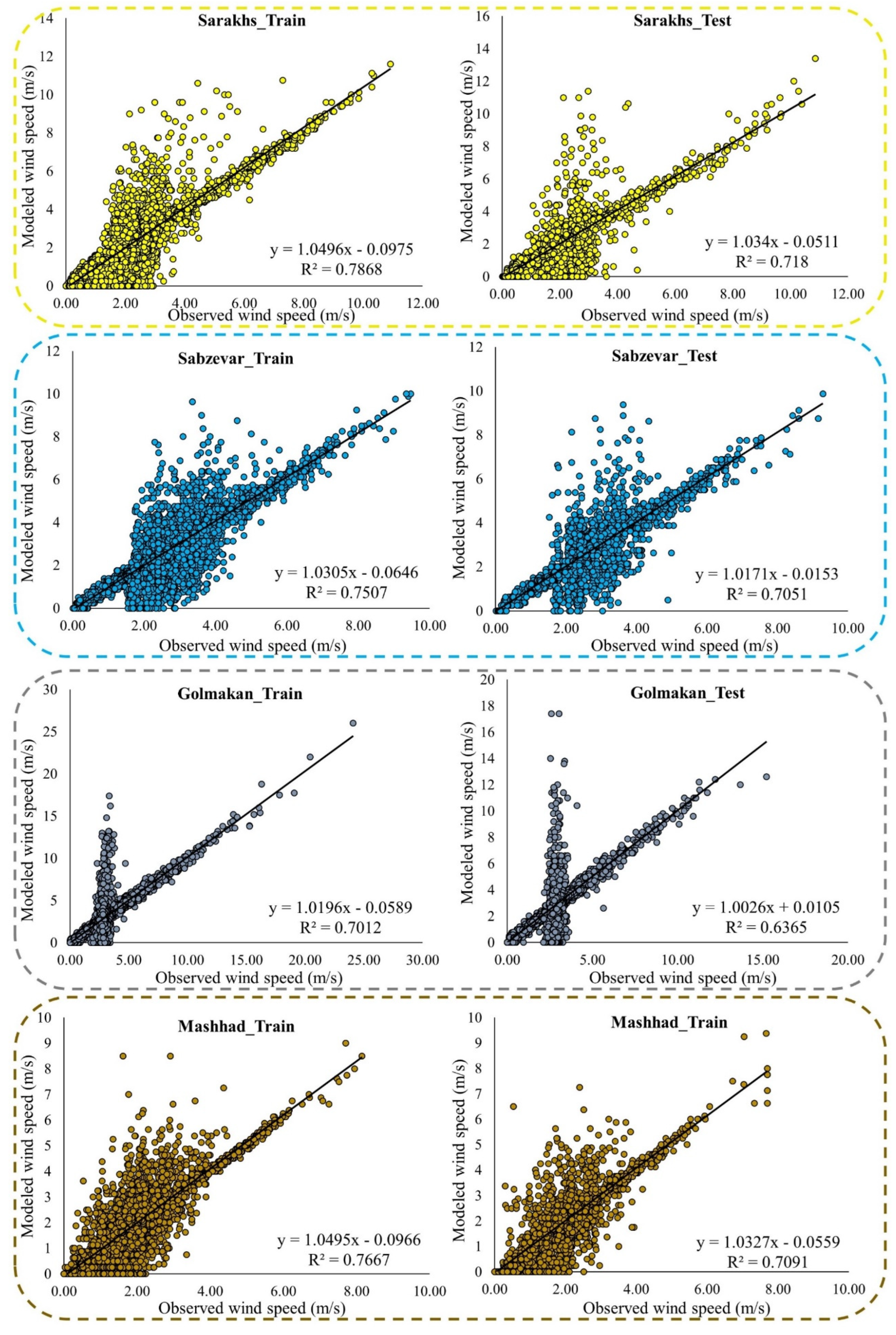
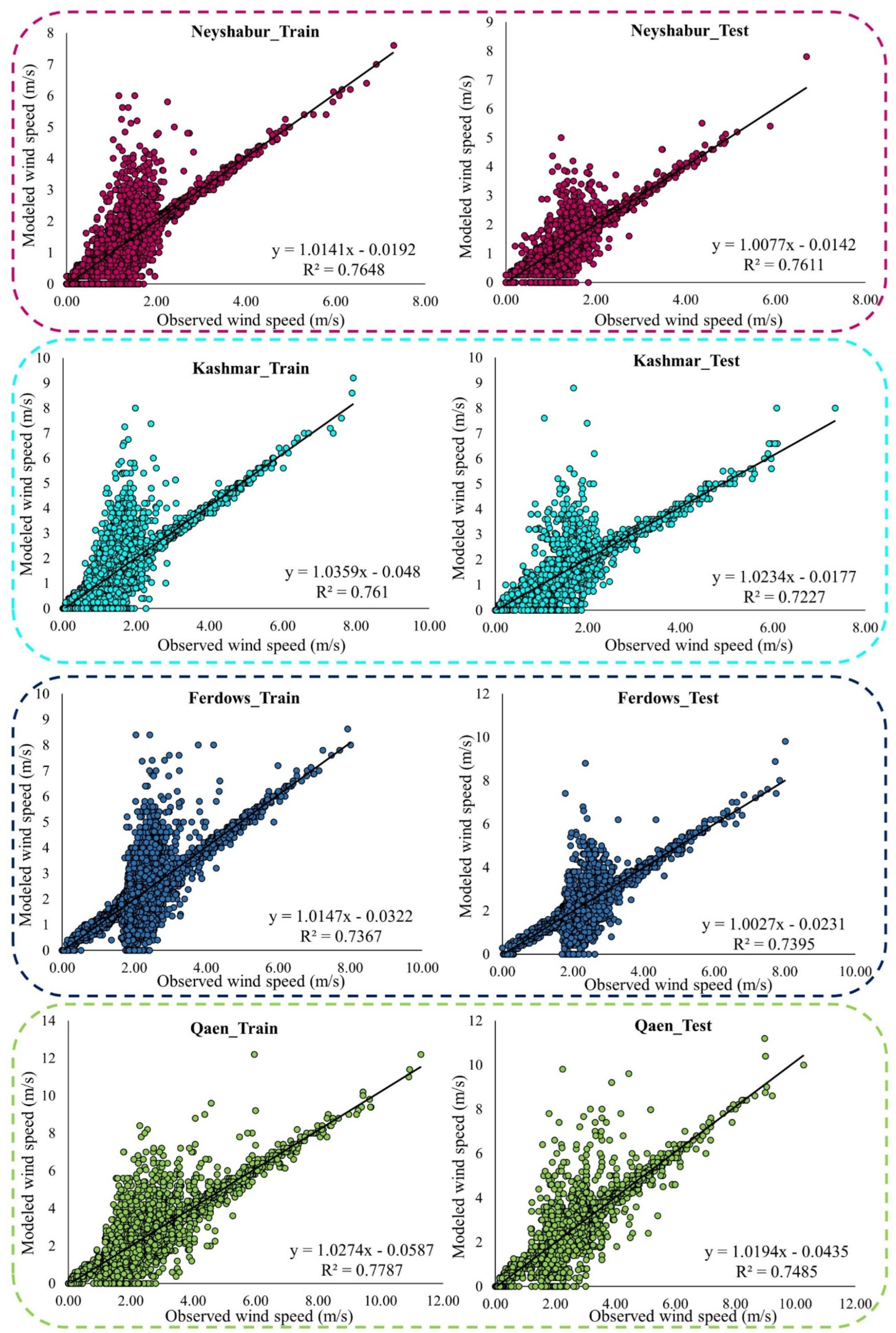
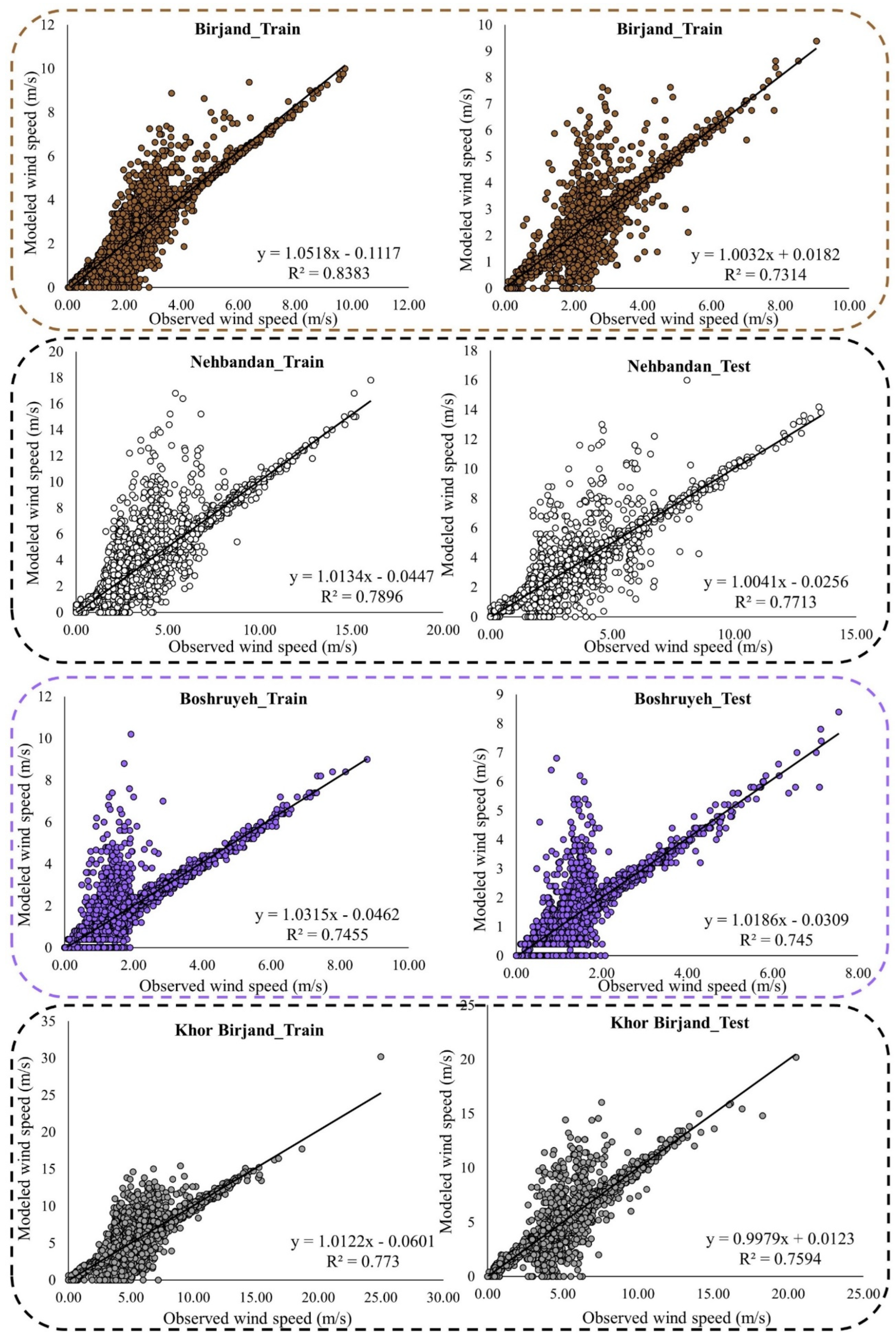
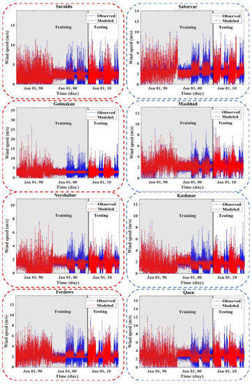
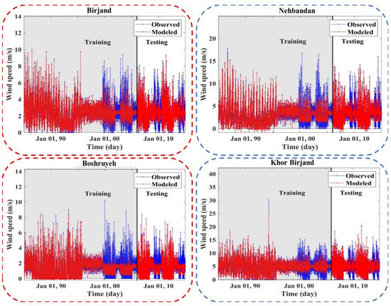
Figure A3.
Time series of observed and modeled values of WS using the meta-algorithm at different stations.
Figure A3.
Time series of observed and modeled values of WS using the meta-algorithm at different stations.

Appendix D
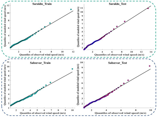
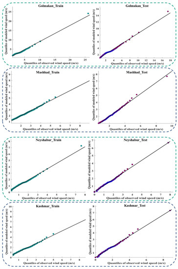
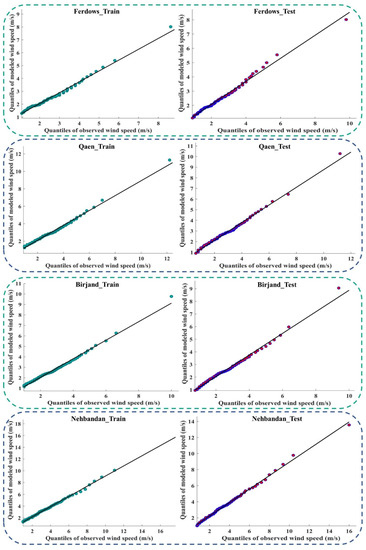

Figure A4.
Q–Q plots of the observed and modeled values of WS using the meta-algorithm at different stations.
Figure A4.
Q–Q plots of the observed and modeled values of WS using the meta-algorithm at different stations.
References
- Singh, U.; Rizwan, M.; Alaraj, M.; Alsaidan, I. A Machine Learning-Based Gradient Boosting Regression Approach for Wind Power Production Forecasting: A Step towards Smart Grid Environments. Energies 2021, 14, 5196. [Google Scholar] [CrossRef]
- Jung, C.; Schindler, D. Integration of small-scale surface properties in a new high resolution global wind speed model. Energy Convers. Manag. 2020, 210, 112733. [Google Scholar] [CrossRef]
- Busico, G.; Kazakis, N.; Cuoco, E.; Colombani, N.; Tedesco, D.; Voudouris, K.; Mastrocicco, M. A novel hybrid method of specific vulnerability to anthropogenic pollution using multivariate statistical and regression analyses. Water Res. 2020, 171, 115386. [Google Scholar] [CrossRef] [PubMed]
- Farzin, S.; Chianeh, F.N.; Anaraki, M.V.; Mahmoudian, F. Introducing a framework for modeling of drug electrochemical removal from wastewater based on data mining algorithms, scatter interpolation method, and multi criteria decision analysis (DID). J. Clean. Prod. 2020, 266, 122075. [Google Scholar] [CrossRef]
- Kadkhodazadeh, M.; Farzin, S. A Novel LSSVM Model Integrated with GBO Algorithm to Assessment of Water Quality Parameters. Water Resour. Manag. 2021, 35, 3939–3968. [Google Scholar] [CrossRef]
- Jha, M.K.; Shekhar, A.; Jenifer, M.A. Assessing groundwater quality for drinking water supply using hybrid fuzzy-GIS-based water quality index. Water Res. 2020, 179, 115867. [Google Scholar] [CrossRef]
- Ghorbani, M.A.; Jabehdar, M.A.; Yaseen, Z.M.; Inyurt, S. Solving the pan evaporation process complexity using the development of multiple mode of neurocomputing models. Theor. Appl. Climatol. 2021, 145, 1521–1539. [Google Scholar] [CrossRef]
- Zhou, J.; Shi, J.; Li, G. Fine tuning support vector machines for short-term wind speed forecasting. Energy Convers. Manag. 2011, 52, 1990–1998. [Google Scholar] [CrossRef]
- Panapakidis, I.P.; Dagoumas, A.S. Day-ahead electricity price forecasting via the application of artificial neural network based models. Appl. Energy 2016, 172, 132–151. [Google Scholar] [CrossRef]
- Fogno Fotso, H.R.; Aloyem Kazé, C.V.; Djuidje Kenmoé, G.A. A novel hybrid model based on weather variables relationships improving applied for wind speed forecasting. Int. J. Energy. Environ. Eng. 2022, 13, 43–56. [Google Scholar] [CrossRef]
- Elsisi, M.; Tran, M.Q.; Mahmoud, K.; Lehtonen, M.; Darwish, M.M.F. Robust design of ANFIS-based blade pitch controller for wind energy conversion systems against wind speed fluctuations. IEEE Access 2021, 9, 37894–37904. [Google Scholar] [CrossRef]
- Huang, X.; Wang, J.; Huang, B. Two novel hybrid linear and nonlinear models for wind speed forecasting. Energy Convers. Manag. 2021, 238, 114162. [Google Scholar] [CrossRef]
- Wang, J.; Li, H.; Wang, Y.; Lu, H. A hesitant fuzzy wind speed forecasting system with novel defuzzification method and multi-objective optimization algorithm. Expert Syst. Appl. 2021, 168, 114364. [Google Scholar] [CrossRef]
- Chen, X.J.; Zhao, J.; Jia, X.Z.; Li, Z.L. Multi-step wind speed forecast based on sample clustering and an optimized hybrid system. Renew Energy 2021, 165, 595–611. [Google Scholar] [CrossRef]
- Du, P.; Wang, J.; Yang, W.; Niu, T. A novel hybrid model for short-term wind power forecasting. Appl. Soft Comput. 2019, 80, 93–106. [Google Scholar] [CrossRef]
- Cheng, Z.; Wang, J. A new combined model based on multi-objective salp swarm optimization for wind speed forecasting. Appl. Soft Comput. 2020, 92, 106294. [Google Scholar] [CrossRef]
- Chen, Y.; Dong, Z.; Wang, Y.; Su, J.; Han, Z.; Zhou, D.; Zhang, K.; Zhao, Y.; Bao, Y. Short-term wind speed predicting framework based on EEMD-GA-LSTM method under large scaled wind history. Energy Convers. Manag. 2021, 227, 113559. [Google Scholar] [CrossRef]
- Liu, H.; Duan, Z.; Chen, C.; Wu, H. A novel two-stage deep learning wind speed forecasting method with adaptive multiple error corrections and bivariate Dirichlet process mixture model. Energy Convers. Manag. 2019, 199, 111975. [Google Scholar] [CrossRef]
- Liu, Y.; Qin, H.; Zhang, Z.; Pei, S.; Jiang, Z.; Feng, Z.; Zhou, J. Probabilistic spatiotemporal wind speed forecasting based on a variational Bayesian deep learning model. Appl. Energy 2020, 260, 114259. [Google Scholar] [CrossRef]
- Neshat, M.; Nezhad, M.M.; Abbasnejad, E.; Mirjalili, S.; Tjernberg, L.B.; Astiaso Garcia, D.; Alexander, B.; Wagner, M. A deep learning-based evolutionary model for short-term wind speed forecasting: A case study of the Lillgrund offshore wind farm. Energy Convers. Manag. 2021, 236, 114002. [Google Scholar] [CrossRef]
- Liu, X.; Lin, Z.; Feng, Z. Short-term offshore wind speed forecast by seasonal ARIMA—A comparison against GRU and LSTM. Energy 2021, 227, 120492. [Google Scholar] [CrossRef]
- Wang, J.; Li, Y. Multi-step ahead wind speed prediction based on optimal feature extraction, long short term memory neural network and error correction strategy. Appl. Energy 2018, 230, 429–443. [Google Scholar] [CrossRef]
- Liang, T.; Zhao, Q.; Lv, Q.; Sun, H. A novel wind speed prediction strategy based on Bi-LSTM, MOOFADA and transfer learning for centralized control centers. Energy 2021, 230, 120904. [Google Scholar] [CrossRef]
- Xie, A.; Yang, H.; Chen, J.; Sheng, L.; Zhang, Q.; Kumar Jha, S.; Zhang, X.; Zhang, L.; Patel, N. A Short-Term Wind Speed Forecasting Model Based on a Multi-Variable Long Short-Term Memory Network. Atmosphere 2021, 12, 651. [Google Scholar] [CrossRef]
- Fu, W.; Zhang, K.; Wang, K.; Wen, B.; Fang, P.; Zou, F. A hybrid approach for multi-step wind speed forecasting based on two-layer decomposition, improved hybrid DE-HHO optimization and KELM. Renew Energy 2021, 164, 211–229. [Google Scholar] [CrossRef]
- Ibrahim, A.; Mirjalili, S.; El-Said, M.; Ghoneim, S.S.M.; Al-Harthi, M.M.; Ibrahim, T.F.; El-Kenawy, E.S.M. Wind Speed Ensemble Forecasting Based on Deep Learning Using Adaptive Dynamic Optimization Algorithm. IEEE Access 2021, 9, 125787–125804. [Google Scholar] [CrossRef]
- Qu, Z.; Zhang, K.; Mao, W.; Wang, J.; Liu, C.; Zhang, W. Research and application of ensemble forecasting based on a novel multi-objective optimization algorithm for wind-speed forecasting. Energy Convers. Manag. 2017, 154, 440–454. [Google Scholar] [CrossRef]
- Liu, Z.; Jiang, P.; Wang, J.; Zhang, L. Ensemble forecasting system for short-term wind speed forecasting based on optimal sub-model selection and multi-objective version of mayfly optimization algorithm. Expert Syst. Appl. 2021, 177, 114974. [Google Scholar] [CrossRef]
- Karthikeyan, M.; Rengaraj, R. Short-term wind speed forecasting using ensemble learning. In Proceedings of the 7th International Conference on Electrical Energy Systems (ICEES), Chennai, India, 11–13 February 2021; pp. 502–506. [Google Scholar] [CrossRef]
- Sloughter, J.M.L.; Gneiting, T.; Raftery, A.E. Probabilistic Wind Speed Forecasting Using Ensembles and Bayesian Model Averaging. J. Am. Stat. Assoc. 2012, 105, 25–35. [Google Scholar] [CrossRef] [Green Version]
- Valikhan Anaraki, M.; Mahmoudian, F.; Nabizadeh Chianeh, F.; Farzin, S. Dye Pollutant Removal from Synthetic Wastewater: A New Modeling and Predicting Approach Based on Experimental Data Analysis, Kriging Interpolation Method, and Computational Intelligence Techniques. J. Environ. Inform. 2022. [CrossRef]
- Tikhamarine, Y.; Malik, A.; Souag-Gamane, D.; Kisi, O. Artificial intelligence models versus empirical equations for modeling monthly reference evapotranspiration. Environ. Sci. Pollut. Res. 2020, 27, 30001–30019. [Google Scholar] [CrossRef] [PubMed]
- Lesar, T.T.; Filipčić, A. The Hourly Simulation of PM2.5 Particle Concentrations Using the Multiple Linear Regression (MLR) Model for Sea Breeze in Split, Croatia. Water Air Soil Pollut. 2021, 232, 261. [Google Scholar] [CrossRef]
- Kadkhodazadeh, M.; Anaraki, M.V.; Morshed-Bozorgdel, A.; Farzin, S. A New Methodology for Reference Evapotranspiration Prediction and Uncertainty Analysis under Climate Change Conditions Based on Machine Learning, Multi Criteria Decision Making and Monte Carlo Methods. Sustainability 2022, 14, 2601. [Google Scholar] [CrossRef]
- Huangfu, W.; Wu, W.; Zhou, X.; Lin, Z.; Zhang, G.; Chen, R.; Song, Y.; Lang, T.; Qin, Y.; Ou, P.; et al. Landslide Geo-Hazard Risk Mapping Using Logistic Regression Modeling in Guixi, Jiangxi, China. Sustainability 2021, 13, 4830. [Google Scholar] [CrossRef]
- Salehi, M.; Farhadi, S.; Moieni, A.; Safaie, N.; Hesami, M. A hybrid model based on general regression neural network and fruit fly optimization algorithm for forecasting and optimizing paclitaxel biosynthesis in Corylus avellana cell culture. Plant Methods 2021, 17, 13. [Google Scholar] [CrossRef] [PubMed]
- Sridharan, M. Generalized Regression Neural Network Model Based Estimation of Global Solar Energy Using Meteorological Parameters. Ann. Data Sci. 2021. [CrossRef]
- Friedman, J.H. Multivariate Adaptive Regression Splines. Ann. Stat. 1991, 19, 1–67. [Google Scholar] [CrossRef]
- Quinlan, J.R.; Quinlan, J.R. Learning with Continuous Classes. In Proceedings of the 5th Australian Joint Conference on Artificial Intelligence, Hobart, Austrilia, 16–18 November 1992; World Scientific: Singapore, 1992; pp. 343–348. [Google Scholar] [CrossRef]
- Emamifar, S.; Rahimikhoob, A.; Noroozi, A.A. An Evaluation of M5 Model Tree vs. Artificial Neural Network for Estimating Mean Air Temperature as Based on Land Surface Temperature Data by MODIS-Terra Sensor. Iran. J. Soil Water Res. 2014, 45, 423–433. [Google Scholar] [CrossRef]
- Bharti, B.; Pandey, A.; Tripathi, S.K.; Kumar, D. Modelling of runoff and sediment yield using ANN, LS-SVR, REPTree and M5 models. Hydrol. Res. 2017, 48, 1489–1507. [Google Scholar] [CrossRef]
- Arumugam, P.; Chemura, A.; Schauberger, B.; Gornott, C. Remote Sensing Based Yield Estimation of Rice (Oryza Sativa L.) Using Gradient Boosted Regression in India. Remote Sens. 2021, 13, 2379. [Google Scholar] [CrossRef]
- Wen, H.T.; Lu, J.H.; Phuc, M.X. Applying Artificial Intelligence to Predict the Composition of Syngas Using Rice Husks: A Comparison of Artificial Neural Networks and Gradient Boosting Regression. Energies 2021, 14, 2932. [Google Scholar] [CrossRef]
- Pazouki, G.; Golafshani, E.M.; Behnood, A. Predicting the compressive strength of self-compacting concrete containing Class F fly ash using metaheuristic radial basis function neural network. Struct. Concr. 2021, 23, 1191–1213. [Google Scholar] [CrossRef]
- Ojo, S.; Imoize, A.; Alienyi, D. Radial basis function neural network path loss prediction model for LTE networks in multitransmitter signal propagation environments. Int. J. Commun. Syst. 2021, 34, e4680. [Google Scholar] [CrossRef]
- Friedman, J.H. Greedy function approximation: A gradient boosting machine. Ann. Statist. 2001, 29, 1189–1232. [Google Scholar] [CrossRef]
- Suykens, J.A.K.; Van Gestel, T.; De Brabanter, J.; De Moor, B.; Vandewalle, J. Least Squares Support Vector Machines; World Scientific: Singapore, 2002. [Google Scholar] [CrossRef]
- Farzin, S.; Valikhan Anaraki, M. Modeling and predicting suspended sediment load under climate change conditions: A new hybridization strategy. J. Water Clim. Chang. 2021, 12, 2422–2443. [Google Scholar] [CrossRef]
- Heidari, A.A.; Mirjalili, S.; Faris, H.; Aljarah, I.; Mafarja, M.; Chen, H. Harris hawks optimization: Algorithm and applications. Future Gener. Comput. Syst. 2019, 97, 849–872. [Google Scholar] [CrossRef]
- Houssein, E.H.; Hosney, M.E.; Oliva, D.; Mohamed, W.M.; Hassaballah, M. A novel hybrid Harris hawks optimization and support vector machines for drug design and discovery. Comput. Chem. Eng. 2020, 133, 106656. [Google Scholar] [CrossRef]
- Bhuiyan, E.; Cerrai, D.; Biswas, N.K.; Zhang, H.; Wang, Y.; Chen, D.; Feng, D.; You, X.; Wu, W. Temperature Forecasting Correction Based on Operational GRAPES-3km Model Using Machine Learning Methods. Atmosphere 2022, 13, 362. [Google Scholar] [CrossRef]
- Valikhan Anaraki, M.; Farzin, S.; Mousavi, S.F.; Karami, H. Uncertainty Analysis of Climate Change Impacts on Flood Frequency by Using Hybrid Machine Learning Methods. Water Resour. Manag. 2021, 31, 199–223, 101007/s11269. [Google Scholar] [CrossRef]
Publisher’s Note: MDPI stays neutral with regard to jurisdictional claims in published maps and institutional affiliations. |
© 2022 by the authors. Licensee MDPI, Basel, Switzerland. This article is an open access article distributed under the terms and conditions of the Creative Commons Attribution (CC BY) license (https://creativecommons.org/licenses/by/4.0/).

