Air Quality and Behavioral Impacts of Anti-Idling Campaigns in School Drop-Off Zones

Abstract

Vehicle emissions are a major source of pollution in urban communities and idling may contribute up to 34% or more to local air pollution levels. Reduced idling has been found to be an effective policy tool for improving air quality, especially around schools, where it may also improve outcomes for asthmatic children. We studied two anti-idling campaigns in Salt Lake County, Utah to understand if reduced engine idling leads to behavioral change and subsequent reduction in traffic-related air pollution exposure of the related school. We found a 38% decrease in idling time following an anti-idling campaign and an 11% decrease in the number of vehicles idling at the school drop-off zones. The air quality measurements showed improvement in the middle of the campaign, but seasonal variability as well as atmospheric inversion events had substantial effects on overall ambient pollutant concentrations. This study provides an encouraging starting point to develop more effective anti-idling campaigns to protect the health of children, school staff, and the surrounding community.

1. Introduction

Idling is the simple act of running an engine while the vehicle is not in motion or in gear. Although the behavior seems harmless, idling is a substantial contributor to air pollution [1] and associated health impacts. Vehicle emissions are a major source of pollution in rural and urban communities and idling may contribute up to 34% or more to local air pollution levels [2]. In addition, countless studies suggest that there is no benefit to this behavior (i.e., economic or technical) [3] and that the behavior is more likely to waste money and natural resources. For example, vehicle emissions from idling can damage vehicles, pollute the air, reduce economic and educational outcomes, impact human health, and lead to increased mortality [4,5,6]. Although the time we spend in vehicles is short, the potential exposure to high levels of pollutants should not be overlooked. For instance, Barnes et al. [7] note that pollutants were higher inside the vehicle with an idle engine in contrast to the vehicle during driving. Additionally, since the transportation sector contributes substantially to fossil fuel consumption, greenhouse gas (GHG) emissions, and poor air quality, it also contributes to respiratory health hazards [8]. These findings illustrate how anti-idling policies are a good strategy to manage air pollution.

Anti-idling policies also appear to have their greatest potential in the school setting. When traffic-related emissions are the dominant pollution source in the school vicinity, the changes in outdoor air quality associated with the anti-idling campaign are capable of reducing the children’s exposure to traffic-generated aerosols inside the schools at a statistically significant level [9]. Lee et al. [10] were among the first to show idling has massive impacts on ambient air quality in and around a school. In their early work on this topic, they found idling resulted in significant increases in atmospheric fine particulate matter (PM_2.5), ultrafine particulate matter (PM_0.1), polycyclic aromatic hydrocarbons (PAHs), and black carbon (BC) levels by 16.5%, 33.3%, 48.0%, and 11.5%, respectively. Consequently, the restriction of local idling emission was proven to significantly reduce particulate matter and harmful pollutants in the hot spots around the school environment. These findings were later explained by Macneill et al. [11], who showed that since many schools are situated closer to major roads and children spend much of their day in school, efforts should be made to reduce traffic-related air pollutant concentrations in the school environments.

The good news is that large-scale testing of idling interventions repeatedly shows that simply reminding individuals to shut off their engine during long waits in the vehicle significantly improved the behavior and dramatically reduced pollution concentrations in and around the area [12]. In multiple places across the globe, the impacts of grassroot campaigns to clean the air through information and subsequent action campaigns have gained significant traction. For example, in Krakow, Poland, a smog alert action campaign combined with legislation on solid fuel heating drastically cut air pollution in the last decade [13] and estimated potential impacts of policy-driven reductions [14]. Likewise, reducing idling has been found to be an effective policy tool for improving outcome for asthmatic children in schools [15]. Kim et al. [9] show a similar pattern in their work, but found concentrations were highest in schools near roadways, which further prevented rapid dispersion of pollutants. Finally, Kinsey, Williams, Dong and Logan [3] show that even with factors such as engine pulse and restart, shutting down engines in school buses and restarting the bus just before departure is the preferred operating scenario as long as there is no extended idling after the engine is restarted. Based on these prior studies, it is clear that idling prevention may have high value as a policy instrument, especially in schools.

To assess the effectiveness of this public health initiative (e.g., idling intervention), we compare and contrast the findings from two anti-idling campaigns in Salt Lake County, Utah. The goal of this study is to understand if reduced engine idling leads to the subsequent reduction in traffic-related air pollution exposure of the related school communities.

2. Materials and Methods

2.1. Anti-Idling Campaigns

Anti-idling campaigns were carried out at two elementary schools, both located in Salt Lake County, Utah (Figure 1 and Figure 2). One campaign took place at Willow Springs Elementary in January 2020 while the other was a two-phase campaign at Bonneville Elementary: Phase 1 during September 2019 and Phase 2 during February 2020. The state of Utah is one of the fastest-growing states in the United States and has substantial air quality concerns in its urban centers, especially in the lower-elevation areas. According to a 2021 report by the American Lung Association, Salt Lake City (SLC) is the 12th most polluted city nationwide for ozone pollution and the 17th most polluted city in the US for short-term particulate pollution [16]. There are multiple contributing factors to this phenomenon.

As illustrated in Figure 1, SLC is located at the intersection of two major highways (e.g., I-80 and I-15) and therefore transportation-related emissions are an important contributor to poor air quality. Like many urban areas, traffic density and congestion in Salt Lake County (SLCo) have been increasing by approximately 10% or more annually [17], making this and other urban areas increasingly susceptible to transportation-related air pollution. Emissions from the traffic sector (primarily NO_x and volatile organic compounds—VOC) have decreased over the last decade due to improved fuels (Tier 3), improved fuel efficiency, and increased emission controls. However, increased traffic density is offsetting, to some extent, the gains seen as a result of these emission reductions. Additionally, SLCo has unique geography with multiple intersecting high mountain ranges and the Great Salt Lake, surrounding expansive residential housing and a range of industries (Figure 1). Air pollution problems in SLCo are further exacerbated by both transported and local production of pollution associated with regional dust storms. As a result, both the summer and winter months are impacted by elevated ozone [18] and PM_2.5 [19], respectively, affecting indoor air quality as well [20].

2.2. Instrument Description

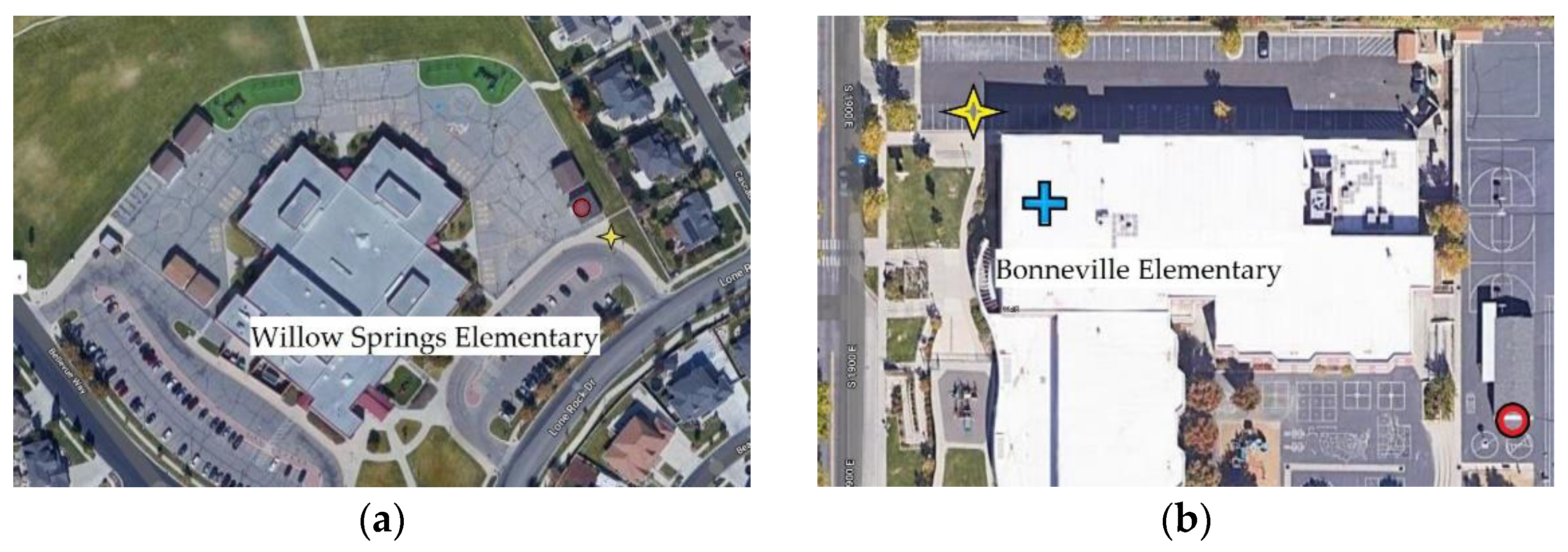
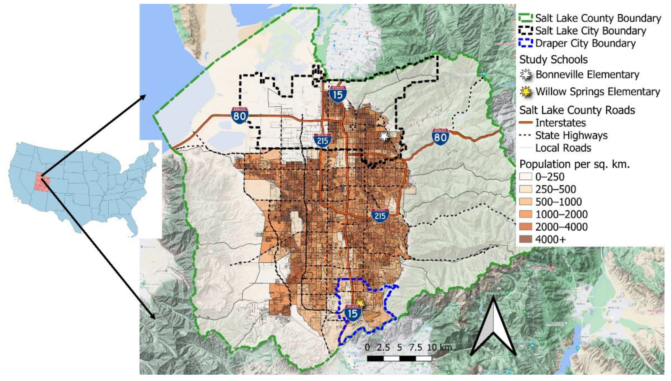
This study deployed research-grade sensors, which are demonstrated to be comparable to regulatory-grade instrumentation in accuracy and precision [21] and significantly more robust and reliable than commonly used low-cost or citizen science sensors [22]. In addition, a mobile laboratory was used as a pseudo-stationary near surface measurement platform and parked near or at drop-off locations at the two schools. Instrumentation and the vehicle platform are described in detail in Bush et al. [23], Hopkins et al. [24]. In short, the mobile lab housed a suite of research-grade instrumentation making high frequency greenhouse gas and air quality observations. Carbon dioxide (CO₂), methane (CH₄) and atmospheric water vapor (H₂O) were measured using a Los Gatos Research Ultra-portable Greenhouse Gas Analyzer. Atmospheric ozone was measured using a 2B Technologies Model 205 monitor with a tolerance of 2% [25]. Nitrogen oxides concentrations were measured using a 2B Technologies Model 410 monitor. PM_2.5 was measured using a MetOne Instruments ES-642 Remote Dust Monitor with a tolerance of 1 µg m⁻³ [26]. Meteorological parameters including wind speed and direction, temperature and relative humidity were all measured using an AirMar 200 WX weather station.

Regular calibration of the instruments used in this study were conducted according to standard recommended protocols. Previous studies have previously validated the research-grade PM_2.5 sensors used in this study against regulatory grade (FEM, or Federal Equivalent Method) monitors [21,27]. The 2B ozone sensors used in this study are FEM, or Federal Equivalent Method, but were also compared against Utah Division of Air Quality Sensors and shown to be highly accurate when validated against state air pollution monitoring sites [21,27].

2.3. Study Site

The schools in the focus of this study are found on opposite sides of SLCo (Figure 1). Willow Springs Elementary (“Willow Springs”) (40.50965° N, 111.87747° W [28], Elevation 1359 MASL [29]) and Bonneville Elementary (“Bonneville”) (40.74424° N, 111.83613° W, Elevation 1420 MASL) are located approximately 26.5 km apart, nearly directly aligned North–South.

At each school (Figure 2), the van was parked in the main parking lot near the drop-off zone. Using the same instruments described in Section 2.2, PM_2.5 and ozone instruments were installed the playground and an additional ozone sensor was located indoors at the K6 multipurpose area at Bonneville (Figure 2b).

The main anthropogenic emission sources for the pollutants in this study in Utah, and particularly the highly urbanized Salt Lake County, are on-road vehicles, followed by area sources [30,31]. Highly trafficked interstates I-15 and I-80 are close to both schools, and while there are no major point sources near the study sites, they are both surrounded by residential areas. Between November and February each year, SLC experiences periodic episodes of persistent temperature inversions, where pollutants accumulate and forms through secondary reactions in the stable boundary layer for several days to several weeks [19,32,33]. By April and May, solar insolation is strong enough that generally only nocturnal inversions are noted, and pollution does not build up in the valleys to the extent it does earlier in the year. However, elevated ozone concentrations are found between May and September [18]. The study period in this study (September 2019–February 2020) is thus representative of both the late summer/early fall through middle of the winter inversion season. The air pollution measurement campaign duration along with the study sensors are listed in

Table 1. Campaign timelines including sensor availability.

Site	Pollutant	Willow Springs	Bonneville Phase 1	Bonneville Phase 2
Van	CH4, CO2, NOx, PM2.5, O3	10–17 January 2020	16–20 September 2019	14–21 February 2020
Playground	PM2.5	-	13–27 September 2019	13–26 February 2020
	O3	-	13–27 September 2019	14–26 February 2020
School (Indoor)	PM2.5	15–28 January 2020	-	-
	O3	-	16–27 September 2019	21–26 February 2020

. Spearman correlation tests were used to compare van pollutant measurement results and, where available, measurements across sites (van, playground, and school).

2.4. Vehicle Count Campaign

Vehicle counts as well as idling duration for each vehicle were conducted for Tuesday to Friday for each of the two Bonneville study phases as part of the “Idle-Free Campaign”. Bonneville Phase 1 was considered the pre-campaign period and Bonneville Phase 2 was considered the post-campaign period. Measurements were taken at five locations surrounding Bonneville Elementary during the morning drop-off (8:00–8:45 a.m.), midday (12:35–1:05 p.m.), and afternoon pick-up (2:45–3:15 p.m.) periods. The campaign and observations were based on the EPA’s Idle-Free Campaign and modified by the focus group and survey conducted the year before as well as input by the Bonneville Elementary PTA and Bonneville Elementary Clean Air Committee. Observations were conducted by parent volunteers, Bonneville Elementary Clean Air Committee members, and study authors. Parents noted when vehicles arrived; if they were idling; if they were idling, for how long (in seconds); and when the vehicle left. The methodology was the same for the pre- and post-campaigns. All volunteers were instructed on methods by study authors.

3. Results

The results are divided into three subsections, one for each campaign/stage. Within each campaign substage, the first part discusses the pollutant time series, the second shows the Spearman correlation results of van pollutant measurements, and for the Bonneville campaigns, the third section also shows the Spearman correlation results of site pollutant measurements.

Table 2. Hourly mean and range (minimum–maximum) pollutant readings for each campaign.

Site	Pollutant	Willow Springs	Bonneville Phase 1	Bonneville Phase 2
Van	CH4 (ppm)	1.95 (1.90–2.26)	1.91 (1.86–2.07)	2.01 (1.92–2.38)
	CO2 (ppm)	430.29 (411.97–558.54)	414.78 (402.51–463.62)	439.33 (417.88–525.75)
	NOx (ppb)	7.81 (0.00–68.11)	4.54 (0.00–23.00)	5.46 (0.00–32.53)
	PM2.5 (µg/m3)	1.43 (0.02–6.62)	2.08 (0.42–5.56)	3.21 (0.30–10.50)
	O3 (ppb)	32.32 (27.89–54.36)	70.60 (36.93–82.95)	61.71 (32.78–79.00)
Playground	PM2.5 (µg/m3)	-	1.75 (0.20–7.68)	1.46 (0.02–7.23)
	O3 (ppb)	-	38.11 (2.32–69.16)	28.15 (0.00–52.2)
School (Indoor)	PM2.5 (µg/m3)	2.72 (0.08–12.60)	-	-
	O3 (ppb)	-	11.34 (2.28–31.03)	15.32 (0.00–36.03)

shows the hourly means as well as the minimum and maximum pollutant readings for each campaign. The seasonality effects are most clearly shown by the CO₂ measurements. Bonneville Phase 1 took place in September while Willow Springs and Bonneville Phase 2 took place in January and February, respectively. September is at the end of the growing season while January and February are not in the growing season and show substantially higher CO₂ values. Ozone has the opposite seasonal pattern, with higher outdoor values in the summer compared to winter. However, the van ozone measurements for the Bonneville campaigns were found to have a positive bias of approximately 30 ppb and caution should be used in their interpretation. Additionally, care must be taken in the interpretation of these results as the sensors measured different time lengths for each campaign as shown in Table 1.

3.1. Willow Springs

The Willow Springs campaign involved only the van parked at the main parking lot near the school drop-off zone. The first day (Friday, 10 January 2020) involved parking the van after school, at approximately 4 p.m. and it remained in place for seven days until it was picked up on Friday 17 January 2020 at approximately 3 p.m.

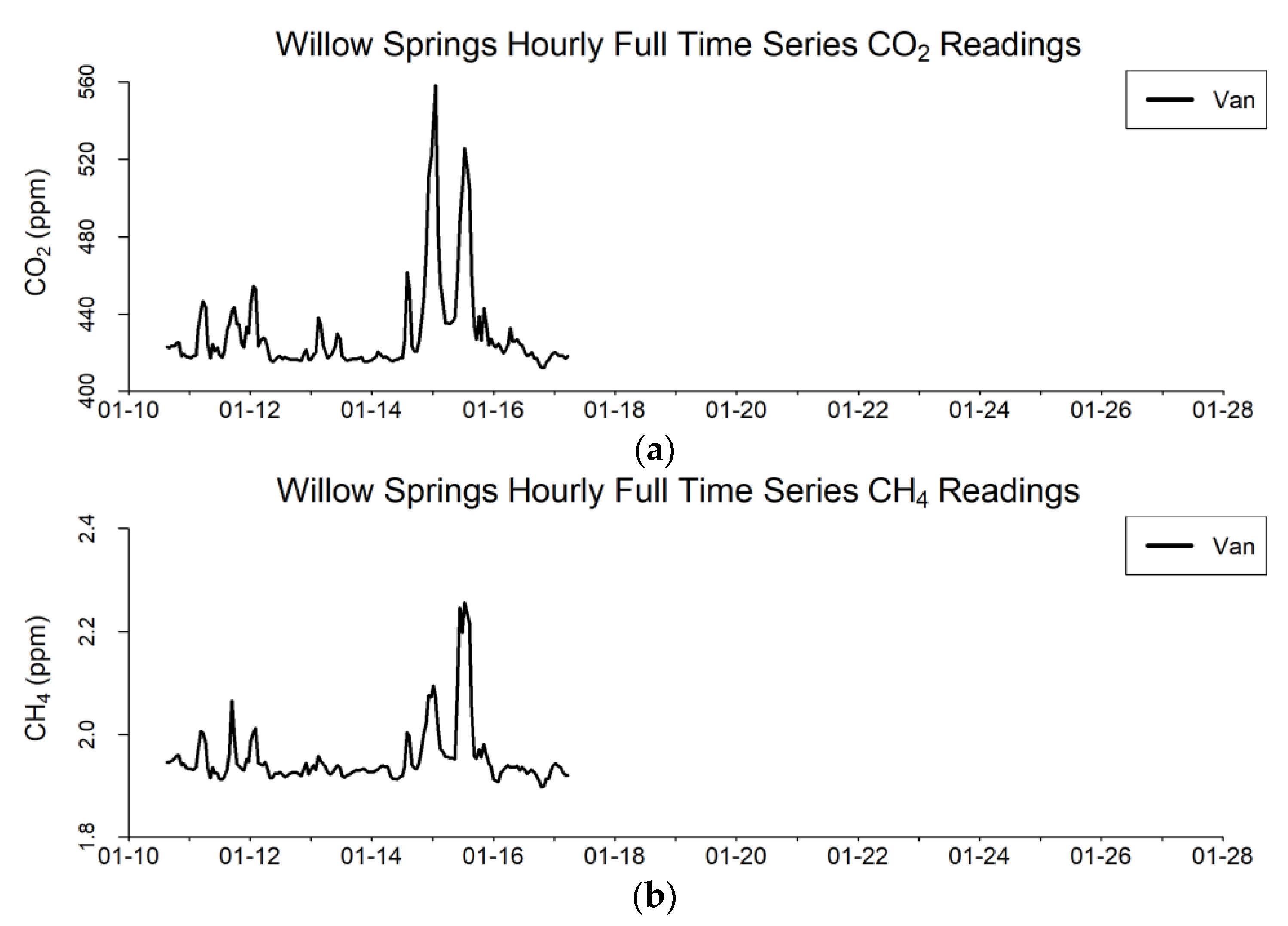
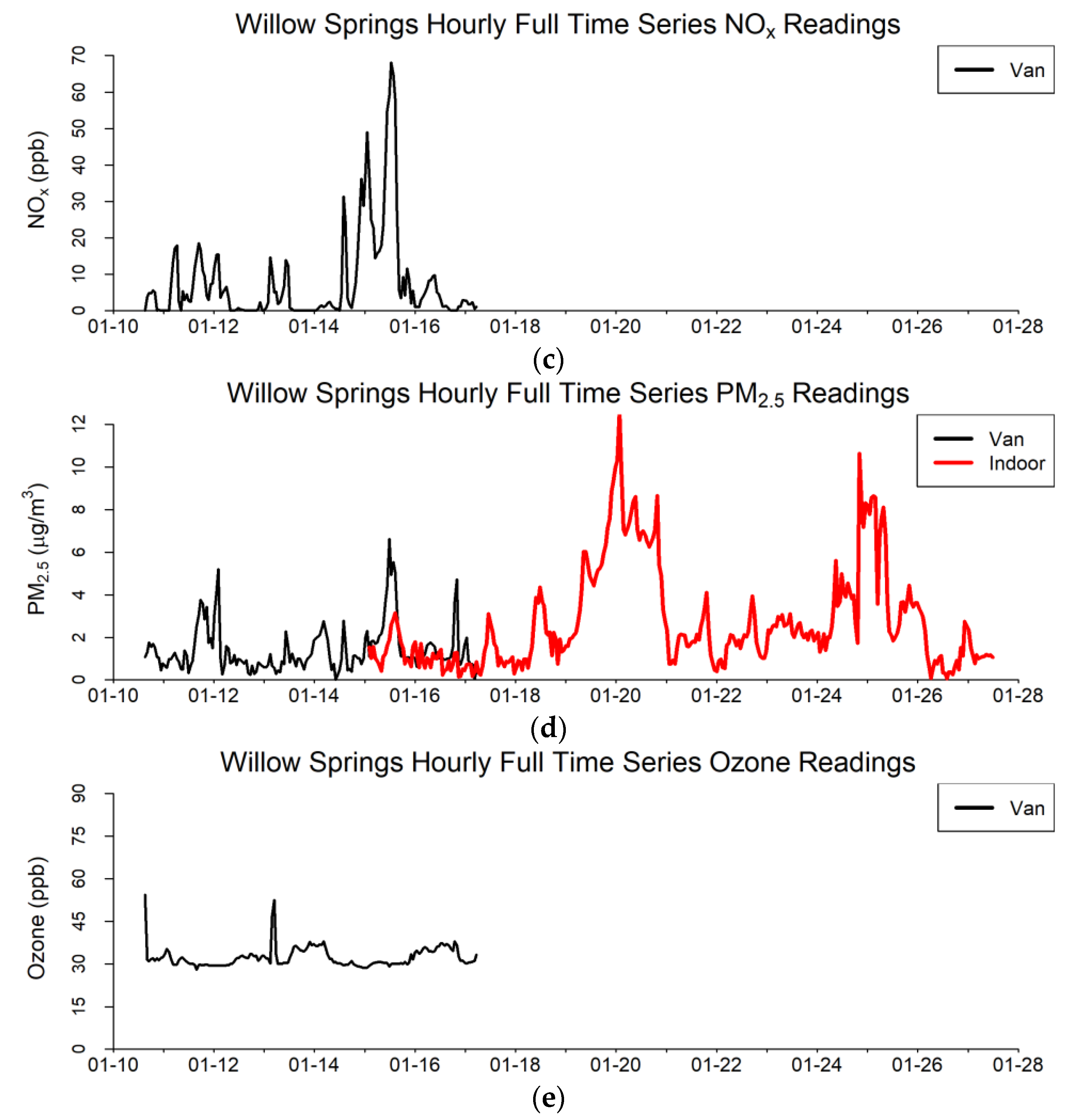
3.1.1. Van Outdoor Pollutant Time Series

The complete time series for the Willow Springs campaign for the five study pollutants is shown in Figure 3. The CO₂, CH₄, NO_x, and PM_2.5 (Figure 3a–d) series share similar features highlighting traffic rush hour patterns. This is most clearly noticeable during the atmospheric inversion event that took place on 14–17 January. During this event, pollutant concentrations rose particularly from 15 to 17 January due to the stagnation event. Of substantial interest is the comparison between NO_x and PM_2.5 patterns (Figure 3c,d). During persistent inversion events, secondary formation of PM_2.5 takes place using primary emissions of pollutants including NO_x. Therefore, while NO_x levels elevate earlier in the event (early part of 15 January), PM_2.5 lags NO_x and has an additional spike in the morning of 17 January. This peak is likely due to the lower boundary layer concentrating secondary PM_2.5 and is not reflected in the NO_x measurements. Ozone (Figure 3e) remains relatively consistent except for a peak early on 13 January.

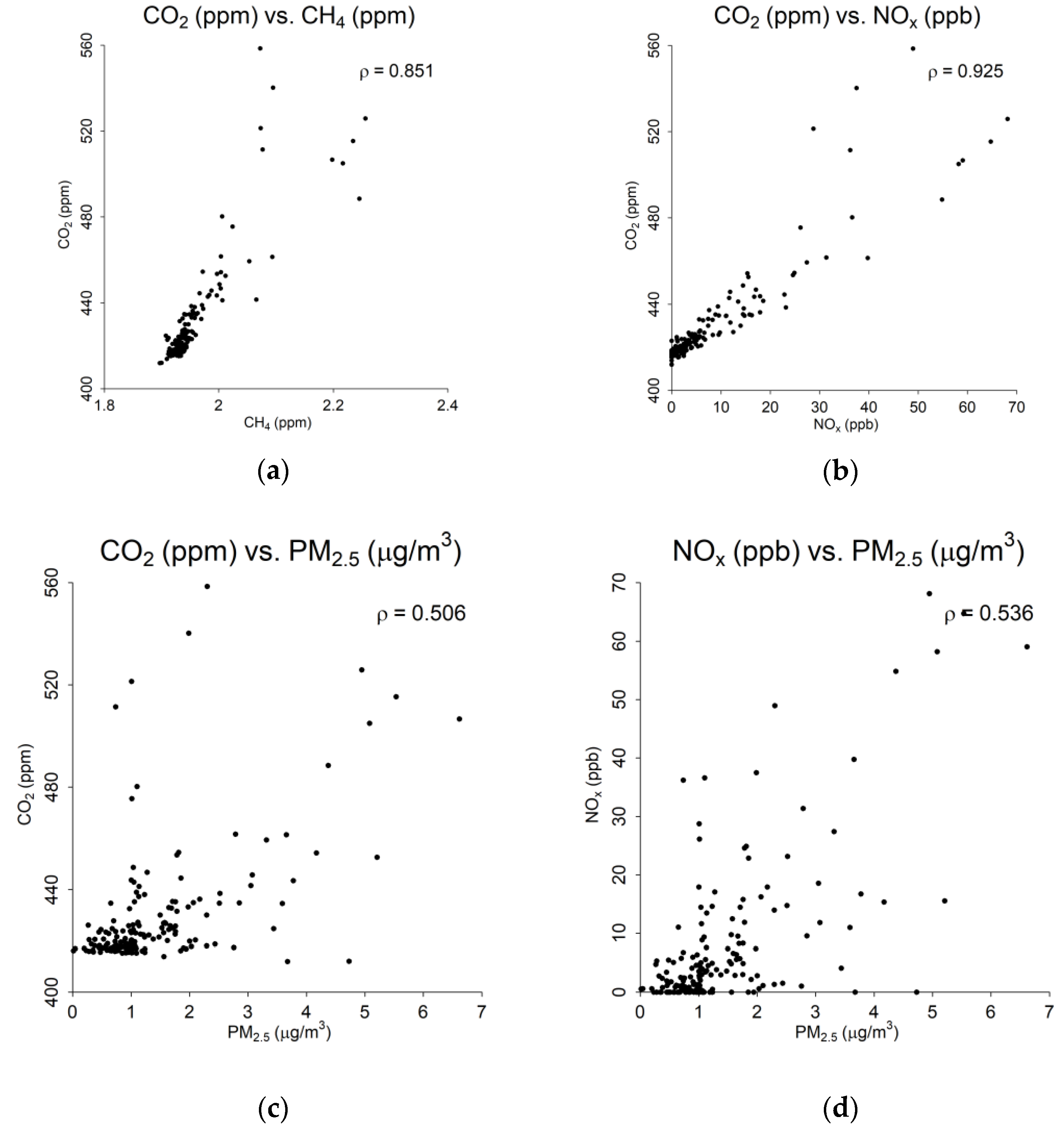
3.1.2. Van Outdoor Pollutant Comparison

The van pollutant comparisons are shown in

Table 3. Willow Springs campaign Spearman correlation test results for van pollutant readings.

Equipment	ρ (rho)	95% CI	p-Value
CO2 vs. CH4	0.851	0.793–0.909	<2.2 × 10−16
CO2 vs. NOx	0.925	0.894–0.957	<2.2 × 10−16
CO2 vs. PM2.5	0.505	0.374–0.637	<2.2 × 10−16
NOx vs. PM2.5	0.536	0.412–0.660	7.094 × 10−14

and Figure 4. The associations between pollutants show a close relationship between CO₂ and CH₄ (Figure 4a) as well as between CO₂ and NO_x (Figure 4b). This is to be expected as greenhouse gases generally track closely, and a substantial amount of CO₂ emissions are associated with traffic activity, which is the main contributor of NO_x. Due to the delayed formation of secondary PM_2.5 during the inversion event, described in Section 3.1.1, PM_2.5 shows a lower correlation to CO₂ and NO_x (Figure 4c,d). All the results were found to have a p-value of less than 0.001.

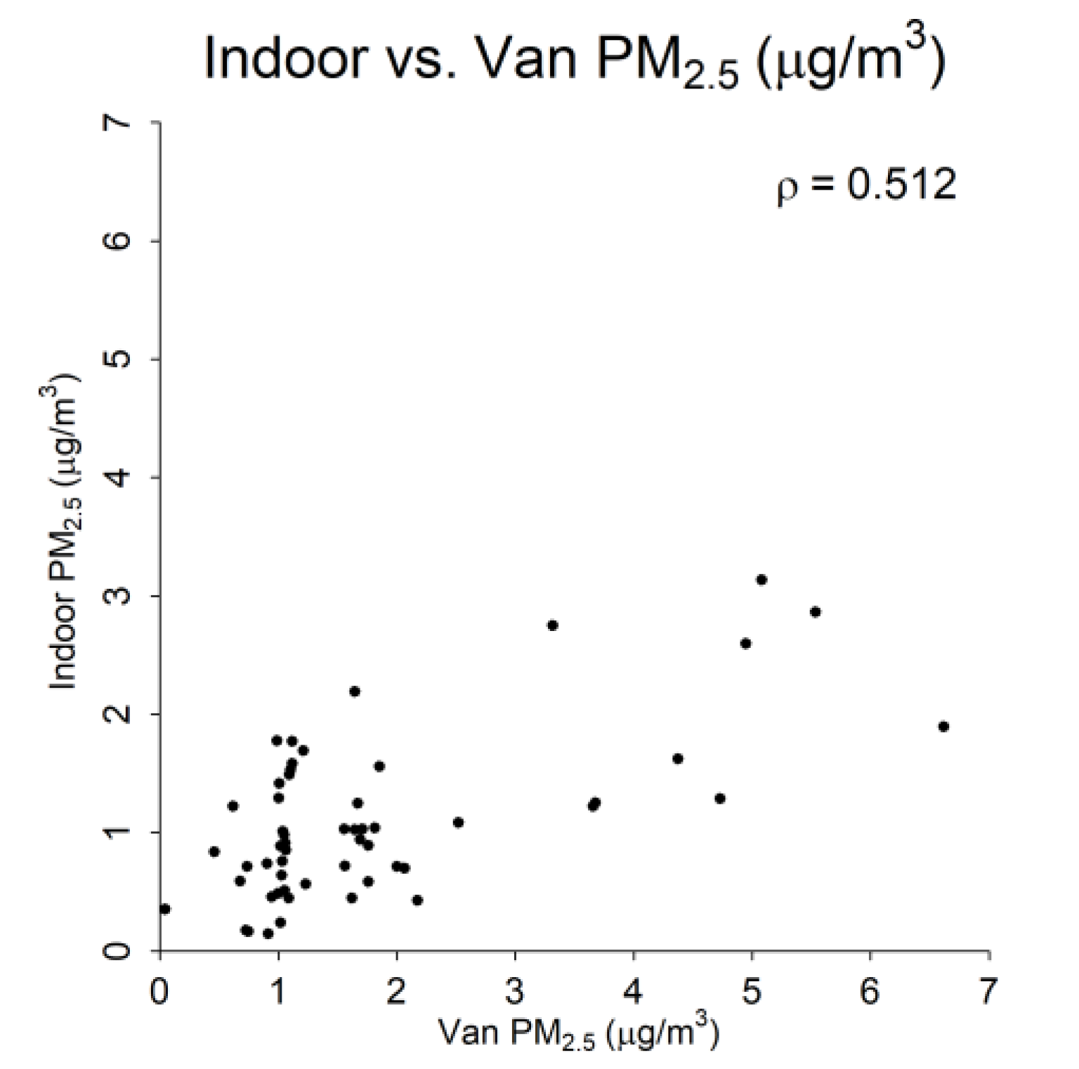
3.1.3. Measurement Site Comparison

The PM_2.5 comparison between the indoor and van sites is shown in

Table 4. Willow Springs correlation test results for site pollutant readings.

Equipment	ρ (rho)	95% CI	p-Value
Indoor vs. Van PM2.5	0.512	0.281–0.741	8.242 × 10−5

and Figure 5. There were only three days where the van and indoor sensors overlapped (15–17 January 2020) and this led to a limited comparison.

3.2. Bonneville Phase 1

The Bonneville Phase 1 campaign involved the van parked at the main parking lot (Monday 16 September 2019 at 9 a.m. until Friday 20 September 2019 at 3 p.m.) near the school drop-off zone, a PM_2.5 and ozone sensor at the school’s playground (Friday 13 September 2019 at 10 a.m. until Friday 27 September 2019 at 5 p.m.), and an ozone sensor inside the school (Friday 13 September 2020 at 8 a.m. until Friday 27 September 2019 at 1 p.m.).

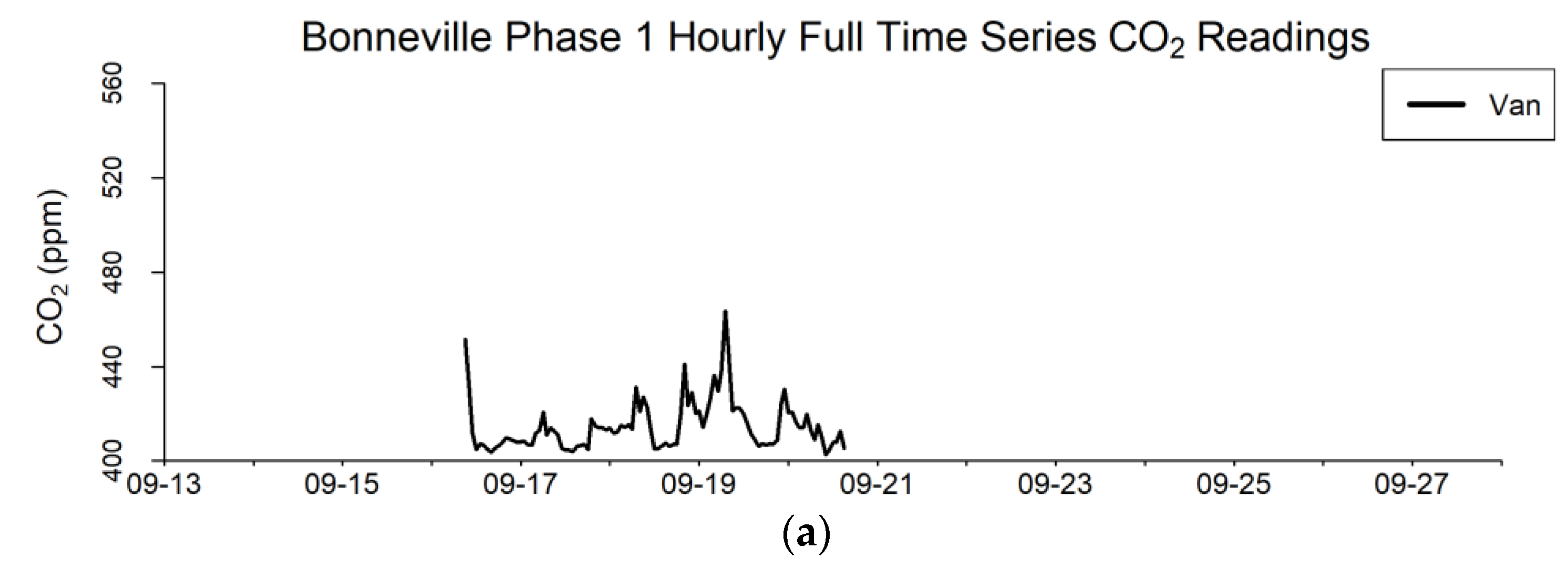
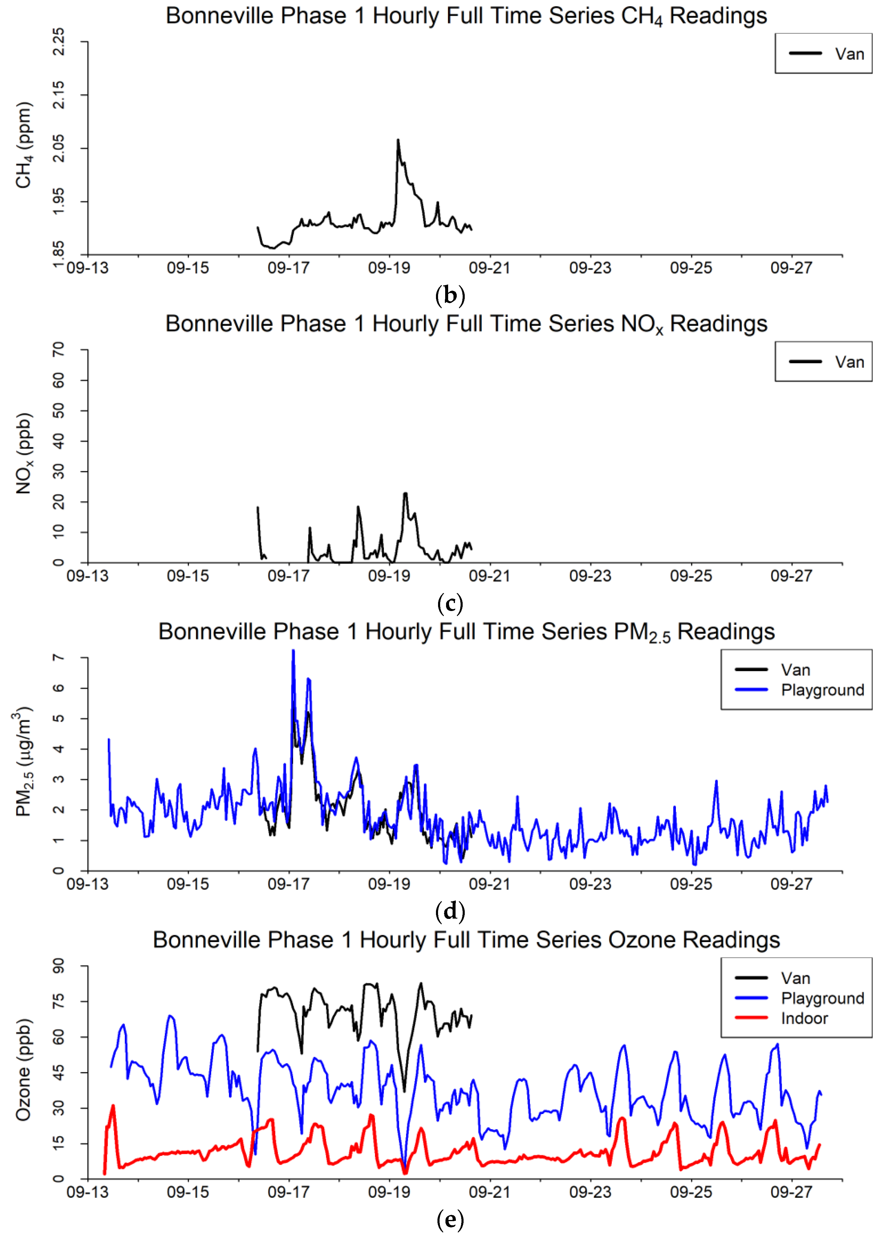
3.2.1. Van Outdoor Pollutant Time Series

The complete time series for the Bonneville Phase 1 campaign for the five study pollutants and three sites is shown in Figure 6. Like the Willow Springs campaign, CO₂, CH₄, NO_x, and PM_2.5 exhibit similar temporal patterns (Figure 6a–d). These four pollutants show a clear peak during the morning rush hour of Thursday, September 19. However, only PM_2.5 has both morning and afternoon rush hour peaks on Tuesday, 17 September (Figure 6d). Furthermore, the playground site shows consistently higher PM_2.5 values than the van, and this is more clearly seen on Tuesday, September 17 (Figure 6d). September is well within high ozone season and the regular diurnal pattern is shown in Figure 6e. The van readings are higher than the playground readings and the indoor readings are the lowest (Figure 6e). The lowest ozone values (Figure 6e) are during the peak NO_x periods (Figure 6c), as expected due to NO_x titration effects.

The weekend readings (14–15 and 21–22 September) show substantially different patterns for indoor and outdoor ozone. This is likely due to the different ventilation schedules for the buildings as they are unoccupied during weekends.

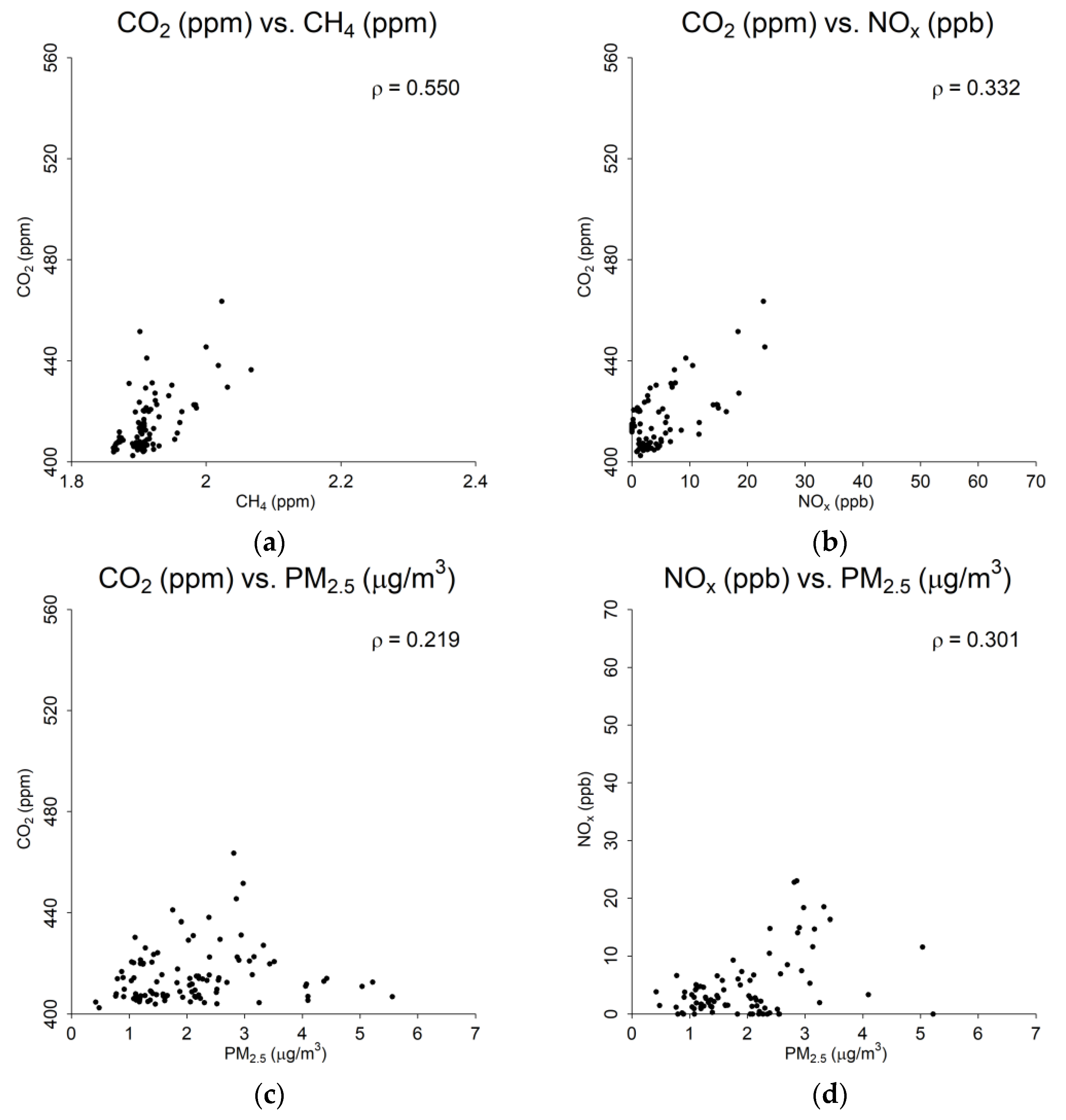
3.2.2. Van Outdoor Pollutant Comparison

The van pollutant comparisons are shown in

Table 5. Bonneville Phase 1 Spearman correlation test results for van pollutant readings.

Equipment	ρ (rho)	95% CI	p-Value
CO2 vs. CH4	0.550	0.393–0.707	2.743 × 10−9
CO2 vs. NOx	0.332	0.126–0.537	0.002
CO2 vs. PM2.5	0.219	0.028–0.410	0.026
NOx vs. PM2.5	0.301	0.065–0.536	0.005

and Figure 7.

Table 5 demonstrates the resulting ρ (Spearman rho) values are substantially lower than those obtained during the Willow Springs campaign. Furthermore, the p-values are overall less statistically significant than those found on Table 2; however, they are all still statistically significant to at least the 0.01 level. The strongest correlation was for CO₂ and CH₄ (ρ = 0.550) and all others are 0.332 and below. The most likely explanation for the weak relationship between CO₂ and NO_x is the NO_x titration cycle creating ozone during this early Fall period. Lastly, the PM_2.5 data are out of sync with the rest of the pollutants due to the marked rush hour values on 17 September 2019. The CO₂ values (Figure 7a–c) are much lower than those observed in Figure 4 due to this observation period being in the fall, following the growing season, as opposed to the winter with less biological activity and more emissions due to heating requirements. Additionally, there were no persistent atmospheric inversion events trapping pollutants.

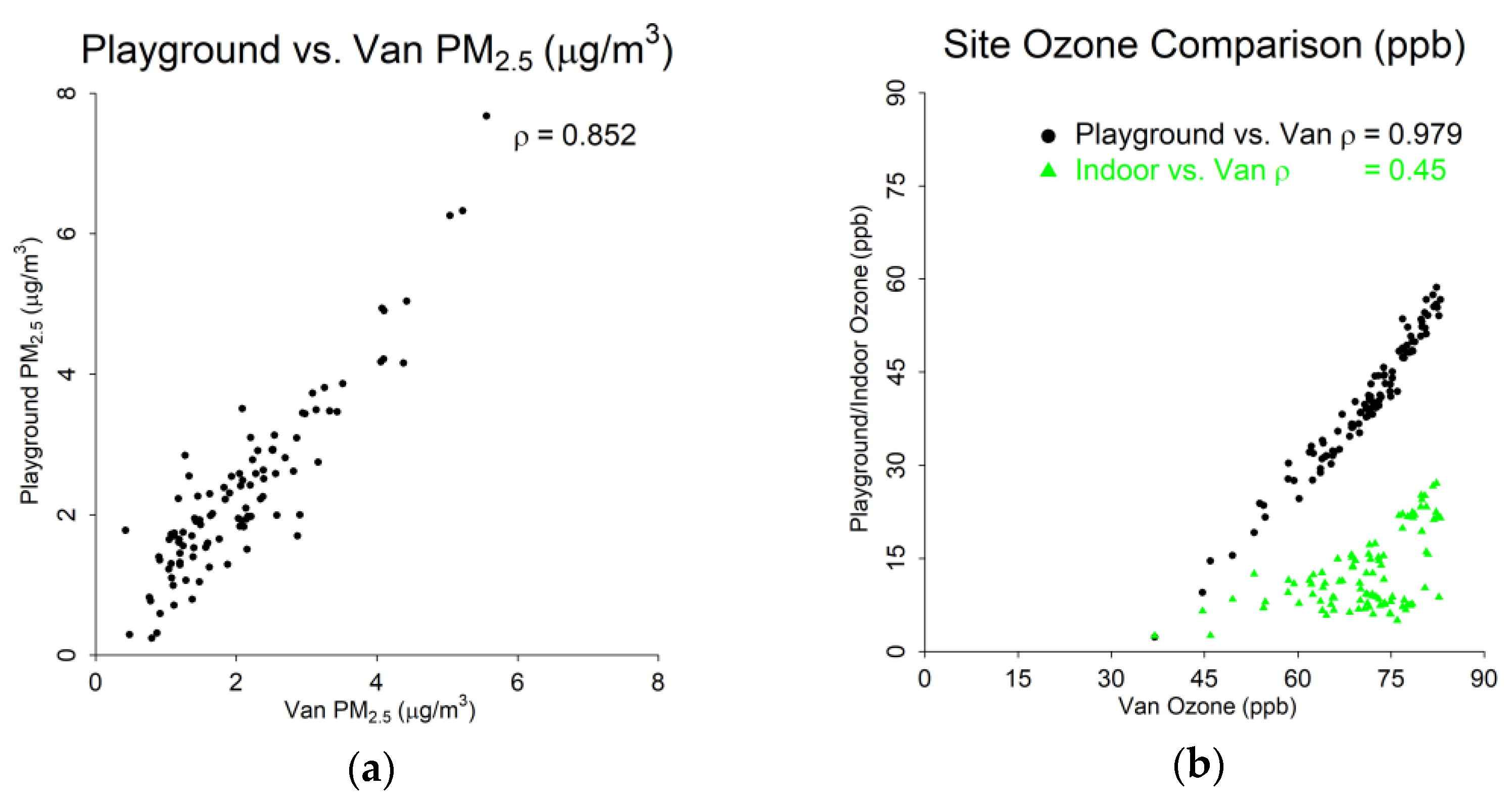
3.2.3. Measurement Site Comparison

The pollutant comparisons between sites are shown in

Table 6. Bonneville Phase 1 Spearman correlation test results for site pollutant readings.

Equipment	ρ (rho)	95% CI	p-Value
Playground vs. Van PM2.5	0.852	0.781–0.922	<2.2 × 10−16
Playground vs. Van Ozone	0.979	0.970–0.988	<2.2 × 10−16
Indoor vs. Van Ozone	0.428	0.240–0.615	6.633 × 10−6
Indoor vs. Playground Ozone	0.493	0.402–0.584	<2.2 × 10−16

and Figure 8. The highest correlations are between van and playground PM_2.5 and ozone (Figure 8a,b). The relationships are much weaker between the van (and playground) and indoor ozone. All these relationships are statistically significant with p-values well below 0.001.

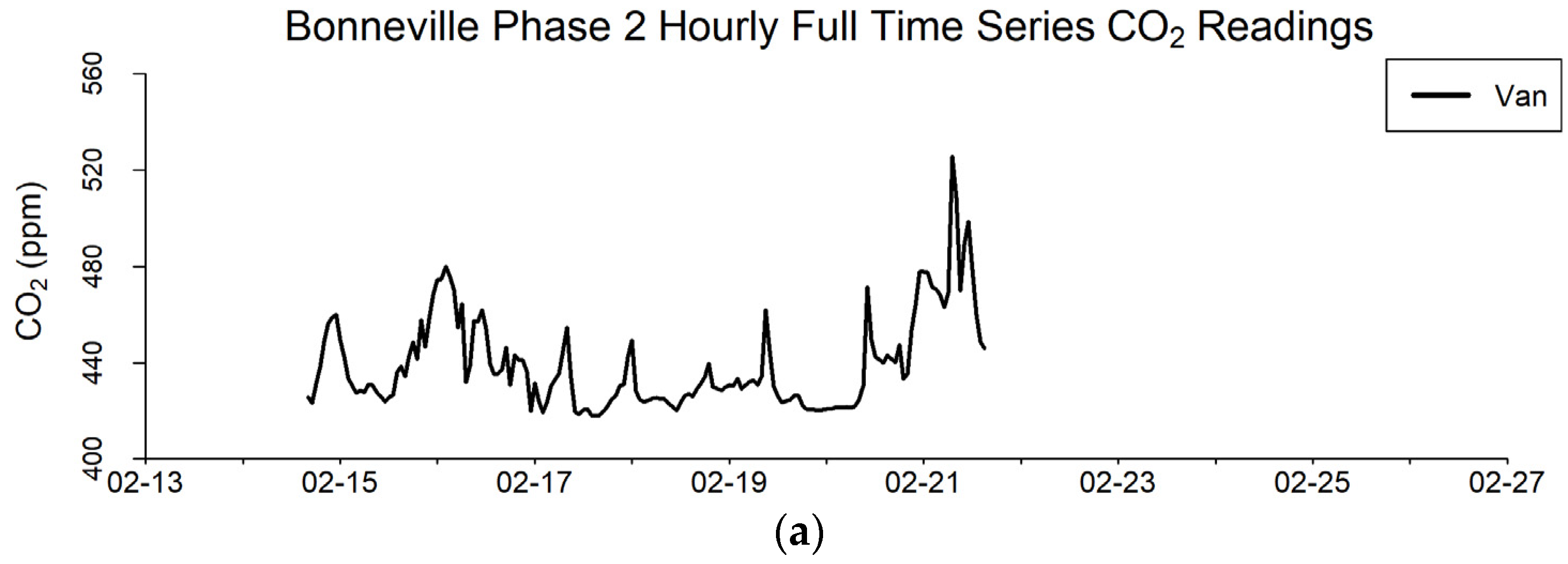
3.3. Bonneville Phase 2

The Bonneville Phase 2 campaign involved three sensors. First, the van parked at the main parking lot (Friday, 14 February 2020 at 4 p.m. until Friday, 21 February 2020 at 3 p.m.) near the school drop-off zone. Second, a PM_2.5 and ozone sensor were placed at the school’s playground (Thursday, 13 February 2020 at 10 a.m. until Wednesday, 26 February 2020 at 4 p.m.). Third, an ozone sensor was placed inside the school (Friday, 21 February 2020 at 4 p.m. until Wednesday, 26 February 2020 at 4 p.m.).

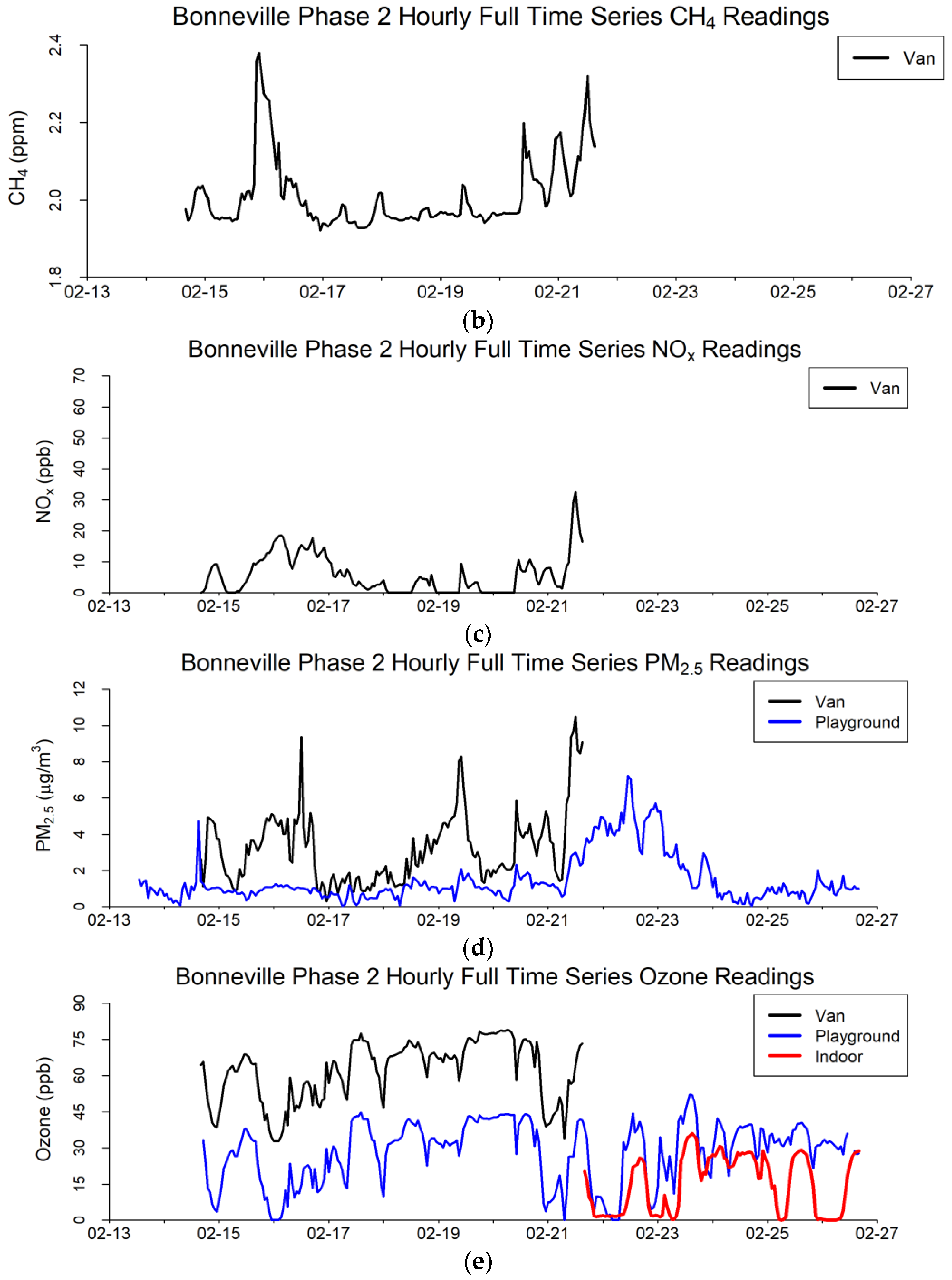
3.3.1. Van Outdoor Pollutant Time Series

The complete time series for the Bonneville Phase 2 campaign for the five study pollutants and three sites is shown in Figure 9. CO₂, CH₄, NO_x, and PM_2.5 show similar patterns (Figure 9a–d), while ozone exhibits a diurnal cycle very similar to the Fall results from the Bonneville Phase 1 campaign described in Section 3.2 (Figure 9e). PM_2.5 was much higher in the van compared to the playground with the morning and afternoon peaks accentuated (Figure 9d). The van also had much higher ozone readings than the playground, and the playground readings were also higher than the indoor readings (Figure 9e).

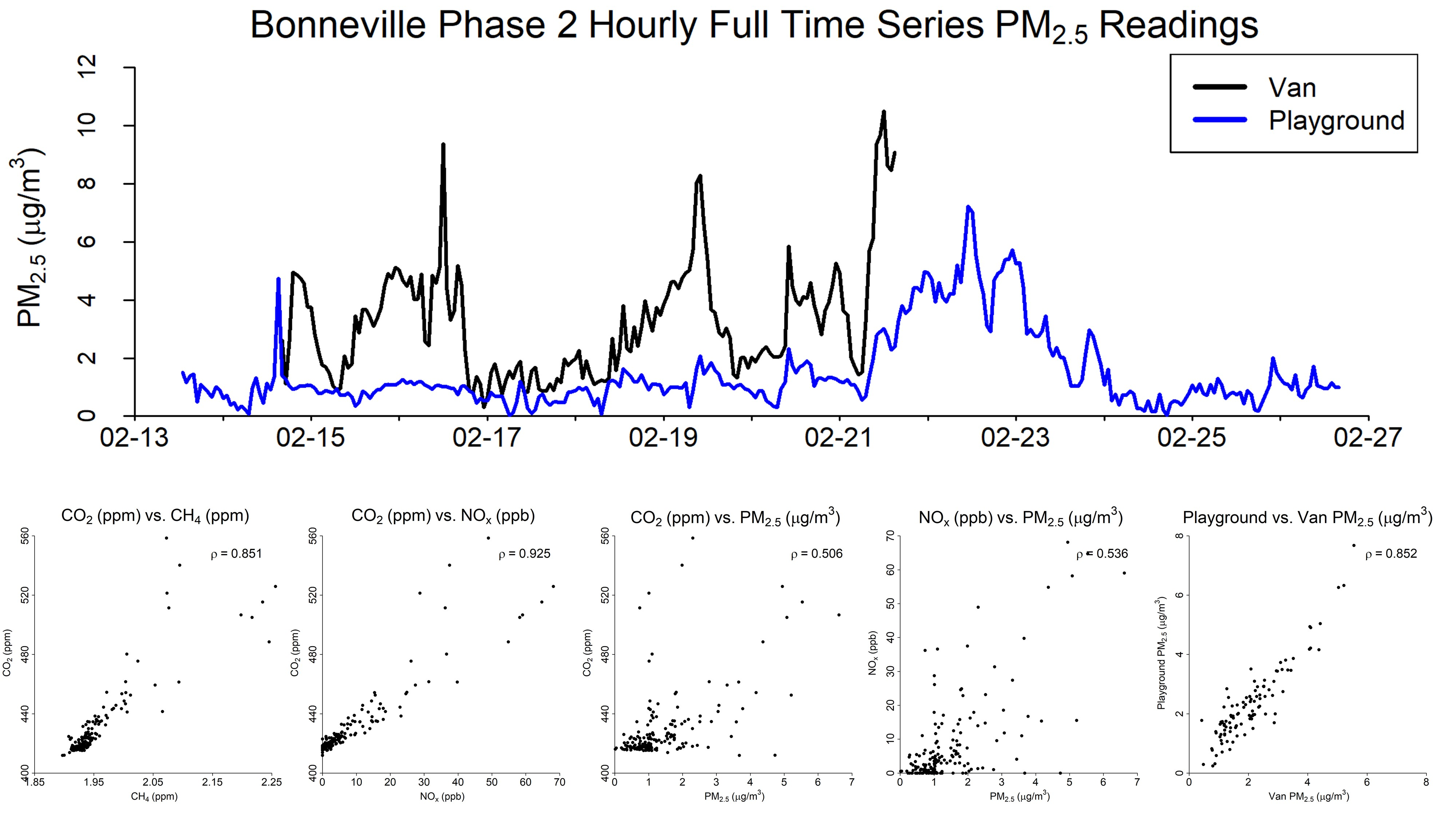
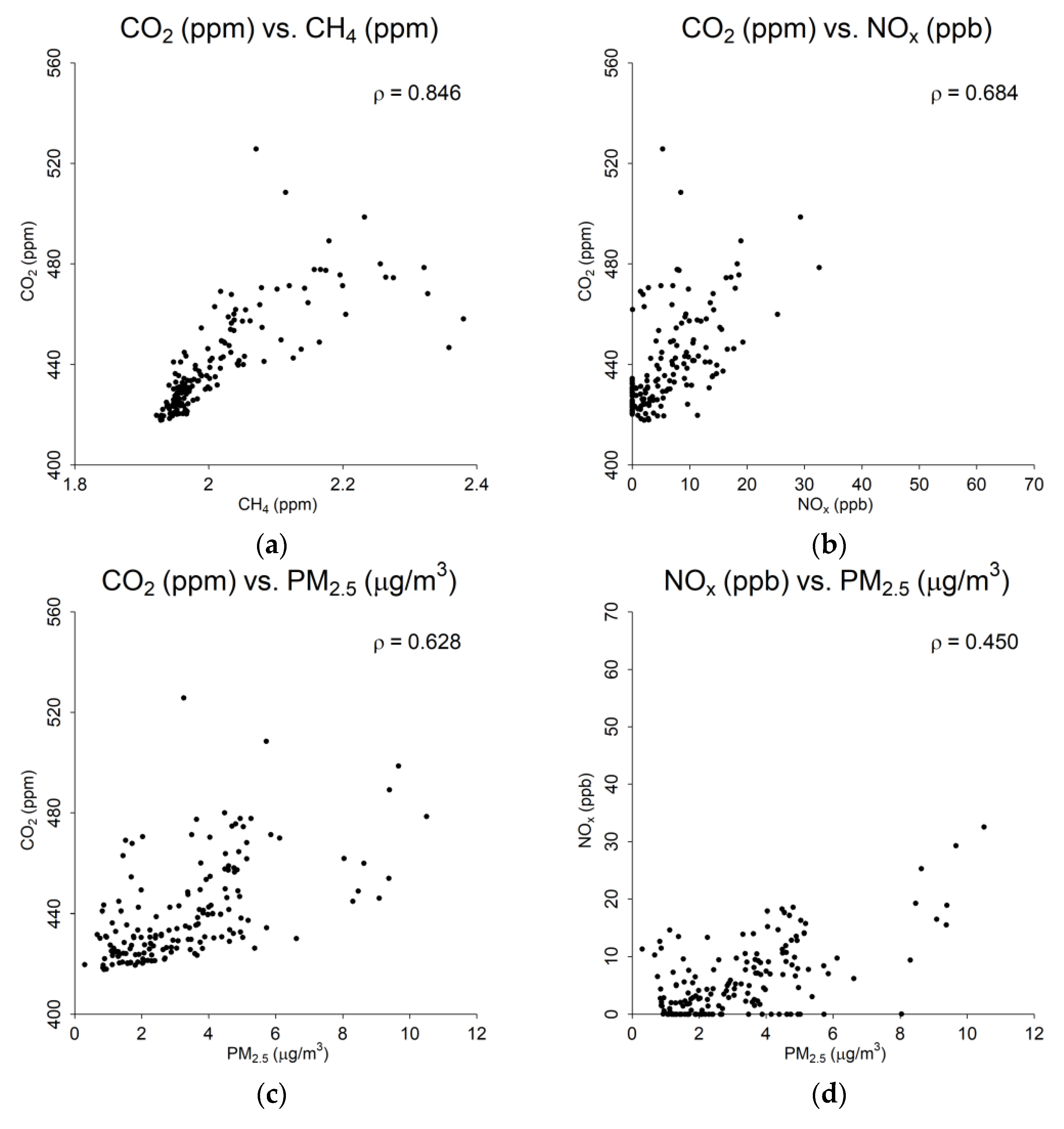
3.3.2. Van Outdoor Pollutant Comparison

The van pollutant comparisons are shown in

Table 7. Bonneville Phase 2 Spearman correlation test results for van pollutant readings.

Equipment	ρ (rho)	95% CI	p-Value
CO2 vs. CH4	0.846	0.792–0.899	<2.2 × 10−16
CO2 vs. NOx	0.684	0.602–0.766	<2.2 × 10−16
CO2 vs. PM2.5	0.628	0.528–0.729	<2.2 × 10−16
NOx vs. PM2.5	0.450	0.306–0.594	9.184 × 10−10

and Figure 10. The strongest correlation was once again between CO₂ and CH₄ (ρ = 0.846) with moderate correlations between CO₂ and NO_x as well as between CO₂ and PM_2.5. The NO_x titration cycle may influence the NO_x concentrations. Furthermore, the high PM_2.5 levels associated with morning rush hour lead to a different concentration pattern than the other pollutants. All these relationships are statistically significant with p-values well below 0.001. Figure 10 showed similar patterns as Figure 7 with CH₄ and PM_2.5 reaching higher values most likely due to the inversion event that took place in the middle of the week.

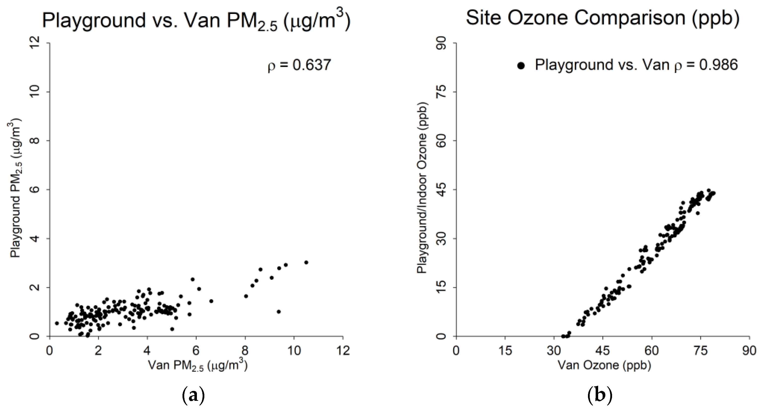
3.3.3. Measurement Site Comparison

The pollutant comparisons between sites are shown in

Table 8. Bonneville Phase 2 Spearman correlation test results for site pollutant readings.

Equipment	ρ (rho)	95% CI	p-Value
Playground vs. Van PM2.5	0.637	0.539–0.735	<2.2 × 10−16
Playground vs. Van Ozone	0.986	0.980–0.992	<2.2 × 10−16
Indoor vs. Playground Ozone	0.606	0.475–0.737	2.749 × 10−13

and Figure 11. The highest correlation is between van and playground and ozone (Figure 11b). Because of the substantial morning rush hour PM_2.5 peaks, which were more noticeable in the van readings than the playground, the correlation between the two is not very high (Figure 11a). There was no overlap between the van and indoor ozone so that relationship is not explored. Furthermore, the correlation between indoor and playground ozone is not very strong (Table 8). All these relationships are statistically significant with p-values well below 0.001.

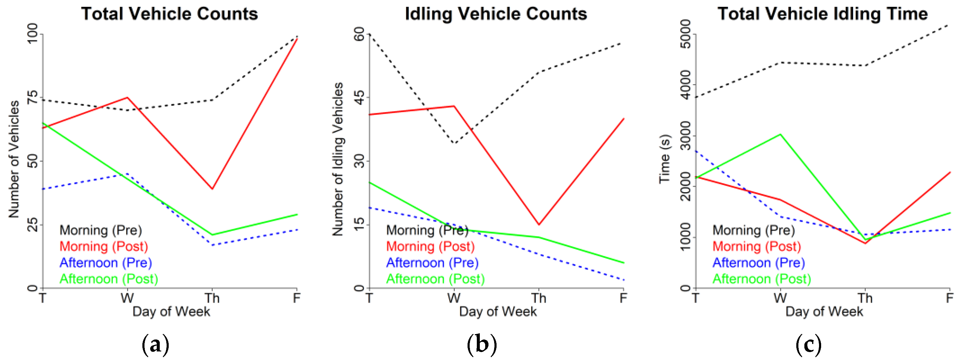
3.4. Bonneville Elementary Idle-Free Campaign Vehicle Counts and Idling Time

The Bonneville Elementary Idle-Free Campaign measurements are shown in

Table 9. Bonneville Elementary Idle-Free Campaign vehicle counts and idling time.

Day of Week		Pre-Campaign			Post-Campaign
		Total Vehicles	Vehicles Idling	Idling Time (s)	Total Vehicles	Vehicles Idling	Idling Time (s)
Tuesday	Morning	74	60	3755	63	41	2195
	Afternoon	39	19	2701	65	25	2166
Wednesday	Morning	70	34	4438	75	43	1738
	Afternoon	45	15	1409	43	14	3027
Thursday	Morning	74	51	4379	39	15	883
	Afternoon	17	8	1058	21	12	956
Friday	Morning	99	58	5193	98	40	2279
	Afternoon	23	2	1152	29	6	1480

and

Table 10. Bonneville Elementary Idle-Free Campaign aggregated and average values.

Time Period		Total Vehicles	Total Idling	Total Idle (s)	Idling (%)	Idling (s/veh)	Idling (s/idler)
Pre-Campaign	Morning	317	203	17,765	64.04	56.04	87.51
	Afternoon	124	44	6320	35.48	50.97	143.64
	Total	441	247	24,085	56.01	54.61	97.51
Post-Campaign	Morning	275	139	7095	50.55	25.80	51.04
	Afternoon	158	57	7629	36.08	48.28	133.84
	Total	433	196	14,724	45.27	34.00	75.12

, and Figure 12. Table 9 and Figure 12 list the total vehicle counts, number of vehicles idling, and aggregated idling time for all idling vehicles. The data are separated by measurement day, morning and afternoon, and pre/post-campaign time period. The pre- and post-campaign counting locations were kept constant for each day to ensure continuity.

Table 10 shows the aggregated and averaged results for the pre- and post-campaign vehicle counts. While the total and idling vehicles counts were greater during post-campaign, the overall idling duration dropped by nearly 39%. Furthermore, the percentage of idling vehicles was almost 11% lower post-campaign. This resulted in markedly lower idling times for the cars that were idling as well as on a per vehicle basis. The most remarkable drop was seen in the morning idling times, which is striking due to the colder temperatures during Phase 2 (February) compared to Phase 1 (September). It is interesting to note that while pre-campaign, the idling times were similar for the morning and afternoon, morning idling times dropped substantially while afternoon idling times stayed relatively constant.

4. Discussion

4.1. Findings

This study sought to explore: (1) inter-pollutant temporal variability, (2) pollutant reading variability between sites within a school, (3) and effects of an anti-idling campaign on pollutant concentrations. It is important to keep in mind that testing the impacts of air pollution emissions campaigns in locations that experience episodic events is complicated due to the strong spatial variability in atmospheric forcing and stagnation that are independent of the emissions themselves. Atmospheric inversion events occurred during the two wintertime campaigns (Willow Springs and Bonneville Phase 2), and they had a substantial impact on the observations.

The inter-pollutant variability (1), using sensors installed on a parked mobile platform, showed a strong seasonal dependence. This seasonal dependence was particularly true for CO₂, NO_x, and ozone due to seasonal changes in ozone formation rates. Furthermore, persistent atmospheric inversion events lead to substantial pollutant accumulation and formation of secondary PM_2.5, which lead to divergences in pollutant temporal signatures. It seems that the van’s ozone sensors may have a positive offset for the two Bonneville campaigns; however, this would not impact the slope, simply the intersect of the relationships.

The site variability (2) showed much stronger correlation between outdoor ozone values recorded at the van and on the school playground compared to indoor and outdoor ozone values. Building ventilation schedules are likely the main contributors to the differences between indoor and outdoor ozone. Outdoor PM_2.5 values had a substantially lower correlation during persistent inversion episodes compared to the non-inversion periods. All these relationships were found to be statistically significant.

The impact of anti-idling campaigns on pollutant concentrations (3) was less clear cut in terms of pollution decrease. The Bonneville Phase 2 campaign had an inversion event in the middle of this study, thus making it difficult to ascertain the impact of the effort to reduce idling. Due to the short campaign periods, as well as lack of sensor overlap across the measurement sites, these results should be considered preliminary, but encouraging. However, there were measurable reductions in idling behavior that support development and implementation of future anti-idling efforts. Although February (post-campaign) is typically colder than September (pre-campaign), cars idled less on average and a smaller fraction of cars idled despite the potential comfort implications.

4.2. Implications

Findings such as those presented here are important because they illustrate the value of idling campaigns in schools. Since many schools are bordering major roadways or highways, and since parents increasingly drop children at school, understanding inter-pollutant and spatial variability can help protect children in school settings [34,35]. Reduced pollutants due to this behavior shift can also benefit schoolteachers and staff and improve local air quality. While further research will need to be performed to verify our results presented here, there is a growing body of research that supports our findings. Moreover, idling campaigns are low cost, and the co-benefits of the policies are often also economically beneficial, which adds to the overall benefit of the policy and the continued social norm. These efforts are particularly relevant and effective when they involve the community where the idling occurs, ensuring a better understanding of a behavior and its health benefits.

4.3. Limitations

This study has a few limitations. The length of the study periods is variable, but the timeframe of this study was on the short side. This made this study vulnerable to outside factors such as the resulting inversion events. Additionally, the Bonneville study was conducted over two seasons with substantially different pollutant emission and transport characteristics—early fall and mid-winter. A further complication was that the van recorded data for a week while the playground and indoor sites recorded for longer periods of time. In the case of Bonneville Phase 2, the van’s data record did not intersect at all with the indoor site. It was also discovered that the van’s ozone sensor had a positive bias during both phases of the Bonneville campaign.

4.4. Future Work

This pilot anti-idling campaign is a starting point to develop arguments for more effective and precise control of vehicular idling during school drop-off and pick-up times. Future studies will take longer measurements (2–3 weeks) as well as include indoor PM_2.5 sensors. Additionally, follow-up studies will need to revisit sample schools during the same season to understand whether anti-idling behavior campaigns had a lasting effect or if parents reduced their idling behavior only when actively asked to.

5. Conclusions

This research aimed to assess the effectiveness of two anti-idling campaigns in Salt Lake County, Utah. The goal of this study was to understand if reduced engine idling leads to the subsequent reduction in traffic-related air pollution exposure of the related school communities. Seasonal variability and atmospheric inversion events affected air quality readings but modest improvements in air quality were found in the middle of the campaign. The 38% decrease in idling time and 11% decrease in the number of vehicles idling at the school drop-off zones following an anti-idling campaign provide the justification for additional anti-idling campaigns to protect the health of children, school staff, and the surrounding community.

References

1. Carrico, A.R.; Padgett, P.; Vandenbergh, M.P.; Gilligan, J.; Wallston, K.A. Costly myths: An analysis of idling beliefs and behavior in personal motor vehicles. Energy Policy 2009, 37, 2881–2888. [Google Scholar] [CrossRef]
2. Lee, Y.-Y.; Lin, S.-L.; Aniza, R.; Yuan, C.-S. Reduction of Atmospheric PM2.5 Level by Restricting the Idling Operation of Buses in a Busy Station. Aerosol Air Qual. Res. 2017, 17, 2424–2437. [Google Scholar] [CrossRef] [Green Version]
3. Kinsey, J.S.; Williams, D.C.; Dong, Y.; Logan, R. Characterization of Fine Particle and Gaseous Emissions during School Bus Idling. Environ. Sci. Technol. 2007, 41, 4972–4979. [Google Scholar] [CrossRef] [PubMed]
4. Breton, C.V.; Mack, W.J.; Yao, J.; Berhane, K.; Amadeus, M.; Lurmann, F.; Gilliland, F.; McConnell, R.; Hodis, H.N.; Kunzli, N.; et al. Prenatal Air Pollution Exposure and Early Cardiovascular Phenotypes in Young Adults. PLoS ONE 2016, 11, e0150825. [Google Scholar] [CrossRef]
5. Zhang, X.; Chen, X.; Zhang, X. The impact of exposure to air pollution on cognitive performance. Proc. Natl. Acad. Sci. USA 2018, 115, 9193–9197. [Google Scholar] [CrossRef] [Green Version]
6. Vishnevetsky, J.; Tang, D.; Chang, H.-W.; Roen, E.L.; Wang, Y.; Rauh, V.; Wang, S.; Miller, R.L.; Herbstman, J.; Perera, F.P. Combined effects of prenatal polycyclic aromatic hydrocarbons and material hardship on child IQ. Neurotoxicol. Teratol. 2015, 49, 74–80. [Google Scholar] [CrossRef] [PubMed] [Green Version]
7. Barnes, N.M.; Ng, T.W.; Ma, K.K.; Lai, K.M. In-Cabin Air Quality during Driving and Engine Idling in Air-Conditioned Private Vehicles in Hong Kong. Int. J. Environ. Res. Public Health 2018, 15, 611. [Google Scholar] [CrossRef] [Green Version]
8. Keyvanfar, A.; Shafaghat, A.; Muhammad, N.Z.; Ferwati, M.S. Driving Behaviour and Sustainable Mobility—Policies and Approaches Revisited. Sustainability 2018, 10, 1152. [Google Scholar] [CrossRef] [Green Version]
9. Kim, J.Y.; Ryan, P.H.R.; Yermakov, M.; Schaffer, C.; Reponen, T.; Grinshpun, S.A. The Effect of an Anti-idling Campaign on Indoor Aerosol at Urban Schools. Aerosol Air Qual. Res. 2014, 14, 585–595. [Google Scholar] [CrossRef] [Green Version]
10. Lee, Y.-Y.; Lin, S.-L.; Yuan, C.-S.; Lin, M.-Y.; Chen, K.-S. Reduction of atmospheric fine particle level by restricting the idling vehicles around a sensitive area. J. Air Waste Manag. Assoc. 2018, 68, 656–670. [Google Scholar] [CrossRef] [Green Version]
11. Macneill, M.; Dobbin, N.; St-Jean, M.; Wallace, L.; Marro, L.; Shin, T.; You, H.; Kulka, R.; Allen, R.W.; Wheeler, A.J. Can changing the timing of outdoor air intake reduce indoor concentrations of traffic-related pollutants in schools? Indoor Air 2016, 26, 687–701. [Google Scholar] [CrossRef] [PubMed]
12. Abrams, D.; Lalot, F.; Hopthrow, T.; Templeton, A.; Steeden, B.; Özkeçeci, H.; Imada, H.; Warbis, S.; Sandiford, D.; Meleady, R.; et al. Cleaning up our acts: Psychological interventions to reduce engine idling and improve air quality. J. Environ. Psychol. 2021, 74, 101587. [Google Scholar] [CrossRef]
13. Danek, T.; Zaręba, M. The Use of Public Data from Low-Cost Sensors for the Geospatial Analysis of Air Pollution from Solid Fuel Heating during the COVID-19 Pandemic Spring Period in Krakow, Poland. Sensors 2021, 21, 5208. [Google Scholar] [CrossRef] [PubMed]
14. Tudor, C.; Sova, R. EU Net-Zero Policy Achievement Assessment in Selected Members through Automated Forecasting Algorithms. ISPRS Int. J. Geo-Inf. 2022, 11, 232. [Google Scholar] [CrossRef]
15. Lynn, J.; Oppenheimer, S.; Zimmer, L. Using public policy to improve outcomes for asthmatic children in schools. J. Allergy Clin. Immunol. 2014, 134, 1238–1244. [Google Scholar] [CrossRef]
16. American Lung Association. State of the Air 2021; American Lung Association: Washington, DC, USA, 2021. [Google Scholar]
17. INRIX Research. INRIX Global Traffic Score Card; INRIX: Irvine, CA, USA, 2020. [Google Scholar]
18. Horel, J.; Crosman, E.; Jacques, A.; Blaylock, B.; Arens, S.; Long, A.; Sohl, J.; Martin, R. Summer ozone concentrations in the vicinity of the Great Salt Lake. Atmos. Sci. Lett. 2016, 17, 480–486. [Google Scholar] [CrossRef]
19. Whiteman, C.D.; Hoch, S.W.; Horel, J.D.; Charland, A. Relationship between particulate air pollution and meteorological variables in Utah’s Salt Lake Valley. Atmos. Environ. 2014, 94, 742–753. [Google Scholar] [CrossRef]
20. Mendoza, D.L.; Benney, T.M.; Boll, S. Long-term analysis of the relationships between indoor and outdoor fine particulate pollution: A case study using research grade sensors. Sci. Total Environ. 2021, 776, 145778. [Google Scholar] [CrossRef]
21. Mendoza, D.; Crosman, E.; Mitchell, L.; Jacques, A.; Fasoli, B.; Park, A.; Lin, J.; Horel, J. The TRAX Light-Rail Train Air Quality Observation Project. Urban Sci. 2019, 3, 108. [Google Scholar] [CrossRef] [Green Version]
22. Bulot, F.M.J.; Russell, H.S.; Rezaei, M.; Johnson, M.S.; Ossont, S.J.J.; Morris, A.K.R.; Basford, P.J.; Easton, N.H.C.; Foster, G.L.; Loxham, M.; et al. Laboratory Comparison of Low-Cost Particulate Matter Sensors to Measure Transient Events of Pollution. Sensors 2020, 20, 2219. [Google Scholar] [CrossRef] [Green Version]
23. Bush, S.E.; Hopkins, F.M.; Randerson, J.T.; Lai, C.-T.; Ehleringer, J.R. Design and application of a mobile ground-based observatory for continuous measurements of atmospheric trace gas and criteria pollutant species. Atmos. Meas. Tech. 2015, 8, 3481–3492. [Google Scholar] [CrossRef] [Green Version]
24. Hopkins, F.M.; Kort, E.; Bush, S.E.; Ehleringer, J.R.; Lai, C.-T.; Blake, D.R.; Randerson, J.T. Spatial patterns and source attribution of urban methane in the Los Angeles Basin. J. Geophys. Res. Atmos. 2016, 121, 2490–2507. [Google Scholar] [CrossRef]
25. 2B Technologies, Inc. Ozone Monitor Operation Manual Model 205; 2B Technologies: Boulder, CO, USA, 2018. [Google Scholar]
26. ES-642 Dust Monitor Operation Manual; Met One Instruments, Inc.: Pass, OR, USA, 2013.
27. Mitchell, L.E.; Crosman, E.T.; Jacques, A.A.; Fasoli, B.; Leclair-Marzolf, L.; Horel, J.; Bowling, D.R.; Ehleringer, J.R.; Lin, J.C. Monitoring of greenhouse gases and pollutants across an urban area using a light-rail public transit platform. Atmos. Environ. 2018, 187, 9–23. [Google Scholar] [CrossRef]
28. Google Maps. Available online: https://www.google.com/maps (accessed on 22 November 2018).
29. USGS TNM Elevation Tool. Available online: https://apps.nationalmap.gov/elevation/ (accessed on 20 April 2022).
30. Utah Division of Air Quality. Utah Division of Air Quality 2020 Annual Report; Utah Division of Air Quality: Salt Lake City, UT, USA, 2021.
31. Utah Division of Air Quality. 2017 Emissions Data Provided in Tons/Year; Utah Division of Air Quality: Salt Lake City, UT, USA, 2020.
32. Lareau, N.P.; Crosman, E.; Whiteman, C.D.; Horel, J.D.; Hoch, S.W.; Brown, W.O.; Horst, T.W. The persistent cold-air pool study. Bull. Am. Meteorol. Soc. 2013, 94, 51–63. [Google Scholar] [CrossRef] [Green Version]
33. Bares, R.; Lin, J.C.; Hoch, S.W.; Baasandorj, M.; Mendoza, D.L.; Fasoli, B.; Mitchell, L.; Catharine, D.; Stephens, B.B. The Wintertime Covariation of CO 2 and Criteria Pollutants in an Urban Valley of the Western United States. J. Geophys. Res. Atmos. 2018, 123, 2684–2703. [Google Scholar] [CrossRef]
34. Mullen, C.; Grineski, S.E.; Collins, T.W.; Mendoza, D.L. Effects of PM2.5 on Third Grade Students’ Proficiency in Math and English Language Arts. Int. J. Environ. Res. Public Health 2020, 17, 6931. [Google Scholar] [CrossRef]
35. Mendoza, D.L.; Pirozzi, C.S.; Crosman, E.T.; Liou, T.G.; Zhang, Y.; Cleeves, J.J.; Bannister, S.C.; Anderegg, W.R.; Paine, R., III. Impact of low-level fine particulate matter and ozone exposure on absences in K-12 students and economic consequences. Environ. Res. Lett. 2020, 15, 114052. [Google Scholar] [CrossRef]
Figure 1. Salt Lake City and Salt Lake County within Utah and the United States (left inset) with the interstate highways (I-15, I-80, I-215) noted.
Atmosphere 13 00706 g001
Figure 2. Study area showing the instrument locations at (a) Willow Springs Elementary and (b) Bonneville Elementary. The parking location of the van is denoted by a yellow star, the playground site is marked by a red circle, and the approximate location of the indoor site is marked by a blue sign. Images courtesy of Google Maps.
Atmosphere 13 00706 g002
Figure 3. Time series (tick mark denotes midnight) for Willow Springs campaign (10–17 January 2020) for (a) carbon dioxide, (b) methane, (c) nitrogen oxides, (d) fine particulate matter, and (e) ozone.
Atmosphere 13 00706 g003aAtmosphere 13 00706 g003b
Figure 4. Van pollutant readings comparisons for Willow Springs campaign (10–17 January 2020) for (a) carbon dioxide vs. methane, (b) carbon dioxide vs. nitrogen oxides, (c) carbon dioxide vs. fine particulate matter, and (d) nitrogen oxides vs. fine particulate matter.
Atmosphere 13 00706 g004
Figure 5. Site pollutant readings comparisons for Willow Springs campaign (10–28 January 2020) for fine particulate matter.
Atmosphere 13 00706 g005
Figure 6. Time series (tick mark denotes midnight) for Bonneville Phase 1 campaign (13–27 September 2019) for (a) carbon dioxide, (b) methane, (c) nitrogen oxides, (d) fine particulate matter, and (e) ozone.
Atmosphere 13 00706 g006aAtmosphere 13 00706 g006b
Figure 7. Van pollutant readings comparisons for Bonneville Phase 1 campaign (13–27 September 2019) for (a) carbon dioxide vs. methane, (b) carbon dioxide vs. nitrogen oxides, (c) carbon dioxide vs. fine particulate matter, and (d) nitrogen oxides vs. fine particulate matter.
Atmosphere 13 00706 g007
Figure 8. Site pollutant readings comparisons for Bonneville Phase 1 campaign (13–27 September 2019) for (a) fine particulate matter and (b) ozone.
Atmosphere 13 00706 g008
Figure 9. Time series (tick mark denotes midnight) for Bonneville Phase 2 campaign (13–27 February 2020) for (a) carbon dioxide, (b) methane, (c) nitrogen oxides, (d) fine particulate matter, and (e) ozone.
Atmosphere 13 00706 g009aAtmosphere 13 00706 g009b
Figure 10. Van pollutant readings Bonneville Phase 2 campaign (13–27 February 2020) for (a) carbon dioxide vs. methane, (b) carbon dioxide vs. nitrogen oxides, (c) carbon dioxide vs. fine particulate matter, and (d) nitrogen oxides vs. fine particulate matter.
Atmosphere 13 00706 g010
Figure 11. Site pollutant readings comparisons for Bonneville Phase 2 campaign (13–27 February 2020) for (a) fine particulate matter and (b) ozone.
Atmosphere 13 00706 g011
Figure 12. Weekday time of day pre- and post-campaign: (a) total vehicle counts, (b) idling vehicle counts, and (c) total vehicle idling time.
Atmosphere 13 00706 g012