Article

GAN-rcLSTM: A Deep Learning Model for Radar Echo Extrapolation

1
School of Computer and Software, Nanjing University of Information Science and Technology, Nanjing 210044, China
2
Jiangsu Meteorological Observatory, Nanjing 210008, China
*
Author to whom correspondence should be addressed.
Atmosphere 2022, 13(5), 684; https://doi.org/10.3390/atmos13050684
Submission received: 2 March 2022 / Revised: 15 April 2022 / Accepted: 20 April 2022 / Published: 24 April 2022

Abstract

:
The target of radar echo extrapolation is to predict the motion and development of radar echo in the future based on historical radar observation data. For such spatiotemporal prediction problems, a deep learning method based on Long Short-Term Memory (LSTM) networks has been widely used in recent years, although such models generally suffer from weak and blurry prediction. This paper proposes two models called Residual Convolution LSTM (rcLSTM) and Generative Adversarial Networks-rcLSTM (GAN-rcLSTM): The former introduces the residual module, and the latter introduces the discriminator. We use the historical data of 2017 and 2018 in the Jiangsu region as training and test sets. Experiments show that in long sequence forecasts, our model can provide more stable and clear images, while achieving higher CSI scores.

1. Introduction

An accurate weather forecast system can greatly reduce the economic losses caused by natural disasters. According to the period validity, as shown in the Table 1, forecast types can be divided into nowcasting, short-term forecasting, short-range forecasting, medium-range forecasting, and long-range forecasting. At present, the forecasting methods can be mainly divided into two categories: One is the Numerical Weather Prediction (NWP) method, and the other is the extrapolation method based on the radar echo. The NWP methods take the spatial distribution of meteorological elements at a certain time as the initial value, establish a complex physical state equation under given boundary conditions, and simulate the atmospheric movement in the future through a large computer. The NWP methods are very mature in short-range and medium-range forecasting operations. However, due to the complexity of the solution process of the differential equation system, NWP methods have the problems of prediction delay and low resolution. Therefore, extrapolation methods based on radar echoes are more widely used in short-term and nowcasting operations (0–12 h). A radar echo sequence contains a lot of information, from which we can analyze the intensity, location, and movement of typhoons, thunderstorms, rainstorms, squall lines, hail, tornadoes, and other disastrous weather. The target of radar extrapolation is to predict the future fixed length radar echo map of a region based on the previously observed radar echo map.
At present, the traditional extrapolation methods are mainly centroid tracking [1,2], cross-correlation [3,4], and optical flow [5,6,7,8,9,10]. The cross correlation method divides the whole data area into several small areas, and then calculates the correlation coefficient between the small areas of the radar echo image at adjacent times. The average motion of the echo region is determined by the correlation between regions. However, in severe convective weather, tracking failure will increase significantly. The optical flow method calculates the instantaneous velocity field of the pixel movement on the target surface by making two basic assumptions (constant brightness and small moving distance of the target), and then predicts the next frame image. The advantage of the optical flow method is that it can detect and identify the position of the moving target without knowing the information of the scene. The optical flow method makes two basic assumptions: The image brightness is constant, and the moving distance of the target is small. The next frame image is predicted by calculating the instantaneous velocity field of pixel motion on the target surface. The advantage of optical flow method is that it can detect and identify the position of moving targets without understanding the scene information, but the computational cost is too high to meet the needs of high-resolution real-time prediction.
In recent years, deep-learning-based models have made great progress in the field of spatiotemporal prediction [11,12,13,14,15,16,17,18,19,20,21]. Because spatiotemporal prediction is a sequence to sequence problem, Recurrent Neural Network (RNN) [22] and its variants, Long short-term memory (LSTM) [23] and Gate Recurrent Unit (GRU) [24], have been widely used. The LSTM model uses a ‘gate’ structure to control the flow of information and avoid the disappearance of gradient in RNN. LSTM has three gates in total, including the input gate, forget gate, and output gate. The forget gate controls how many cell states are discarded at the last moment. The input gate controls how much new information will enter the current cell state. Finally, the output gate determines which parts of the cell state need to be output. Each gate consists of a full connection layer and a sigmoid function. The current time input signal x t and the previous time hidden layer output h t 1 determine the size of the gate. Zero stands for “filter all information”, and one stands for “pass all information”. RNN, LSTM, and GRU all use full connection operations in input-to-state and state-to-state. Srivastava [25] applied LSTM and a self-coding mechanism to video prediction. One LSTM is used as an encoder to extract the feature of the input sequence, and the other LSTM copies the state of the encoder and circularly predicts the subsequent time as a decoder. Shi [26] proposed ConvLSTM and used it to predict precipitation in Guangdong, Hong Kong, and the Macao Bay area. ConvLSTM uses convolution operation instead of full connection operation, which gives LSTM the ability to extract spatial features and greatly reduce the number of network parameters. Xu [27] proposed a dynamic convolution network, which generates a convolution kernel for each input through a generator. The adaptive mechanism of DFN makes the model more robust. Shi [28] proposed TrajGRU using the idea of dynamic convolution network. This model is more flexible than convGRU with fixed connection structure. In addition, aiming at the imbalance problem of low proportion of high precipitation samples in real life, the measurement methods of balanced mean square error (B-MSE) and balanced absolute error (B-MAE) are also proposed. TrajGRU improves the accuracy of the model for predicting problems with imbalanced samples, such as lightning and heavy precipitation. Wang [29,30] extended ConvLSTM and proposed PredRNN and PredRNN++. In addition to the vertically transmitted states C and H, these models also have the zigzag propagation state M, so that the cell can see the information of all layers at the previous time. The basic unit of PredRNN++ is a cascade structure, and the results of State C are used for the calculation of state M. At the same time, inspired by highway [31], a gradient high unit (GHU) similar to the GRU structure is inserted between the first and second layers to alleviate the feature loss of state M in the long-term prediction process. PredRNN and PredRNN++ make the connection between different layers tighter through additional propagation paths but require more gates to control the flow of information, making the model more complex. Wang [32] proposed the Memory In Memory (MIM) networks.Experiments show that the forget gate in the long and short-term memory plays a limited role in the long-term prediction process, so it is replaced by two cascaded mim-n and mim-s. The difference between the two time hidden layers is used as an input to increase the oblique propagation path of the feature. Wang proposed E3DLSTM [33], which replaces the forget gate with the recall gate structure. The recall gate is calculated by multiplying the candidate state R and the State C of multiple times in the past. E3D-LSTM alleviates the problem of forgetting the gate gradient saturation, but the recall gate structure in the model uses matrix multiplication, which greatly increases the computational cost required by the model. Chen [20] proposed a coding prediction model (3DCNN-bcLSTM) combining 3DCNN and bi-directional convolution LSTM. He [19] developed an improved model called M-ConvGRU, which performs convolution operations on the input data and previous output of a GRU network. Geng [21] defined a Multi-Scale Criss-Cross Attention Context Sensing Long Short-Term Memory (MCCS-LSTM). MCCS-LSTM integrates the attention mechanism into ConvLSTM, which improves the model context utilization. Ravuri [34] proposed a probabilistic forecasting model called DGMR to improve the forecasting ability of heavy precipitation weather. DGMR uses convolution to constrain the spatial consistency and temporal consistency of the forecast sequence to produce clear forecasts. In general, ConvLSTM first reduces the number of parameters of LSTM-based deep models to a level that can be operationalized. After that, some research improved ConvLSTM to improve the feature extraction ability, including increasing the gradient propagation route, incorporating an attention mechanism, dynamic convolution, etc. After several years of development, state-of-the-art deep learning models have achieved higher accuracy than traditional methods in the short-term radar extrapolation problem in regular weather.
However, almost all models based on LSTM have two obvious problems. The first is echo decay. Recent evidence shows that stacking layers in an end-to-end fashion enables the network to extract more complex feature patterns, so network depth is critical [35,36,37,38]. However, some studies also reveal that [39,40,41] has a degradation problem in deep networks. As the network depth increases, the model’s score becomes saturated and then drops rapidly. In deep LSTM models, the gradients are difficult to propagate to the bottom layer, and the extrapolation results are always gradually lower than the true value.The second is blur. Usually after an hour, the predicted image will become blurred. Because the traditional LSTM network takes the prediction of the previous time as the input of the next time. This training method does not take the prediction sequence as a whole, but calculates the mean square error hourly and then calculates the average value. During training, the neural network will give a more conservative prediction in order to avoid gradient punishment. In order to solve these two problems, we propose two models: residual convolution LSTM (rcLSTM) and Generative Adversarial Networks-residual convolution LSTM (GAN-rcLSTM).

2. Materials and Methods

The radar echo image transformed by Cartesian coordinate system can be regarded as a gray image, and each pixel value is distributed between 0 and 70. Suppose we express the meteorological data as a dynamical system over time. The observation at any time can be represented by a tensor X R P × M × N , where M × N represents the spatial region, and P is the number of meteorological factors. Then, the prediction of sea surface temperature anomalies can be expressed as an unsupervised spatiotemporal prediction problem, that is, according to a length-J sequence, we can predict the most likely distribution of the sequence after K times in the future:
X ^ t + 1 , , X ^ t + K = arg max X t + 1 , , X t + K p X t + 1 , , X t + K X t J + 1 , , X t

2.1. rcLSTM

Inspired by Resnet [39], which has made great breakthroughs in the field of pattern recognition, we add a gradient propagation route from the bottom layer to the top layer of LSTM. The input of each layer is the sum of the outputs of the previous two layers, so there will be a short-circuit mechanism to ensure that the gradient is almost never equal to zero. The structure of the whole network is shown in the Figure 1.
ST-LSTM [29] is a spatiotemporal memory mechanism based on LSTM. Each ST-LSTM cell contains two memories: temporal memory C, which is updated along the horizontal direction, and spatial memory M, which is updated along the zigzag direction. Like ConvLSTM, ST-LSTM also uses a convolution operator in the state-to-state and input-to-state transitions to replace the full connections operation. Input gate i t and forget gate f t control the flow of information on memory C and M. Finally, they will be concatenated and sent to the output gate o t to calculate the final hidden state h t . The equations of ST-LSTM are shown as follows:   
g t i t f t = tanh σ σ W 1 X t + H t k 2 , H t 1 k , C t 1 k C t k = f t C t 1 k + i t g t g t i t f t = tanh σ σ W 2 X t + H t k 2 , M t k 1 M t k = f t tanh W 3 M t k 1 + i t g t o t = tanh W 4 X t , C t k , M t k H t k = o t tanh W 5 C t k , M t k ,

2.2. GAN-rcLSTM

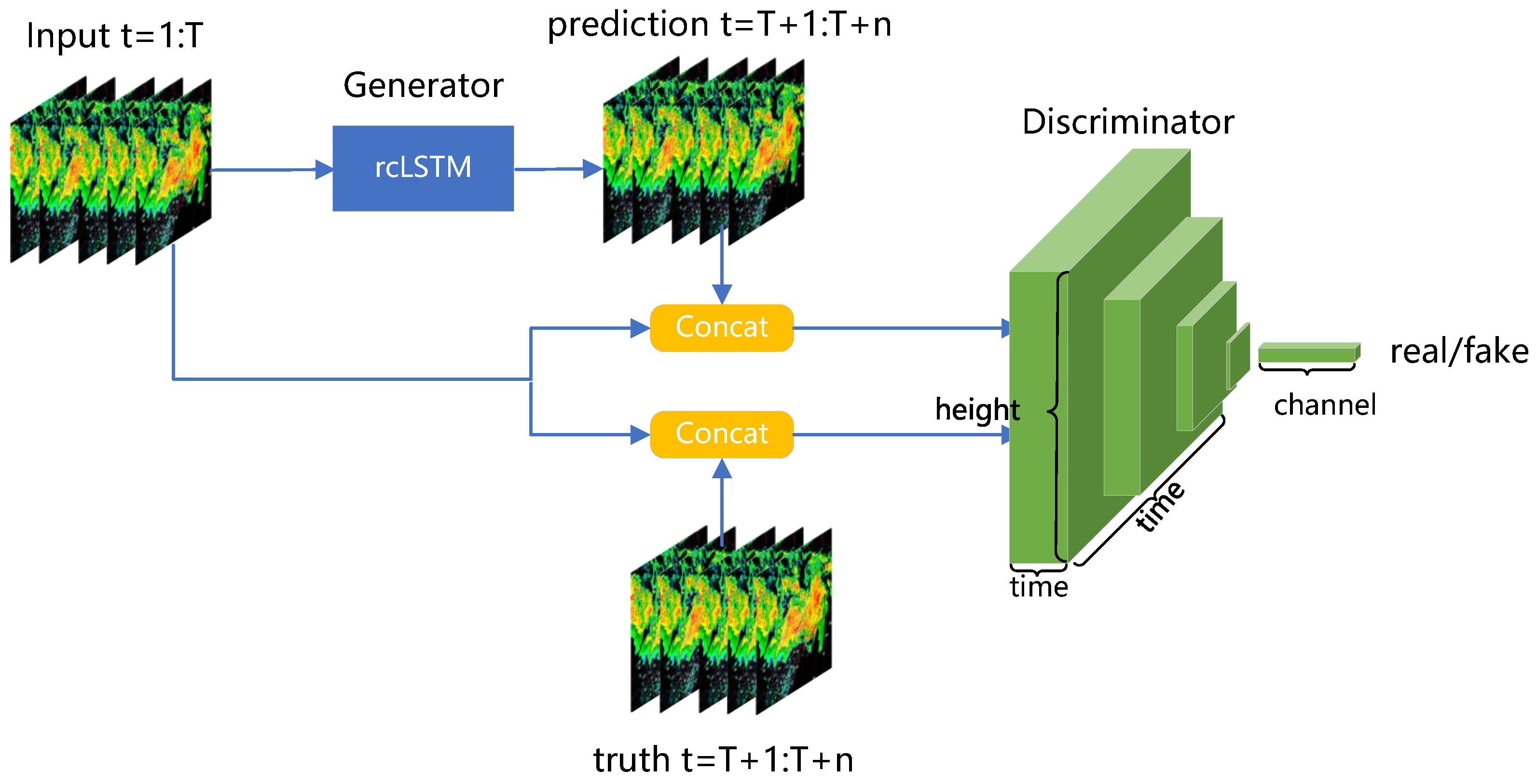
We introduced the generative adversarial networks [42] in the field of unsupervised learning in recent years to solve the fuzzy problem. We replaced the original generator with rcLSTM and replaced the noise with historical radar observations as input. In order to speed up the convergence of the model, we used Layer Normalization between the convolutional layers. The generator is used to generate the echo sequence of the next t times and then concatenated with the real value of the previous t times as a whole. The discriminator is used to distinguish whether it is a complete real value or a generated value. The loss function is Binary Cross Entropy, and the optimization process can be expressed as follows:
max D V ( D , G ) = E x p data ( x ) [ log ( D ( x 1 : T + n ) ) ] + E x p data ( x ) [ log ( 1 D ( [ x 1 : T , G ( x 1 : T ) ) ] ) ] min G V ( D , G ) = E x p data ( x ) [ log ( 1 D ( [ x 1 : T , G ( x 1 : T ) ) ] ) ]
The extrapolated echo sequence became clearer by iteratively alternating training generator and discriminator. During the test phase, only the generator needs to be kept. The structure of the whole model is shown in the Figure 2. The optimization process is shown in Algorithm 1. In the early stage of training, the generator was weak, and the generated samples were significantly different from the real data. Since the discriminator can easily identify false samples, log 1 D x 1 : T ( i ) G x 1 : T ( i ) saturates quickly and cannot provide enough gradients. So, in practice, the generator can be trained to maximize log D x 1 : T ( i ) G x 1 : T ( i ) .
Algorithm 1: Minibatch stochastic gradient descent training of GAN-rcLSTM. The hyperparameter k for the number of steps applied to the discriminator is set to 4.
  • for number of training iterations do
  •    for k steps do
  •      • Sample minibatch of m samples with length T + n { x 1 : T + n ( 1 ) , , x 1 : T + n ( m ) } from ground truth generating distribution p data ( x ) .
  •      • Update the discriminator by ascending its stochastic gradient:
  •             θ d 1 m i = 1 m log D x 1 : T + n ( i ) + log 1 D x 1 : T ( i ) G x 1 : T ( i )
  •    end for
  •    • Sample minibatch of m samples with length T + n { x 1 : T + n ( 1 ) , , x 1 : T + n ( m ) } from ground truth generating distribution p data ( x ) .
  •    • Update the generator by descending its stochastic gradient:
  •           θ g 1 m i = 1 m log 1 D x 1 : T ( i ) G x 1 : T ( i )
  • end for
  • Any standard gradient-based learning rule can be used for gradient-based updates.

2.3. Data

We used RadarJS as the data set, which is provided by Jiangsu Meteorological Observatory of China and covers the years 2017 to 2018. The detailed features of the radar are shown in Table 2. The average elevation in Jiangsu is less than 50 m, and the plain area accounts for 86.89%, which greatly reduces the impact of ground clutter. The radar echo map is made up of 7 Doppler climate radar stations, which are scanned every 6 min, covering an area of about 311 km × 352 km (117.2° E–121.0° E, 31.9° N–34.7° N). After the conversion of the Cartesian coordinate system, the composite reflectivity was obtained, that is, the maximum value of the vertical projection of different elevation angles on the ground. The original radar resolution was 523 × 523 . Considering the limitations of existing computing power, we used average pooling to downsample all data. After processing, the resolution of the radar echo map was 100 × 100 . In order to further improve the data quality, we only kept the summer data (May–August) and filtered out some anomalous fragments such as hardware failure, biological interference, and electromagnetic interference. Finally, the 8 month radar data were divided into 71 consecutive, unequal length data files. Moreover, 65 files were randomly selected as the training set and the remaining 6 as the test set. We extracted 10,080 sequences from the training set and 1580 sequences from the test set. Considering the current computing power and the needs of meteorological operations application, the predicted length of our use case is 10 frames (1 h) and 20 frames (3 h). All use cases in the test set were only used for evaluation and display on the screen, and they were not fed into the model.

3. Results

3.1. Implementation

All experiments are implemented on Pytorch, and we use Adam [43] as the optimizer with L2 loss. In order to make the results comparable, all models have comparable roughly equal parameters numbers. The model consists of 4 layers of LSTM, and each layer of hidden states is 64. The batch size is set to 8, and the starting learning rate is 10 3 . During the whole training process, the random seed is fixed to 0. All models will be trained for 20 epochs on a computer with a single NVIDIA GTX 1080ti GPU. We use Critical success index (CSI), false alarm rate (FAR), and probability of detection (POD) as metrics to evaluate model prediction accuracy. The three skill scores are defined as:
CSI = hits hits + misses + falsealarms FAR = falsealarms hits + falsealarms POD = hits hits + misses
where hits (prediction > threshold, truth > threshold), misses (prediction < threshold, truth > threshold), and false alarms (prediction > threshold, truth < threshold) will be calculated pixel by pixel. In our experiment, the thresholds are set to 10, 20, and 30 dBZ. Higher CSI and POD denote a better prediction result.
To show the predictive ambiguity problem, we use three different methods as quantitative metrics. The first is the pixel-based method called the Sum of Modulus of gray Difference (SMD) [44], the second is the Tenengrad [45] method based on the gradient magnitude, and the third is the Laplacian operator method [46,47] based on the second derivative. I ( m , n ) represents the radar echo intensity function of size N × M .
SMD calculates the sharpness of the image by differentiating adjacent pixels in the horizontal and vertical directions and then using the accumulated value of their modulus values. The calculation process is as follows:
S M D ( I ) = m M n N { | f ( m + 1 , n ) f ( m , n ) | + | f ( m , n + 1 ) f ( m , n ) | }
The Tenengrad method uses the Sobel operator to extract the edge. The calculation process of the Sobel operator and the gradient magnitude is shown as follows:
S x = 1 0 1 2 0 2 1 0 1 S y = 1 2 1 0 0 0 1 2 1
S ( m , n ) = G x ( m , n ) 2 + G y ( m , n ) 2
where the G x and G y are, respectively, the convolution of the input image I ( m , n ) with S x and S y . The Tenengrad ambiguity of the entire image is the sum of the squares of the gradient magnitudes:
T E N ( I ) = m M n N [ S ( m , n ) ] 2
The Laplacian method extracts the high-frequency components of the image through the Laplacian operator, and then uses the sum or variance as the sharpness of the image:
L = 1 6 0 1 0 1 4 1 0 1 0
L A P ( I ) = m M n N | L ( m , n ) | L A P V A R ( I ) = m M n N [ | L ( m , n ) | L ¯ ] 2 L ¯ = 1 N M m M n N | L ( m , n ) |

3.2. Discussion

For LSTM-like networks, depth is the hyperparameter that affects the results most significantly, and Table 3 shows the MSE scores of models with different depths. The results in the table show that when the number of layers is lower than five, with the increase in depth, the fitting ability of all models is gradually enhanced, and the prediction error is gradually reduced. However, when the number of layers exceeds five, the errors of other models no longer decrease and even increase, while the error of rcLSTM can still continue to decrease. Although the seven-layer rcLSTM can achieve better prediction results, in order to make the number of parameters of all models comparable and the training cost of the models acceptable, we fix the depth of all models to four.
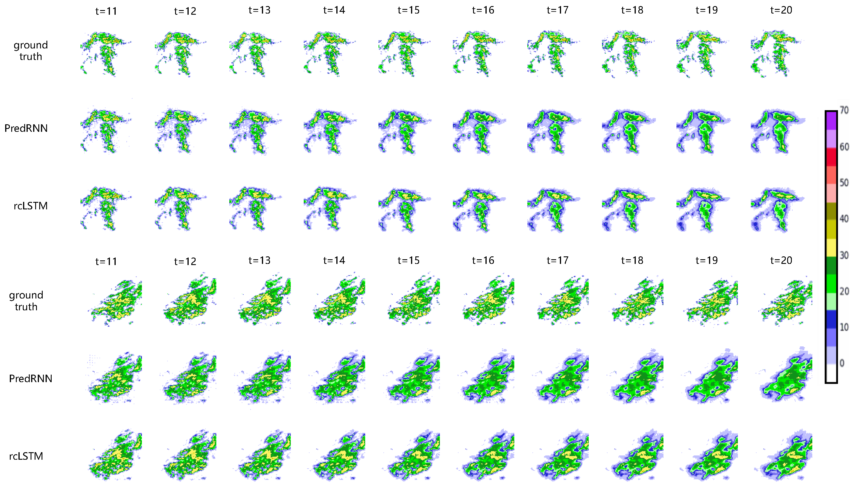
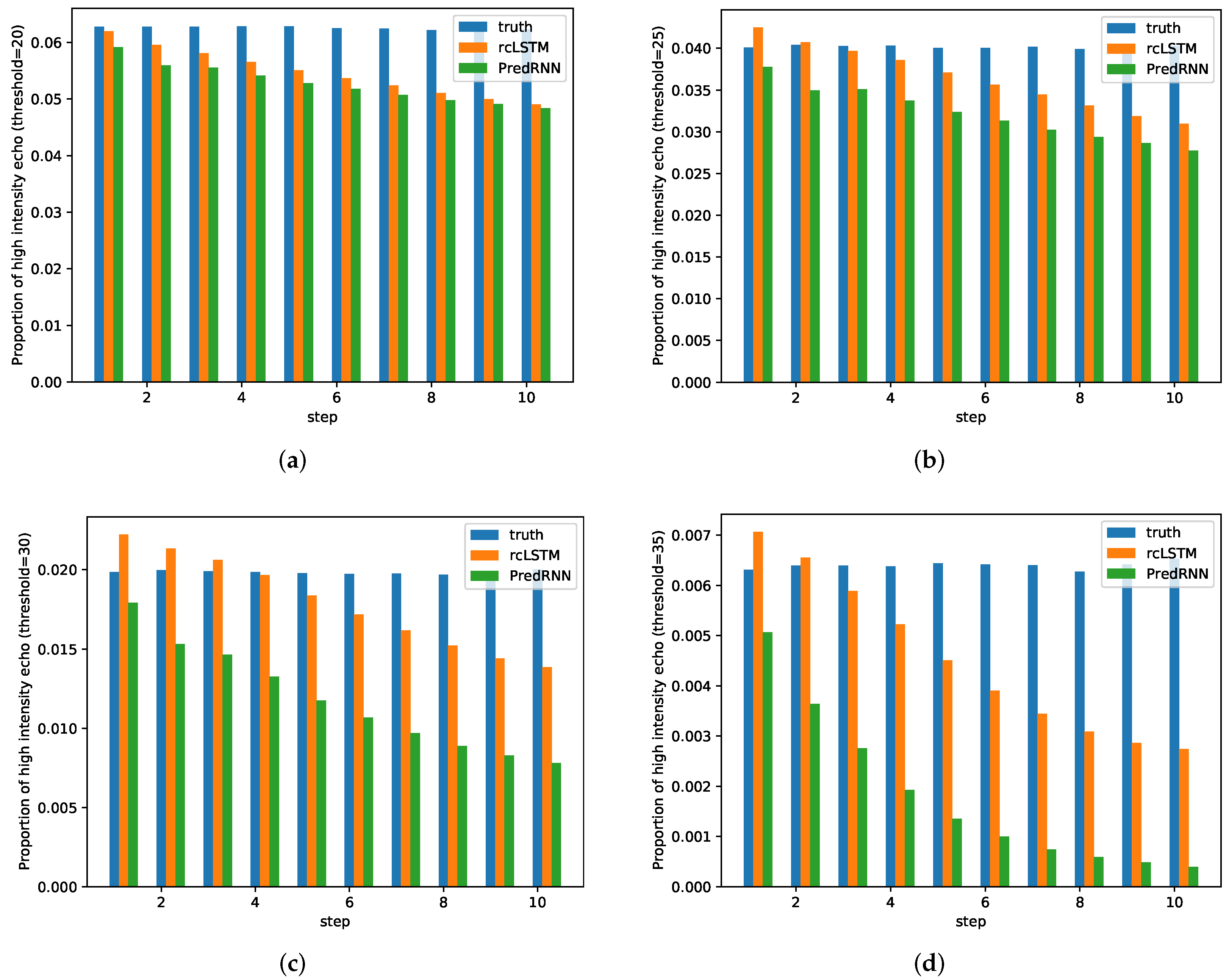
Figure 3 shows two prediction examples of PredRNN and its improved model rcLSTM. In the prediction sequence of PredRNN, the echo with yellow color code (intensity greater than 30 dbz) disappears after five times, while rclstm can stably maintain the echo intensity. Figure 4 shows the proportion of the high-intensity echo. We can find that the echo intensity distribution of PredRNN shows a rapid downward trend, while the distribution of rcLSTM is closer to the real value, which is more obvious at a high threshold. The experimental results show that rcLSTM has stronger retention ability for high-intensity echo.
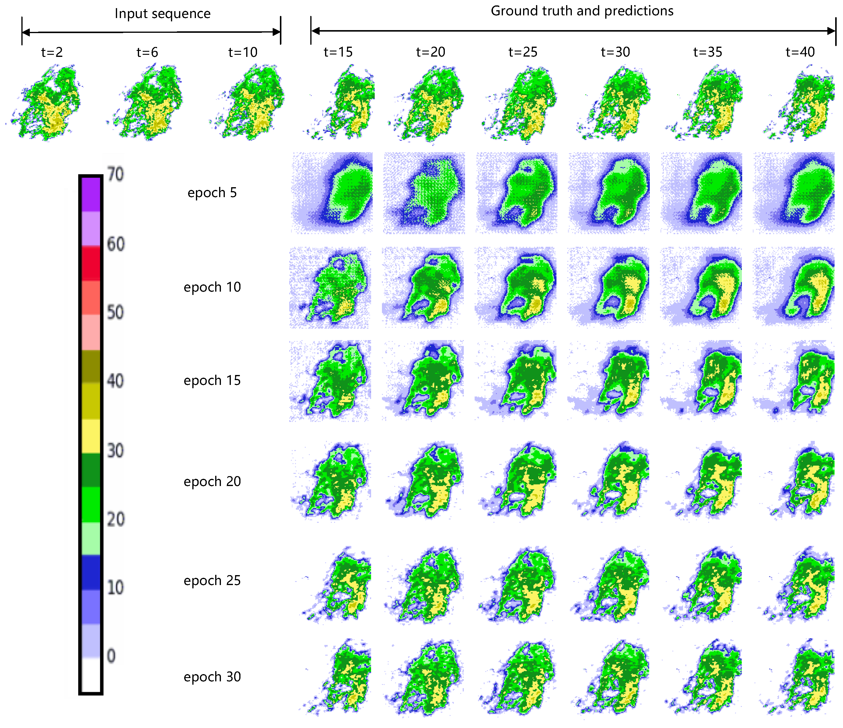
The sequence length was extended to 30 in order to compare the performance of each model in longer forecast period. Figure 5 shows the process of GAN-rcLSTM making the extrapolation results gradually clear. The first row is the sequence of real observations. Lines 2 to 7 are the extrapolation results. In the initial stage, the prediction effect of GAN-rcLSTM is very blurred and distorted. In the 10th epoch, high-intensity echoes greater than 30 dBZ in the southeast direction could already be predicted. In the 15th to the 20th epochs, the edge of the echo is sharper, and the details are closer to the real value, but there is still an error in the generated echo motion trajectory, and the overall orientation is biased to the west. The sequences generated in epoch 25 to 30 are sharper, while the low-intensity noise echoes with an intensity less than 5 dbz at the edges are significantly reduced.
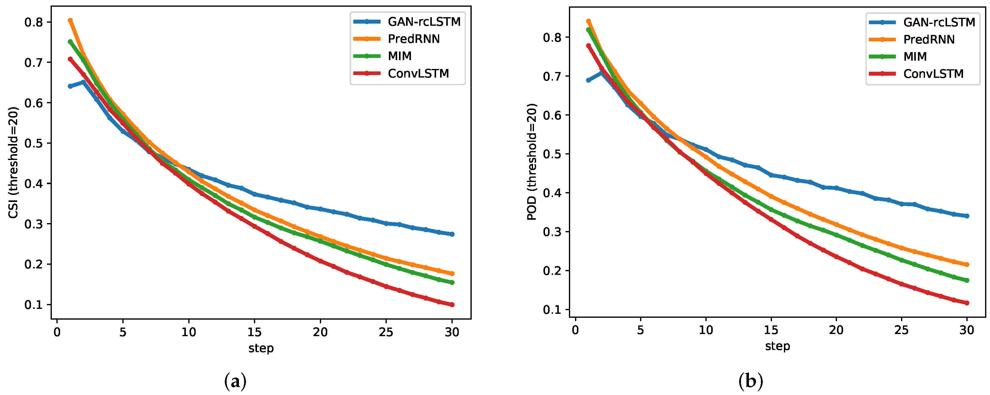
Figure 6 shows the frame-wise accuracy scores of all models on the test set. We can find that the score drop of the GAN-rcLSTM is more gradual compared to other models. After 10 steps, our model outperformed the other models in both CSI and POD scores. We visualize two examples in Figure 7. GAN-rcLSTM maintains steady sharpness for three hours of forecast, while all other models start to blur after half an hour. Table 4 shows the average accuracy scores of all models. We can find that GAN-rcLSTM does not achieve the best MSE score because the loss function during training is Binary Cross Entropy (BCE). However, it is more meaningful that it achieves the highest CSI and POD metrics within the acceptable FAR range.
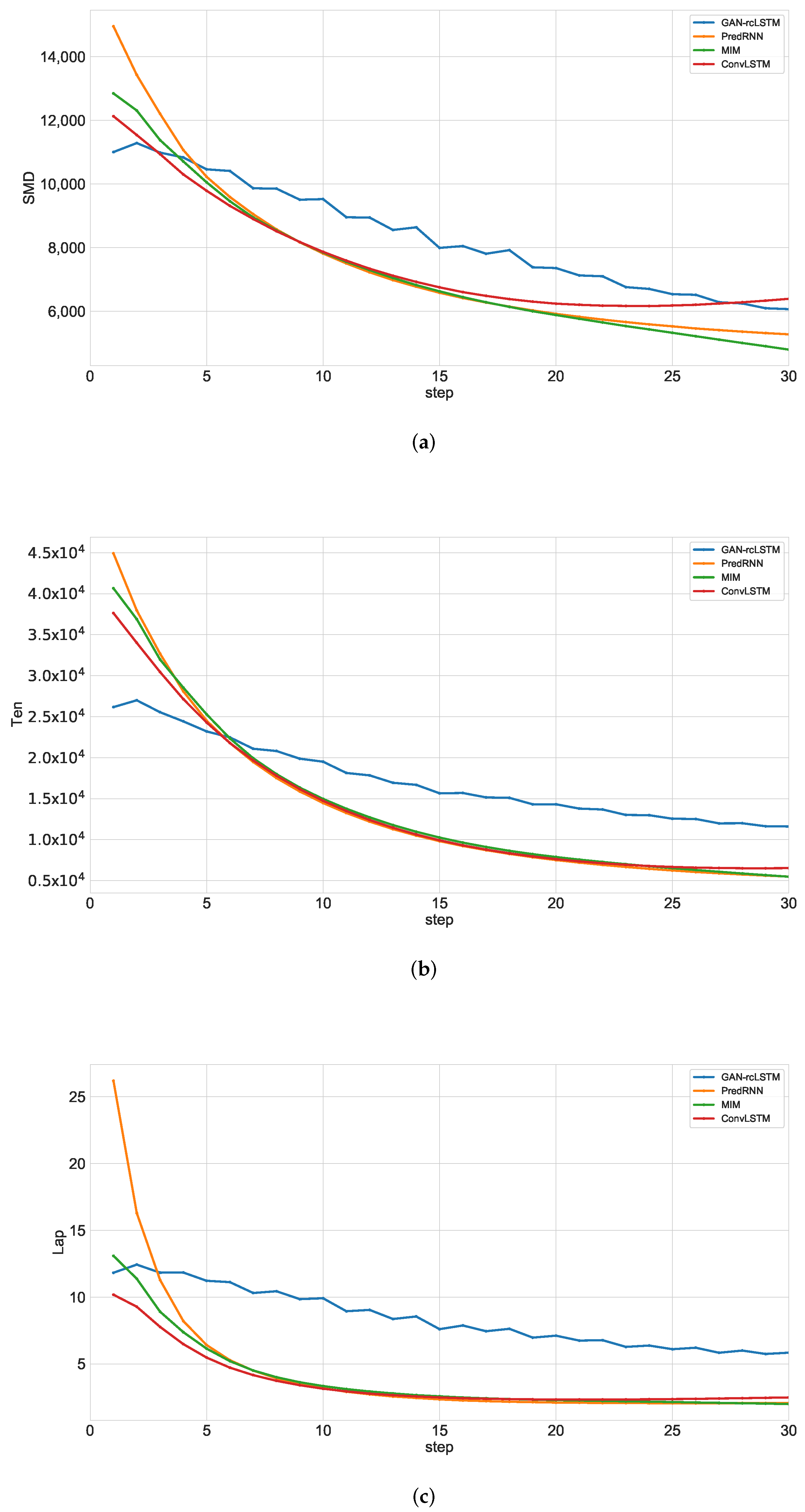
Figure 8 and Table 5 show the change in sharpness of the prediction process for different models. The scores of LSTM-like models drop rapidly after 5 frames (half an hour), while GAN-rcLSTM can maintain a relatively stable sharpness. Because LSTM calculates the mean square error time by time independently and then calculates the average value when calculating the loss, the later frames will therefore be more and more conservative in order to avoid gradient punishment, while GAN-rcLSTM takes the prediction sequence as a whole and simulates the real radar echo indexing through the constraints of the discriminator. We think that GAN-rcLSTM can provide better forecasts in short-term forecasting tasks.
After training, GAN-rcLSTM only keeps the generator and no longer needs the discriminator. So, forecast speed is perfectly acceptable in an operational setting. Table 6 shows the time consumed for different models to make predictions. The GPU used in the experiment is an Nvidia GTX 1080ti and the CPU is AMD Ryzen 7 2700X. We can find that the speed of GAN-rcLSTM is about the same as other models. Furthermore, even without GPU acceleration, the prediction time of GAN-rcLSTM is much lower than the period of radar update (6 min).

4. Conclusions

We investigate the problem of echo decay and blurring, which are the main drawbacks of LSTM-based radar extrapolation methods. This paper proposes a new recurrent neural network (rcLSTM) to overcome the degradation phenomenon of deep LSTM networks. We enhance the gradient transfer between multi-layer LSTMs by adding residual modules. Furthermore, we use rcLSTM as a generator and extend GAN-rcLSTM to solve the blurring problem in long sequence prediction. GAN-rcLSTM achieves the highest prediction accuracy score and the lowest ambiguity on the Jiangsu radar echo dataset.In order to further improve the prediction accuracy of radar echo generation and cancellation changes, we will also try to use an attention mechanism and an encoding–decoding structure to integrate multi-source observation data in the future.

Author Contributions

Conceptualization, T.W.; methodology, T.W.; software, T.W.; validation, T.W.; formal analysis, T.W.; investigation, T.W. and Z.H. and L.G.; resources, H.G.; data curation, X.Z. and D.X.; writing—original draft preparation, T.W.; writing—review and editing, H.G.; visualization, T.W.; supervision, H.G.; project administration, H.G.; funding acquisition, H.G. All authors have read and agreed to the published version of the manuscript.

Funding

This research was funded by NanJing Joint Center of Atmospheric Research under Grant NJCAR2018MS05, National Key Research Development Plan under Grant 2017YFC1502104 and the Beijige foundationof NJIAS under Grant BJG202103.

Institutional Review Board Statement

Not applicable.

Informed Consent Statement

Not applicable.

Data Availability Statement

The data presented in this study are available on request from the corresponding author. The data are not publicly available due to the confidentiality policy of Jiangsu Meteorological Observatory.

Conflicts of Interest

The authors declare no conflict of interest.

References

  1. Johnson, J.; MacKeen, P.; Witt, A.; Mitchell, E.; Stumpf, G.; Eilts, M.; Thomas, K. The Storm Cell Identification and Tracking Algorithm: An Enhanced WSR-88D Algorithm. Weather Forecast. 1998, 13, 263–276. [Google Scholar] [CrossRef] [Green Version]
  2. Dixon, M.; Wiener, G. TITAN: Thunderstorm Identification, Tracking, Analysis, and Nowcasting—A Radar-based Methodology. J. Atmos. Ocean. Technol. 1993, 10, 785. [Google Scholar] [CrossRef]
  3. Li, L.; Schmid, W.; Joss, J. Nowcasting of Motion and Growth of Precipitation with Radar over a Complex Orography. J. Appl. Meteorol. 1995, 34, 1286–1300. [Google Scholar] [CrossRef] [Green Version]
  4. Rinehart, R.E.; Garvey, E.T. Three-dimensional storm motion detection by conventional weather radar. Nature 1978, 273, 287–289. [Google Scholar] [CrossRef]
  5. Farneback, G. Very high accuracy velocity estimation using orientation tensors, parametric motion, and simultaneous segmentation of the motion field. In Proceedings of the IEEE International Conference on Computer Vision, Vancouver, BC, Canada, 7–14 July 2001; Volume 1, pp. 171–177. [Google Scholar] [CrossRef] [Green Version]
  6. Sakaino, H. Spatio-Temporal Image Pattern Prediction Method Based on a Physical Model With Time-Varying Optical Flow. IEEE Trans. Geoence Remote Sens. 2013, 51, 3023–3036. [Google Scholar] [CrossRef]
  7. Germann, U.; Zawadzki, I. Scale-Dependence of the Predictability of Precipitation from Continental Radar Images. Part I: Description of the Methodology. Mon. Weather Rev. 2001, 130, 2859–2873. [Google Scholar] [CrossRef]
  8. Lucas, B.D.; Kanade, T. An iterative image registration technique with an application to stereo vision. In Proceedings of the 7th International Joint Conference on Artificial Intelligence, Vancouver, BC, Canada, 24–28 August 1981; Volume 2, pp. 674–679. [Google Scholar]
  9. Weinzaepfel, P.; Revaud, J.; Harchaoui, Z.; Schmid, C. DeepFlow: Large Displacement Optical Flow with Deep Matching. In Proceedings of the IEEE International Conference on Computer Vision, Sydney, Australia, 1–8 December 2013; pp. 1385–1392. [Google Scholar] [CrossRef] [Green Version]
  10. Wulff, J.; Black, M.J. Efficient sparse-to-dense optical flow estimation using a learned basis and layers. In Proceedings of the IEEE Conference on Computer Vision and Pattern Recognition, Boston, MA, USA, 7–12 June 2015; pp. 120–130. [Google Scholar] [CrossRef]
  11. Elsayed, N.; Maida, A.S.; Bayoumi, M. Reduced-Gate Convolutional LSTM Architecture for Next-Frame Video Prediction Using Predictive Coding. In Proceedings of the International Joint Conference on Neural Networks, Budapest, Hungary, 14–19 July 2019; pp. 1–9. [Google Scholar] [CrossRef]
  12. Kalchbrenner, N.; Oord, A.; Simonyan, K.; Danihelka, I.; Vinyals, O.; Graves, A.; Kavukcuoglu, K. Video Pixel Networks. In Proceedings of the International Conference on Machine Learning, Sydney, Australia, 6–11 August 2017; Volume 70, pp. 1771–1779. [Google Scholar]
  13. Lotter, W.; Kreiman, G.; Cox, D. Deep predictive coding networks for video prediction and unsupervised learning. In Proceedings of the International Conference on Learning Representations, Toulon, France, 24–26 April 2017. [Google Scholar]
  14. Oliu, M.; Selva, J.; Escalera, S. Folded Recurrent Neural Networks for Future Video Prediction. In Proceedings of the European Conference on Computer Vision, Munich, Germany, 8–14 September 2018; pp. 716–731. [Google Scholar] [CrossRef] [Green Version]
  15. Denton, E.; Birodkar, V. Unsupervised learning of disentangled representations from video. In Proceedings of the Conference and Workshop on Neural Information Processing Systems, Long Beach, CA, USA, 4–9 December 2017; Curran Associates Inc.: Red Hook, NY, USA, 2017; Volume 30, pp. 4417–4426. [Google Scholar]
  16. Ham, Y.; Kim, J.; Luo, J. Deep learning for multi-year ENSO forecasts. Nature 2019, 573, 568–572. [Google Scholar] [CrossRef]
  17. Oh, J.; Guo, X.; Lee, H.; Lewis, R.; Singh, S. Action-conditional video prediction using deep networks in Atari games. In Proceedings of the Conference and Workshop on Neural Information Processing Systems, Montreal, QC, USA, 7–12 December 2015; MIT Press: Cambridge, MA, USA, 2015; Volume 28, pp. 2863–2871. [Google Scholar]
  18. Villegas, R.; Yang, J.; Zou, Y.; Sohn, S.; Lin, X.; Lee, H. Learning to generate long-term future via hierarchical prediction. In Proceedings of the International Conference on Machine Learning, Sydney, Australia, 6–11 August 2017; Volume 70, pp. 3560–3569. [Google Scholar]
  19. He, W.; Xiong, T.; Wang, H.; He, J.; Ren, X.; Yan, Y.; Tan, L. Radar Echo Spatiotemporal Sequence Prediction Using an Improved ConvGRU Deep Learning Model. Atmosphere 2022, 13, 88. [Google Scholar] [CrossRef]
  20. Chen, S.; Zhang, S.; Geng, H.; Chen, Y.; Zhang, C.; Min, J. Strong Spatiotemporal Radar Echo Nowcasting Combining 3DCNN and Bi-Directional Convolutional LSTM. Atmosphere 2020, 11, 569. [Google Scholar] [CrossRef]
  21. Geng, H.; Geng, L. MCCS-LSTM: Extracting Full-Image Contextual Information and Multi-Scale Spatiotemporal Feature for Radar Echo Extrapolation. Atmosphere 2022, 13, 192. [Google Scholar] [CrossRef]
  22. Elman, J.L. Finding Structure in Time. Cogn. Sci. 1990, 14, 179–211. [Google Scholar] [CrossRef]
  23. Hochreiter, S.; Schmidhuber, J. Long Short-Term Memory. Neural Comput. 1997, 9, 1735–1780. [Google Scholar] [CrossRef] [PubMed]
  24. Cho, K.; Merrienboer, B.; Bahdanau, D.; Bougares, F.; Schwenk, H.; Bengio, Y. Learning Phrase Representations using RNN Encoder-Decoder for Statistical Machine Translation. In Proceedings of the Conference on Empirical Methods in Natural Language Processing, Doha, Qatar, 25–29 October 2014; pp. 1724–1734. [Google Scholar] [CrossRef]
  25. Srivastava, N.; Mansimov, E.; Salakhutdinov, R. Unsupervised learning of video representations using LSTMs. In Proceedings of the International Conference on Machine Learning, Lille, France, 6–11 July 2015; Volume 37, pp. 843–852. [Google Scholar]
  26. Shi, X.; Chen, Z.; Wang, H.; Yeung, D.; Wong, W.; Woo, W. Convolutional LSTM Network: A machine learning approach for precipitation nowcasting. In Proceedings of the Conference and Workshop on Neural Information Processing Systems, Montreal, QC, USA, 7–12 December 2015; MIT Press: Cambridge, MA, USA, 2015; Volume 1, pp. 802–810. [Google Scholar]
  27. Brabandere, B.; Jia, X.; Tuytelaars, T.; Van Gool, L. Dynamic Filter Networks. In Proceedings of the Conference and Workshop on Neural Information Processing Systems, Barcelona, Spain, 5–10 December 2016; Volume 29, pp. 667–675. [Google Scholar]
  28. Shi, X.; Gao, Z.; Lausen, L.; Wang, H.; Yeung, D.; Wong, W.; Woo, W. Deep learning for precipitation nowcasting: A benchmark and a new model. In Proceedings of the Conference and Workshop on Neural Information Processing Systems, Long Beach, CA, USA, 4–9 December 2017; Curran Associates Inc.: Red Hook, NY, USA, 2017; Volume 30, pp. 5622–5632. [Google Scholar]
  29. Wang, Y.; Long, M.; Wang, J.; Gao, Z.; Yu, P.S. PredRNN: Recurrent Neural Networks for Predictive Learning using Spatiotemporal LSTMs. In Proceedings of the Conference and Workshop on Neural Information Processing Systems, Long Beach, CA, USA, 4–9 December 2017; Volume 30, pp. 879–888. [Google Scholar]
  30. Wang, Y.; Gao, Z.; Long, M.; Wang, H.; Yu, P.S. PredRNN++: Towards A Resolution of the Deep-in-Time Dilemma in Spatiotemporal Predictive Learning. In Proceedings of the International Conference on Machine Learning, Stockholm, Sweden, 10–15 July 2018; Volume 80, pp. 5123–5132. [Google Scholar]
  31. Srivastava, R.K.; Greff, K.; Schmidhuber, J. Training very deep networks. In Proceedings of the Conference and Workshop on Neural Information Processing Systems, Montreal, QC, USA, 7–12 December 2015; Volume 28, pp. 2377–2385. [Google Scholar]
  32. Wang, Y.; Zhang, J.; Zhu, H.; Long, M.; Wang, J.; Yu, P.S. Memory in Memory: A Predictive Neural Network for Learning Higher-Order Non-Stationarity From Spatiotemporal Dynamics. In Proceedings of the IEEE Conference on Computer Vision and Pattern Recognition, Long Beach, CA, USA, 16–20 June 2019; pp. 9154–9162. [Google Scholar]
  33. Wang, Y.; Jiang, L.; Yang, M.; Li, L.; Long, M.; Li, F. Eidetic 3D LSTM: A Model for Video Prediction and Beyond. In Proceedings of the International Conference on Learning Representations, New Orleans, LA, USA, 6–9 May 2019. [Google Scholar]
  34. Ravuri, S.; Lenc, K.; Willson, M.; Kangin, D.; Lam, R.; Mirowski, P.; Fitzsimons, M.; Athanassiadou, M.; Kashem, S.; Madge, S.; et al. Skilful precipitation nowcasting using deep generative models of radar. Nature 2021, 597, 672–677. [Google Scholar] [CrossRef] [PubMed]
  35. Simonyan, K.; Zisserman, A. Very Deep Convolutional Networks for Large-Scale Image Recognition. arXiv 2014, arXiv:1409.1556. [Google Scholar]
  36. Krizhevsky, A.; Sutskever, I.; Hinton, G.E. ImageNet classification with deep convolutional neural networks. Commun. ACM 2017, 60, 84–90. [Google Scholar] [CrossRef]
  37. Cun, L.; Boser, Y.; Denker, B.; Henderson, D.; Howard, R.; Hubbard, W.; Jackel, L. Backpropagation Applied to Handwritten zip code Recognition. Neural Comput. 1989, 1, 541–551. [Google Scholar]
  38. Szegedy, C.; Wei, L.; Yangqing, J.; Sermanet, P.; Reed, S.; Anguelov, D.; Erhan, D.; Vanhoucke, V.; Rabinovich, A. Going deeper with convolutions. In Proceedings of the IEEE Conference on Computer Vision and Pattern Recognition, Boston, MA, USA, 7–12 June 2015; pp. 1–9. [Google Scholar] [CrossRef] [Green Version]
  39. He, K.; Zhang, X.; Ren, S.; Sun, J. Deep Residual Learning for Image Recognition. In Proceedings of the IEEE Conference on Computer Vision and Pattern Recognition, Las Vegas, NV, USA, 27–30 June 2016; pp. 770–778. [Google Scholar]
  40. He, K.; Sun, J. Convolutional neural networks at constrained time cost. In Proceedings of the Conference on Computer Vision and Pattern Recognition, Boston, MA, USA, 7–12 June 2015; pp. 5353–5360. [Google Scholar] [CrossRef] [Green Version]
  41. Srivastava, R.K.; Greff, K.; Schmidhuber, J. Highway Networks. arXiv 2015, arXiv:1505.00387. [Google Scholar]
  42. Goodfellow, I.J.; Pouget-Abadie, J.; Mirza, M.; Xu, B.; Warde-Farley, D.; Ozair, S.; Courville, A.C.; Bengio, Y. Generative Adversarial Nets. In Proceedings of the Conference and Workshop on Neural Information Processing Systems, Montréal, QC, Canada, 8–13 December 2014; Volume 27, pp. 2672–2680. [Google Scholar]
  43. Kingma, D.; Ba, J. Adam: A Method for Stochastic Optimization. arXiv 2015, arXiv:1412.6980. [Google Scholar]
  44. Jarvis, R. Focus optimisation criteria for computer image processing. Microscope 1976, 24, 163–180. [Google Scholar]
  45. Krotkov, E. Focusing. Int. J. Comput. Vis. 1987, 1, 223–227. [Google Scholar] [CrossRef]
  46. Pech-Pacheco, J.; Cristobal, G.; Chamorro-Martinez, J.; Fernandez-Valdivia, J. Diatom autofocusing in brightfield microscopy: A comparative study. In Proceedings of the 15th International Conference on Pattern Recognition., Barcelona, Spain, 3–7 September 2000; Volume 3, pp. 314–317. [Google Scholar] [CrossRef]
  47. Nayar, S.; Nakagawa, Y. Shape from focus system. IEEE Trans. Pattern Anal. Mach. Intell. 1994, 16, 824–831. [Google Scholar] [CrossRef] [Green Version]
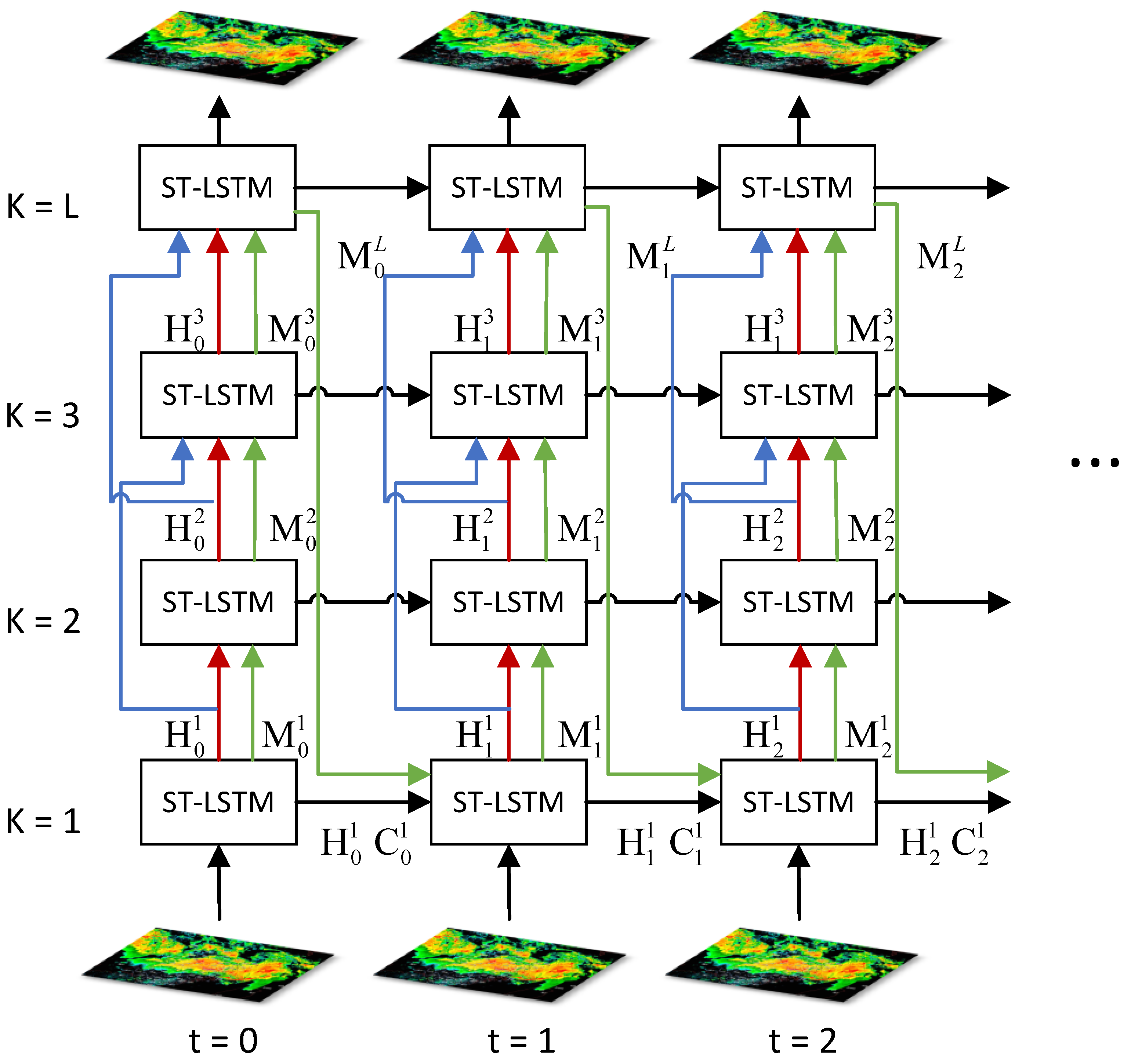
Figure 1. The structure of the rc-LSTM model. The green arrow shows the transition paths of state M, the red arrow shows the transition paths of the hidden state H. The subscript represents the time and the superscript represents the layer. rcLSTM adopts a series structure, and the output of the bottom layer is used as the input of the high layer. In particular, the output of the highest layer represents the predicted value of the next moment. For the first layer, in the feature extraction stage, the input of each moment is the real observation value of the radar echo, and in the prediction stage, the predicted radar echo of the previous moment is used as the input of the next moment.
Atmosphere 13 00684 g001
Figure 2. The structure of the GAN-rcLSTM model.
Atmosphere 13 00684 g002
Figure 3. Examples of the next-hour predictions at 5:10 on 2 May 2017 and 15:16 on 22 May 2017 in Jiangsu, China. From top to bottom are the ground truth, PredRNN prediction result, and rcLSTM prediction result. The radar echo intensity is represented by different colors, in which blue represents 0–15 dbz, green represents 15–30 dbz, and yellow represents 30–40 dbz.
Atmosphere 13 00684 g003
Figure 4. The height of the bar is between 0 and 1, indicating the proportion of echoes in the area that are above the threshold. Among them, the blue one represents the true value, the yellow one is the prediction result of rcLSTM, and the green one represents the PredRNN. In (ad), the thresholds are set to 20, 25, 30, and 35, respectively.
Atmosphere 13 00684 g004
Figure 5. Prediction results of GAN-rcLSTM at different training stages.
Atmosphere 13 00684 g005
Figure 6. Comparison of predictions from different models for the next 30 frames, with a 6-min interval between each frame. (a) is the Critical success index (CSI), (b) is the probability of detection (POD), (c) is the false alarm rate (FAR), and (d) is the mean square error (MSE). High CSI and POD curves indicate more accurate hits, low MSE and FAR curves indicate lower errors and false positives.
Atmosphere 13 00684 g006aAtmosphere 13 00684 g006b
Figure 7. Examples of the next three hour predictions at 15:16 on 22 May 2017 and 9:54 on 28 July 2017 in Jiangsu, China. Lines 2–4 are the prediction result of ConvLSTM, PredRNN, MIM, and GAN-rcLSTM for each example. The interval between the displayed predicted images and the input images is 30 min and 24 min, respectively. The radar echo intensity is represented by different colors, in which blue represents 0–15 dbz, green represents 15–30 dbz, and yellow represents 30–40 dbz.
Atmosphere 13 00684 g007
Figure 8. Comparison of predictions from different models for the next 30 frames, with a 6-min interval between each frame. (a) is the Sum of Modulus of gray Difference, (b) is the Tenengrad, and (c) is the Laplacian variance. A lower curve indicates a clearer extrapolation result.
Atmosphere 13 00684 g008
Table 1. Types of weather forecasts.
Forecast TypesPeriod Validity
nowcasting0–2 h
short-term forecasting0–12 h
short-range forecasting1–3 days
medium-range forecasting4–10 days
long-range forecasting>30 days
Table 2. Radar parameter details.
Radar ParametersValue
BandS
Wavelength10 cm
Frequency2.86 GHZ
Pulse recurrence frequency322–1014 Hz
Pulse width1.57  μ s
Peak power650 KW
Antenna gain44 dB
Antenna aperture8.5 m
Beam width0.95°
Operation modeSTSR
Volume scan modePPI
Sagittal resolution250 m
Table 3. MSE scores for the 10-frames-lead forecast for the models with different depths.
DepthConvLSTMPredRNNMIMrcLSTM
121.32---
220.5818.1818.6118.16
318.2917.6616.9817.32
417.0416.3315.9515.76
517.1216.5115.4915.35
617.0317.2816.7315.28
719.2817.1316.9815.16
Table 4. Quantitative accuracy metrics of prediction results for different methods at a lead of 30 frames.
ModelMSECSIPODFAR
ConvLSTM34.6290.3230.3600.268
PredRNN33.5080.3730.4240.298
MIM31.3660.3560.3950.235
GAN-rcLSTM32.6620.4020.4720.259
Table 5. Quantitative sharpness metrics of prediction results for different methods at a lead of 30 frames.
ModelSMDTenengradLaplacian
ConvLSTM75821,370,6203.582
PredRNN75341,394,0624.441
MIM73001,408,2763.824
GAN-rcLSTM83561,719,0498.406
Table 6. Time consumed for different models to make predictions. Each pair of numbers represents the time spent using GPU acceleration and using only the CPU. The statistical results are from the average time-consuming of 20 runs, in seconds.
ModelTime Required to
Predict 10 Frames (GPU/CPU)
Time Required to
Predict 20 Frames (GPU/CPU)
Time Required to
Predict 30 Frames (GPU/CPU)
ConvLSTM0.7 s/48.5 s1.0 s/75.4 s2.3 s/126.8 s
PredRNN0.9 s/51.2 s1.5 s/78.3 s2.2 s/131.9 s
MIM1.8 s/57.8 s2.9 s/94.8 s3.9 s/143.0 s
GAN-rcLSTM0.9 s/51.4 s1.5 s/82.0 s2.3 s/134.2 s
Publisher’s Note: MDPI stays neutral with regard to jurisdictional claims in published maps and institutional affiliations.