Abstract
Currently, many researchers have an interest in the investigation of the electric field in the fair-weather electric environment along with its diurnal and seasonal variations across all regions of the world. However, a similar study in the southern part of Western Siberia has not yet been carried out. In this regard, the paper aims to estimate the mean values of the electric field and their variations in this area using the example of Tomsk. The time series of one-minute average potential gradient values as well as other quantities obtained from the geophysical observatory of the Institute of Monitoring of Climatic and Ecological Systems of the Siberian Branch of the Russian Academy of Sciences (IMCES SB RAS, Tomsk, Russia) from 2006 to 2020 is used in this study. The mean annual value of the potential gradient in Tomsk is 282 V/m and usually varies from 161 to 372 V/m. The diurnal variations in potential gradient per year on average are characterized by oscillations of the continental type with a double maximum and minimum. The main minimum of diurnal variations is 7 h and the main maximum is 21 h of local time (00 and 14 UTC, respectively). According to the annual mode, the maximum potential gradient is observed in February, and the minimum is recorded in June.
1. Introduction
Measurements of the characteristics of atmospheric electricity in the surface layer, usually the electric field, provide information on both the local electrical state and the functioning of the entire Global Electric Circuit (GEC). The first measurements of a predominantly experimental nature began more than 150 years ago. Improvements to existing instrumentation contributed to the organization of global systematic observations of electrical quantities such as the potential gradient (∇φ), electrical conductivity of air, ion concentration, current density, and others [1,2,3,4,5,6,7,8]. Today, numerous ground-based measurements provide information about the electrical state of the atmosphere, and different approaches [1,6,9] to data selection and processing have allowed us to draw fundamental conclusions about the influence of fair-weather [1,2,3,4,5,6,7,8,9,10,11,12,13,14,15,16,17,18,19,20,21] and disturbed weather conditions [6,11,12,13,14,15,16,17,18,19,22,23,24,25,26,27,28,29,30,31,32,33,34,35,36,37,38] on the surface atmospheric electricity.
For instance, the studies carried out on the Carnegie geophysical survey vessel in the early twentieth century made it possible to discover one of the global mechanisms affecting the atmospheric electric field. This is the average daily variation in the potential gradient, widely known as the Carnegie curve or unitary variation. It represents the global daily contribution of electrical activity in areas of disturbed weather [1,39] and follows universal time, globally independent of the measurement position [1].
However, the contribution of regional and local factors can significantly affect the diurnal variations in the surface electric field in different regions of the globe. A strong relationship exists between atmospheric aerosols and the electrical characteristics of the atmosphere: aerosols remove light ions from the air, which leads to a decrease in conductivity, and, consequently, the gradient of the electric field potential should increase. Thus, in the polluted urban environment, the surface values of the potential gradient are higher than those in the countryside and are subject to additional fluctuations due to changes in concentration. This effect has been found in many cities around the world [2,6,9,40,41]. The lofting of smoke plumes from wildland fires [42], intense dust storms [43,44], and eruptive clouds from volcanoes [45] spreading in middle and upper atmosphere are all factors contributing to a decrease in the potential gradient.
Meteorological factors have a special place in the study of atmospheric electricity, as they are characterized by greater temporal and spatial variability. Fogs, mist, or haze contributes to an increase in the surface value of the potential gradient [9,10,46]. Short-lived (up to several hours) convective clouds, particularly Cumulonimbus, cause short deviations in the potential gradient with both positive and negative signs [11,36,37]. Mesoscale convective systems and cloud systems associated with atmospheric fronts of temperate and tropical cyclones, which are accompanied by severe thunderstorm activity, cause a severe perturbation of the normal atmospheric electric field over long periods of time and space [30,47,48,49,50].
The diurnal variations in the potential gradient on fair-weather days recorded in different regions of the globe are classified broadly into three types. The potential gradient diurnal variations having a minimum near 04 UTC and a maximum near 19 UTC (as is the case of the Carnegie curve) are considered to be of Type1. The variations having two minima, one at ~02 UTC and the other one at ~10 UTC, and two maxima, one at ~06 UTC and the other at ~19 UTC, are of Type2. The diurnal variations having a broad depression, centered at ~11 UTC, are of Type3 [6,13,51].
As the electrical state of the atmosphere greatly varies due to various regional and local effects, monitoring and analysis of the variability in atmospheric-electrical quantities in different regions of the Earth are necessary for a full understanding of the functioning of the GEC and the relationship of changes in its characteristics with modern climatic changes.
Detailed studies of the atmospheric electrical quantities in Western Siberia covering a significant territory of more than 2 million sq. km have not yet been conducted. The work in this regard aims to estimate the average values of the potential gradient under fair-weather conditions, as well as its daily and seasonal variations in the south of Western Siberia, using Tomsk as an example.
2. Materials and Methods
The study focused on the southern region of Western Siberia, which is located in the central part of Eurasia, far from the oceanic coasts (Figure 1a). The Vasyugan, Ket-Tymkaya, Ishim, and Kulundinskaya plains, as well as the Barabinskaya lowland, make up the majority of the research area. The southeastern part of the territory belongs to the mountainous Salair Ridge and Kuznetsk Alatau, the northern part of the Altai Mountains, and the western part of the Western Sayan. The Vasyugan Swamp, the largest swamp system in the northern hemisphere, is located in the northern part of the study area. This region is characterized by unique physical and geographical conditions and a significant distance from the oceans.
Our research is based on the data of atmospheric-electrical measurements at the geophysical observatory (GO) of the Institute of Monitoring of Climate and Ecological Systems of the Siberian Branch of the Russian Academy of Sciences (hereinafter the IMCES GO). This site is representative of more parts of the study region. The IMCES GO is located 167 m a.s.l. in the eastern part of Tomsk (Russia) at 56.48° N and 85.05° E (Figure 1b). The IMCES GO conducts geophysical, meteorological, and environmental observations, as well as testing and comparing new equipment and technologies. Observations of atmospheric-electrical, actinometric, and meteorological variables, including turbulence, have been made with high temporal resolution (1 min or less) since 2006. A description of the IMCES GO is available on its website [52] (in Russian).

Figure 1.
The region of studies (a) and the location of the IMCES GO (b). The map are shown based on the global digital elevation model ETOPO2 [53].
Figure 1.
The region of studies (a) and the location of the IMCES GO (b). The map are shown based on the global digital elevation model ETOPO2 [53].

Measurements of the potential gradient were conducted by the Field-2 and CS110 field mills with a time averaging of 30 and 1 s, respectively. The Field-2 measures ∇φ in the range of ±5000 V/m with an accuracy of ±5%. The Field-2 was produced and calibrated by the calibrator of electric field strength KNEP-1M (a range of ±5000 V/m, an accuracy of 1.5%) in the Voeikov Main Geophysical Observatory (St. Petersburg, Russia) [54]. More information about this sensor can be seen in [55]. The CS110 was produced and calibrated by the Campbell Scientific, Inc. (Logan, UT, USA) [56]. It measures ∇φ in the range of ±22,300 V/m with an accuracy of ±5%. The CS110 has two ranges of measurement, ±2200 V/m with a resolution 0.32 V/m or ±22,300 V/m with a resolution 3.2 V/m, with automatic switching between them [57].
Both sensors are located next to each other on the ground observation site in accordance with the requirements for installation and measurement. The Field-2 mounts at a height of 1 m on the grounded metal grid (3 by 3 m) and measures ∇φ corrected to ground level [58]. The CS110 is positioned 2 m above ground level on the grounded metal tripod mast and has an additive correction of +8 V/m for reducing to ground level [57]. Taking into account the grounding of the sensors, i.e., correcting their readings to values corresponding to the ground level, and their instrument accuracies, the potential gradient measurements are representative and can be comparable with other ground-based potential gradient measurements.
The Field-2 worked from 2006 to 2017, and the CS110 has worked since 2015. Both sensors operated simultaneously for about 1.5 years. Based on these measurements, we determined the conversion factor (as 2.37) of data to merge the measured data of sensors.
Data from visual observations of cloudiness and atmospheric phenomena (a time resolution of 3 h) reported at the Tomsk weather station (WMO ID 29430; located 6 km away from the IMCES GO) [59] were used when selecting cases. A feature of observations at a weather station is that local phenomena (such as cloudiness, fog, thunderstorms, precipitation) are recorded by the observer not only at the meteorological station itself, but also in its vicinity (within the visibility of the human eye up to 15–20 km). Fair-weather conditions take away the presence of convective clouds, which, at a distance of 6 km between the IMCES GO and the meteorological station Tomsk, could affect the PG. Accordingly, in this study, we can neglect this distance. Only cases in which the following conditions are satisfied were considered in the study:
- Total cloud cover did not exceed 5/10 (4 oktas) during the three hours preceding the time of observation and at the current synoptic hour (00, 03, 06, 09, 12, 15, 18, and 21 UTC);
- No low stratus clouds and clouds of vertical development during the preceding and current synoptic hours;
- No thunderstorms, precipitation, fog, haze, snowstorms, sand and dust storms, and smoke condition during the preceding and current synoptic hours;
- Mean wind speed (measured at 10 m) less than 6 m/s during the preceding and current synoptic hours at the Tomsk weather station.
For the analysis, values of the potential gradient (a time averaging of 1 min) at the measurement point under fair-weather conditions of 2006–2020 were selected and analyzed. The selected data omitted all values that were more than 1000 V/m and less than −500 V/m.
To interpret the ∇φ variability, the synchronous data of meteorological and geophysical quantities (a time averaging of 1 min) obtained in the IMCES GO since 2006 (air temperature and relative humidity, atmospheric pressure, wind speed and direction, solar radiation, radiation background) were used. The sensor Vaisala HMP-45D (Vantaa, Finland) recorded air temperature and relative humidity and the sensor Motorola MPX4115AP (Chicago, IL, USA) recorded an atmospheric pressure. A M-63 anemorumbometer (Hydrometpribors, Russia) was used for measuring wind speed and direction. A solar irradiance (SI) was acquired using a Kipp & Zonen CM11pyranometer (Delft, The Netherland). Gamma rays were measured using the IRF-3T background radiation meter. The operation of the IRF-3T is based on Geiger–Muller counters (Ecotechnology, Moscow, Russia) converting ionizing radiation energy into electrical impulses.
A quantitative assessment of the relationship between the ∇φ variations from selected fair-weather cases and the spectral transparency of the atmosphere due to cloudiness and aerosols was carried out on the basis of data from the NILU-UV-6T multichannel filter radiometer (Geminali, Oslo, Norway) operating in the IMCES GO since 2006. The radiometer measures the amount of electromagnetic energy in the ultraviolet (UV) and visible spectral range at wavelengths of 305, 312, 320, 340, and 380 nm and in the range of 400–700 nm. The attached software allows calculations of the average and maximum values of solar irradiance in the ranges of UV-A (315–400 nm), UV-B (280–315 nm), photosynthetically active radiation (400–700 nm), erythema and biologically active UV radiation, and also total ozone column, and transparency of the atmosphere at a wavelength of 340 or 380 nm (CLT) due to the cloud cover and aerosols.
In our case, CLT was calculated for the 380 nm wavelength as:
where Ee(meas.) and Ee(clear) are the measured and modeled (for a clear sky) amounts of electromagnetic energy for the 380 nm wavelength, respectively.
As a result of the data selection, more than 600 thousand values of the potential gradient and additional quantities for fair-weather cases obtained over a period of 15 years were identified and analyzed.
3. Results
3.1. Annual Variations in the Potential Gradient
According to Figure 2 and Table A3, the variability in the potential gradient values in Tomsk under fair-weather conditions is defined by a lognormal distribution. For the entire study period, the arithmetic mean value ∇φ is 282 V/m, while the median value is 252 V/m. This period also corresponds to the interquartile range (IQR) of 211 V/m and the standard deviation of 182 V/m.
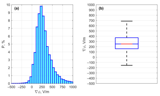
Figure 2.
Histogram of the potential gradient under fair-weather conditions for 2006–2020 in Tomsk (a) and the box-plot quartile diagram (b).
At a 95% confidence level, the minimum and maximum values of ∇φ are 37 and 638 V/m, respectively. The total range of value variability under fair-weather conditions is estimated as a range from Q1 − 1.5 IQR to Q3 + 1.5 IQR, where Q1 and Q3 are the 25th and 75th percentiles, respectively, and IQR has a range of around −155 to 688 V/m. Values of ∇φ, limited to the interval Q1 ÷ Q3, are typical for Tomsk and range from 161 to 372 V/m.
3.2. Diurnal Variations in the Potential Gradient
According to the classification established in [6,13,51], the daily fluctuations in the potential gradient recorded in Tomsk can be attributed to the second type—oscillations of the continental type with a double maximum and double minimum (see Figure 3 and Figure 4, Table A4).
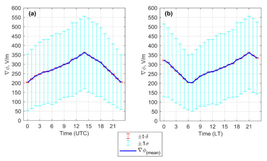
Figure 3.
Hourly mean diurnal variation in the potential gradient under fair-weather conditions, calculated for 2006–2020. On the X-axis, UTC (Panel (a)) and local time (LT) (Panel (b)) are shown. In the figures, the width of the confidence interval ±t⋅δ is determined by the multiplication of the Student’s t-value (t) and the standard error of the mean (δ = σ/√N, where σ—standard deviation, N—sample length), and ±1σ—the range equal to one standard deviation.
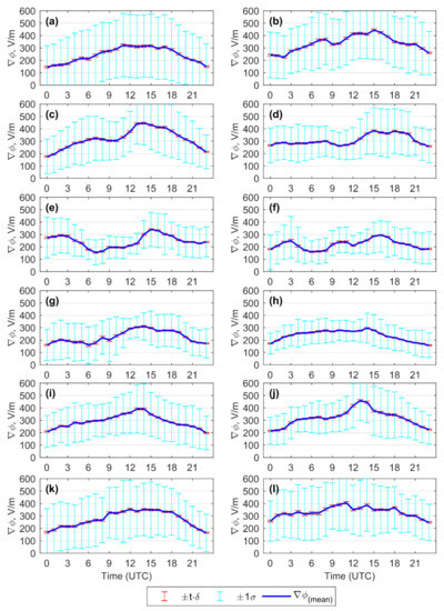
Figure 4.
Hourly mean diurnal variation in the potential gradient under fair-weather conditions, calculated for the specific months: January (a), February (b), March (c), April (d), May (e), June (f), July (g), August (h), September (i), October (j), November (k), December (l). In this figure, the width of the confidence interval ±t⋅δ is determined by the multiplication of the Student’s t-value (t) and the standard error of the mean (δ = σ/√N, where σ—standard deviation, N—sample length), and ±1σ—the range equal to one standard deviation.
As shown in Figure 3, the main minimum of diurnal ∇φ occurs around 00 UTC and the main maximum of diurnal ∇φ occurs at about 14 UTC on average throughout the year. A detailed examination of the main maximum of diurnal ∇φ in different months (see Figure 3) reveals a bimodularity (“double-headed”). This phenomenon is presumably explained by the superposition of local (the maximum of convective instability observing 8–10 UTC at the observation site [60,61,62,63]) and global (the maximum of unitary variation observing 11–13 UTC [1,10]) processes.
Figure 4 demonstrates that, in addition to the prominent main maximum and minimum of diurnal ∇φ, the secondary maximum and minimum of diurnal ∇φ caused by the convective generator [6,7,18] may also be seen in different months. Their manifestation is timed to coincide with the sunrise and varies greatly from summer to winter. Thus, the secondary maximum in July is noted at ~2 UTC, and in February, it occurs at ~8 UTC.
The diurnal ∇φ variation averages approximately 56% of the mean annual value, which is consistent with similar results from other continental observation sites [13,21,51]. The amplitude of diurnal ∇φ changes significantly, exceeds the annual average during the winter months, and can reach 100%.
3.3. Seasonal Variations of the Potential Gradient
On fair-weather days in Tomsk, the intra-annual dynamics of mean monthly values of the potential gradient may be roughly described by a simple wave with a minimum in summer and a maximum in winter (see Figure 5), which generally agrees with comparable estimates [10,13,21]. The variance of ∇φ values also increases significantly from summer to winter.
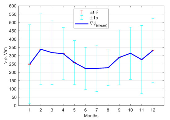
Figure 5.
Seasonal variation in the potential gradient obtained under fair-weather conditions in Tomsk. In the figure, the width of the confidence interval ±t⋅δ is determined by the multiplication of the Student’s t-value (t) and the standard error of the mean (δ = σ/√N, where σ—standard deviation, N—sample length), and ±1σ—the range equal to one standard deviation.
The annual variability in the monthly mean values of ∇φ in Tomsk is 41% of the long-term mean, which agrees with the estimates for the northern hemisphere, equal to 48% [13,21,51].
The seasonal variability in November and January deviates greatly from the general pattern. There is a significant decrease in the monthly mean and diurnal mean values of ∇φ (see Figure 6).
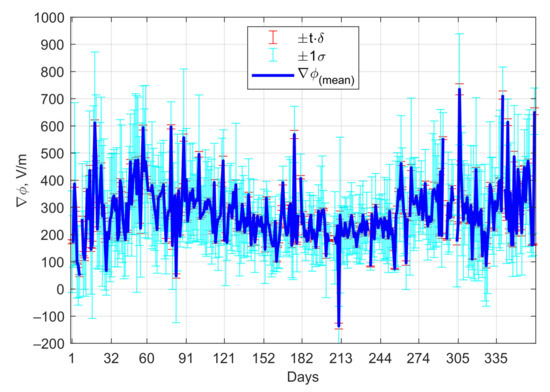
Figure 6.
Hourly mean diurnal variation in the potential gradient under fair-weather conditions in Tomsk, calculated over 2006–2020. In the figure, the width of the confidence interval ±t⋅δ is determined by the multiplication of the Student’s t-value (t) and the standard error of the mean (δ = σ/√N, where σ—standard deviation, N—sample length), and ±1σ—the range equal to one standard deviation.
4. Discussion
Although the potential gradient under fair-weather conditions is well known, the study of long-term datasets for new regions can complement the current understanding of atmospheric electricity, as well as help in predicting future changes.
Variations in background radiation and aerosol air pollution, which are strongly related to changes in air temperature, wind speed, and snow depth (SD), can partially explain the patterns of changes in the potential gradient recorded in Tomsk. For the entire study period, the correlation coefficient at a significance of 95% of monthly averages of the potential gradient with snow depth is 0.58, that with atmospheric transparency at 380 nm is 0.58, that with air temperature is −0.61, that with gamma radiation is −0.61, and that with wind speed is 0.74. The above correlation coefficients indicate significant relationships between the variability in the potential gradient and other quantities. These local factors, in turn, are superimposed on the response of the planetary-scale processes in the electric field associated with the GEC [1,10].
Let us proceed to the interpretation of the seasonal variability registered in Tomsk. The low intensity of air ionization under the influence of radon and its derivatives (minimal gamma radiation) and relatively high atmospheric transparency are likely to be the causes of the winter maximum. The ionizing power of galactic cosmic rays is also minimal due to the high pressure and low temperatures in winter [64]. The reduction in the background radiation during winter is due to soil freezing and a substantial snow cover that prevents radon emission from the soil (see Figure A2). Snow depth also limits soil-derived aerosols in the air. The reduced aerosol concentration at the observation site in winter is also linked to mean wind speeds ~2.6 m/s (see Figure A2e), which causes aerosol export. In winter, high wind speeds <6 m/s caused by advection on the periphery of the Siberian high lead to aerosol export away from the observation site, lowering the concentration value.
In spring-summertime, the opposite picture is observed: as the snow melts, radon emanation rises and gamma radiation increases [64]. The strong surface heating and an upwards by convective mixing promote aerosol air pollution. As a result of these processes, the potential gradient during this period reaches its minimum.
For summer (July as an example), the correlation coefficient at a significance of 95% between hourly average values of the potential gradient and wind speed, gamma radiation, atmospheric transparency at 380 nm, and solar irradiance was −0.25, −0.28, −0.28, and −0.53, respectively.
The diurnal variability can be roughly interpreted as follows: in the night and morning hours, increased ionization of the air (relatively high gamma-radiation) leads to lower potential values. After sunrise, as warming and intensification of convection and turbulent mixing (along with an increase in wind speed), aerosol rises and mixes in the air, resulting in higher levels of aerosol contamination in the surface layer. At this time, mainly in spring and summer, a secondary maximum of the potential gradient is observed (see Figure A3). The intensity of convective motions peaks in the near-afternoon (12–15 LT), while gamma-radiation and aerosol air pollution rapidly decline and reach their lowest levels around 13–15 LT, likely due to the removal of radon and its derivatives from the surface layer. At the same time, air pollution from aerosols is low. In spring and summer, a secondary minimum is noted (see Figure A3). An increase in the potential gradient begins in autumn with lower air temperatures, soil freezing, and snow cover formation.
Solar irradiance changes and, as a consequence, air temperature variations account for much of the diurnal variability of the potential gradient (see Figure A3 and Figure A4). Convective disturbances and turbulent mixing increase with air temperature, contributing to the redistribution of radon and its decay products (radionuclides) as well as aerosol particles in the atmosphere.
As shown in the previous section (see Figure 5 and Figure 6), November is outside of the general trend and shows a strong decrease (~15%) in the potential gradient. A likely explanation is the sharp increase in gamma radiation intensity this month (see Figure A2), but additional research is required to elucidate the reasons.
Aerosol contamination in the ground layer increases and atmospheric transparency decreases after 15 LT due to a gradual weakening of the convective motions and sinking of the aerosols they lift into the ground layer, reaching a maximum around 18–19 LT in the summer (see Figure A3) and 15–16 LT in winter (see Figure A4). There is a gradual increase in the radiation background. The potential gradient grows rapidly as a result of these actions. The combined effect of the local variables outlined above and the global process (unitary variation) forms the major maximum of the potential gradient.
Aerosol [64] and radionuclides [65] deposition occurs after sunset, as well as subsidence of convective and turbulent motions, resulting in a clear transparent atmosphere and increasing background radiation. The latter factor contributes to the decrease in the potential gradient in the surface layer.
Then, we compared our results to the unitary variation (Carnegie curve) and the findings of other researchers for different parts of the globe. The absolute values of the potential gradient, both for specific months and for the entire year, strongly exceed the planetary average (see Figure 7a and Table A4). It is evident that the annual average in ∇φ in Tomsk is twice the Carnegie value. This disparity is explained by placement in a populated area. Furthermore, the presence of snow cover and soil freezing for an average of 7 months a year, which prevents radon emission from the soil, plays a significant part in the increase in the annual average ∇φ values in Tomsk.
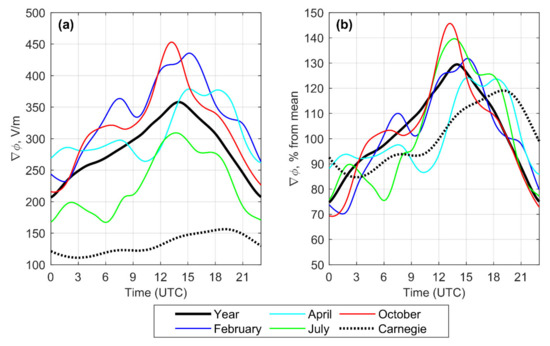
Figure 7.
Smoothed daily variations in absolute (a) and normalized (b) potential gradient under fair-weather conditions (February, April, July, and October and the annual average values calculated for 2006–2020) obtained at Tomsk in comparison with the unitary variation (Carnegie curve [1]).
A comparison of the multiyear mean in Tomsk to similar values obtained at urban observation sites and sites in the interior of the continent revealed their approximate agreement. Thus, the long-term average values in Islamabad (Pakistan) [66], Mitzpe Ramon (Israel) [6], London (UK) [6,41], Muzaffarabad (Pakistan) [67], and Srinagar (India) [68] are about 170, 190, 370, 390, and 470 V/m, respectively.
The diurnal variations in the normalized versus average ∇φ values in Tomsk are generally consistent with the unitary variation. Hourly means of the potential gradient with month of the year in the south of Western Siberia are generally characterized by a minimum in the morning (00 UTC) during summer and a maximum in the evening (14 UTC) during late winter (see Figure 8). However, their primary minimum and maximum are 03 and 05 UTC earlier than a similar one on the Carnegie curve, respectively (see Figure 7b).
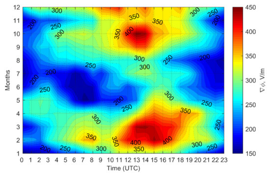
Figure 8.
Hourly means of potential gradient with month of yearunder fair-weather conditions for 2006–2020 in Tomsk.
It should be noted that the diurnal variations observed in Tomsk match the pattern observed in Srinagar, India [68] and the Complejo AStronomico el LEOncito (CASLEO), Argentina [69]. Seasonal variability in Tomsk is comparable to Islamabad, Pakistan [67] and Reading, the United Kingdom [11].
5. Conclusions
New estimates of diurnal and seasonal variability of the potential gradient under fair-weather conditions in the southern part of Western Siberia using Tomsk as an example were obtained:
- The annual average in the potential gradient in Tomsk is 282 V/m, within a range of between 161 and 372 V/m;
- A lognormal distribution describes the variations in potential gradient values in Tomsk under fair weather conditions;
- On average, the diurnal variations in potential gradient per year are characterized by oscillations of the continental type with a double maximum and minimum;
- Variations have a main minimum of 00 UTC and a main maximum of 14 UTC;
- The diurnal variability in potential gradient accounts for around 56% of the annual average value;
- The changes over the course of a day, normalized by the average potential gradient values, are generally consistent with the daily pattern known as the Carnegie curve; however, their minimum and maximum are shifted relative to the curve by an earlier time (by 3 and 5 h, respectively);
- Most of the diurnal variability of the potential gradient in Tomsk is related to variations in global horizontal irradiance and, as a consequence, air temperature variations; convective disturbances and turbulent mixing change as air temperature varies, causing radon and its decay products (radionuclides) as well as aerosol particles to redistribute in the atmosphere;
- The observed diurnal variations in the potential gradient are driven by diurnal changes in radionuclides and aerosol particles;
- The annual variability in monthly average potential gradient values is 41% of the long-term mean;
- According to the annual mode, the maximum potential gradient is observed in February, and the minimum in June;
- The seasonal variations in background radiation and aerosol air pollution, which are strongly related to changes in air temperature, wind speed, and snow cover, can partially explain the patterns of season changes in the potential gradient observed in Tomsk.
Though the absolute values of the potential gradient recorded in Tomsk are only representative of the city (overestimated when compared to those in natural landscapes and rural areas), the observed seasonal and diurnal patterns of the potential gradient are generally correct for the study area.
Author Contributions
Conceptualization, K.P. and P.N.; methodology, K.P., P.N., M.O. and S.S.; software, K.P.; validation, K.P., P.N. and S.S.; formal analysis, K.P.; investigation, K.P.; resources, K.P., P.N. and S.S.; data curation, K.P. and S.S.; writing—original draft preparation, K.P. and M.O.; writing—review and editing, K.P., P.N., M.O. and S.S.; visualization, K.P.; supervision, K.P.; project administration, K.P.; funding acquisition, K.P. All authors have read and agreed to the published version of the manuscript.
Funding
This research is supported by the Russian Science Foundation (Russia), project No.22-27-00482, https://www.rscf.ru/en/project/22-27-00482 (accessed on 4 April 2022).
Institutional Review Board Statement
Not applicable.
Informed Consent Statement
Not applicable.
Data Availability Statement
Not applicable.
Conflicts of Interest
The authors declare no conflict of interest.
Appendix A

Table A1.
Number of potential gradient values (mean per minute) and the total data period under fair-weather conditions and under different weather conditions in Tomsk according to data from the IMCES GO for 2006–2020. Data of potential gradient for 2010 are missing due to the repair and calibration of the field mill in the Voeikov Main Geophysical Observatory (St. Petersburg, Russia).
| Conditions | 2006 | 2007 | 2008 | 2009 | 2010 | 2011 | 2012 | 2013 | 2014 | 2015 | 2016 | 2017 | 2018 | 2019 | 2020 | Sum | |
|---|---|---|---|---|---|---|---|---|---|---|---|---|---|---|---|---|---|
| Number of the potential gradient values, 103 | Fair- weather | 38 | 35 | 17 | 30 | - | 29 | 73 | 45 | 18 | 53 | 85 | 20 | 86 | 64 | 52 | 645 |
| Different- weather | 214 | 312 | 255 | 201 | - | 133 | 448 | 455 | 161 | 302 | 458 | 265 | 495 | 436 | 514 | 4649 | |
| Total data period, days | Fair- weather | 26.4 | 24.3 | 11.8 | 20.8 | - | 20.1 | 50.7 | 31.3 | 12.5 | 36.8 | 59.0 | 13.9 | 59.7 | 44.4 | 36.1 | 447.9 |
| Different- weather | 148.6 | 216.7 | 177.1 | 139.6 | - | 92.7 | 311.1 | 316.0 | 111.8 | 209.7 | 318.1 | 184.0 | 343.8 | 302.8 | 356.9 | 3228.5 | |
Table A2.
Relationship (in%) of the potential gradient values numbers under fair-weather conditions and under different weather conditions in Tomsk according to data from the IMCES GO for 2006–2020. Data of potential gradient for 2010 are missing due to the repair and calibration of the field mill in the Voeikov Main Geophysical Observatory (St. Petersburg, Russia).
| 2006 | 2007 | 2008 | 2009 | 2010 | 2011 | 2012 | 2013 | 2014 | 2015 | 2016 | 2017 | 2018 | 2019 | 2020 | Mean |
|---|---|---|---|---|---|---|---|---|---|---|---|---|---|---|---|
| 17.8 | 11.2 | 6.7 | 14.9 | - | 21.8 | 16.3 | 9.9 | 11.2 | 17.6 | 18.6 | 7.6 | 17.4 | 14.7 | 10.1 | 14.0 |
Table A3.
Statistical parameters of the total variability in the potential gradient under fair-weather conditions in Tomsk according to data from the IMCES GO for 2006–2020.
Table A3.
Statistical parameters of the total variability in the potential gradient under fair-weather conditions in Tomsk according to data from the IMCES GO for 2006–2020.
| Period | Mean, V/m | Standard Deviation, V/m | Median, V/m | Interquartile Range, V/m | 5th Percentile, V/m | 25th Percentile, V/m | 75th Percentile, V/m | 95th Percentile, V/m |
|---|---|---|---|---|---|---|---|---|
| January | 249 | 238 | 197 | 320 | −30 | 60 | 379 | 740 |
| February | 338 | 213 | 299 | 256 | 53 | 195 | 451 | 780 |
| March | 318 | 192 | 300 | 231 | 30 | 193 | 424 | 664 |
| April | 312 | 157 | 281 | 184 | 123 | 203 | 387 | 612 |
| May | 258 | 133 | 234 | 151 | 87 | 176 | 327 | 498 |
| June | 223 | 128 | 212 | 139 | 59 | 139 | 278 | 442 |
| July | 224 | 139 | 227 | 150 | 10 | 146 | 296 | 450 |
| August | 228 | 107 | 214 | 130 | 85 | 154 | 284 | 425 |
| September | 289 | 166 | 263 | 207 | 87 | 169 | 376 | 627 |
| October | 315 | 157 | 284 | 194 | 123 | 203 | 397 | 612 |
| November | 276 | 206 | 245 | 269 | 15 | 120 | 389 | 682 |
| December | 331 | 194 | 300 | 250 | 72 | 193 | 444 | 695 |
| Year | 282 | 182 | 252 | 211 | 37 | 161 | 372 | 638 |
Table A4.
Hourly average values of the potential gradient under fair-weather conditions in Tomsk according to data from the IMCES GO for 2006–2020.
Table A4.
Hourly average values of the potential gradient under fair-weather conditions in Tomsk according to data from the IMCES GO for 2006–2020.
| Time (UTC/LT) | Absolute Values ∇ϕ,V/m | Relative Values ∇ϕ,% of the Mean | Time(UTC/LT) | Absolute Values ∇ϕ,V/m | Relative Values ∇ϕ,% of the Mean |
|---|---|---|---|---|---|
| 00/07 | 203 | 72 | 12/19 | 332 | 118 |
| 01/08 | 221 | 78 | 13/20 | 349 | 123 |
| 02/09 | 239 | 84 | 14/21 | 362 | 128 |
| 03/10 | 248 | 88 | 15/22 | 348 | 123 |
| 04/10 | 259 | 92 | 16/23 | 334 | 118 |
| 05/11 | 262 | 93 | 17/00 | 322 | 114 |
| 06/12 | 269 | 95 | 18/01 | 310 | 110 |
| 07/13 | 280 | 99 | 19/02 | 287 | 101 |
| 08/14 | 287 | 102 | 20/03 | 266 | 94 |
| 09/15 | 299 | 106 | 21/04 | 247 | 87 |
| 10/17 | 305 | 108 | 22/05 | 224 | 79 |
| 11/18 | 325 | 115 | 23/06 | 205 | 72 |

Figure A1.
Histogram of the potential gradient values under differentweather conditions for Tomsk (a) and the Box Plot quartile diagram (b).
Figure A1.
Histogram of the potential gradient values under differentweather conditions for Tomsk (a) and the Box Plot quartile diagram (b).

Table A5.
Statistical parameters of the variability in the potential gradient under different weather conditions in Tomsk according to data from the IMCES GO for 2006–2020.
Table A5.
Statistical parameters of the variability in the potential gradient under different weather conditions in Tomsk according to data from the IMCES GO for 2006–2020.
| Period | Mean, V/m | Standard Deviation, V/m | Median, V/m | Interquartile Range, V/m | 5th Percentile, V/m | 25th Percentile, V/m | 75th Percentile, V/m | 95th Percentile, V/m |
|---|---|---|---|---|---|---|---|---|
| January | 202 | 355 | 164 | 277 | −184 | 30 | 307 | 712 |
| February | 217 | 327 | 203 | 285 | −197 | 72 | 357 | 721 |
| March | 164 | 478 | 191 | 263 | −307 | 45 | 307 | 574 |
| April | 187 | 899 | 229 | 218 | −316 | 124 | 342 | 606 |
| May | 124 | 1043 | 205 | 213 | −525 | 101 | 314 | 555 |
| June | 180 | 838 | 211 | 160 | −87 | 131 | 292 | 484 |
| July | 177 | 787 | 207 | 187 | −117 | 121 | 307 | 515 |
| August | 196 | 717 | 214 | 161 | −56 | 139 | 300 | 493 |
| September | 163 | 629 | 188 | 191 | −176 | 102 | 293 | 511 |
| October | 168 | 738 | 180 | 229 | −300 | 63 | 293 | 580 |
| November | 214 | 553 | 169 | 257 | −203 | 53 | 310 | 735 |
| December | 174 | 347 | 161 | 263 | −212 | 30 | 293 | 614 |
| Year | 180 | 680 | 195 | 221 | −218 | 86 | 307 | 588 |

Figure A2.
Variations in monthly averages of the potential gradient (a), air temperature (b), relative humidity (c), gamma radiation (d), wind speed (e), and atmospheric transparency at 380 nm (f) under fair-weather conditions in Tomsk according to data from the IMCES GO for 2006–2020, and monthly average snow depth (g) according to Tomsk weather station.


Figure A3.
Variations in hourly averages of the potential gradient (a), air temperature (b), relative humidity (c), gamma radiation (d), wind speed (e), atmospheric transparency at 380 nm (f), and solar irradiance (g) under fair-weather conditions during July in Tomsk according to data from the IMCES GO for 2006–2020.


Figure A4.
Variations in hourly averages of the potential gradient (a), air temperature (b), relative humidity (c), gamma radiation (d), wind speed (e), atmospheric transparency at 380 nm (f), and solar irradiance (g) under fair-weather conditions during February in Tomsk according to data from the IMCES GO for 2006–2020.

References
- Harrison, R.G. The Carnegie Curve. Surv. Geophys. 2013, 34, 209–232. [Google Scholar] [CrossRef]
- Nicoll, K.A.; Harrison, R.G.; Barta, V.; Bor, J.; Brugge, R.; Chillingarian, A.; Chum, J.; Georgoulias, A.K.; Guha, A.; Kourtidis, K.; et al. A global atmospheric electricity monitoring network for climate and geophysical research. J. Atmos. Terr. Phys. 2019, 184, 18–29. [Google Scholar] [CrossRef]
- Anisimov, S.V.; Afinogenov, K.V.; Shikhova, N. Dynamics of undisturbed midlatitude atmospheric electricity: From observations to scaling. Radiophys. Quantum Electron. 2014, 56, 709–722. [Google Scholar] [CrossRef]
- Toropov, A.A.; Kozlov, V.I.; Karimov, R.R. Variations of the Atmospheric Electric Field by Observations in Yakutsk. Arct. Subarct. Nat. Resour. 2016, 2, 58–65. (In Russian) [Google Scholar]
- Smirnov, S. Annual variation of atmospheric electricity diurnal variation maximum in Kamchatka. EPJ Web Conf. 2021, 254, 01001. [Google Scholar] [CrossRef]
- Yaniv, R.; Yair, Y.; Price, C.; Katz, S. Local and global impacts on the fair-weather electric field in Israel. Atmos. Res. 2016, 172–173, 119–125. [Google Scholar] [CrossRef]
- Smirnov, S.E. Influence of a convective generator on the diurnal behavior of the electric field strength in the near-earth atmosphere in Kamchatka. Geomagn. Aeron. 2013, 53, 515–521. [Google Scholar] [CrossRef]
- Lopes, F.; Silva, H.G.; Bennett, A.J.; Reis, A.H. Global Electric Circuit research at Graciosa Island (ENA-ARM facility): First year of measurements and ENSO influences. J. Electrost. 2017, 87, 203–211. [Google Scholar] [CrossRef]
- Silva, H.G.; Conceição, R.; Melgão, M.; Nicoll, K.; Mendes, P.B.; Tlemçani, M.; Reis, A.H.; Harrison, R.G. Atmospheric electric field measurements in urban environment and the pollutant aerosol weekly dependence. Environ. Res. Lett. 2014, 9, 114025. [Google Scholar] [CrossRef]
- Bennett, A.J.; Harrison, R.G. Variability in surface atmospheric electric field measurements. J. Phys. Conf. Ser. 2008, 142, 012046. [Google Scholar] [CrossRef]
- Bennett, A.J.; Harrison, R.G. Atmospheric electricity in different weather conditions. Weather 2007, 62, 277–283. [Google Scholar] [CrossRef]
- Hoppel, W.A. Theory of the electrode effect. J. Atmos. Terr. Phys. 1967, 29, 708–721. [Google Scholar]
- Israël, H. Atmospheric Electricity: Atmosphèarische Elektrizitèat; National Technical Information Service; US Department of Commerce: Springfield, VA, USA, 1970.
- Hoppel, W.A.; Frick, G.M. Ion-aerosol attachment coefficients and the steady state charge distribution on aerosols in a bipolar ion environment. Aerosol Sci. Technol. 1986, 5, 1–21. [Google Scholar] [CrossRef]
- Kupovykh, G.V.; Morozov, V.N.; Shvarts, Y.M. Theory of the Electrode Effect in the Atmosphere; TSURE Publishing: Taganrog, Russia, 1998. (In Russian) [Google Scholar]
- Petrov, A.I.; Petrova, G.G.; Panchishkina, I.N. Profiles of polar conductivities and radon-222 concentration in the atmosphere by stable and labile stratification of surface layer. Atmos. Res. 2009, 91, 206–214. [Google Scholar] [CrossRef]
- Morozov, V.N.; Kupovich, G.V. Theory of Electrical Phenomena in Atmosphere; Lap Lambert Academic Publishing: Saarbruken, Germany, 2012. [Google Scholar]
- Anisimov, S.V.; Galichenko, S.V.; Shikhova, N.M.; Afinogenov, K.V. Electricity of the convective atmospheric boundary layer: Field observations and numerical simulation. Izv. Atmos. Ocean. Phys. 2014, 50, 390–398. [Google Scholar] [CrossRef]
- Adzhiev, A.K.; Kupovykh, G.V. Measurements of the Atmospheric Electric Field under High-Mountain Conditions in the Vicinity of Mt. Elbrus. Izv. Atmos. Ocean. Phys. 2015, 51, 633–638. [Google Scholar] [CrossRef]
- Anisimov, S.V.; Galichenko, S.V.; Mareev, E.A. Electrodynamic properties and height of atmospheric convective boundary layer. Atmos. Res. 2017, 194, 119–129. [Google Scholar] [CrossRef]
- Krasnogorskaia, N.V. Electricity of the Lower Layers of the Atmosphere and Methods of Its Measurement; Gidrometeoizdat: Leningrad, Russia, 1972. (In Russian) [Google Scholar]
- Filippov, A.K. Thunderstorms in Eastern Siberia; Gidrometeoizdat: Leningrad, Russia, 1974. (In Russian) [Google Scholar]
- Rakov, V.A.; Uman, M.A. Lightning: Physics and Effects; Cambridge University Press: New York, NY, USA, 2003. [Google Scholar]
- Popov, I.B. Statistical estimations of various of different meteorological phenomena influence on atmospheric electrical potential gradient. Proc. Voeikov Main Geophys. Obs. 2008, 558, 152–161. (In Russian) [Google Scholar]
- Kamra, A.K. Effect of electric field on charge separation by the falling precipitation mechanism in thunderclouds. J. Atmos. Sci. 1970, 27, 1182–1185. [Google Scholar] [CrossRef][Green Version]
- Illingworth, A.J.; Latham, J. Calculations of electric field growth, field structure and charge distributions in thunderstorms. Q. J. R. Meteorol. Soc. 1977, 103, 281–295. [Google Scholar] [CrossRef]
- Chauzy, S.; Raizonville, P. Space charge layers created by coronae at ground level below thunderclouds: Measurements and modeling. J. Geophys. Res. 1982, 87, 3143–3148. [Google Scholar] [CrossRef]
- Chauzy, S.; Médale, J.C.; Prieur, S.; Soula, S. Multilevel measurement of the electric field underneath a thundercloud: 1. A new system and the associated data processing. J. Geophys. Res. 1991, 96, 22319–22326. [Google Scholar] [CrossRef]
- Petersen, W.A.; Rutledge, S.A. On the relationship between cloud-to-ground lightning and convective rainfall. J. Geophys. Res. Atmos. 1998, 103, 14025–14040. [Google Scholar] [CrossRef]
- Stolzenburg, M.; Marshall, T.C. Charged precipitation and electric field in two thunderstorms. J. Geophys. Res. Atmos. 1998, 103, 19777–19790. [Google Scholar] [CrossRef]
- Lang, T.J.; Rutledge, S.A. Relationships between convective storm kinematics, precipitation, and lightning. Mon. Weather Rev. 2002, 130, 2492–2506. [Google Scholar] [CrossRef]
- Soula, S.; Chauzy, S.; Chong, M.; Coquillat, S.; Georgis, J.-F.; Seity, Y.; Tabary, P. Surface precipitation electric current produced by convective rains during the Mesoscale Alpine Program. J. Geophys. Res. 2003, 108, 4395. [Google Scholar] [CrossRef]
- Liou, Y.-A.; Kar, S.K. Study of cloud-to-ground lightning and precipitation and their seasonal and geographical characteristics over Taiwan. Atmos. Res. 2010, 95, 115–122. [Google Scholar] [CrossRef]
- Klimenko, V.V.; Mareev, E.A.; Shatalina, M.V.; Shlyugaev, Y.V.; Sokolov, V.V.; Bulatov, A.A.; Denisov, V.P. On statistical characteristics of electric fields of the thunderstorm clouds in the atmosphere. Radiophys. Quantum Electron. 2014, 56, 778–787. [Google Scholar] [CrossRef]
- Nagorsky, P.M.; Smirnov, S.V.; Pustovalov, K.N.; Morozov, V.N. Electrode layer in the electric field of deep convective cloudiness. Radiophys. Quantum Electron. 2014, 56, 769–777. [Google Scholar] [CrossRef]
- Pustovalov, K.N.; Nagorskiy, P.M. Response in the surface atmospheric electric field to the passage of isolated air mass cumulonimbus clouds. J. Atmos. Solar Terr. Phys. 2018, 172, 33–39. [Google Scholar] [CrossRef]
- Pustovalov, K.N.; Nagorskiy, P.M. Comparative Analysis of Electric State of Surface Air Layer during Passage of Cumulonimbus Clouds in Warm and Cold Seasons. Atmos. Ocean. Opt. 2018, 31, 685–689. [Google Scholar] [CrossRef]
- Bernard, M.; Underwood, S.J.; Berti, M.; Simoni, A.; Gregoretti, C. Observations of the atmospheric electric field preceding intense rainfall events in the Dolomite Alps near Cortina d’Ampezzo, Italy. Meteorol. Atmos. Phys. 2019, 132, 99–111. [Google Scholar] [CrossRef]
- Whipple, F.J.W. On the association of the diurnal variation of electric potential gradient in fine weather with the distribution of thunderstorms over the globe. Quart. J. R. Met. Soc. 1929, 55, 1–17. [Google Scholar] [CrossRef]
- De, S.S.; Paul, S.; Barui, S.; Pal, P.; Bandyopadhyay, B.; Kala, D.; Ghosh, A. Studies on the seasonal variation of atmospheric electricity parameters at a tropical station in Kolkata, India. J. Atmos. Sol. Terr. Phys. 2013, 105, 135–141. [Google Scholar] [CrossRef]
- Harrison, R.G. Urban smoke concentrations at Kew, London, 1898–2004. Atmos. Environ. 2006, 40, 3327–3332. [Google Scholar] [CrossRef]
- Pkhalagov, Y.A.; Uzhegov, V.N.; Ippolitov, I.I.; Vinarskii, M.V. Investigation of relations between optical and electric characteristics of the surface atmosphere. Opt. Atmos. Okeana 2005, 18, 373–377. (In Russian) [Google Scholar]
- Daskalopoulou, V.; Mallios, S.A.; Ulanowski, Z.; Hloupis, G.; Gialitaki, A.; Tsikoudi, I.; Tassis, K.; Amiridis, V. The electrical activity of Saharan dust as perceived from surface electric field observations. Atmos. Chem. Phys. 2021, 21, 927–949. [Google Scholar] [CrossRef]
- Franzese, G.; Esposito, F.; Lorenz, R.; Silvestro, S.; Popa, C.I.; Molinaro, R.; Cozzolino, F.; Molfese, C.; Marty, L.; Deniskina, N. Electric properties of dust devils. Earth Planet. Sci. Lett. 2018, 493, 71–81. [Google Scholar] [CrossRef]
- Firstov, P.P.; Akbashev, R.R.; Zharinov, N.A.; Maximov, A.; Manevich, T.; Melnikov, T.D. Electric charging of eruptive clouds from Shiveluch Volcano caused by different types of explosions. J. Volcanol. Seismol. 2019, 13, 172–184. [Google Scholar] [CrossRef]
- Wright, M.D.; Matthews, J.C.; Silva, H.G.; Bacak, A.; Percival, C.; Shallcross, D.E. The relationship between aerosol concentration and atmospheric potential gradient in urban environments. Sci. Total Environ. 2019, 716, 134959. [Google Scholar] [CrossRef]
- Davydenko, S.S.; Mareev, E.A.; Marshall, T.C.; Stolzenburg, M. On the calculation of electric fields and currents of mesoscale convective systems. J. Geophys. Res. 2004, 109, D11103. [Google Scholar] [CrossRef]
- Soula, S.; Georgis, J.F. Surface electrostatic field below weak precipitation and stratiform regions of mid-latitude storms. Atmos. Res. 2013, 132–133, 264–277. [Google Scholar] [CrossRef]
- Wilson, J.G.; Cummins, K.L. Thunderstorm and fair-weather quasi-static electric fields over land and ocean. Atmos. Res. 2021, 257, 105618. [Google Scholar] [CrossRef]
- Toropov, A.; Starodubtzev, S.; Kozlov, V. Strong variations of gamma-ray and atmospheric electric field during various meteorological conditions by observations in Yakutsk and Tiksi. Sol.-Terr. Relat. Phys. Earthq. Precursors 2018, 62, 01013. [Google Scholar] [CrossRef]
- Imyanitov, I.M.; Chubarina, E.V. Electricity of the Free Atmosphere; Israel Program for Scientific Translations Ltd.: Jerusalem, Israel, 1967. [Google Scholar]
- Geophysical Observatory, IMCES SB RAS (GO IMCES). Available online: http://www.imces.ru/index.php?rm=news&action=view&id=899 (accessed on 13 February 2022).
- NOAA. ETOPO2. Available online: https://www.ngdc.noaa.gov/mgg/global/relief/ETOPO2/ (accessed on 13 February 2022).
- The Federal State Budgetary Institution “Voeikov Main Geophysical Observatory” (FGBI “MGO”). Available online: http://voeikovmgo.ru/?lang=en&Itemid=136 (accessed on 3 March 2022).
- ALL-Pribors.ru. Available online: https://all-pribors.ru/docs/55005-13.pdf (accessed on 3 March 2022).
- Campbell Scientific. CS110 Electric Field Meter Sensor. Available online: https://www.campbellsci.com/cs110 (accessed on 3 March 2022).
- CS110 Electric Field Meter: Instruction Manual; Campbell Scientific, Inc.: Logan, UT, USA, 2011.
- Russian GOST: Official Regulatory Library. RD 52.04.168-2017. Available online: https://www.russiangost.com/p-372569-rd-5204168-2017.aspx (accessed on 3 March 2022).
- All-Russian Scientific Research Institute of Hydrometeorological Information—World Data Center (VNIIGMI-WDC). Available online: http://meteo.ru/data/ (accessed on 13 February 2022).
- Gorbatenko, V.P.; Konstantinova, D.A. Convection in the atmosphere above south-east of the Western Siberia. Opt. Atmos. I Okeana 2009, 22, 17–21. (In Russian) [Google Scholar]
- Gorbatenko, V.P.; Nechepurenko, O.E.; Krechetova, S.Y.; Belikova, M.Y. The comparison of atmospheric instability indices retrieved from the data of radio sounding and MODIS spectroradiometer on thunderstorm days over West Siberia. Russ. Meteorol. Hydrol. 2015, 40, 289–295. [Google Scholar] [CrossRef]
- Nechepurenko, O.E.; Gorbatenko, V.P.; Konstantinova, D.A.; Sevastyanov, V.V. Instability indices and their thresholds for the forecast of thunderstorms over Siberia. Hydrometeorol. Res. Forecast. 2018, 2, 44–59. (In Russian) [Google Scholar]
- Gorbatenko, V.P.; Kuzhevskaya, I.V.; Pustovalov, K.N.; Chursin, V.V.; Konstantinova, D.A. Assessment of atmospheric convective potential variability in Western Siberia in changing climate. Russ. Meteorol. Hydrol. 2020, 45, 360–367. [Google Scholar] [CrossRef]
- Ryabkina, X.; Kondratyeva, A.; Nagorskiy, P.; Yakovleva, V. Investigation of seasonal dynamics of β- and γ–radiation fields vertical profile in the surface atmospheric layer. IOP Conf. Ser. Mater. Sci. Eng. 2019, 135, 012036. [Google Scholar]
- Kondratyeva, A.G.; Yakovleva, V.S.; Nagorsky, P.M.; Stepanenko, A.A. Dependences in ground atmosphere radon, thoron and decay products dynamics. J. Ind. Pollut. Control. 2016, 32, 397–400. [Google Scholar]
- Gurmani, S.F.; Ahmad, N.; Tacza, J.; Iqbal, T. First seasonal and annual variations of atmospheric electric field at a subtropical station in Islamabad, Pakistan. J. Atmos. Sol. Terr. Phys. 2018, 179, 441–449. [Google Scholar] [CrossRef]
- Ahmad, N.; Gurmani, S.F.; Basit, A.; Shah, M.A.; Iqbal, T. Impact of local and global factors and meteorological parameters in temporal variation of atmospheric potential gradient. Adv. Space Res. 2021, 67, 2491–2503. [Google Scholar] [CrossRef]
- Afreen, S.; Victor, N.J.; Bashir, G.; Chandra, S.; Ahmed, N.; Siingh, D.; Singh, R.P. First observation of atmospheric electric field at Kashmir valley North Western Himalayas, Srinagar (India). J. Atmos. Sol. Terr. Phys. 2020, 211, 105481. [Google Scholar] [CrossRef]
- Tacza, J.; Raulin, J.-P.; Morales, C.A.; Macotela, E.; Marun, A.; Fernandez, G. Analysis of long-term potential gradient variations measured in the Argentinian Andes. Atmos. Res. 2021, 248, 105200. [Google Scholar] [CrossRef]


Publisher’s Note: MDPI stays neutral with regard to jurisdictional claims in published maps and institutional affiliations. |
© 2022 by the authors. Licensee MDPI, Basel, Switzerland. This article is an open access article distributed under the terms and conditions of the Creative Commons Attribution (CC BY) license (https://creativecommons.org/licenses/by/4.0/).