
Development of Vehicle Emission Model Based on Real-Road Test and Driving Conditions in Tianjin, China

Abstract
:1. Introduction
2. Materials and Methods
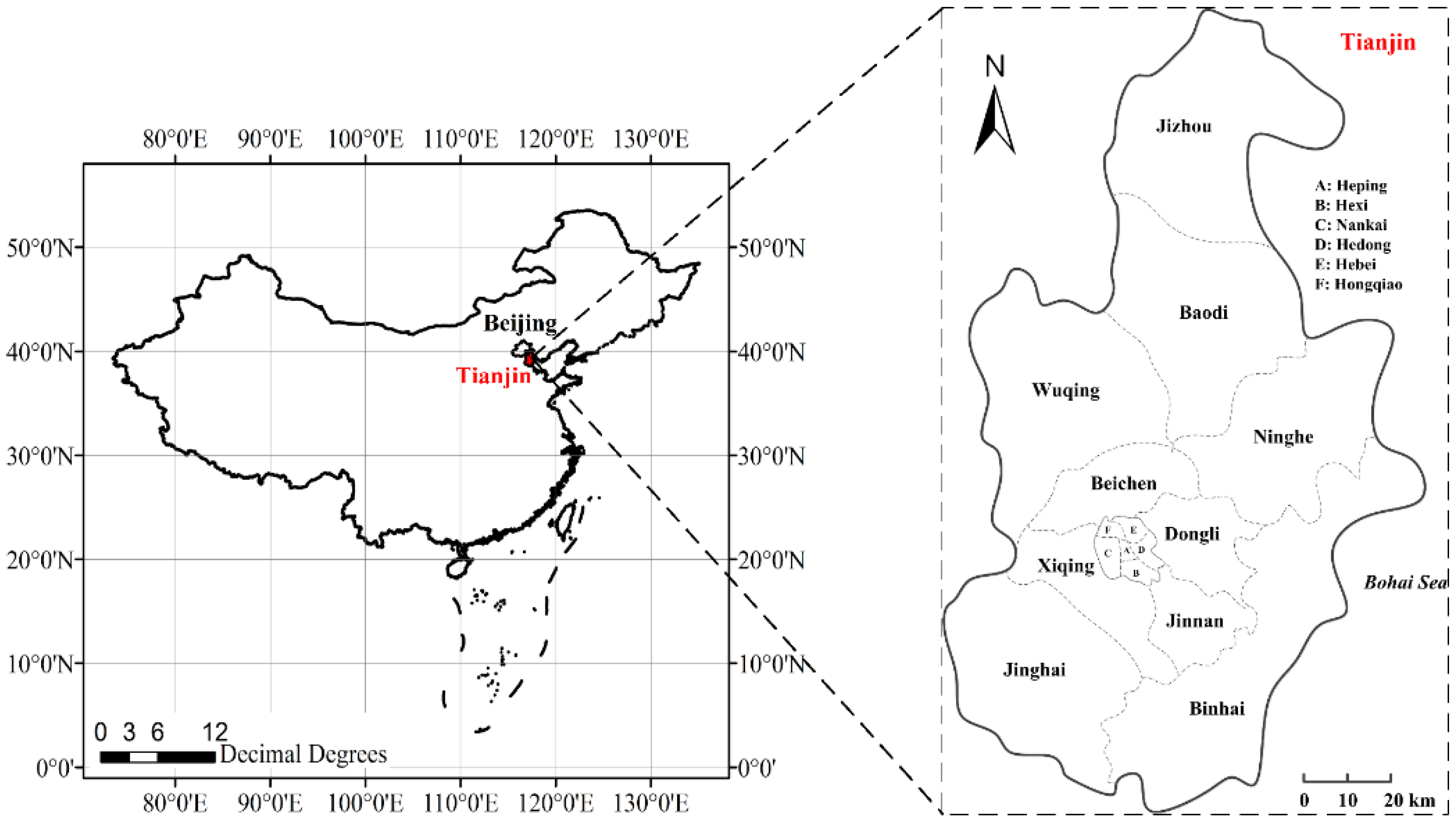
2.1. Study Area
2.2. Modeling Method of Vehicle Emission
2.2.1. Surrogate Variables
- VSP
- VSP interval (VSP-bin)
2.2.2. Generation of Driving Cycle
- Selection of alternative driving cycle
- Calculation of judgment criteria
- Evaluation of coincidence degree
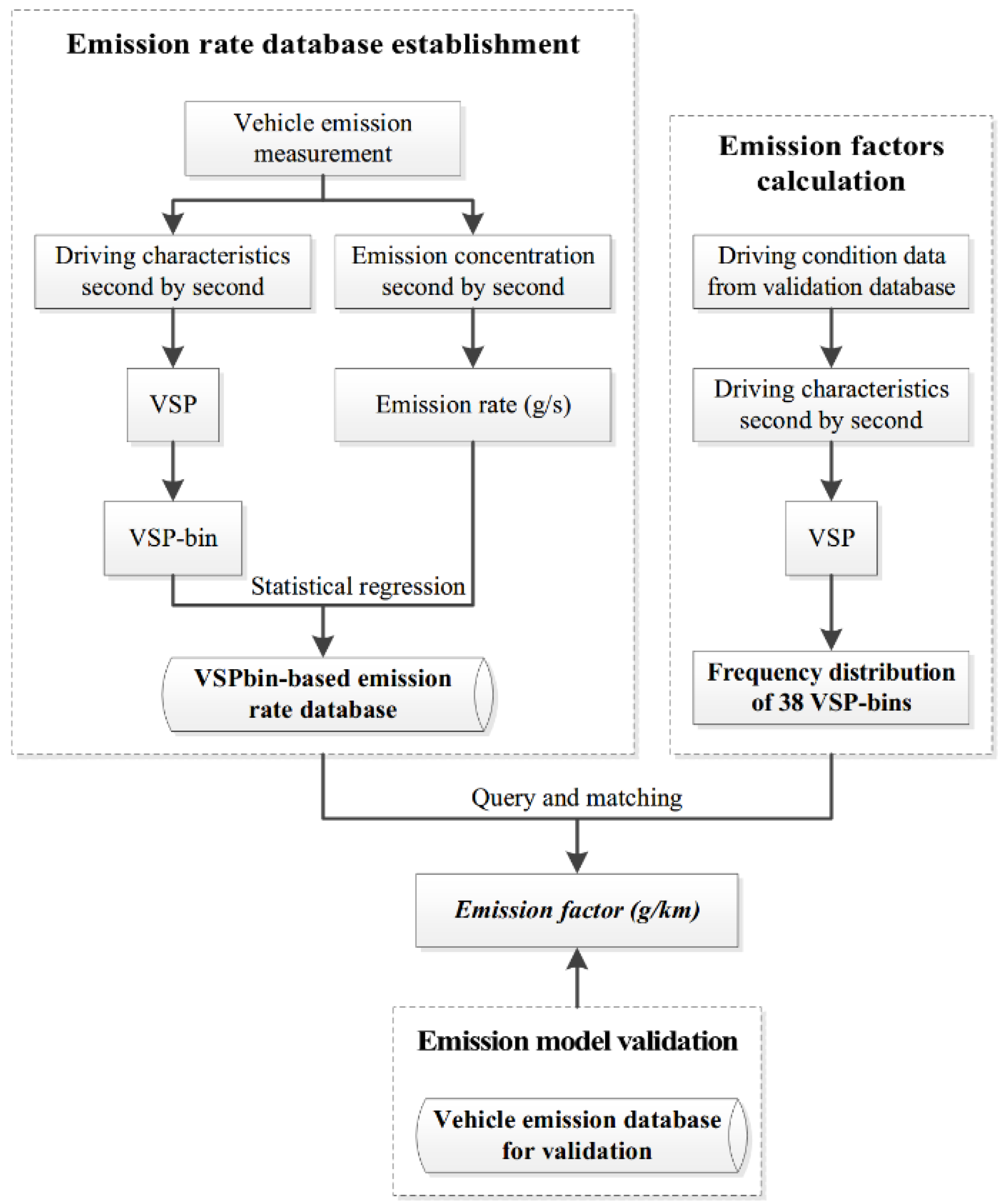
2.2.3. Modeling Steps
- Establishment of emission rate database
- Calculation of emission factor:
- Validation of emission factor
2.3. Real Road Measurement of Vehicle Emission
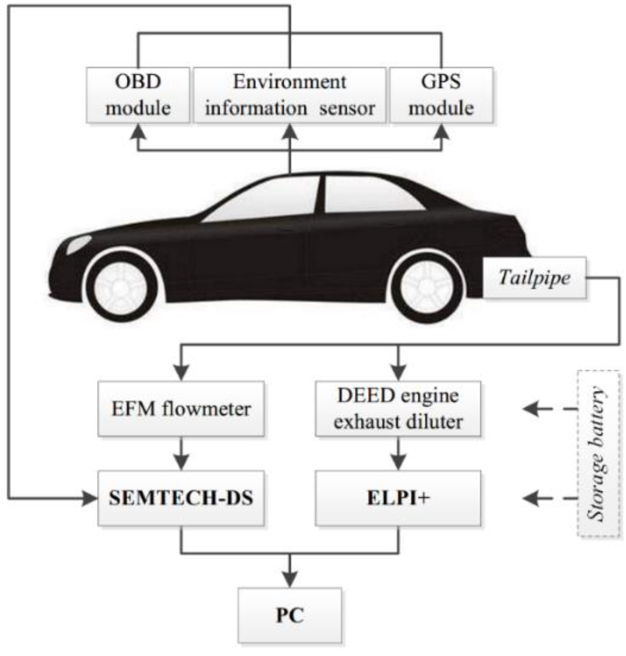
2.3.1. PEMS Establishment
2.3.2. Experimental Design
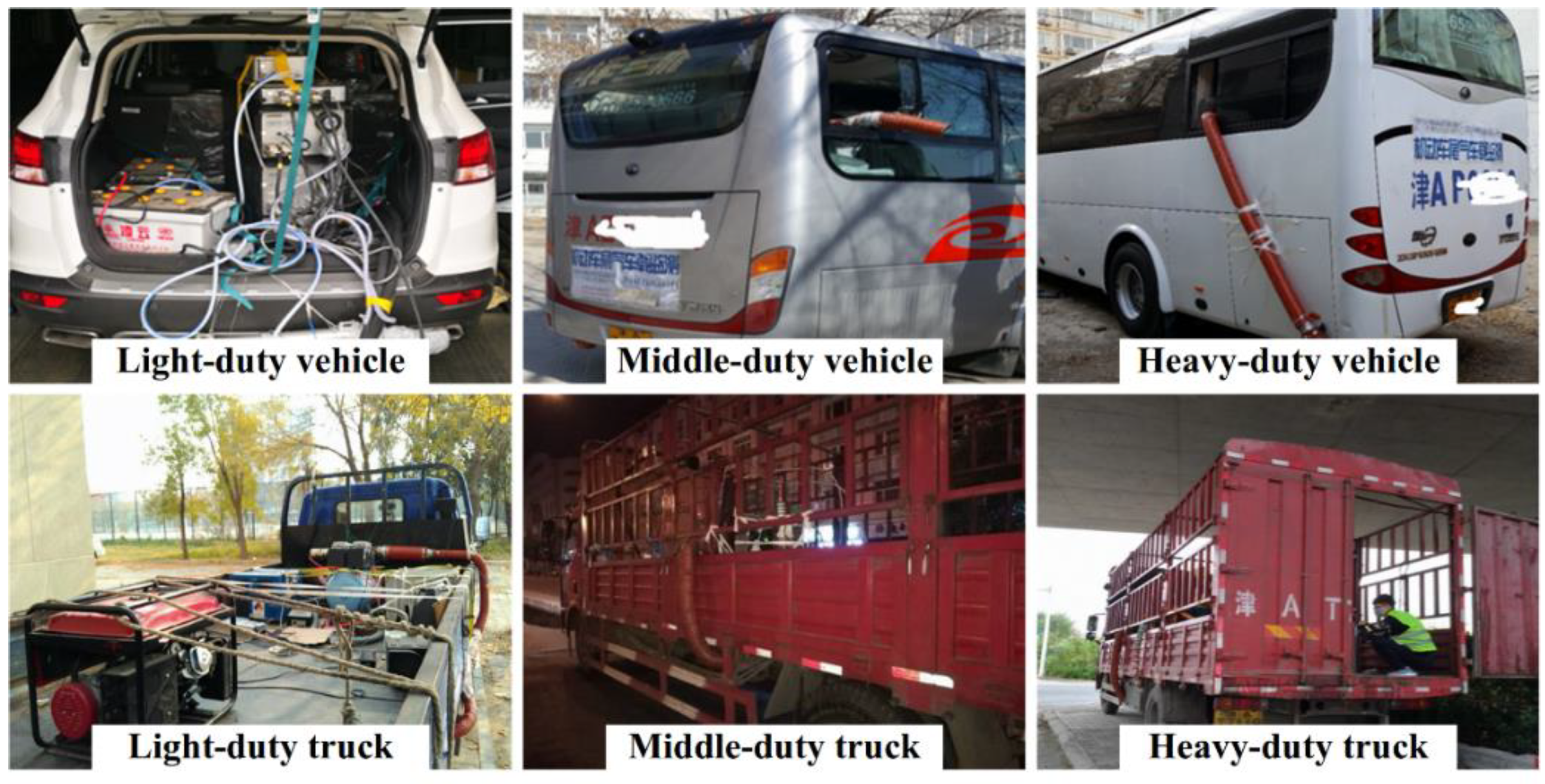
- Tested vehicle
- Test period
- Test indicators
- Driver selection
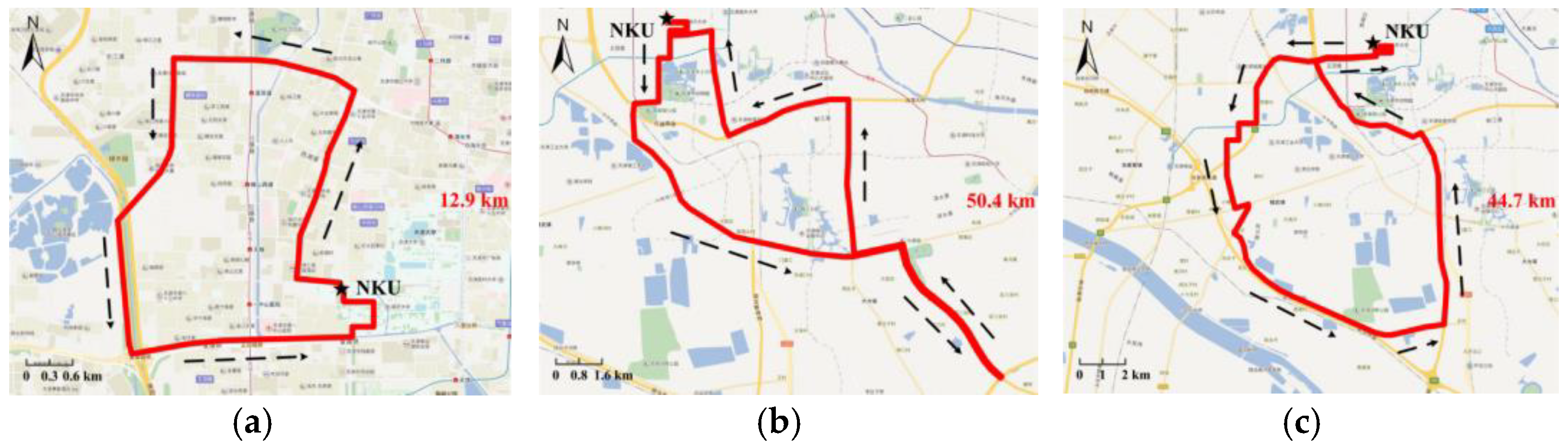
- Test routes
3. Results and Discussion
3.1. Analysis of Vehicle Emission Measurement Results
3.1.1. Relationship between Driving Condition and Emission Rate
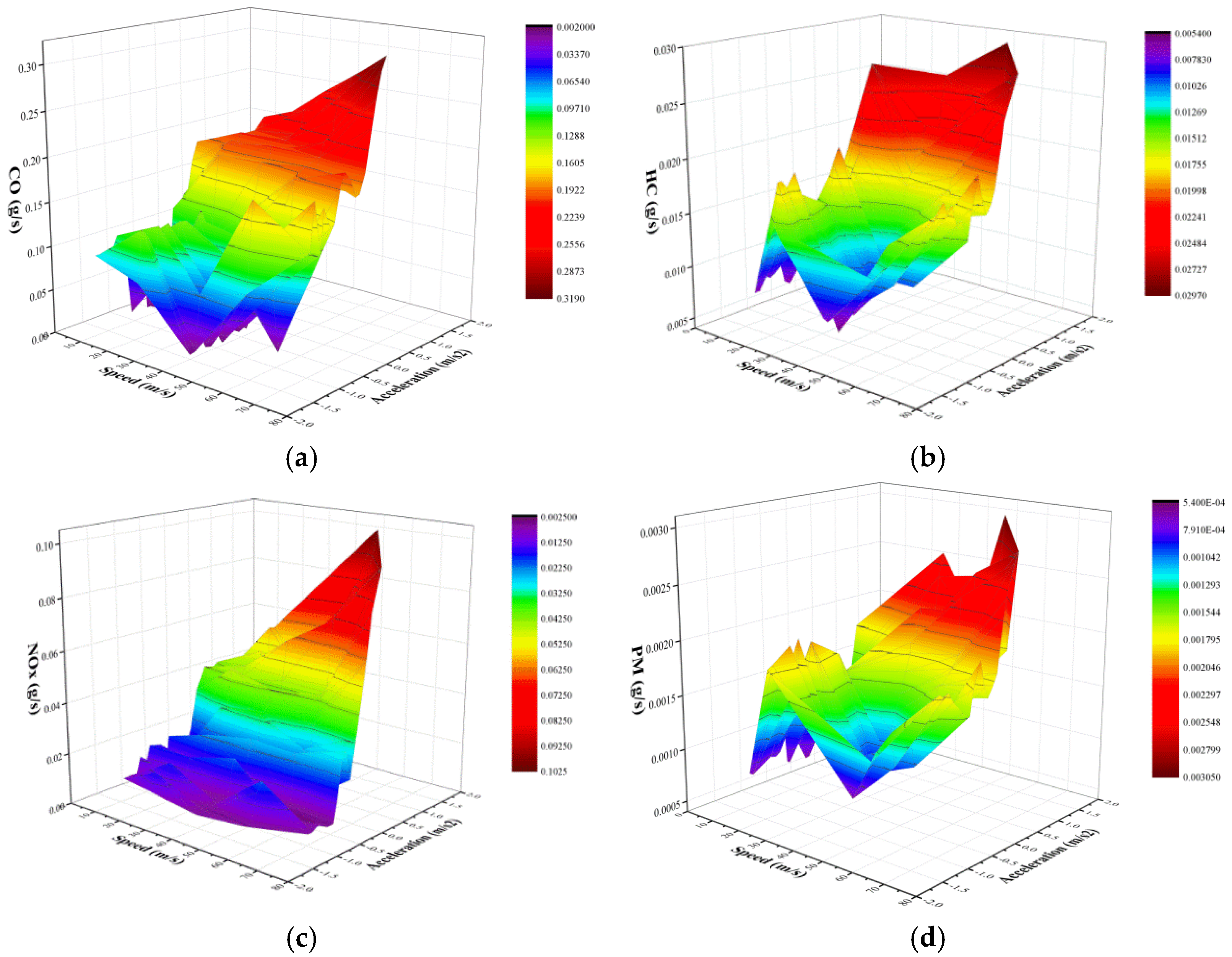
- Relationship between vehicular speed, acceleration and pollutant emission rate
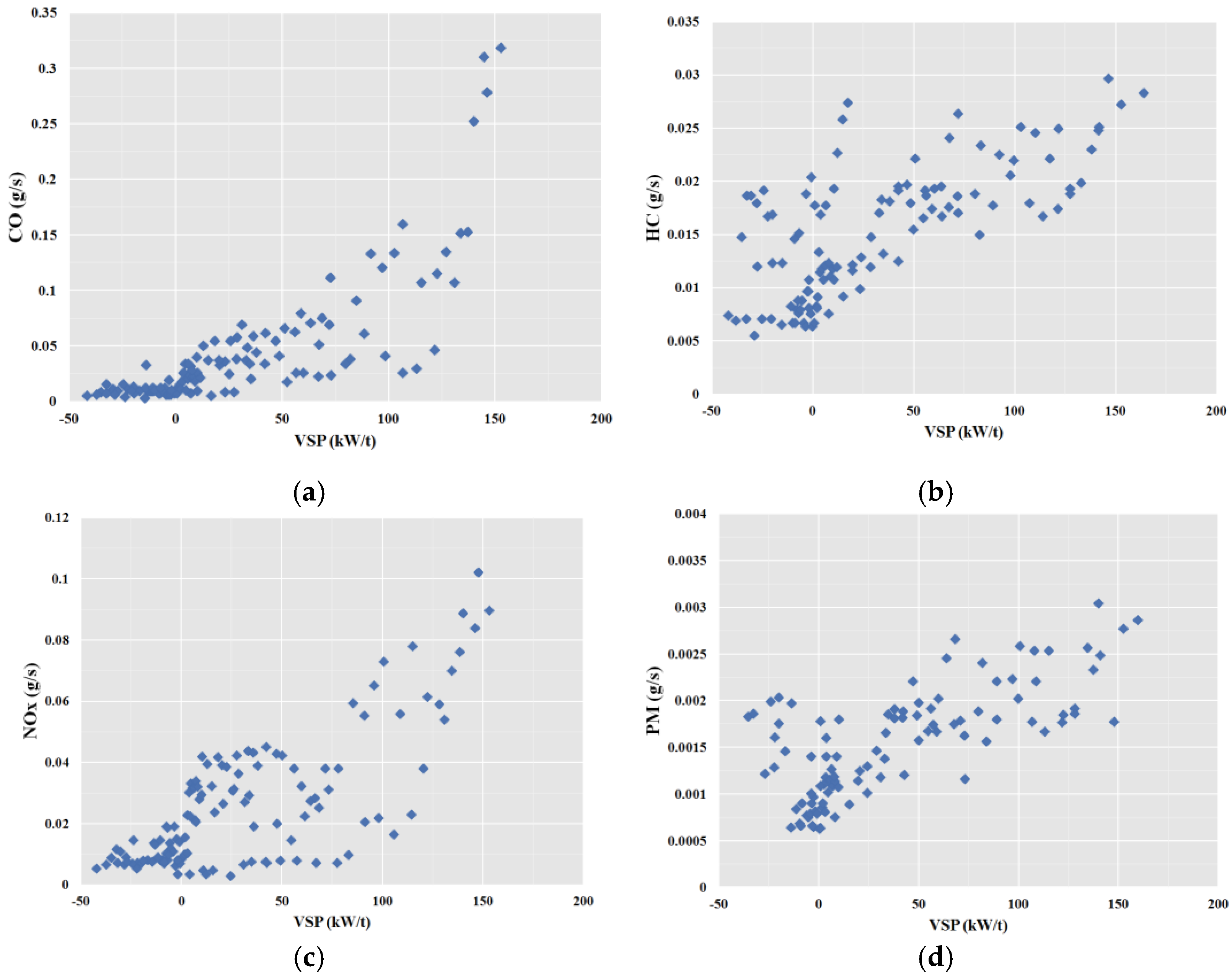
- Relationship between vehicular VSP and pollutant emission rate
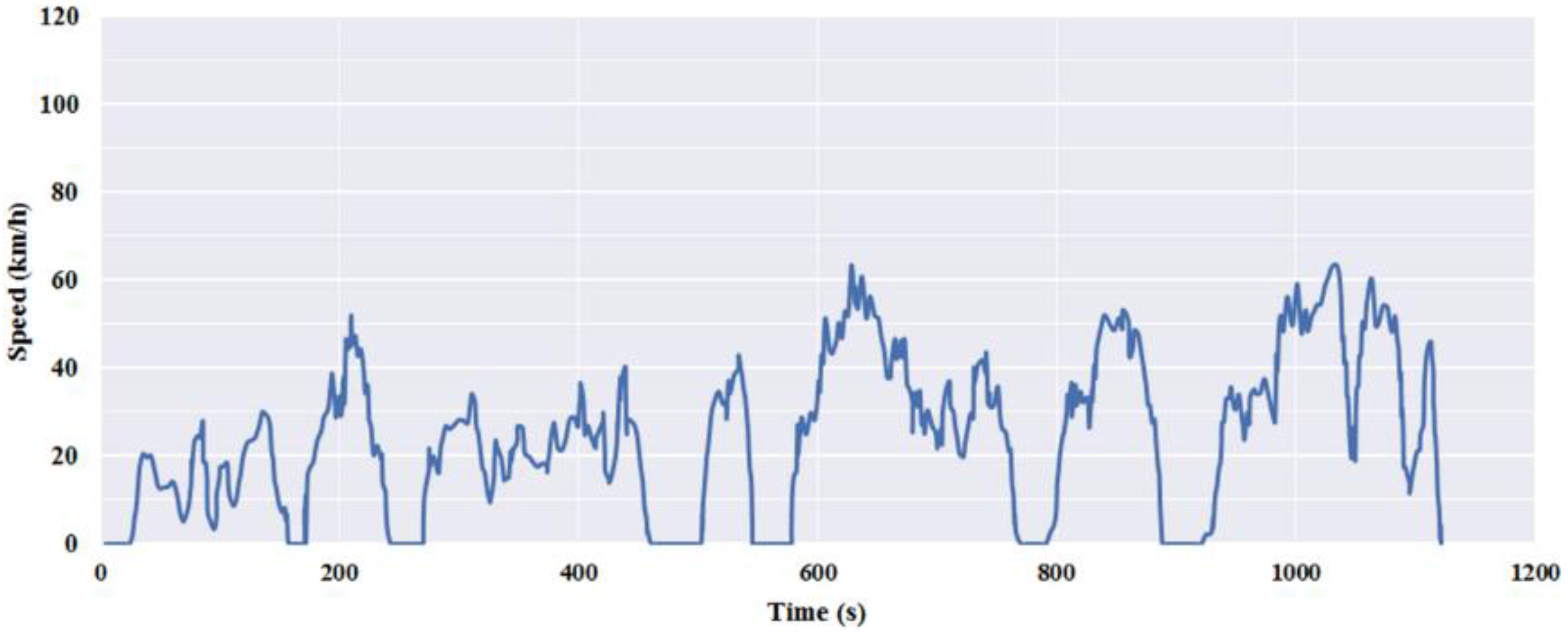
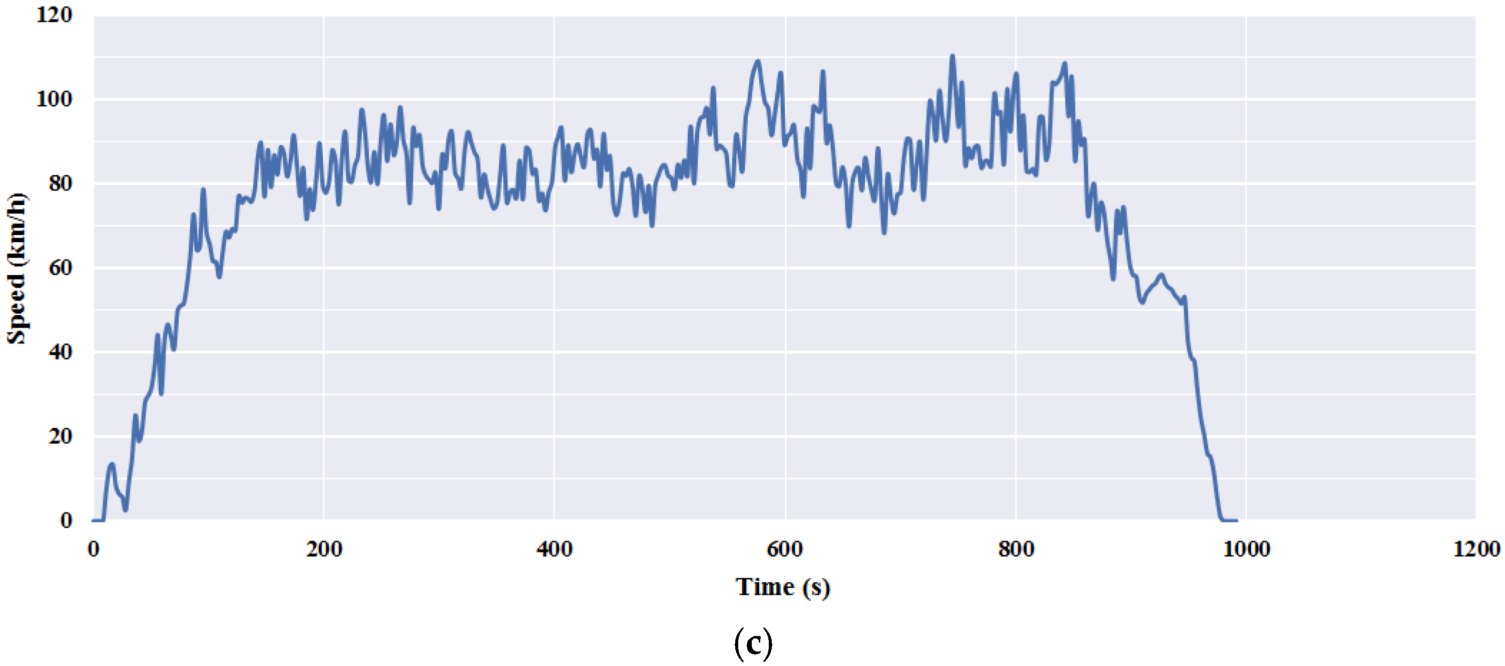
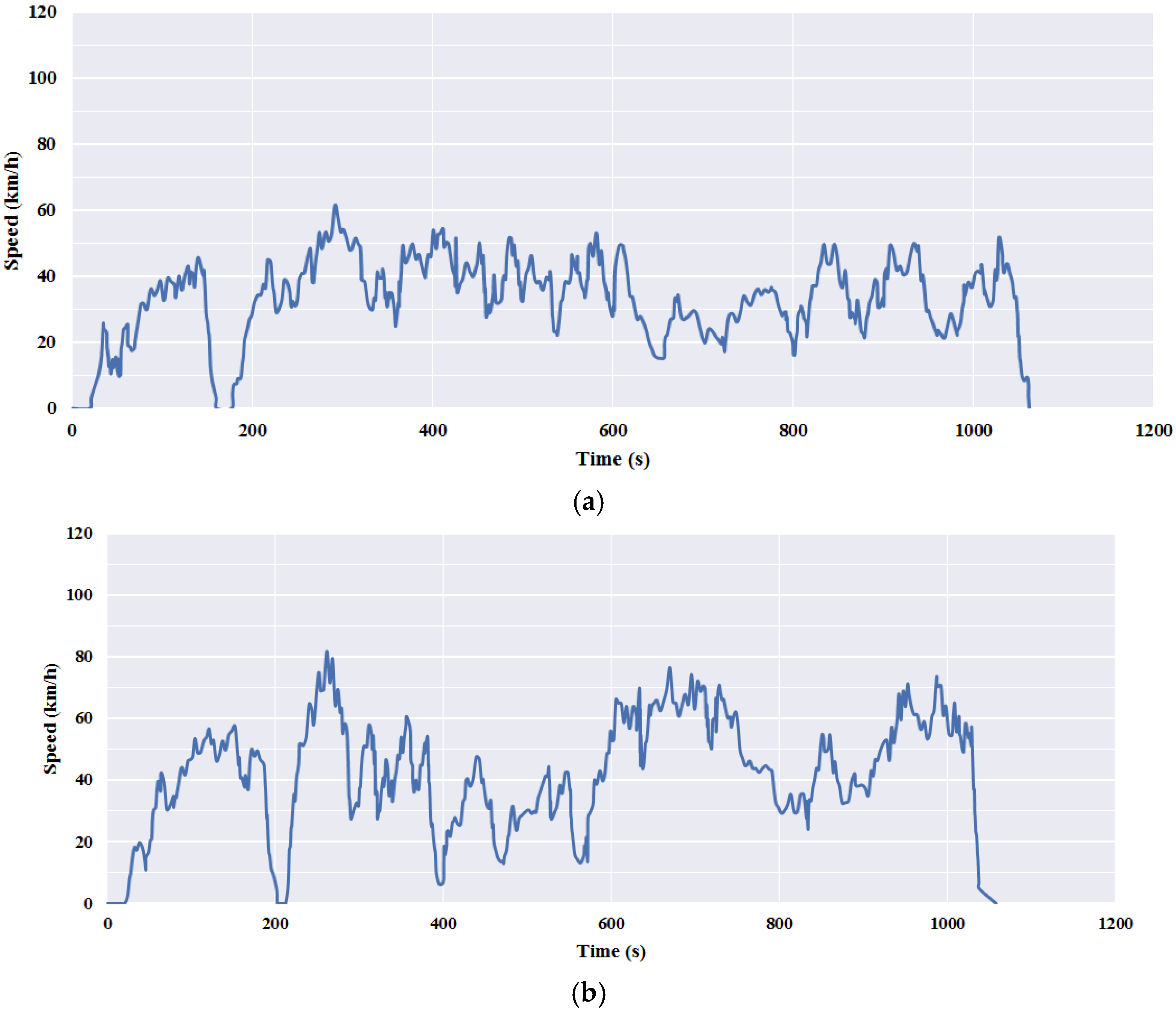
3.1.2. Generation of Localized Driving Cycle
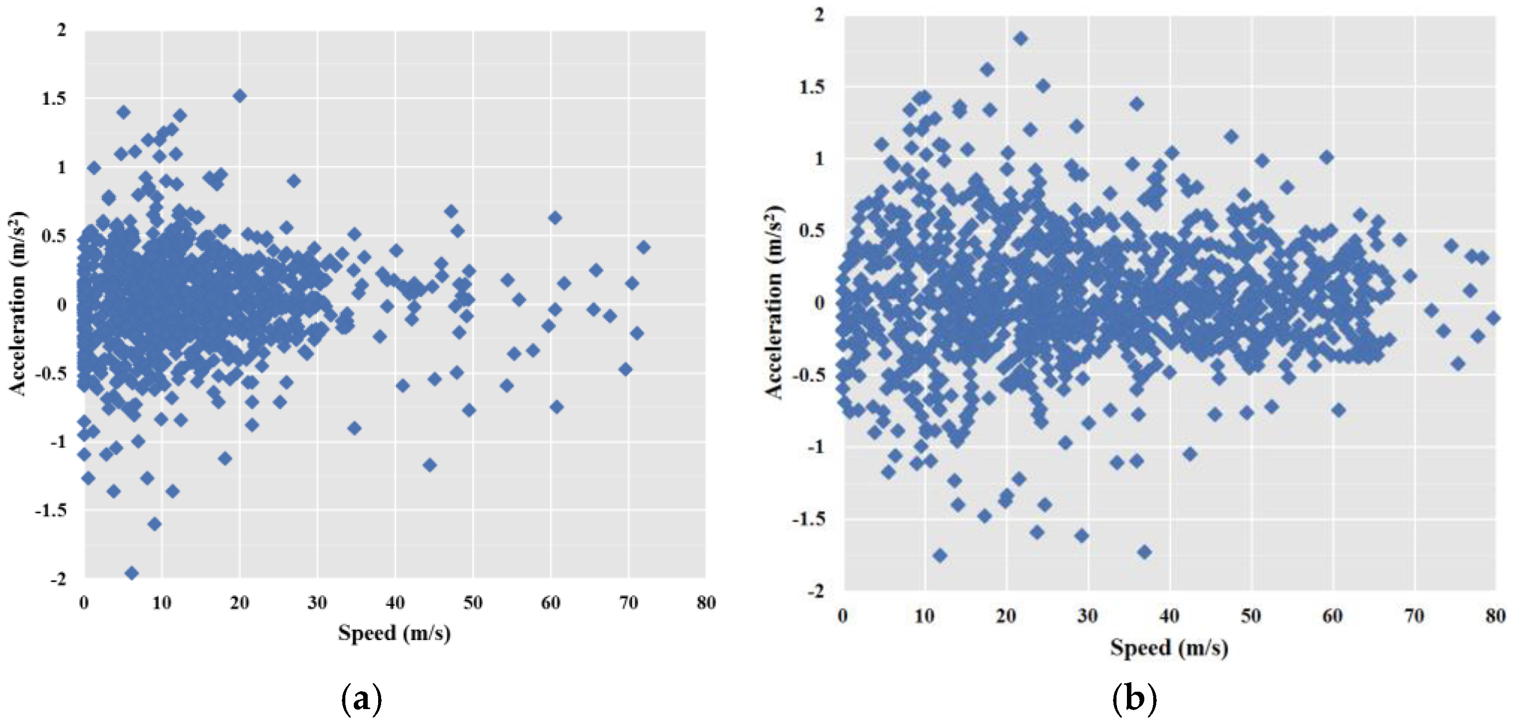
- Distribution of speed acceleration driving condition points
- Localized vehicle driving cycle in Tianjin
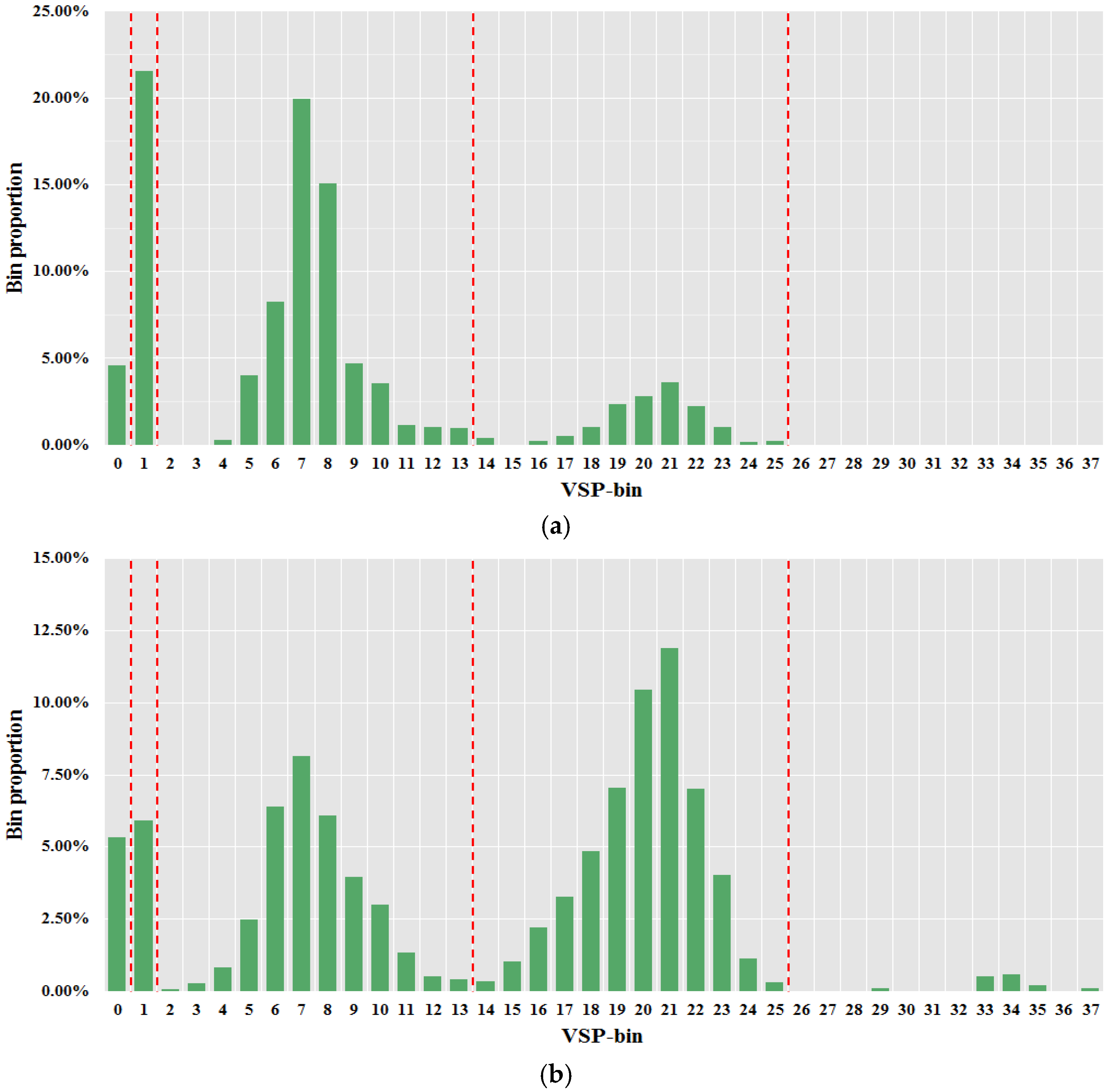
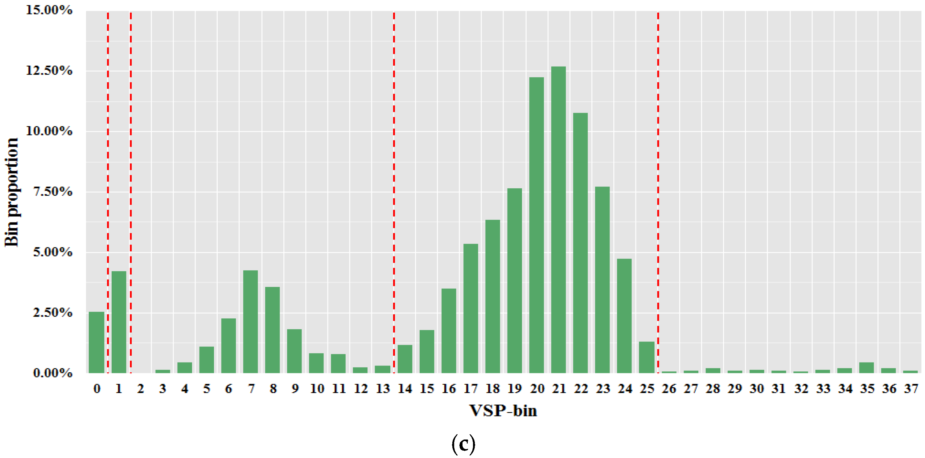
3.1.3. VSP-Bin Frequency Distribution of Driving Conditions
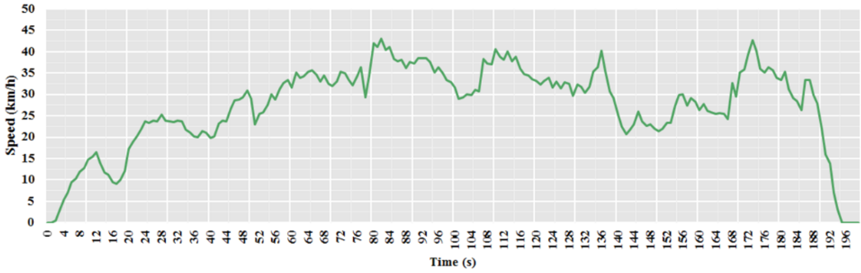
- Driving cycles of different speed intervals
- VSP-bin frequency distributions of different typical driving conditions
- (a)
- The frequency distribution of VSP-bin in different typical vehicle driving cycles was different;
- (b)
- The distribution frequency of different vehicle typical driving cycles was relatively high in bin0 (Deceleration), bin1 (Idling), bin6–bin8 (Low speed), bin19–bin23 (Middle speed);
- (c)
- For the three speed intervals except Deceleration and Idling, the distribution frequency of VSP-bin in the middle of each interval was higher, and the distribution frequency of low VSP-bins and high VSP-bins were less, showing the characteristics of “high in the middle and low at both ends”;
- (d)
- The low speed interval (bin2–bin13) had the highest distribution frequency for low-speed driving cycle, while the middle speed interval (bin14–bin25) had the highest distribution frequency for middle- and high-speed driving cycles. The frequency of the three driving cycles distributed in the high speed interval (bin26–bin37) was very small or even zero.
3.2. Establishment of Vehicle Emission Model
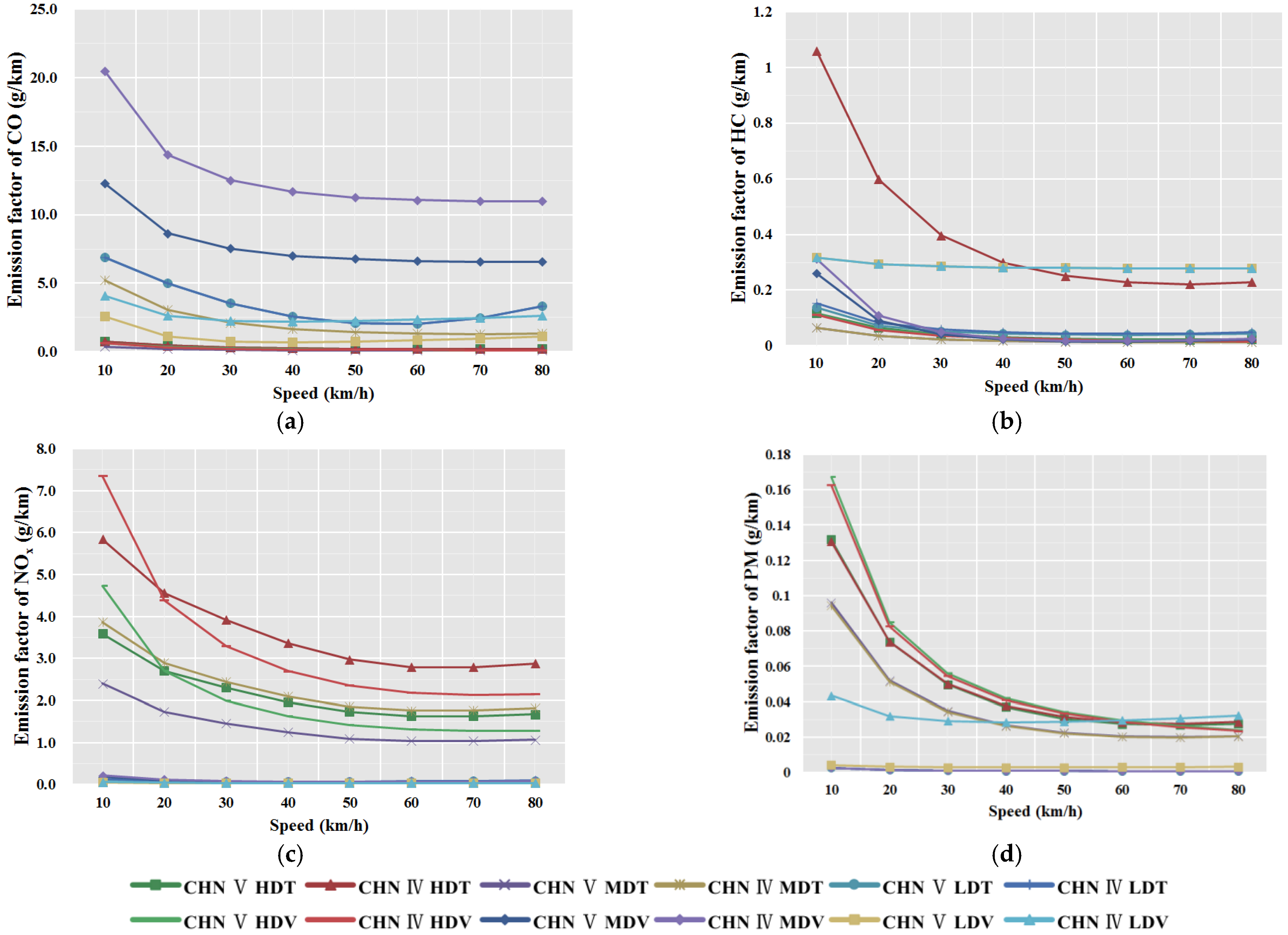
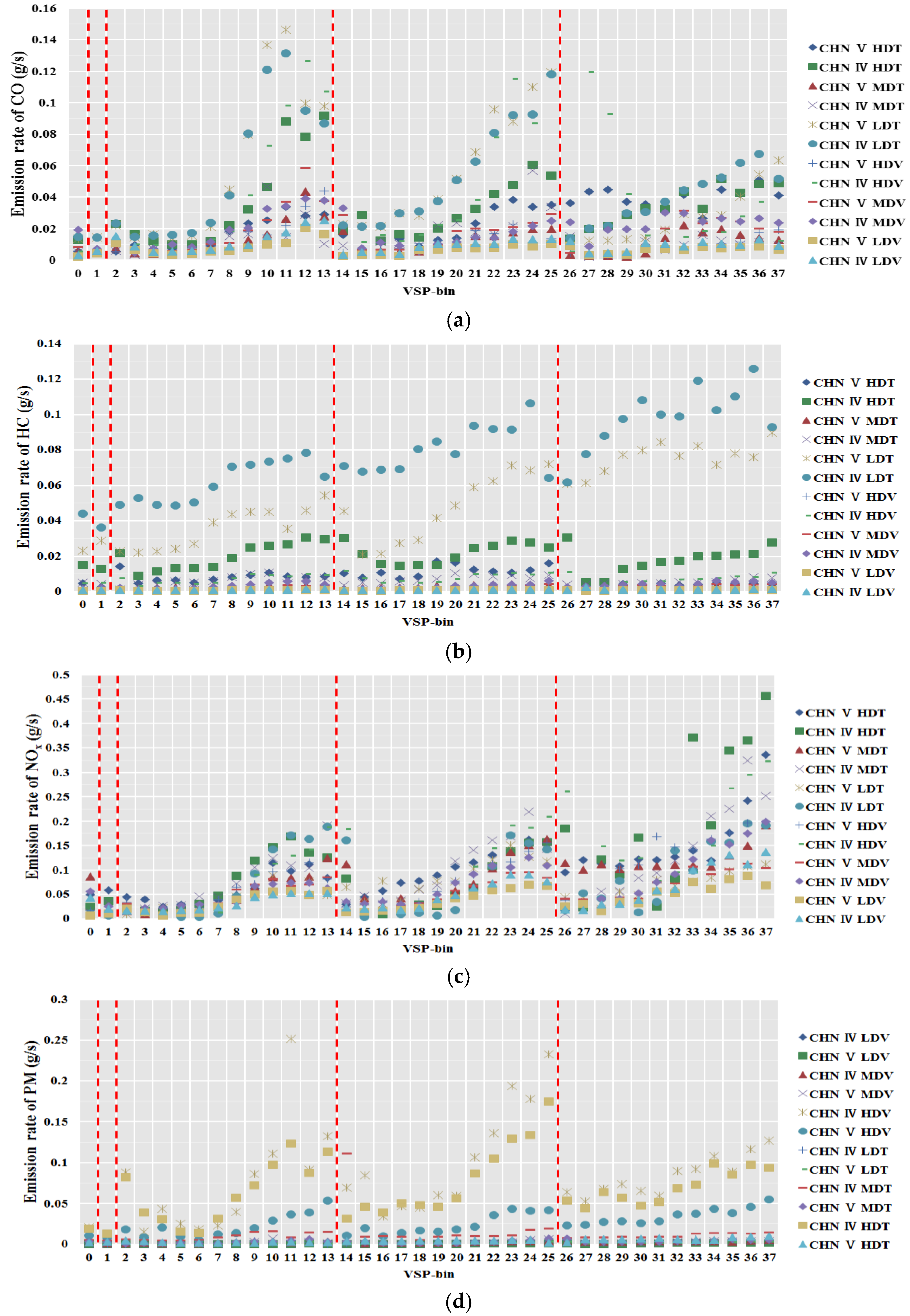
3.2.1. Establishment of Emission Rate Database
- (a)
- The corresponding relationship between emission rate of different types of vehicles and VSP-bins was different;
- (b)
- For the three speed intervals except deceleration and idling, the emission rate of each type of vehicle increased with the increase in VSP-bin;
- (c)
- CHN IV vehicle emission rate was generally higher than the same type CHN V vehicle;
- (d)
- The emission rate of CO and HC of passenger car was generally higher than that of freight car, and the emission rate of NOx and PM of freight was generally higher than that of passenger car.
3.2.2. Calculation of Emission Factors
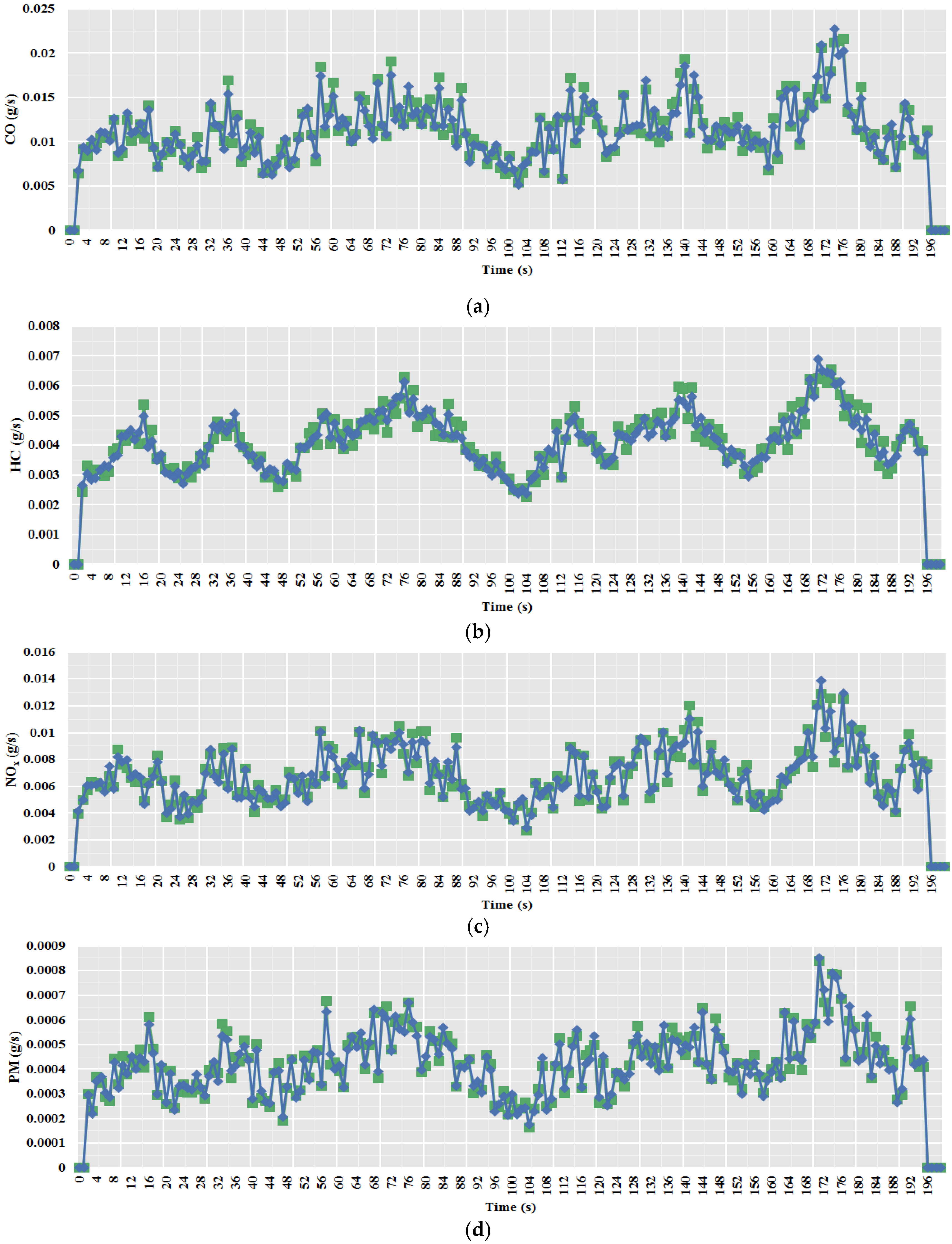
3.2.3. Validation of Emission Model
4. Conclusions
Author Contributions
Funding
Institutional Review Board Statement
Informed Consent Statement
Data Availability Statement
Acknowledgments
Conflicts of Interest
References
- Zhang, Y.; Andre, M.; Liu, Y.; Wu, L.; Jing, B.; Mao, H. Evaluation of low emission zone policy on vehicle emission reduction in Beijing, China. IOP Conf. 2017, 121, 052070. [Google Scholar] [CrossRef] [Green Version]
- Zhang, Y.; André, M.; Liu, Y.; Ren, P.; Yang, Z.; Yuan, Y.; Mao, H. Research on vehicle activity characteristics of typical roads in Tianjin. Environ. Pollut. Control. 2018, 40, 365–372. [Google Scholar]
- Zhang, Y.; Wu, L.; Zou, C.; Jing, B.; Li, X.; Barlow, T.; Kevin, T.; André, M.; Liu, Y.; Ren, P.; et al. Development and application of urban high temporal-spatial resolution vehicle emission inventory model and decision support system. Environ. Model. Assess. 2017, 22, 445–458. [Google Scholar] [CrossRef]
- Gautam, S.; Patra, A.K.; Kumar, P. Status and chemical characteristics of ambient PM2.5 pollutions in China: A review. Environ. Model. Assess. 2019, 21, 1649–1674. [Google Scholar] [CrossRef]
- Gautam, S.; Yadav, A.; Tsai, C.J.; Kumar, P. A review on recent progress in observations, sources, classification and regulations of PM2.5 in Asian environments. Environ. Sci. Pollut. Res. 2016, 23, 21165–21175. [Google Scholar] [CrossRef] [PubMed]
- Ministry of Ecological Environment (MEE). China Vehicle Environmental Management Annual Report (2020); Ministry of Ecological Environment (MEE): Beijing, China, 2020. [Google Scholar]
- Wu, Y.; Wang, R.; Zhou, Y.; Lin, B.; Fu, L.; He, H.; Hao, J. On-road vehicle emission control in Beijing: Past present and future. Environ. Sci. Technol. 2011, 45, 147–153. [Google Scholar] [CrossRef]
- Mahabir, R.S.; Patmore, K.; Liu, H.; Ahluwalia, J.J.; Lanigan, A. Implications of using MOBILE6.2 versus MOVES for transportation air quality assessments. Proc. A Was. Mana. Assoc. Ann. Con. Exh. 2014, 3, 2185–2191. [Google Scholar]
- Lin, C.; Zhou, X.; Wu, D.; Gong, B. Estimation of Emissions at Signalized Intersections Using an Improved MOVES Model with GPS Data. Int. J. Environ. Res. Public Health 2019, 16, 3647. [Google Scholar] [CrossRef] [Green Version]
- Ekström, M.; Sjödin, A.; Andreasson, K. Evaluation of the COPERT III emission model with on-road optical remote sensing measurements. Atmos. Environ. 2004, 38, 6631–6641. [Google Scholar] [CrossRef]
- Smit, R.; Kingston, P. Measuring on-road vehicle emissions with multiple instruments including remote sensing. Atmosphere 2019, 10, 516. [Google Scholar] [CrossRef] [Green Version]
- Mathissen, M.; Grigoratos, T.; Lahde, T.; Vogt, R. Brake wear particle emissions of a passenger car measured on a chassis dynamometer. Atmosphere 2019, 10, 556. [Google Scholar] [CrossRef] [Green Version]
- Qu, L.; Wang, W.; Li, M.; Xu, X.; Jin, T. Dependence of pollutant emission factors and fuel consumption on driving conditions and gasoline vehicle types. Atmos. Pollut. Res. 2020, 12, 137–146. [Google Scholar] [CrossRef]
- Ministry of Ecological Environment (MEE). Technical Guide for the Compilation of Air Pollutant Emission Inventory of Road Vehicles (Trial); Ministry of Ecological Environment (MEE): Beijing, China, 2015. [Google Scholar]
- Raparthi, N.; Debbarma, S.; Phuleria, H.C. Development of real-world emission factors for on-road vehicles from motorway tunnel measurements. Atmos. Environ. 2021, 10, 100113. [Google Scholar] [CrossRef]
- Song, C.; Yan, L.; Sun, S.; Sun, L.; Zhang, Y.; Chao, M. Vehicular volatile organic compounds (VOCs)-NOx-CO emissions in a tunnel study in northern China: Emission factors, profiles, and source apportionment. Atmos. Chem. Phys. 2018, 6, 1–38. [Google Scholar]
- Yang, Z.; Liu, Y.; Wu, L.; Martinet, S.; Zhang, Y.; André, M.; Mao, H. Real-world gaseous emission characteristics of Euro 6b light-duty gasoline- and diesel-fueled vehicles. Transp. Res. Part D Transp. Environ. 2020, 78, 1–11. [Google Scholar] [CrossRef]
- Keogh, D.U.; Darrell, S. Challenges and approaches for developing ultrafine particle emission inventories for motor vehicle and bus fleets. Atmosphere 2011, 2, 36–56. [Google Scholar] [CrossRef] [Green Version]
- Ge, Z.; Zhao, W.; Lyu, L.; Zhu, Z. Fast identification of the failure of heavy-duty diesel particulate filters using a low-cost condensation particle counter based system. Atmosphere 2022, 13, 268. [Google Scholar] [CrossRef]
- Tianjin Municipal Bureau of Statistics (TMBS). Tianjin Statistical Yearbook (2020); Tianjin Municipal Bureau of Statistics (TMBS): Tianjin, China, 2020. [Google Scholar]
- Fomunung, I. Predicting Emissions Rates for the Atlanta on-Road Light-Duty Vehicular Fleet as a Function of Operating Modes, Control Technologies and Engine Characteristics; Georgia Institute of Technology: Atlanta, GA, USA, 2000. [Google Scholar]
- Yang, P.; Liu, Y.; Huang, Y.; Lin, X.; Sha, Z. Effects of traffic states on dynamic emissions of buses based on ES-VSP distribution. Res. Environ. Sci. 2017, 30, 1793–1800. [Google Scholar]
- Ma, C.; Wu, L.; Mao, H.J.; Fang, X.Z.; Yang, L. Transient characterization of automotive exhaust emission from different vehicle types based on on-road measurements. Atmosphere 2020, 11, 64. [Google Scholar] [CrossRef] [Green Version]
- Dong, H.; Xu, Y.; Chen, N. A research on the vehicle emission factors of real world driving cycle in Hangzhou City based on IVE model. Atmos. Environ. 2011, 33, 1034–1038. [Google Scholar]
- Liu, X. A more accurate method using MOVES (Motor Vehicle Emission Simulator) to estimate emission burden for regional-level analysis. J. Air Waste Manag. Assoc. 2015, 65, 837–843. [Google Scholar] [CrossRef] [PubMed]
- Hao, Y.; Deng, S.; Qiu, Z.; Liu, Q.; Gao, C.; Xu, Y. Vehicle emission inventory for Xi’an based on MOVES model. Environ. Pollut. Control. 2017, 39, 227–231. [Google Scholar]
- Frey, H.; Zhang, K.; Rouphail, N.M. Vehicle-specific emissions modeling based upon on-road measurements. Environ. Sci. Technol. 2010, 44, 3594–3600. [Google Scholar] [CrossRef] [PubMed]
- Palacios, J. Understanding and Quantifying Motor Vehicle Emissions with Vehicle Specific Power and TILDAS Remote Sensing; Massachusetts Institute of Technology: Cambridge, MA, USA, 1999. [Google Scholar]
- Li, Z.; Hu, J.; Bao, X.; Pu, Y.; Zhang, G.; Gai, Y. Gaseous pollutant emission of China 3 heavy-duty diesel vehicles under real-world driving conditions. Environ. Sci. Pollut. Res. 2009, 22, 1389–1394. [Google Scholar]


| Deceleration | m/s2) | ||
|---|---|---|---|
| Idling | |||
| VSP (kW/t) | Low Speed | Middle Speed | High Speed |
| ≤−8] | bin2 | bin14 | bin26 |
| (−8,−6] | bin3 | bin15 | bin27 |
| (−6,−4] | bin4 | bin16 | bin28 |
| (−4,−2] | bin5 | bin17 | bin29 |
| (−2,0] | bin6 | bin18 | bin30 |
| (0,2] | bin7 | bin19 | bin31 |
| (2,4] | bin8 | bin20 | bin32 |
| (4,6] | bin9 | bin21 | bin33 |
| (6,8] | bin10 | bin22 | bin34 |
| (8,10] | bin11 | bin23 | bin35 |
| (10,12] | bin12 | bin24 | bin36 |
| >12 | bin13 | bin25 | bin37 |
| No. | Vehicle Driving Characteristic Parameters | Abbreviation |
|---|---|---|
| 1 | Average speed (including idle process), km/h | V1 |
| 2 | Average speed (excluding idle process), km/h | V2 |
| 3 | The average acceleration of all accelerated states, m/s2 | A |
| 4 | The average deceleration of all decelerated states, m/s2 | D |
| 5 | Percentage of idle state time, % | Pi |
| 6 | Percentage of accelerated state time, % | Pa |
| 7 | Percentage of uniform state time, % | Pc |
| 8 | Percentage of decelerated state time, % | Pd |
| 9 | Positive acceleration kinetic energy, m/s2 | PKE |
| 10 | Relative positive acceleration, m/s2 | RPA |
| 11 | The number of times of speed oscillations per 100 m | FDA |
| Emission Standards | CHN Ⅳ | CHN Ⅴ | SUM |
|---|---|---|---|
| Light-duty vehicle (LDV) | 10 | 10 | 20 |
| Middle-duty vehicle (MDV) | 2 | 2 | 4 |
| Heavy-duty vehicle (HDV) | 3 | 3 | 6 |
| Light-duty truck (LDT) | 3 | 3 | 6 |
| Middle-duty truck (MDT) | 4 | 4 | 8 |
| Heavy-duty truck (HDT) | 2 | 2 | 4 |
| SUM | 24 | 24 | 48 |
| Driving Cycles | Driving Cycle in Tianjin | European NEDC | American FTP75 |
|---|---|---|---|
| V1 (km/h) | 27.63 | 33.6 | 34.2 |
| V2 (km/h) | 36.89 | 44.4 | 38.8 |
| A (m/s2) | 0.51 | 0.48 | 0.56 |
| D (m/s2) | −0.51 | −0.68 | −0.67 |
| Pi (%) | 12.98 | 25 | 19 |
| Pa (%) | 36.85 | 27 | 36 |
| Pc (%) | 21.27 | 29 | 16 |
| Pd (%) | 33.18 | 19 | 30 |
| PKE (m/s2) | 0.37 | 0.22 | 0.35 |
| RPA (m/s2) | 0.18 | 0.12 | 0.18 |
| FDA | 1.35 | 0.17 | 0.59 |
| Speed Intervals of VSP-Bins | Low-Speed Driving Cycle | Middle-Speed Driving Cycle | High-Speed Driving Cycle |
|---|---|---|---|
| Deceleration (bin0) | 4.60% | 5.32% | 2.53% |
| Idling (bin1) | 21.58% | 5.93% | 4.22% |
| Low speed (bin2-bin13) | 58.99% | 33.52% | 15.86% |
| Middle speed (bin14-bin25) | 14.84% | 53.64% | 75.35% |
| High speed (bin26-bin37) | 0.00% | 1.51% | 2.03% |
| CO | HC | NOx | PM | |||||||||
|---|---|---|---|---|---|---|---|---|---|---|---|---|
| Vehicles Types | Simulation | NEDC | FTP75 | Simulation | NEDC | FTP75 | Simulation | NEDC | FTP75 | Simulation | NEDC | FTP75 |
| CHN Ⅳ LDV | 0.681 | 0.496 | 0.545 | 0.077 | 0.061 | 0.057 | 0.031 | 0.021 | 0.025 | 0.003 | 0.002 | 0.002 |
| CHN Ⅴ LDV | 0.455 | 0.276 | 0.379 | 0.059 | 0.038 | 0.046 | 0.017 | 0.013 | 0.014 | 0.003 | 0.002 | 0.002 |
| CHN Ⅳ MDV | 2.060 | 1.351 | 1.555 | 0.105 | 0.070 | 0.080 | 0.197 | 0.128 | 0.167 | 0.007 | 0.005 | 0.006 |
| CHN Ⅴ MDV | 1.990 | 1.197 | 1.537 | 0.102 | 0.069 | 0.083 | 0.153 | 0.104 | 0.123 | 0.007 | 0.005 | 0.006 |
| CHN Ⅳ HDV | 2.250 | 1.776 | 1.799 | 0.106 | 0.083 | 0.082 | 5.040 | 3.960 | 3.865 | 0.277 | 0.176 | 0.212 |
| CHN Ⅴ HDV | 1.660 | 1.213 | 1.287 | 0.084 | 0.056 | 0.067 | 4.000 | 2.535 | 3.393 | 0.140 | 0.109 | 0.110 |
| CHN Ⅳ LDT | 2.400 | 1.804 | 1.819 | 0.169 | 0.103 | 0.123 | 2.240 | 1.728 | 1.734 | 0.007 | 0.006 | 0.005 |
| CHN Ⅴ LDT | 2.350 | 1.418 | 1.947 | 0.165 | 0.103 | 0.121 | 2.170 | 1.501 | 1.740 | 0.007 | 0.004 | 0.005 |
| CHN Ⅳ MDT | 1.720 | 1.302 | 1.340 | 0.105 | 0.076 | 0.081 | 4.310 | 3.203 | 3.652 | 0.107 | 0.076 | 0.084 |
| CHN Ⅴ MDT | 1.610 | 1.253 | 1.324 | 0.105 | 0.079 | 0.082 | 3.620 | 2.776 | 2.983 | 0.021 | 0.016 | 0.018 |
| CHN Ⅳ HDT | 2.210 | 1.672 | 1.874 | 0.134 | 0.097 | 0.098 | 5.380 | 4.217 | 4.387 | 0.149 | 0.112 | 0.122 |
| CHN Ⅴ HDT | 2.170 | 1.472 | 1.818 | 0.126 | 0.098 | 0.099 | 4.620 | 3.463 | 3.887 | 0.030 | 0.021 | 0.024 |
Publisher’s Note: MDPI stays neutral with regard to jurisdictional claims in published maps and institutional affiliations. |
© 2022 by the authors. Licensee MDPI, Basel, Switzerland. This article is an open access article distributed under the terms and conditions of the Creative Commons Attribution (CC BY) license (https://creativecommons.org/licenses/by/4.0/).
Share and Cite
Zhang, Y.; Zhou, R.; Peng, S.; Mao, H.; Yang, Z.; Andre, M.; Zhang, X. Development of Vehicle Emission Model Based on Real-Road Test and Driving Conditions in Tianjin, China. Atmosphere 2022, 13, 595. https://doi.org/10.3390/atmos13040595
Zhang Y, Zhou R, Peng S, Mao H, Yang Z, Andre M, Zhang X. Development of Vehicle Emission Model Based on Real-Road Test and Driving Conditions in Tianjin, China. Atmosphere. 2022; 13(4):595. https://doi.org/10.3390/atmos13040595
Chicago/Turabian StyleZhang, Yi, Ran Zhou, Shitao Peng, Hongjun Mao, Zhiwen Yang, Michel Andre, and Xin Zhang. 2022. "Development of Vehicle Emission Model Based on Real-Road Test and Driving Conditions in Tianjin, China" Atmosphere 13, no. 4: 595. https://doi.org/10.3390/atmos13040595
APA StyleZhang, Y., Zhou, R., Peng, S., Mao, H., Yang, Z., Andre, M., & Zhang, X. (2022). Development of Vehicle Emission Model Based on Real-Road Test and Driving Conditions in Tianjin, China. Atmosphere, 13(4), 595. https://doi.org/10.3390/atmos13040595