Article

Simulated Methane Emission Detection Capabilities of Continuous Monitoring Networks in an Oil and Gas Production Region

Center for Energy and Environmental Resources, University of Texas at Austin, Austin, TX 78758, USA
*
Author to whom correspondence should be addressed.
Atmosphere 2022, 13(4), 510; https://doi.org/10.3390/atmos13040510
Submission received: 17 February 2022 / Revised: 18 March 2022 / Accepted: 21 March 2022 / Published: 23 March 2022

Abstract

:
Simulations of the atmospheric dispersion of methane emissions were created for a region containing 26 oil and gas production sites in the Permian Basin in Texas. Virtual methane sensors were placed at 24 of the 26 sites, with at most 1 sensor per site. Continuous and intermittent emissions from each of the 26 oil and gas production sites, over 4 week-long meteorological episodes, representative of winter, spring, summer, and fall meteorology, were simulated. The trade-offs between numbers of sensors and precision of sensors required to reliably detect methane emissions of 1 to 10 kg/h were characterized. A total of 15 sensors, able to detect concentration enhancements of 1 ppm, were capable of identifying emissions at all 26 sites in all 4 week-long meteorological episodes, if emissions were continuous at a rate of 10 kg/h. More sensors or sensors with lower detection thresholds were required if emissions were intermittent or if emission rates were lower. The sensitivity of the required number of sensors to site densities in the region, emission dispersion calculation approaches, meteorological conditions, intermittency of the emissions, and emission rates, were examined. The results consistently indicated that, for the conditions in the Permian Basin, a fixed monitoring network with approximately one continuous monitor per site is likely to be capable of consistently detecting site-level methane emissions in the range of 5–10 kg/h.

1. Introduction

Methane emissions from oil and gas production sites are detected and quantified in a variety of ways [1]. Some sensing approaches are short-duration measurements of methane concentrations using equipment deployed on foot, on drones, on ground vehicles, on aircraft, or on satellites. These short-term measurements, which employ a wide variety of detection technologies, capture instantaneous snapshots of methane concentrations, which can be used to estimate emission rates. Since many emission sources in upstream oil and gas operations are intermittent, short-term measurements may not detect all emissions from a site or may observe an intermittent emission that is then interpreted as persistent. In addition, since most short-term measurements are deployed on a monthly, quarterly, semi-annual, or annual basis, emissions that develop between measurements could persist undetected until the next scheduled measurement. If these emission rates are large, total emissions could be dominated by sources that develop between scheduled measurements. These limitations of periodic, short-duration measurements have driven interest, including regulatory initiatives [2,3], in continuous monitoring of emissions, using networks of sensors. The primary advantage of a continuous monitoring network is that it may be able to detect methane emissions much more quickly than detection methods based on short sampling times that are periodically repeated. The disadvantage of such networks is the cost of deploying the large numbers of sensors which would be required to enable a network to reliably and quickly detect unintended emissions.
This work will examine how many sensors, with what precision, would be required in a prototypical continuous monitoring network for methane emissions. The effectiveness of a prototypical network for detecting methane emissions in the Permian Basin oil and gas production region in West Texas will be assessed. The Permian Basin is one of the largest oil and gas production regions in the world, with 2019 gas production, in just the portion of the Permian Basin in the State of Texas, of approximately 11.8 billion cubic feet/day (~4 trillion cubic feet/year, approximately 10% of total US production) and oil production of approximately 3 million barrels per day (approximately a quarter of total US production) [4]. Recent assessments of methane emissions from the Permian Basin, based on TROPOMI satellite data, have estimated the methane emission rate as 2.9 Tg per year, a rate equivalent to approximately 3.7% of the volume of gas produced [5]. In addition to having methane emissions and methane emission intensities (methane emitted/natural gas produced) that are among the largest in the United States, the Permian Basin has simple topography and persistent winds, making the basin an ideal location for continuous monitoring using networks of fixed sensors.
The multiple operators and close proximity of sites in the Permian Basin also enhance the advantages of a shared network of sensors. As will be demonstrated in this work, because of the density and proximity of sites (>3 site/km2 in the region examined), most unintended emissions could, in principle, be detected without having multiple sensors surrounding every site. Compared to isolated sites requiring sensors located at multiple cardinal directions (e.g., sensors north, south, east, and west of each site), sensors in the Permian Basin could be located at nearby sites (e.g., sites to the north, south, east, and west of a central site) to replace some of the information that would be provided by multiple sensors for isolated sites.
To evaluate the ability of a fixed network of methane sensors to detect emissions in the Permian Basin, a domain consisting of 26 oil and gas production sites and a flare site, near Midland Texas, was chosen. Four meteorology episodes, each one week in duration, were chosen as representative of seasonal variability in wind speed and direction. The dispersion of simulated emissions from each of the 26 oil and gas production sites was modeled for each week-long episode. The concentration enhancements due to emissions, from each source location, that would be detected at monitoring sites located near each source location were estimated. Analyses were performed for individual and collective weeks of meteorology, each representative of a season. Details of the analyses are described in the Methodology Section and in the Supplementary Materials. The overall goal of the analysis, however, is to characterize trade-offs between numbers of sensors and the precision of sensors required in order to reliably detect emissions, of various magnitudes, using a fixed monitoring network in an oil and gas production region.
This analysis represents a best-case scenario for fixed methane monitoring networks. The region chosen for modeling has site densities of >3 per square kilometer. Winds are generally strong and persistent. Emissions, some continuous and some intermittent, are assumed to persist for the week-long periods modeled. Dispersion models are assumed to accurately characterize the relationship between emission rates and methane concentrations at sensor sites. Sensors are assumed to accurately track simulated concentrations, and data analytics are assumed to be available such that concentration enhancements above the sensor’s precision would reliably be attributed to an emission source. The response of the number of sensors required in the network to the conditions used in the simulations is considered in sensitivity analyses, however even the most idealized analysis characterizes important and basic trade-offs in the design of continuous monitoring networks for methane. This work demonstrates an approach to the design of low-cost methane sensing networks that minimizes the number of sensors required while meeting objectives of emission detection. The results show that, in principle, a relatively small number of sensors is capable of detecting site-level methane emissions of 5–10 kg/h in the Permian Basin. In the few production regions that have had large, multi-scale campaigns to measure methane emissions, this level of emissions has been shown to represent a significant fraction of total emissions. For example, in the Barnett Shale of North Central Texas, the 10% of sites with emissions above 5 kg/h were estimated to account for approximately a third of all emissions, and a much larger fraction of emissions attributed to abnormal operations [6]. In addition, the framework described here for the design of continuous monitoring of methane emissions could be applied to continuous monitoring of other air pollutants, using low-cost sensors. The analyses in this manuscript represent a proof of concept for the design of fixed monitoring networks for methane or other air pollutants. Sensor deployment, testing, and emission detection studies are ongoing, but are beyond the scope of this paper.

2. Materials and Methods
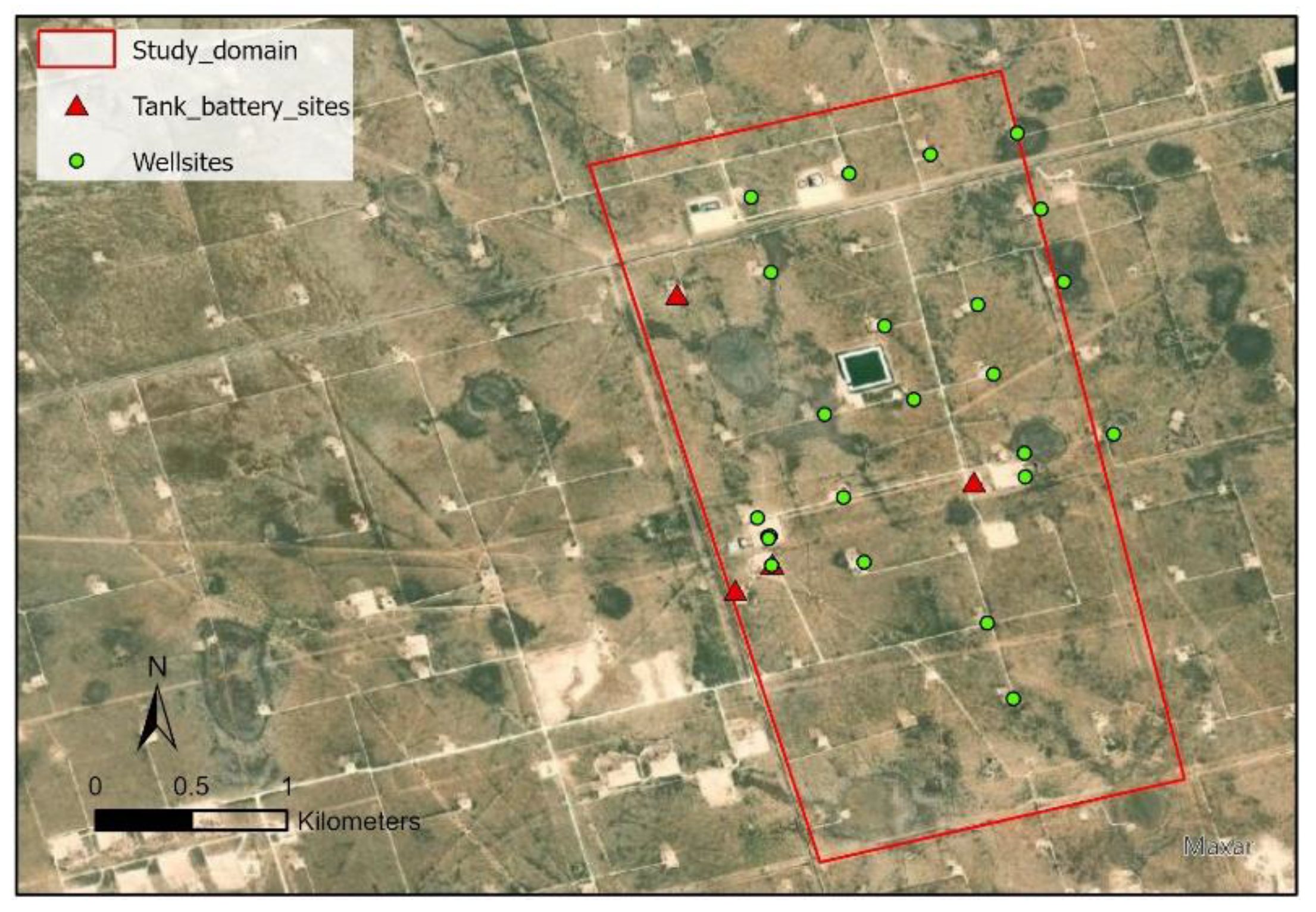
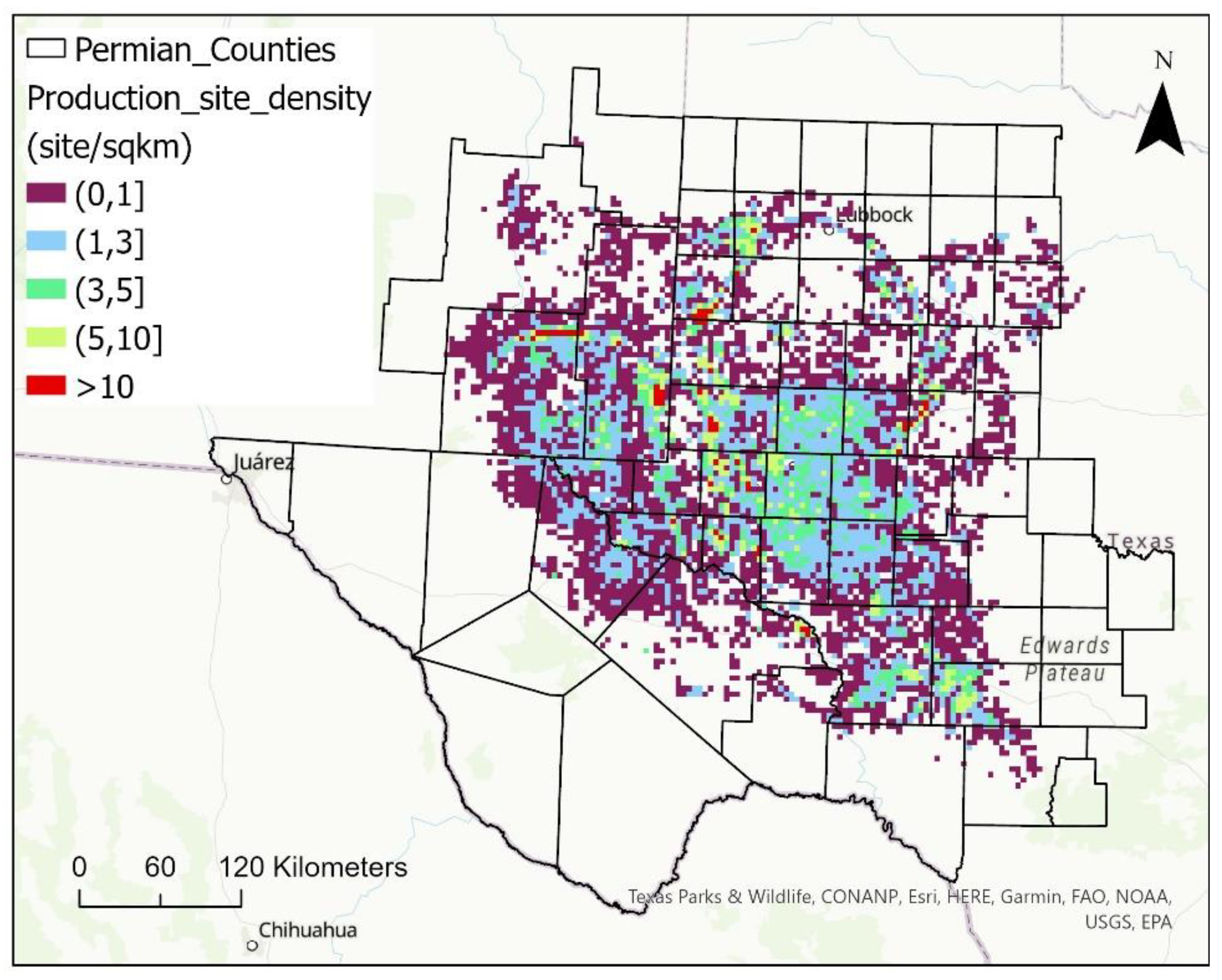
2.1. Modeled Domain

A 1.9 by 3.7 km rectangular region in Midland County in Texas was chosen as the modeling domain. The region contains well sites, centralized facilities that collect production from multiple wells (tank battery sites), and a flare site (assumed idle). A satellite image of the region is shown in Figure 1, with wells and tank battery sites identified as emission sites. Three operators have a total of twenty-four wells and four tank battery sites in the domain. Wells appearing on the same well pad are clustered as a well site. The 24 wells in the domain are clustered into 22 well sites. This specific region was chosen since the clustering and relative positioning of the wells and tank batteries are representative of the asset designs used by multiple operators in the Permian Basin.

2.2. Emission Detection

Available methane sensors that might be deployed in a fixed monitoring network vary in their precision [7]. The precision of the sensor influences the ability of the sensor to detect emissions. Therefore, a variety of emission detection thresholds were considered. In this work, an emission was counted as detectable if during a one-week period, any sensor location in the network is predicted to observe a concentration enhancement greater than either 200, 500, or 1000 ppb (0.2, 0.5, or 1 ppm) for at least 1 minute. These thresholds for detection were based on the variability in background concentrations of methane observed in the region. A recent multi-month field study [8], evaluating low-cost methane sensors, found that daily minimum concentrations of methane (representative of background concentrations) in the region were 1.96 ppm, with a standard deviation of 0.05 ppm. An emission was assumed to be undetectable if no sensors in the network observe a concentration enhancement greater than these thresholds over a one-week period. This work examines the number of sensors and detection thresholds required to detect emissions from all sources in the region if methane is emitted at a rate of 10 kg/h. The analysis was repeated for emission rates of 5 and 1 kg/h.

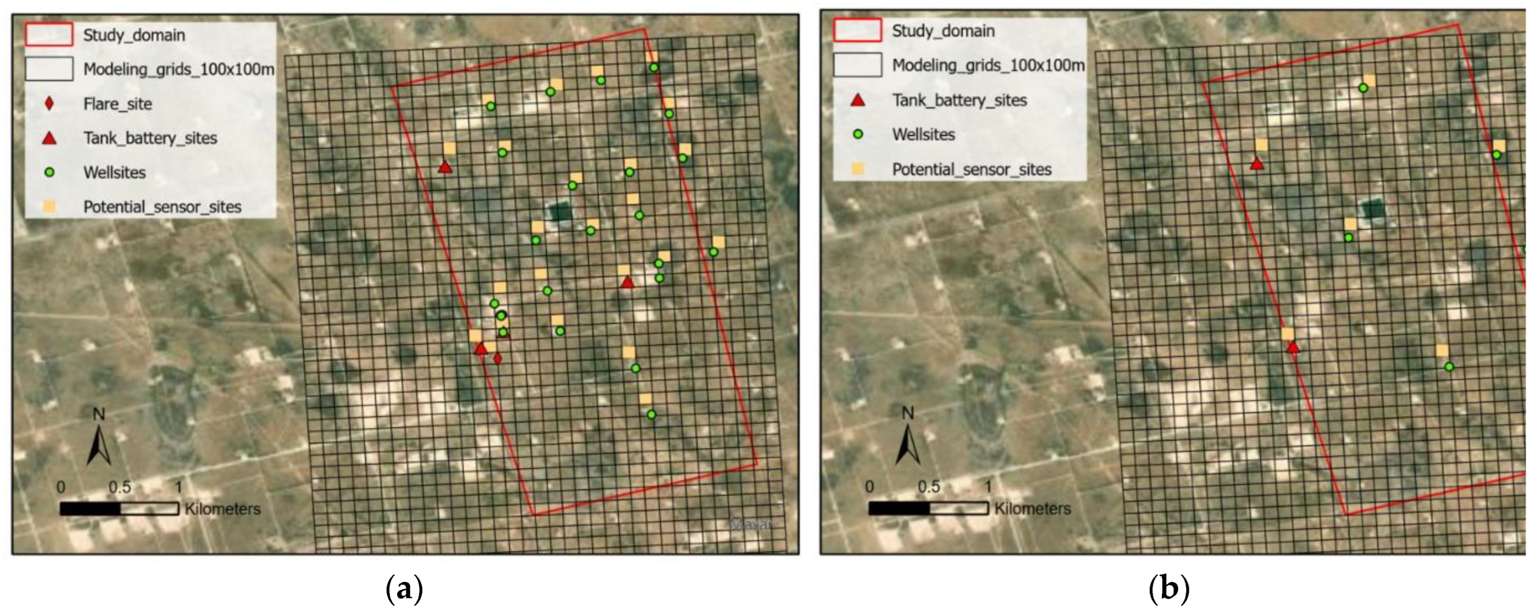
2.3. Emissions and Sensor Placement

Emissions from each of the 22 well sites and the 4 tank battery sites in the domain were modeled. Emissions were not modeled for a flare site in the region. The flare was assumed to be idle at most times, and if it were to be combusting gas, unintended emissions would be due to unlit operation or very low combustion efficiencies. Unlit or low combustion efficiency emissions would lead to ambient concentrations of methane that would be readily detectable by the sensor network. The emissions from each of the well and tank battery sites were modeled separately (different simulations for each location). Emissions in each simulation were continuous at flow rates of 10, 5, and 1 kg/h, or were intermittent emissions at the same instantaneous flow rate. The intermittent emissions were assumed to occur for 1 min of every hour (e.g., minute 30 of hour 1, minute 30 of hour 2, and minute 30 of all subsequent hours), and when the emissions were occurring, they were assumed to emit at an instantaneous rate equal to the continuous emissions (10, 5, and 1 kg/h). Emissions were assumed to be released from the center of each well site, or tank battery site. Continuous releases from both well sites and tank battery sites and intermittent releases from well sites were assumed to occur at a height of 0.2 m, consistent with emissions associated with leaks from ground-level equipment and piping. Intermittent releases from tank battery sites were assumed to occur at a height of 5.5 m, representative of the height of tanks which have intermittent emissions due to the volatilization and release of methane discharged periodically to the tanks from high-pressure separators. The domain was gridded into 100 by 100 m cells and virtual sensors were placed in the center of the grid cell immediately to the north of each site to take advantage of prevailing southerly wind directions. If another emission site was located in the grid cell immediately to the north of a site, no sensor was placed in the cell. This led to a total of 24 sensor locations, as shown in Figure 2a. A modeling domain with reduced site density (~1 site/km2) was also investigated to assess the importance of the site density. Seven emission sites out of the twenty-six sites in the base case were selected, with all sites separated by ~1 km, as shown in Figure 2b. Sensors were placed in the gird cell immediately to the north of the selected sites.

2.4. Meteorological Episode Selection

Four time periods of one-week duration, from four calendar quarters, were identified to be representative of meteorological conditions during 2019. The year was first divided into four quarters, followed by an evaluation of wind speeds and wind directions observed in each seven-day period within the quarter against the variability seen in the entire quarter. The weeks that captured a reasonable representation of the range and frequency of wind speeds and wind directions observed during each of those quarters were selected as representative weeks (Figure S1). The dataset employed for this selection was obtained from one of the ground-based monitoring stations in the Midland-Odessa area (Continuous Ambient Monitoring Station, CAMS 47, Chennai, India), operated by the Texas Commission on Environmental Quality [9]. Temperature, surface pressure, dew point temperature, and precipitation were compared to observations at the National Weather Service (NWS) Station at Midland International Airport. As shown in Supplementary Figures S1 and S2, the week-long periods were found to be representative of the annual variability in meteorology.

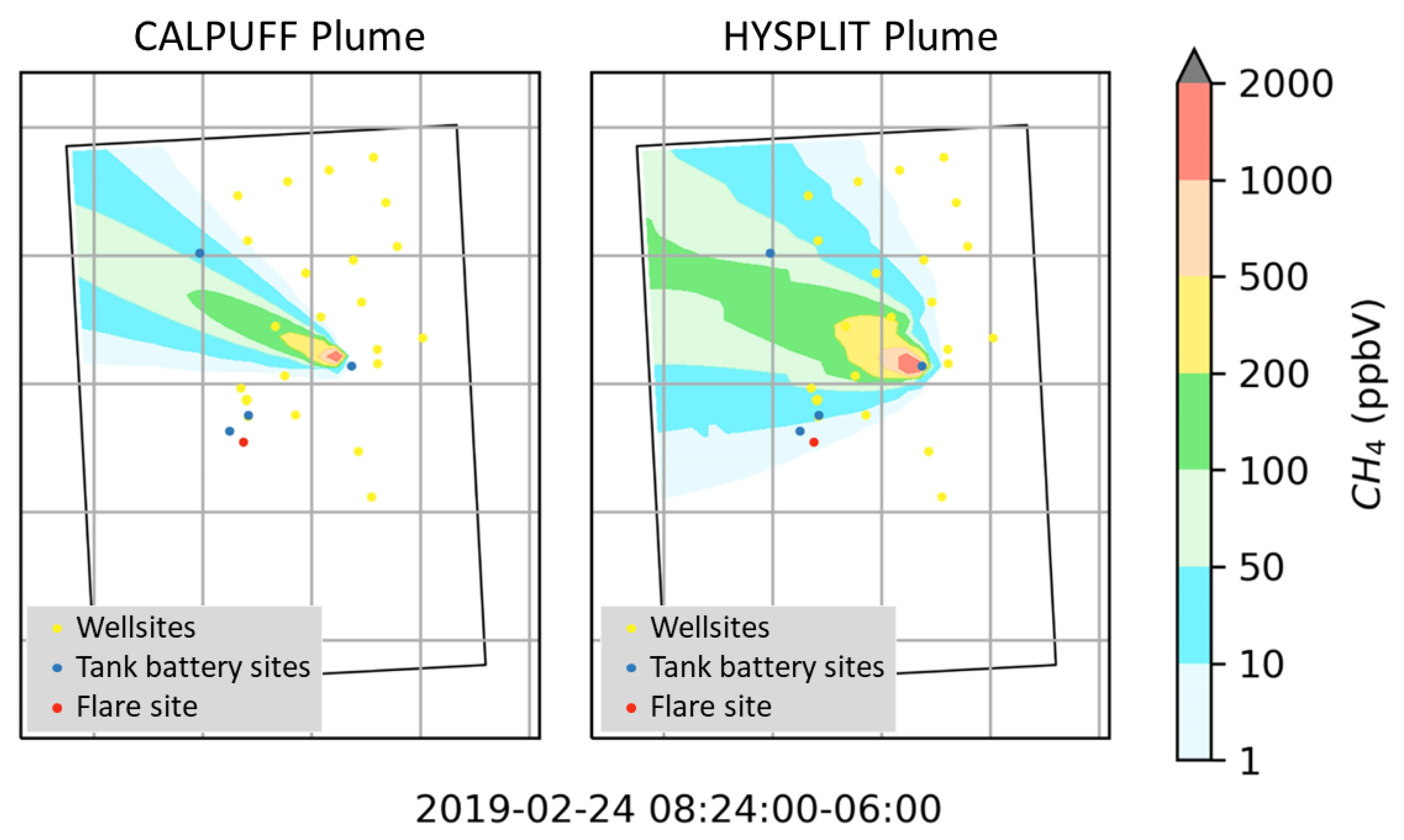
2.5. Dispersion Modeling

To predict concentrations of methane in the modeling domain from each of the emission sources, atmospheric dispersion modeling was utilized. The atmospheric dispersion models use the emissions, together with a representation of 3D meteorological conditions and geophysical and land surface characteristics, to predict downwind concentrations throughout the modeling domain. While the geophysical and surface characteristics are assumed to remain constant, the meteorological conditions can vary considerably depending on the time of day and the time of year. Two dispersion models were used, HYSPLIT (Hybrid Single-Particle Lagrangian Integrated Trajectory, v5.0.0) and CALPUFF (v7.2.1_L150618). The HYSPLIT Model, developed by the National Oceanic and Atmospheric Administration, is one of the most extensively used atmospheric dispersion models [10]. The model calculation method is a hybrid between Lagrangian and Eulerian approaches. It calculates the dispersion of a pollutant by assuming either puff mode or particle mode, or both. For this work, HYSPLIT was used in puff mode. CALPUFF, on the other hand, is a non-steady state, Lagrangian puff modeling system (Exponent, 2014) [11]. The three-dimensional meteorological fields used to drive these models are derived from the output of the North American Mesoscale (NAM) Model Analysis. NAM is a weather model run by the National Centers for Environmental Prediction (NCEP) for producing weather forecasts (out to 84 h) every 6 hours at 0, 6, 12, and 18 UTC (Coordinated Universal Time) [12]. The NAM dataset used in this work is a blend of 4-time daily analyses of observations (at 0, 6, 12, and 18 h) with 3-hour forecasts at 3, 9, 18, and 21 h. It has a spatial resolution of 12 km and a temporal resolution of 3 h. For evaluating this dataset, the observations of wind speed and wind directions at the nearest grid cell were extracted and compared to the observations at the monitoring site maintained by the Texas Commission on Environmental Quality (TCEQ) for the four representative meteorological weeks [9]. The NAM Analysis represented observations with high fidelity. The primary analyses presented in this work will use the CALPUFF dispersion modeling driven by NAM meteorological data. Sensitivity analyses will examine the effect of the choice of dispersion model. The spatial scale of air dispersion modeling for the simulated domain is approximately 7 km2. At this spatial scale and typical near-surface wind speeds in Midland-Odessa (5–30 km/h), emission plumes from oil and gas sources would be transported across the entire grid domain within a few hours, even during periods of very light wind speeds. Therefore, a time resolution of one minute was chosen for the meteorological modeling.

3. Results

3.1. Base Case

Table 1 reports the number of sensors required to detect emissions from each of the 26 emissions sites in each of the 4 weeks of meteorology (104 total detections). Alternative representation of the results are shown in the Supplementary Figure S3. Simulations were performed for each of the individual sites to determine which sensors, at which times, would detect emissions. Due to the unique orientation of each sensor location to each potential source, the detections of emissions from different sites by a single sensor generally do not interfere with each other. A sensor will detect a site to its south only when the winds are from the south, and this detection will not interfere with the ability of the same sensor, at a different time, to detect an emission from a source that is to the east.
Using this approach, at an emission rate of 10 kg/h per site, a total of 15 sensors are required to detect all continuous emission sources if a detection is defined as at least one concentration enhancement of 1000 ppb, due to continuous emissions from a single site, during each of the 4 week-long meteorological episodes. If the detection threshold is lowered to 500 or 200 ppb, the number of required sensors to detect all continuous emissions is reduced to 7 and 4, respectively. A larger number of sensors or more precise sensors are required if emissions are intermittent. For emissions that occur at a rate of 10 kg/h, but only persist for one minute during each hour, the number of sensors required to detect all emission sources with sensor detection thresholds of 500 and 200 ppb is 15 and 8, respectively. If the detection threshold is 1000 ppb, even if sensors are placed at all 24 possible locations, not all emission sources can be detected within a 1-week period. In this scenario with intermittent emissions and a detection threshold of 1000 ppb, 98 of the 104 possible detections (26 sources in each of 4 weeks) are made.
Similar analyses are reported in Table 1 for emission rates of 5 and 1 kg/h. As emission rates are reduced, either more sensors are required, or better sensor sensitivity is required. Nevertheless, a network of approximately 1 sensor per site, with a sensor detection threshold as high as 1000 ppb, is able to detect a very high fraction of emissions from sites with 5–10 kg/h emission rates. Similar results are obtained using the HYSPLIT dispersion model with the NAM meteorological dataset, as documented in Supplementary Table S1.

3.2. Sensitivity Analyses

Analyses were conducted to assess the importance of site density and meteorology on the required number of sensors. Site density was reduced from 26 sites to 7 sites in the same modeling domain, with all sites approximately 1 km apart from each other, as shown in Figure 2b. The same analyses were performed, and results are shown in Table 2 (alternative representation of the results are shown in the Supplementary Figure S4). The results again indicate that a network of approximately 1 sensor per site is able to detect a very high fraction of emissions from sites with 5–10 kg/h emission rates.
The importance of meteorology was assessed by examining the number of sensors required in each of the one-week periods that were chosen to represent seasonal meteorology. Wind speeds and wind directions vary significantly from season to season in the region, as shown in the Supplementary Figure S2. During summer months, wind directions are consistently from the southwest to the southeast. In contrast, winter wind directions are highly variable. This makes detection during summer months more challenging than detection during winter months. Numbers of sensors required for each season, for both the base case analyses and the reduced site density analyses, are presented in Table 3 and Table 4 (alternative representation of the results are shown in the Supplementary Figures S5 and S6). While the number of sensors required in winter months is lower than in summer months, even with the more challenging meteorology of the summer, networks of approximately 1 sensor per site are able to detect a very high fraction of emissions from sites with 5–10 kg/h emission rates.

4. Discussion

As shown in Table 1 and Table 2, for both high (>3 site/km2) and low site density (~1 site/km2) scenarios, a methane monitoring network with approximately 1 sensor per site is able to detect a large fraction of emissions from sites with 5–10 kg/h emission rates. Site densities in this range are common in the Permian Basin. Figure 3 shows production site densities in the Permian Basin in November 2021 [13]. Production sites in the Permian Basin were aggregated into 4 × 4 km2 grid cells, and the site density in each grid cell was calculated and mapped. For grid cells containing at least one production site, 58% had site densities less than 1 site/km2, 28% had site densities between 1 and 3 site/km2, and 8% had site densities between 3 and 5 site/km2. Only 1% of the grid cells had site densities over 10 site/km2. While grid cells with <1 site/km2 represent more than half of the total grid cells with production reported, cells with >1 site/km2 account for 85% of the production in the Permian Basin. Therefore, the analyses represent a proof of concept applicable to a large fraction of the production in the Permian Basin.
As shown in Table 3 and Table 4, the effectiveness of detections was affected by meteorology, which varies significantly from season to season in the region. As shown in the Supplementary Figure S2, during spring and summer months (April to September), winds are primarily from the southwest to the southeast. During these seasons, individual sensors are only able to detect emissions from southerly directions. In contrast, during winter months (October to March), winds are variable in direction, allowing sensors to detect emissions from sources in multiple directions. Therefore, compared to summer months, winter months require less sensors in the network to detect all the emissions in the region. However, even during the summer months, a network with approximately one sensor per site is still able to detect most of the sources with emission rates between 5 and 10 kg/h.
Two different dispersion models were used in this work to evaluate sensor placements. Although the counts of sensors required to detect all emission sources vary with the use of different dispersion models, the conclusion that approximately one continuous monitor per site is able to detect a large fraction of emissions in the range of 5–10 kg/h is valid with either dispersion model applied. Figure 4 shows a comparison of the plumes predicted by the two models at a minute instance during the simulation week in winter, due to a continuous emission source with an emission rate of 25 kg/h at the tank battery site in the middle of the study domain, with the same meteorological dataset. Predictions of vertical and horizontal plume width, and other parameters, vary between the dispersion models. The HYSPLIT model led to more grid cells and sensor locations with concentration enhancements above the detection thresholds. For a single emission source, with HYSPLIT simulations, more sensor locations would be able to consistently detect the emissions. Therefore, analyses conducted with the HYSPLIT dispersion model indicated that slightly fewer sensors are required to be able to consistently detect emissions in the range of 5–10 kg/h, compared to the analyses with the CALPUFF Model (results are shown in Supplementary Table S1). Many different combinations of parameters, used as input to dispersion models, could lead to the slightly different numbers of sensors predicted by the two dispersion models. Overall, however, the analyses consistently indicate that, for the conditions in the Permian Basin, a fixed monitoring network with approximately one continuous monitor per site is likely to be capable of consistently detecting site-level methane emissions in the range of 5–10 kg/h.

5. Conclusions

This paper characterized trade-offs between numbers of sensors and the precision of sensors required to reliably detect methane emissions, ranging from 1 to 10 kg/h, using a fixed continuous methane monitoring network, based in a representative oil and gas production region in the Permian Basin. It demonstrates an approach to the design of methane sensing networks that minimizes the number of sensors required while meeting objectives of emission detection. The number of sensors required to detect continuous and intermittent emissions with various emission rates was examined with two representative site densities, under four meteorological conditions representing four seasons, and with two dispersion models. The results show that although the number of sensors required to detect the emissions varies from case to case, networks with approximately one continuous monitoring sensor per site are capable of detecting site-level methane emissions of 5–10 kg/h in the Permian Basin.

Supplementary Materials

The following Supplementary Materials can be downloaded at: https://www.mdpi.com/article/10.3390/atmos13040510/s1: Figure S1: Wind rose diagrams, showing wind speed frequency data, by wind direction for the four representative weeks and for observational annual average data. Figure S2: Wind roses for each quarter (left) and representative week (right) for quarters 1 (a), 2 (b), 3 (c), and 4 (d). Figure S3: Alternative representation of the results in Table 1. Figure S4: Alternative representation of the results in Table 2. Figure S5: Alternative representation of the results in Table 3. Figure S6: Alternative representation of the results in Table 4. Table S1: Sensors required to detect continuous emissions from each of the 26 emissions sites, in each of the four weeks of meteorology evaluated in this work (104 total detections), using multiple dispersion models.

Author Contributions

Conceptualization, D.T.A.; methodology, all authors; software, Q.C., M.M., G.M. and Y.K.; validation, Q.C., M.M. and Y.K.; formal analysis, Q.C. and M.M.; investigation, Q.C., M.M., G.M. and Y.K.; resources, D.T.A.; data curation, Q.C., M.M. and Y.K.; writing—original draft preparation, Q.C., M.M., G.M. and D.T.A.; writing—review and editing, Q.C. and D.T.A.; visualization, Q.C.; supervision, D.T.A. and E.M.-B.; project administration, D.T.A. and E.M.-B.; funding acquisition, D.T.A. All authors have read and agreed to the published version of the manuscript.

Funding

This research was funded by the University of Texas through its Energy Institute.

Institutional Review Board Statement

Not applicable.

Informed Consent Statement

Not applicable.

Data Availability Statement

Not applicable.

Acknowledgments

The authors thank Ling Huang at Shanghai University for providing simulations using the HYSPLIT Model and collaborators at ExxonMobil Upstream Research Company and Pioneer Natural Resources for guidance on typical site configurations.

Conflicts of Interest

The authors declare the following competing financial interest(s): One of the authors (D.T.A.) has served as chair and is currently a member of the Environmental Protection Agency, Science Advisory Board; in this role, he is a Special Governmental Employee. D.T.A. has current research support from the National Science Foundation, the Department of Energy, the Texas Commission on Environmental Quality, the Gas Technology Institute, the Collaboratory to Advance Methane Science, the National Institute of Clean and Low Carbon Energy (NICE), the ExxonMobil Upstream Research Company, Pioneer Natural Resources, and the Environmental Defense Fund. He has also worked on methane emission measurement projects that have been supported by multiple natural gas producers and the Environmental Defense Fund. D.T.A. has done work as a consultant for multiple companies, including British Petroleum, Cheniere, Eastern Research Group, ExxonMobil, KeyLogic, and SLR International.

References

  1. Methane Guiding Principles, Reducing Methane Emissions Best Practice Guide: Identification, Detection, Measurement and Quantification. September 2020. Available online: https://methaneguidingprinciples.org/wp-content/uploads/2020/09/Reducing-Methane-Emissions_Identification-Detection-Measurement-and-Quantification_Guide.pdf (accessed on 10 August 2021).
  2. State of Colorado. Senate Bill 19-181. Available online: https://leg.colorado.gov/sites/default/files/2019a_181_signed.pdf (accessed on 10 August 2021).
  3. U.S. Environmental Protection Agency (EPA). Standards of Performance for New, Reconstructed, and Modified Sources and Emissions Guidelines for Existing Sources: Oil and Natural Gas Sector Climate Review. 2021. Available online: https://www.federalregister.gov/documents/2021/11/15/2021-24202/standards-of-performance-for-new-reconstructed-and-modified-sources-and-emissions-guidelines-for (accessed on 15 November 2021).
  4. Texas Railroad Commission (TRRC). Permian Basin Information (Website). 2020. Available online: https://www.rrc.state.tx.us/oil-gas/major-oil-and-gas-formations/permian-basin-information (accessed on 10 August 2021).
  5. Zhang, Y.; Gautam, R.; Pandey, S.; Omara, M.; Maasakkers, J.D.; Sadavarte, P.; Lyon, D.; Nesser, H.; Sulprizio, M.P.; Varon, D.J.; et al. Quantifying methane emissions from the largest oil-producing basin in the United States from space. Sci. Adv. 2020, 6, eaaz5120. [Google Scholar] [CrossRef] [PubMed] [Green Version]
  6. Zavala-Araiza, D.; Alvarez, R.A.; Lyon, D.R.; Allen, D.T.; Marchese, A.J.; Zimmerle, D.J.; Hamburg, S.P. Abnormal process conditions required to explain emissions from natural gas production sites. Nat. Commun. 2017, 8, 14012. [Google Scholar] [CrossRef] [PubMed] [Green Version]
  7. Fox, T.A.; Barchyn, T.E.; Risk, D.; Ravikumar, A.P.; Hugenholtz, C.H. A review of close-range and screening technologies for mitigating fugitive methane emissions in upstream oil and gas. Environ. Res. Lett. 2019, 14, 053002. [Google Scholar] [CrossRef]
  8. Methane Sensor Intercomparison. Available online: http://dept.ceer.utexas.edu/ceer/astra/showdown/showdown.cfm (accessed on 10 August 2021).
  9. Texas Commission on Environmental Quality (TCEQ). CAMS 47 Site. 2021. Available online: https://www.tceq.texas.gov/cgi-bin/compliance/monops/site_photo.pl?cams=47 (accessed on 28 November 2020).
  10. Stein, A.F.; Draxler, R.R.; Rolph, G.D.; Stunder, B.J.B.; MCohen, D.; Ngan, F. NOAA’s hysplit atmospheric transport and dispersion modeling system. Bull. Am. Meteorol. Soc. 2015, 96, 2059–2077. [Google Scholar] [CrossRef]
  11. Exponent. Official CALPUFF Modeling System. 2014. Available online: http://www.src.com/ (accessed on 1 December 2020).
  12. North American Mesoscale Forecast System (NAM). National Centers for Environmental Information (NCEI). 2021. Available online: https://www.ncdc.noaa.gov/data-access/model-data/model-datasets/north-american-mesoscale-forecast-system-nam (accessed on 1 December 2020).
  13. IHS Markit Enerdeq Browser (Licensed). Production Allocated, Permian Basin. Monthly Production Data in November 2021. Available online: https://my.ihs.com/energy (accessed on 17 February 2022).
Figure 1. Satellite image of the modeling domain in the Midland Basin. Emissions were simulated at the 22 well sites and 4 tank battery sites shown on the map.
Atmosphere 13 00510 g001
Figure 2. (a) Dispersion modeling base case domain and all sites and sensor locations in the domain. Emissions were sourced from well sites (dots) and tank batteries (triangles). (b) Dispersion modeling domain with reduced site density.
Atmosphere 13 00510 g002
Figure 3. Production site densities in the Permian Basin, with production sites aggregated into 4 × 4 km2 grid cells.
Atmosphere 13 00510 g003
Figure 4. Comparison of methane plumes predicted by CALPUFF and HYSPLIT models at a minute instance during the simulation week in winter, due to a continuous emission source with an emission rate of 25 kg/h at the tank battery site in the middle of the study domain.
Atmosphere 13 00510 g004
Table 1. Sensors required to detect emissions from each of the 26 emissions sites, in each of the 4 weeks of meteorology evaluated in this work (104 total detections).
Sensor Precision
(ppb)
Minimum Number of the 24 Available Sensors Required to Detect Continuous Emissions from 26 Sources in Each of the 4 Week-Long Periods (104 Detections)Minimum Number of the 24 Available Sensors Required to Detect Intermittent Emissions from 26 Sources in Each of the 4 Week-Long Periods (104 Detections)
Emission rate of 10 kg/h
10001524 sensors made 98 detections *
500715
20048
Emission rate of 5 kg/h
100024 sensors made 103 detections *24 sensors made 93 detections *
5001524 sensors made 98 detections *
200713
Emission rate of 1 kg/h
100024 sensors made 71 detections *21 sensors made 25 detections *
50024 sensors made 96 detections *24 sensors made 53 detections *
20024 sensors made 103 detections *24 sensors made 93 detections *
* Out of possible detection of 26 sources in each of the 4 week-long meteorological episodes (all sources detected is counted as 104 detections). In this case, the number of sensors represents the number of sensors that have detections, not necessarily the minimum number of sensors to achieve the maximum counts of detected sources.
Table 2. Sensors required to detect emissions from each of the 7 emissions sites, in each of the 4 weeks of meteorology evaluated in this work (28 total detections).
Sensor Precision
(ppb)
Minimum Number of the 7 Available Sensors Required to Detect Continuous Emissions from 7 Sources in Each of the 4 Week-Long Periods (28 Sources)Minimum Number of the 7 Available Sensors Required to Detect Intermittent Emissions from 7 Sources in Each of 4 Week-Long Periods (28 Sources)
Emission rate of 10 kg/h
100077 sensors made 25 detections *
50057
20036
Emission rate of 5 kg/h
100077 sensors made 22 detections *
50077 sensors made 25 detections *
20057
Emission rate of 1 kg/h
10007 sensors made 16 detections *5 sensors made 5 detections *
5007 sensors made 24 detections *6 sensors made 10 detections *
20077 sensors made 22 detections *
* Out of possible detection of 26 source in each of the 4 week-long meteorological episodes (all sources detected is counted as 104 detections). In this case, the number of sensors represents the number of sensors that have detections, not necessarily the minimum number of sensors to achieve the maximum counts of detected sources.
Table 3. Sensors required to detect continuous and intermittent emissions from each of the 26 emissions sites, for the weeks representing winter, spring, summer, and fall meteorology (26 detections in each week).
Sensor Precision
(ppb)
Minimum Number of the 24 Available Sensors Required to Detect Continuous Emissions from 26 Sources in Each Week-Long Period Minimum Number of the 24 Available Sensors Required to Detect Intermittent Emissions from 26 Sources in Each Week-Long Period
Winter (January/February/March meteorology)
Emission rate of 10 kg/h
1000411
50027
20014
Emission rate of 5 kg/h
1000923 sensors made 25 detections *
500411
20025
Emission rate of 1 kg/h
100020 sensors made 22 detections *3 sensors made 3 detections *
5001514 sensors made 15 detections *
200923 sensors made 25 detections *
Spring (April/May/June meteorology)
Emission rate of 10 kg/h
1000416
500210
20016
Emission rate of 5 kg/h
1000622 sensors made 23 detections *
500416
20028
Emission rate of 1 kg/h
100012 sensors made 13 detections *No detections
50022 sensors made 24 detections *7 sensors made 7 detections *
200622 sensors made 23 detections *
Summer (July/August/September meteorology)
Emission rate of 10 kg/h
10001520 sensors made 20 detections *
500713
20048
Emission rate of 5 kg/h
100023 sensors made 25 detections *18 sensors made 19 detections *
5001520 sensors made 20 detections *
200710
Emission rate of 1 kg/h
10009 sensors made 10 detections *1 sensor made 1 detection *
50020 sensors made 20 detections *6 sensors made 6 detections *
20023 sensors made 25 detections *18 sensors made 19 detections *
Fall (October/November/December meteorology)
Emission rate of 10 kg/h
100027
50025
20013
Emission rate of 5 kg/h
1000511
50027
20024
Emission rate of 1 kg/h
10001521 sensors made 21 detections *
500724 sensors made 25 detections *
200511
* Out of possible detection of all 26 sources in each of the week-long meteorological episodes. In this case, the number of sensors represents the number of sensors that have detections, not necessarily the minimum number of sensors to achieve the maximum counts of detected sources.
Table 4. Sensors required to detect continuous and intermittent emissions from each of the 7 emissions sites in the reduced density network, for the weeks representing winter, spring, summer, and fall meteorology (7 detections in each week).
Sensor Precision
(ppb)
Minimum Number of the 7 Available Sensors Required to Detect Continuous Emissions from 7 Sources in Each Week-Long Period Minimum Number of the 7 Available Sensors Required to Detect Intermittent Emissions from 7 Sources in Each Week-Long Period
Winter (January/February/March meteorology)
Emission rate of 10 kg/h
100046
50025
20014
Emission rate of 5 kg/h
100065 sensors made 5 detections *
50046
20025
Emission rate of 1 kg/h
10005 sensors made 5 detections *No detection
50062 sensors made 2 detections *
20065 sensors made 5 detections *
Spring (April/May/June meteorology)
Emission rate of 10 kg/h
100037
50026
20015
Emission rate of 5 kg/h
100046 sensors detect 6 detections *
50037
20026
Emission rate of 1 kg/h
10002 sensors made 2 detections *No detection
5006 sensors made 6 detections *1 sensor made 1 source *
20046 sensors made 6 detections *
Summer (July/August/September meteorology)
Emission rate of 10 kg/h
100074 sensors made 4 detections *
50056
20036
Emission rate of 5 kg/h
100074 sensors made 4 detections *
50074 sensors made 4 detections *
20056
Emission rate of 1 kg/h
10002 sensors made 2 detections *No detection
5004 sensors made 4 detections *1 sensor made 1 detection *
20074 sensors made 4 detections *
Fall (October/November/December meteorology)
Emission rate of 10 kg/h
100036
50026
20012
Emission rate of 5 kg/h
100057
50036
20014
Emission rate of 1 kg/h
100075 sensors made 5 detections *
50076 sensors made 6 detections *
20057
* Out of possible detection of all 7 sources in each of the week-long meteorological episodes. In this case, the number of sensors represents the number of sensors that have detections, not necessarily the minimum number of sensors to achieve the maximum counts of detected sources.
Publisher’s Note: MDPI stays neutral with regard to jurisdictional claims in published maps and institutional affiliations.

