Abstract
Geospace disturbances refer collectively to the variations of the geomagnetic field and the trapped particle populations in the near-Earth space. These are the result of transient and recurrent solar activity, which consequently drives the variable solar wind. They may appear in multiple timescales, from sub-seconds to days, months and years. Wavelet analysis is one of the most popular, and powerful, methods in the study of these variations, as it allows for the local decomposition of non-stationary time series in frequency (or time-scale) and time simultaneously. This article is a review of the wavelet methods used in the investigation of geomagnetic field oscillations, which underlines their advantages as spectral analysis methods and demonstrates their utilization in the interdependence of multiple time-series. Lastly, the proper methodology for the accurate estimation of the power inferred from geophysical signals, applicable in quantitative studies, is included and is publicly available at the database of the University of Athens.
1. Introduction
The scales and amplitude of fluctuations in the solar-terrestrial environment have been of interest since the discovery of the solar rotation and the 11-year solar activity cycle, quantified by the sunspot (or Wolf) number or the 10.7 cm radio flux. Second (5.5 years) and third (3.7 years) harmonics of the basic 11-year periodicity have also been reported by several studies. Nevertheless, spectral analysis has revealed significant variations in solar activity on time-scales shorter than the sunspot cycle, such as:
- The Quasi-Biennial Oscillation (QBO) of ∼1.3–2 years, which is associated with double peaks of the solar cycle (see review by Hathaway [1]).
- The 154-day periodicity, which was first detected by Rieger et al. [2] in gamma-ray flare activity and has been associated with r-mode waves (Rossby waves) in the solar interior [3].
- Ephemeral periodicities due to the synodic solar rotation [4,5].
The solar wind magnetized plasma, being the expansion of the solar corona, is modulated by the fluctuations of the solar magnetic field; thus, it is affected by the quasi-periodic behaviour of the solar cycle [6,7,8,9,10]. The interaction of the solar wind with the terrestrial magnetosphere is, in turn, responsible for a similar effect of the solar cycle on the geomagnetic activity, and this chain interaction is known as solar–terrestrial coupling. Nevertheless, the geomagnetic activity is highly complex—significantly more so than expected from the solar energetic phenomena driving.
This is due to the high speed solar wind streams from coronal holes on the magnetosphere; these introduce an additional driver, out of phase with the sunspot cycle, into the Sun–Earth connection mechanism [11,12,13]. In addition to the already mentioned effects of the solar–terrestrial coupling, the periodic driving of the terrestrial magnetosphere is also apparent in cosmic ray modulation [14,15].
With the advent of wavelet analysis, which became popular in the 1990s [16], the wavelet methods have offered significant contributions in the research of the solar–terrestrial coupling and the geospace disturbances, consequential to their unique capabilities regarding data analysis; these are related to the decomposition of data into different frequency or scale components localized in time (e.g., Balasis et al. [17], Mandea and Balasis [18], Balasis and Mandea [19], Kunagu et al. [20], Zaourar et al. [21]). This article attempts an extensive review in the theory of the wavelet methods and their application in studying the quasi-periodic variations as well as the temporal behaviour for several aspects of solar–terrestrial coupling.
The manuscript is organized as follows: Section 2 begins with a historical outline of the refinement of the Fourier transform towards the wavelet time–frequency analysis including, in passing, the transitional step of the short Fourier transform (STFT) (Section 2.1). The remainder of Section 2 (Section 2.2) is a brief exposition of the methodology employed in the study of geospace disturbances, which is centred on the continuous and the cross-wavelet transform (CWT and XWT, respectively) furthered by the wavelet coherence. In Section 3, the results of the application of wavelet methods in the behaviour of the geomagnetic field, the magnetospheric particles and the Ultra-low frequency (ULF) waves are portrayed. Finally, in Section 4, a proper approach for the accurate estimation of wavelet power spectral density (PSD) is presented.
2. Theoretical Approach of Time–Frequency Analysis
2.1. Historical Context
This section is a brief exposition of the development of the wavelet area starting from eminent ancestors, such as the Fourier Transform (FT) and its shorter relative, the STFT. This presentation is somewhat qualitative as details are given below in Section 2.2. An informal but interesting historical narrative is provided by Daubechies [22] with the warning that every exposition of this type, hers not exempted, is significantly influenced by personal view and experience. Other historical accounts exist, such as Farge [23], Strang [24], Lee and Yamamoto [25] and Lau and Weng [26], which are mostly focused on the Fourier to wavelet transform transition and often appear at the introduction of research publications or tutorials. Worthy of particular mention are the more extensive presentations by Graps [27] and Akujuobi [28], Chapter 3; the latter includes a chronological list of the evolutionary stages leading to different generations of wavelets.
The transformation from the time to frequency domain is a time-honoured and widely used methodology applied, among others, in the analysis of signals, either continuous or discrete. The main advantage of this type of transforms is their potential of emphasizing, in the frequency domain, features that may be unnoticeable in the time domain. The oldest, and quite well known, is the Fourier transform introduced by Joseph Fourier [29].
This transform provides a decomposition of a signal into a basis of orthogonal trigonometric functions; due to the form of the Fourier basis functions, , the spectrum is not localized in time and only the global frequency content of a signal is obtained [30]. This is acceptable regarding stationary and pseudo-stationary signals but quite unsatisfactory in the case of signals that are highly non-stationary, noisy, a-periodic etc. Note that, in this article, we focus on wavelets localized in time (and thus scales are time-scales by default), although space localization is also possible in general.
Under the circumstances, a methodology capable of obtaining the frequency content of a process locally in time is required [31]. An acceptable expedient to this condition of time–frequency localization was the Short-Time Fourier Transform (STFT) introduced by Gabor [32] in answer to his rhetorical question “…how are we to represent other signals, for instance a sine wave of finite duration?”.
The STFT comprises repeated FT calculations in a shifting, limited extent window, be it , of the signal centred at time t, which, in effect, partitions the time–frequency plane (also Phase Space, a loan from physics [31,33]) with rectangular cells of the same size and aspect ratio [30,34]. Thus, frequency and time information are both recovered from the aforementioned signal as each of the multiple FT spectra obtained corresponds to the time t.
The performance of the STFT analysis depends critically on the chosen window since it determines the uncertainties in the frequency, , and time, , localization of the transform; furthermore, the product of these uncertainties is constant and of the order of unity. In the Appendix 9.3 of Gabor [32] the benefits of a Gaussian window are shown as it minimizes the product of uncertainties () to 1/2 (see also [35]); this type of STFT is called the Gabor transform. The caveat, in the case of the SFTF, is that once the function, , is selected, the uncertainties, and , are both fixed, and the time and frequency resolution is constant in the time–frequency plane.
The disadvantages of the STFT, as discussed in the previous paragraph, stem from the uncertainty in frequency and time localization combined with the constant time and frequency resolution in the time–frequency plane. The circumvention of this problem needs a transform with basis functions, which may capture detail at different frequency scales at the same time.
One of the first modern methods that attempted to tackle this issue was proposed by Priestley [36] in 1965, under the frame of his Evolutionary Spectra methodology, by which he extended the classical Fourier transform with a generalized basis of orthogonal functions, indexed by both time and frequency. Even though this method was popular in the civil engineer community [37], it lacked a systematic way of producing these basis functions—something that severely impacted its usefulness. Another extended family of methods relies on Principal Component analysis or Singular Value decomposition techniques, and these are known as Empirical Orthogonal Function expansions (see [38] and the references therein).
These attempt to decompose a signal on an empirical basis of orthogonal eigenfunctions that are themselves derived from the signal itself, and thus there is no arbitrary choice of basis. Unfortunately these eigenfunctions not only have no frequency content but, in general, lack any intuitive physical meaning, and given the fact that the decomposition might not be unique, their interpretation becomes difficult. On the other hand, a method that is both easily applicable and readily interpretable is the wavelet transform, which also offers the major advantage of varying its time–frequency sensitivity, enabling dynamic adaptation to the desired time or frequency resolution.
The rest of this Section 2.1 is devoted to a brief outline of the evolution of the wavelet theory with emphasis on the continuous wavelet transform (CWT), the application to the study of geospace disturbances. According to Morlet et al. [39], the beginning is attributed to Gabor, and, in his works, the eponymous wavelet (see Section 2.2.1 Equation (2)) is mentioned as a Gabor wavelet. This transform employs almost the same base function as the Gabor STFT, which is a windowed complex exponential with a Gaussian window. In this case, the width of the window is adjustable, contrary to the STFT [40].
It would be compressed in time in order to obtain a higher frequency function or dilated to obtain a lower frequency function; these compressed or dilated functions would be shifted in time in order to obtain the required localization in frequency. The compressed wavelets are expected to provide high time resolution at some loss of frequency resolution, the dilated the opposite (see [22]). In brief, the wavelet transform overcomes the resolution limitations of the STFT by means of the constant relative bandwidth condition ( = constant), [34]. We note, at this point, that, regardless of the similarity of the first wavelets to the Gabor STFT, many choices of the wavelet form are available depending on the context.
2.2. Wavelet Methods
2.2.1. Continuous Wavelet Transform (CWT)
The analysis of a function in time, be it , into an orthonormal basis of wavelets is conceptually similar to the Fourier Transform (FT); however, in the FT case, the spectrum is not localized in time as discussed in Section 2.1. A wavelet basis, on the other hand, is localized in both frequency f and time , thus rendering itself suitable to the analysis and decomposition of non-stationary time series and transient signals [25,41,42]. The wavelet basis is derived by scaling and translating (shifting in time) one and only mother wavelet , to produce different daughter wavelets at each frequency and each temporal position.
The scaling is accomplished be means of a scale factor s, which transforms the mother function to , thus, changing its spread and hence its frequency. Even though it is tempting to interpret s as the inverse of the frequency (), it should be noted that the exact relation that maps s to the corresponding Fourier frequency is slightly more complicated and depends on the particular choice of the wavelet mother function, as well as the values of its parameters.
Due to this transformation, all daughter wavelets are scale covariant and inherit from the mother wavelet zero average, square integrability ( in ) and compact support or fast decay in order to warrant localization [23,30,43]. The wavelet transform of a function F(t) is calculated as the convolution of the function with the wavelet . The integral is replaced by a summation in the case is represented by a discrete time series ; in both cases, the wavelet transform represents a mapping of from the solely temporal to the time–frequency domain [44,45,46]:
where * denotes complex conjugate and is necessary to satisfy the normalization condition that the wavelets must have the same energy at every time and scale (or frequency). In the discrete case, this normalization factor is extended to include the sampling time of the series [41].
An analytic function is classified as a wavelet if the following mathematical criteria are satisfied [40]:
- 1.
- A wavelet must have finite energy, i.e., the integrated squared magnitude of must be less than infinity.
- 2.
- If is the Fourier transform of the wavelet , then must not have a zeroth frequency component ( = 0), i.e., the mean of the wavelet must equal zero. This condition is known as the admissibility constant.
- 3.
- For complex wavelets, the Fourier transform must be both real and vanish for negative frequencies.
The WT allows for some freedom regarding the selection of the functional form of the mother wavelet, , yet restricted by the admissibility conditions mentioned above. Although a true physical time-series should be independent of the choice of the wavelets, it is highly recommended, for best results, to use a wavelet basis that resembles in form the signal [5,26]. As most astrophysical and geophysical time-series are usually composed of intermittent bursts of sinusoidal-like oscillations, it should not come as a surprise that the most common mother wavelet used is the Morlet wavelet [25,40,47,48], which consists of a complex plane wave modulated by a Gaussian (see Figure 1). The mother Morlet wavelet and the corresponding CWT of a discrete sequence , see also Torrence and Compo [41] and Grinsted et al. [49], are:
where is the dimensionless frequency, and it is usually set to 6 to satisfy the admissibility condition [23], while is the dimensionless time [49]. The correspondence between the wavelet scale and Fourier frequency for Morlet is given by Equation (3), from which it is immediately derived that for the Fourier frequency is equal to , and hence it could be argued that for this particular case (Torrence and Compo [41], Table 1).
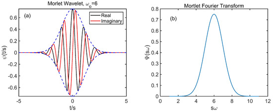
Figure 1.
(a) The Morlet wavelet in the time domain: the real part is in blue and the imaginary in red. (b) The Morlet wavelet in the frequency domain (see also Figure 2 in Torrence and Compo [41]).
The advantage of this wavelet being complex valued is that the CWT provides both amplitude and phase of the time series being analysed [50]. Furthermore, the similarity of the Morlet wavelet expansion to the Gabor transform, mentioned in Section 2.1, extends to the minimization of the product of uncertainties () [39]. An example of a wavelet spectrum utilizing the Morlet wavelet is shown in Figure 2.
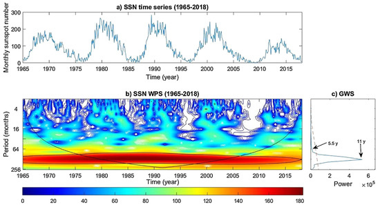
Figure 2.
Example of a wavelet powerspectrum on the Sunspot number time-series. (a) Time-series of the daily values of sunspot number. (b) Wavelet power spectrum; the wavelet power display is colour-coded with red corresponding to the maxima, while the black contour is the cone of influence of the spectra, where edge effects in the processing become important. (c) Global wavelet spectrum and its confidence level (dashed line) above 95%. Source: Tsichla et al. 2019 [51].
The average of the wavelet power spectral density is the global wavelet spectrum (panel c in Figure 2) and is given by:
The global wavelet spectrum is an unbiased and consistent estimation of the true power spectrum of a time series and generally exhibits similar features and shape as the corresponding Fourier spectrum.
The need for tests that are able to distinguish statistically significant results from those due to random background fluctuations (significance tests) is an essential prerequisite to any interpretation attempt regarding the results obtained from the application of CWT (or FT) on a single data sample. Hence, an appropriate background model is required for this task; white and red-noise spectra are often used [41]. This is justified, as the time series of interest usually exhibit higher variability in the long wavelengths than in the short. Under the circumstances of the null hypothesis (purely random results), the time-series used in the wavelet spectrum calculation is generated by uni-variate lag-1 autoregressive–AR(1) or Markov–process.
where weights the autoregressive term, is taken from Gaussian white noise (GWN) and power spectrum is [41,49]:
where k = 0 …N/2 is the frequency index.
As in [41,42] the test for , significant at p or, equivalently within a confidence level of , is performed based on the height of a wavelet power spectral peak above the background defined in Equation (5); the wavelet power spectral density is shown in Torrence and Compo [41] to be distributed with two degrees of freedom due to the two parts, real and imaginary, of this WT transform. If the variance of the time series is equal to the product is the theoretical wavelet power, which can then be compared with for the computation of the confidence intervals for the peaks in a wavelet power spectrum (see [41,49]):
where indicates “probability of X”, and the significance is p where, after a time honoured tradition, for the 95% confidence interval.
In the example presented in panel (c) of Figure 2, the 95% significance level is depicted in the plot of the peaks of the global wavelet spectrum; likewise, in Figure 3. Lastly, it needs to be noted that the application of a based criterion presupposes a close to a Gaussian distribution of the time series , [41]; in the case that the time series is far from Gaussian, some type of transformation must be considered, as suggested by Grinsted et al. [49].
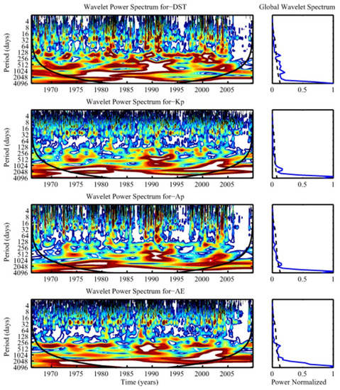
Figure 3.
Wavelet spectra and the normalised global wavelet spectra of geomagnetic indices (top to bottom): Dst, Kp, Ap and AE (Vsw). The wavelet spectra are colour-coded with red corresponding to the maxima; the black contour is the cone of influence of the spectra, where edge effects in the processing become important. The dashed lines in the global spectra represent a confidence level above 99%. Adapted from Katsavrias et al. 2012 [10].
The Continuous Wavelet Transform, presented in this section, is an effective method for the detection of the frequency and time structure of activity bursts, ubiquitous in most astrophysical and geophysical time-series. The study of the interactions of two or more time series, on the other hand, necessitates that this methodology is appropriately expanded; this is done in the following Section 2.2.2.
2.2.2. Cross Wavelet Transform (XWT) and Wavelet Coherence (WTC)
The Cross Wavelet Transform (XWT) extends the application of the CWT in the case of two or more time series (let them be X and Y); it underlines regions of coincident energy between signals and detects relative phase. It is, thus, a useful a wavelet–based method of investigation of the possibility of causal relationships in the time frequency space between them. If and are the CWTs of X and Y, the cross-wavelet transform is defined as [40,41,42,49]:
with denoting complex conjugate.
The result is, in general, complex, and its magnitude (or modulus) and phase (or argument) are examined separately; the modulus, , of the Wavelet Cross Spectrum indicates the covariance at scale and the non-dimensional time parameter n marks regions in the (t-f) space of high common power. The phase spectrum, obtained from , of the XWT represents the relative phase difference between the time-series to be compared [41,49]:
From the phase of the XWT the Wavelet Coherence, as a quantitative measure of the phase consistency (WTC) between and , will be derived in the remaining part of this section. It is noted in advance that the regions of high common power and consistent phase relationship indicate a possible causal relationship between X and Y.
The estimation of the significance of wavelet cross power peaks is distinctly similar to that of the wavelet spectral peaks outlined in Section 2.2.1. The red noise assumption, Equation (6), is used in the derivation of the null hypothesis and the estimates of the power spectra theoretical distributions and ; the computation of the confidence intervals is provided in (Grinsted et al. [49] Equation (5)) (also (Torrence and Compo [41] Equation (31))):
where k is the frequency index and equals 1 if the wavelet in use is real valued and 2 if it is complex valued. The function is the confidence level associated with the significance p for a probability distribution function defined as the square root of the product of two distributions each corresponding to and respectively; for example and ((Torrence and Compo [41] Section 6c), see also [49]).
The Wavelet Coherence (WTC) is an estimator of the confidence level for each detection of a time–space region of high common power and consistent phase relationship between two time-series calculated by means of the Cross Wavelet Transform (Equation (8)). The measure of wavelet coherence is defined between two continuous wavelet transforms, and this may indicate coherence with high confidence level even though the common power is low; it closely resembles a localized correlation coefficient in time–frequency space and varies between 0 and 1. It is used alongside the Cross Wavelet Transform, as the latter appears to be unsuitable for significance testing the interrelation between two processes [52]. Following (Torrence and Webster [42] see Appendix) and Grinsted et al. [49], we define the wavelet coherence of two time series—let them be X and Y:
where S is a smoothing operator and . The definition closely resembles that of a traditional correlation coefficient, which, in this case, is localized in the time frequency space. The smoothing operator S may be in the form:
where denotes smoothing along the wavelet scale axis and smoothing in time. The smoothing operator is expected to have, by design, a footprint as small as the wavelet used (see (Grinsted et al. [49] Equation (10)) for the analytical expression of a smoothing operator for the Morlet wavelet example, which was initially described in Torrence and Webster [42]).
The statistical significance level of the wavelet coherence is estimated using Monte Carlo methods as described in Grinsted et al. [49].
3. Application of Wavelet Methods
The solar wind–magnetosphere coupling forces the geomagnetic field perturbations as it provides the necessary energy input, with the results manifesting themselves as geomagnetic activity. The variability in the solar magnetic field, interacting with the magnetosphere at multiple time scales, which correspond to different processes, is a major driver of this coupling. In this section, we discriminate the periodic behaviour of the geomagnetic field in large-scale, i.e., periodicities larger than 27 days (solar rotation) and short-scale, i.e., geomagnetic oscillations in the timescale of the order of seconds (Ultra Low Frequency waves–ULF).
3.1. Application of Wavelet Methods in Large–Scale Periodic Behaviour
3.1.1. Geomagnetic Field
As already mentioned in the introduction, the solar wind is modulated by the solar activity variations; its interaction with the terrestrial magnetosphere introduces the solar-terrestrial coupling, which appears as the geomagnetic activity dependence on solar activity fluctuations. Quantitative measures of the former are the geomagnetic indices, such as Ap, Kp, aa and Dst, as well as the auroral indices AE, AL and AU (see Mayaud [53] and Menvielle et al. [54] for a review). Many publications have been dedicated to the study of time-variations of geomagnetic activity indices.
Following the initial work of Bartels [55] discussing the time variation of geomagnetic activity indices Kp and Ap during 1932–1961, Fraser-Smith [56] used FFT analysis on a 38-year period (1932–1969) of Ap data and obtaining prominent peaks at 10.2, 7.04, 5.14, 4.10, 1.47, 1.09 and 0.5 years, as well as prominent peaks at 27.2, 27.6 days and moderate peaks at 54.0, 37.4, 30.5, 26.9, 18.7, 14.1, 13.7, 13.6 and 9.39 days.
As wavelet methods became popular in the 1990s, several articles were focused on the study of the interconnection of geomagnetic activity with the variation of solar energetic events and of solar wind parameters in various time-scales; the detection of shared periodicities provided evidence in support of this interconnection [10].
The ∼27-day periodicity, linked to the solar rotation, has been detected in all geomagnetic indices [10,57]. The second and first harmonic (∼9 and ∼13.5 days) have been also detected, and they were associated with the presence of two high speed streams per solar rotation at 1 AU [7].
Lou et al. [58] detected, using CWT, seasonal variations in the Ap index of 187, 273 and 364 days in the 1999–2003 period. They interpreted the annual and semi-annual quasi-periodic oscillations in terms of CME-magnetosphere interactions. For the explication of the 273 days (∼0.7 years) periodicity, on the other hand, they used estimates for periodic time-scales of equatorially trapped Rossby-type waves [3]. Using a significantly extended dataset, spanning four solar cycles in the 1966–2010 time period, Katsavrias et al. [10] detected time-localized common spectral peaks, between the fluctuations in the solar wind characteristics and the geomagnetic indices, which corroborated some of the previously found periodicities.
On the contrary, the prominent semi-annual periodicity detected in the Dst index (and less prominent in the Kp index) did not appear to have originated in the Solar wind parameter fluctuation (Figure 3). Therefore, it was attributed to reconnection processes in the day-side magnetosphere induced by the Russell and McPherron [59] effect. Furthermore, contrary to the Ap periodicity reported in Lou et al. [58], the AE index was found to have only an annual peak.
Nayar et al. [8] reported Quasi-Biennial Oscillations (QBO) of the geomagnetic activity index Ap; 1.3–1.4 years during even cycles and of 1.5–1.7 years during odd ones, likely propagating from the solar magnetic field (SMF) and were associated with double peaks of the solar cycle. These double peaks were attributed to a superposition of the usual 11-year cycle and wave trains with periodicities continuously varying from three years at solar maximum, to 1.7 years towards solar minimum [5].
A step further, Ou et al. [60] examined the second-order time derivatives derived from monthly means of the X, Y and Z field components recorded by the global network of ground-based observatories between 1985–2010. Having filtered out very high and very low frequency components (due to the use of the monthly mean and of the time-series derivative, respectively), they identified five principal periods at 1.3, 1.7, 2.2, 2.9 and 5.0 years.
The authors suggested that, even though QBOs in the geomagnetic field are generated from a common source (very high correlation between the geomagnetic QBO and the QBOs in solar wind speed and solar wind dynamic pressure), their features indicate that they primarily originate from the various current systems related to the solar wind-magnetosphere-ionosphere coupling process. The dependence of geomagnetic indices on the interplanetary magnetic field (IMF) polarities, toward and away (T and A, respectively) has been also investigated by utilizing wavelet analysis [61,62]. The results showed a significant N-S asymmetry of these indices, depending on the solar cycles.
In an attempt to link the quasi-periodic variations exhibited by the geomagnetic activity with the solar wind parameters, Andriyas and Andriyas [63] used wavelet analysis to study the interrelationship between ten solar wind coupling functions with the geomagnetic indices Dst and AL. The authors indicated that no single coupling function could explain the variances in geomagnetic indices at all the time-scales. Moreover, the authors observed that although there were periodicities common to the coupling functions and the AL index, the amount of correlation was poor when compared to the Dst index.
As already mentioned, the quasi-periodic behaviour of the geomagnetic activity is more complex than the that exhibited by solar activity parameters. This is due to the fact that the former is driven by two dominant drivers: (a) the high speed solar wind streams from coronal holes and (b) the intermittent solar activity (eruptive events). Feynman [11] was the first to compare aa index variations with sunspot numbers and, since the solar wind drives the geomagnetic activity, concluded that the 11-year solar cycle, as represented by the sunspot numbers, was very different from the one represented by the solar wind parameters and geomagnetic indices.
In particular, on annual scale, the geomagnetic index aa could be the result of two components: one originating from solar transient (or sporadic) activity and in phase with the solar cycle; the other was related to recurrent solar drivers with peak in the descending phase. The major driver of transient geomagnetic activity is the Interplanetary Coronal Mass Ejections (ICME). The solar recurrent activity, on the other hand, is driven by High Speed Solar Wind Streams (HSSWS) and Stream Interaction Regions (SIR).
Taking another step further, Katsavrias et al. [13] used cross-wavelet transform (XWT) and wavelet coherence (WTC) to study the relationship between transient and recurrent phenomena, i.e., ICMEs and CIRs and the corresponding magnetospheric response represented by geomagnetic indices Dst and AE, during the solar cycle 23. The authors verified that CIRs modulate the geomagnetic response during the ascending and descending phase, while ICMEs during the maximum of the cycle and the unusual active period of 2002–2005; nevertheless, this feature was evident in the 27-day periodic component only (Figure 4).
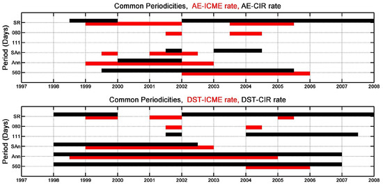
Figure 4.
Common periodicities between geomagnetic indices (AE in the upper panel and DST in the lower panel) and drivers, as detected by the XWT. The red lines correspond to ICMEs and the black to CIR. The y-axis labels SR, SAn and Ann stand for Solar Rotation, Semi-Annual and Annual periodicities. Source: Katsavrias et al. 2016 [13].
3.1.2. Magnetospheric Particles and Cosmic Rays
As already mentioned, the seasonal variation (annual and semi-annual) has long been recognized in geomagnetic activity. The discovery of the trapped particle populations in the inner magnetosphere (Van Allen radiation belts) opened a brand new scientific domain, which led to the launch of several scientific space missions in the 1990s. One of them, the Solar Anomalous and Magnetospheric Particle Explorer (SAMPEX) satellite, gave the appropriate measurements in order for the semi-annual variation (SAV) in the electron fluxes of the outer radiation belt to be discovered [64]. The nature of this variation were under debate for several years, as three possible mechanisms had been proposed:
- 1.
- The axial effect [65], which is due to the variation of the position of the Earth in heliographic latitude.
- 2.
- The equinoctial effect [66], as a consequence of the varying angle of the Earth’s dipole with respect to the Earth-Sun line.
- 3.
- The Russell and McPherron [59] effect, a result of the larger z component of the interplanetary magnetic field (IMF) near the equinoxes in GSM coordinates, owing to the tilt of the dipole axis relative to the heliographic equatorial plane.
With the aid of wavelet methods Katsavrias et al. [67] linked the semi-annual variation to the Russell–McPherron effect: They used electron flux measurements from the Van Allen probes and Geostationary Operational Environmental Satellites (GOES) and performed cross-wavelet analysis with respect to the angles of the three proposed mechanisms. The calculated XWT and WTC spectral peaks indicated an in-phase relationship between the electron flux and the angle that controls the Russell–McPherron effect (Figure 5) at the ∼178 days periodicity. The same result was verified by other methods by Poblet et al. [68].
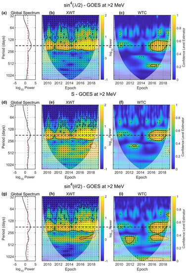
Figure 5.
Global wavelet (a,d,g), cross-wavelet transformation (XWT; b,e,h) and wavelet coherence (WTC; c,f,i) between the >2 MeV electron flux from GOES/EPS and the function (a–c) that controls the axial effect, the S function (d–f) that controls the equinoctial effect and the function (g–i) that controls the Russell–McPherron; the dashed red line corresponds to the 95% confidence level of the global wavelet. The thick black contours mark the 95% confidence level, and the thin line indicates the cone of influence (COI). The colour bar of the XWT indicates the log10 (power); the colour bar of the WTC corresponds to the confidence level of the phase obtained by the Monte Carlo test, and the arrows correspond to a confidence level > 0.6. The arrows point to the phase relationship of the two data series in time–frequency space: (1) arrows pointing to the right indicate in-phase behaviour; (2) arrows pointing to the left indicate anti-phase behaviour; (3) arrows pointing downward indicate that the first dataset is leading the second (meaning that the first dataset occurs earlier in time) by 90. The horizontal dashed (black) lines highlight the SAV. Source: Katsavrias et al. 2021 [67].
In addition, wavelet analysis revealed that the semi-annual variation was more pronounced during the descending phases of Solar cycles 22, 23 and 24 and, moreover, coexisted with periods of increased number of High Speed Streams (HSSWS) and decreased the Interplanetary Coronal Mass Ejections (ICME) occurrence, indicating that the SAV was a result of the modulation of reconnection produced by the variability of the controlling angles of the RM (and/or equinoctial) mechanism during periods of enhanced solar wind speed.
The aforementioned results were of significant importance to the outer radiation belt dynamics, since the angle, , that controls the Russell–McPherron effect has been proven crucial for the prediction of the long-term variability of energetic electron fluxes [69].
Several large-scale periodicities have been also detected in the cosmic ray (CR) time-series. Galactic cosmic rays (GCRs) are energetic charged particles, spanning a broad range in energy (10–10 eV/nucleon), mostly with an out-of-solar-system origin. These high-energy GCRs can reach the Earth’s atmosphere and trigger particle and electromagnetic cascades, thereby, creating a great variety of secondary particles, such as neutrons, which can be measured by ground-based neutron monitors [51]. The transport of GCR in the heliosphere, as of all charged particles, is known to be influenced and controlled by the spatial and temporal distribution of the interplanetary magnetic field (IMF). Therefore, the GCR evolution is expected to share common periodic behaviour with solar/solar wind parameters.
Except for the well-known 11-year periodicity due to the solar cycle and the annual variations, peaks at 7.7, 5.5, 2 and 1.7 years have been found by Mavromichalaki et al. [70]. The authors used wavelet analysis to indicate that the period of 7.7 years was related to the 22-year cycle and consequently, with the polarity of the solar magnetic field. On the other hand, the period of 5.5 years was related to the enhanced power of the second harmonic, which arises from the asymmetric form of the 11-year solar cycle.
QBOs are also very prominent in neutron monitor data. In an extensive study using wavelet analysis, Kudela et al. [71] showed that, while a dominant quasi-periodicity centring at ∼1.7 years–was exhibited during the odd cycle 21 (1981-1984), there was an enhanced contribution from the 1.3 years quasi-periodicity during the even cycles 20 and 22.
Even though the aforementioned variations are linked with the solar activity dynamics, shorter-scale periodicities are linked with transient phenomena in the interplanetary space. Chowdhury et al. [72] detected significant periods in the range of 8–32 days including a solar rotational period of approximately 27 days, as well as prominent Rieger-type periodicities, during the maximum of solar cycle 24, associated with Solar eruptive events (Figure 6).
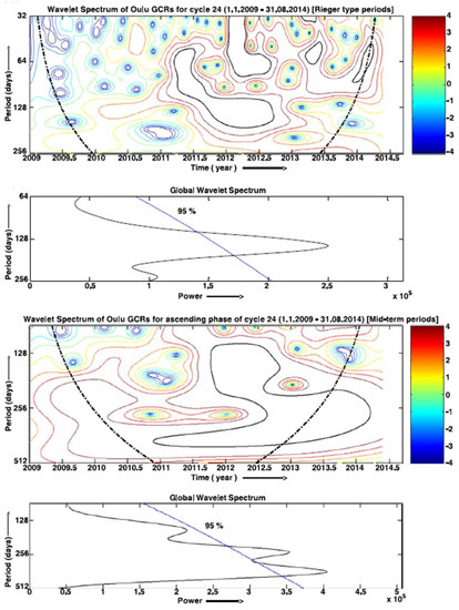
Figure 6.
Pairs of panels showing localand global wavelet spectra of GCRs for January 2009–August 2014 in successive periodicity ranges: (top panels) in the range of 32–256 days for studying mainly Rieger-type quasi periodicities; and (bottom panels) in the range of 128–512 days for studying QBOs. In all the panels, the 95% confidence levels in the local wavelet spectra are shown by thin black contours and those in the global wavelet spectra are shown by blue dash-dot lines. The thin black contours within the COI show the periodicities above the 95% confidence level. Source: Chowdhury et al. 2016 [72].
3.2. Application of Wavelet Methods in Short–Scale Periodic Behaviour
3.2.1. Ultra-Low Frequency Waves
Over the past decades, it has been well established that a geospace disturbance is the consequence of a geo-effective solar wind flow reaching the near-Earth space environment. These disturbances are associated with the variability of charged particles in the Earth’s radiation belts and the intensification of electric current systems with characteristic signatures on the geomagnetic field [73]. Periodic oscillations in the Earth’s magnetic field with frequencies in the range of a few millihertz (ultra low frequency ULF waves) can significantly influence radiation belt dynamics due to their potential for strong interactions with charged particle populations.
In particular, the ULF waves in the Pc4-5 band (1–25 mHz) can violate the third adiabatic invariant L of the energetic electrons. This drives radial diffusion by conserving the first two adiabatic invariants under the drift resonance condition , where is the wave frequency, m is the azimuthal wave mode number and is the electron drift frequency [74]. Radial diffusion is one of the most important mechanisms, since it has a dual role; it can lead to both energization [75,76,77,78,79] and loss of relativistic electrons [80,81,82].
ULF waves have been traditionally identified through the visual inspection of series of spectrograms based on the Fast Fourier Transform (FFT) or by the application of simple, automated or semi-automated (i.e., requiring some amount of human intervention) techniques [83,84]. Since the 1990s, wavelet spectral analysis has become popular, as it allows the quantitative monitoring of localized variations of power within the time series data [85]. Moreover, wavelet analysis can be superior to the Fourier spectral analysis when the spectral properties of transient, impulsive, short-lived or non-stationary signals need to be analysed, especially when the nature of the investigated signal is not a priori known.
An appropriate selection of the mother function allows for better detection of these signals and does so in a direct way, without the need for a moving window and the many arbitrary choices that arise from it, such as its length, step, envelope function and so on. This also produces outputs that are significantly smoother and thus allows for the better application of thresholds and more accurate identification of fast and short-scale phenomena. This is also evident by the series of studies that have highlighted the significance of applying wavelet analysis and especially its suitability for multipoint, small-scale disturbances, in the investigation of ULF wave events.
Wavelet analysis has been further used in the development of automated algorithms for the detection of ULF waves. Heilig et al. [86] developed an algorithm for the selection of possible upstream wave related pulsation events (frequencies in the 20–80 mHz range) from both ground and space magnetometer data. Balasis et al. [87] developed a time–frequency analysis tool for automated detection of ULF wave events in magnetic and electric field measurements made from multi-satellite missions and ground-based networks.
The Pc3 waves (in the 20–100 mHz frequency range) were identified by examining series of time–frequency spectrograms, produced with wavelet-based algorithms. This detection tool was later on implemented in a machine-learning-based model in order to detect ULF waves in the time series of the magnetic field measurements on board the low-Earth orbit CHAMP satellite [88]. Furthermore, Papadimitriou et al. [89] exploited this detection tool to create maps of Pc3-4 ULF wave power (in the 10–100 mHz frequency range–see also Figure 7) and a ULF wave index, which was then correlated with the solar wind parameters to elucidate the driving factors behind the onset and propagation of these waves.
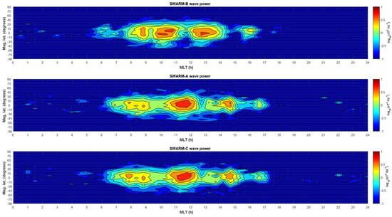
Figure 7.
Swarm Pc3 wave powermap in magnetic coordinates. Pc3 wave power per second mapped on the magnetic latitude versus MLT grid. Source: Papadimitriou et al. 2018 [89].
The ability of the wavelet transform to characterize both the frequency and temporal content of waves makes it ideal for studying irregular pulsations (Pi1 and Pi2), as well. Especially, Pi2 ULF waves (7–25 mHz) are intimately connected with the onset of the expansion phase during magnetospheric substorms. Therefore, efforts have been devoted to the development of automated algorithms, utilizing a wavelet power threshold for Pi2 waves, for nowcasting/forecasting magnetospheric substorms from real-time ground-based magnetometer data [90] and ultraviolet images [91].
Wavelet analysis has also been applied in the detection of causal relations between the magnetosheath pressure and the waves observed in the magnetosphere. Archer et al. [92], investigated the impact of large amplitude, transient dynamic pressure pulses on the generation of compressional and poloidal mode waves (Pc5-6 frequency range) in the outer magnetosphere. They also used the cross-wavelet transform and wavelet coherence in order to detect the generation of well-defined standing waves (90 phase relationship with coherence levels higher than 0.75). Using wavelet analysis, Archer et al. [93] showed that broadband jets in the subsolar magnetosheath directly and resonantly drive ULF waves in the magnetosphere at the so-called magic frequencies (roughly 0.7, 1.3, 1.9, 2.6, 3.3 and 4.8 mHz) as well as local field line resonances.
Another characteristic example of the use of wavelet methods in the magnetosheath–magnetosphere coupling is the work of Katsavrias et al. [94]. The latter authors used multipoint magnetic field observations to detect identical Pi2 pulsations in the magnetosheath (similar to the ones accompany substorm onsets), generated at the wake of a jet and in the outer magnetosphere. Using cross-wavelet analysis and wavelet coherence, showed that the phase difference between the two pulsations was in good agreement with the propagation time of a disturbance travelling with Alfvnic speed, indicating that they are directly related.
3.2.2. Radial Diffusion of the Trapped Electron Population in the Outer Radiation Belt
In the previous section, we discussed the importance of ULF waves, in the variability of the trapped electron population in the outer radiation belt, as drivers of the radial diffusion processes. The quantification of these processes is possible through the estimation of the radial diffusion coefficient (D), which represents the mean square change of the drift-shell (L) for a large number of particles over time. According to Fei et al. [95], the D is the sum of the effects of perturbations in the azimuthal electric field and the parallel magnetic field:
These two components of the radial diffusion coefficients are given by:
where is the first adiabatic invariant, L is the Roederers L, q is the charge of the diffused electrons, is the Lorentz factor, is the Earth’s radius and is the strength of the equatorial geomagnetic field on the Earth’s surface. Moreover, P corresponds to the wave power at a specific drift frequency () for all the azimuthal mode numbers (m).
It is clear, from this formulation (Equations (14) and (15)), that accurate calculations of the D require equally accurate spectral analysis of the magnetic and electric field measurements used in the computation of the Power Spectral Density (PSD) of the Pc4-5 ULF waves. Since the temporal evolution of the PSD is of outmost importance for the calculation of the D, wavelet analysis is one of the most commonly used methods [96,97,98,99,100].
4. Revisiting the Estimation of Wavelet PSD and Comparison with FFT
One of the most often-heard criticisms of wavelet analysis is that, for most cases, the mother wavelets do not form an orthonormal basis, meaning that their inner product for frequencies at different octaves, i.e., at frequencies with ratios that are integer powers of two, is not zero [101]. Even though, this is technically true, for a careful choice of the mother function and its parameters, the derived wavelets can be quasi-orthogonal, in the sense that even if their product is not exactly zero, it is a very small number that can be safely approximated by zero.
As an example, by choosing the value of 6 for the parameter of the Morlet wavelet (Equation (2)), the inner product of the generated wavelets is smaller than and so can be considered zero for all practical applications.
A second argument against wavelets is that the derived wave power depends on the values of the parameters employed in the methodology—something that makes comparisons against other methods and particularly against spectra derived by means of the FFT problematic. This becomes even more important when the results of the analysis are being used as inputs for the calculation of other quantities, such as the radial diffusion coefficients discussed in Section 3.2.2 above. This is a critical issue as the differences between even small changes in the parameters can be quite substantial; however, it can also be alleviated by applying the proper normalization technique. Note that the corresponding code for the estimation of PSD using this normalization technique is publicly available at https://synergasia.uoa.gr/modules/document/index.php?course=PHYS120 accessed on 9 March 2022.
To examine all these and better illustrate this method, we produce an artificial signal, to be used as the benchmark for the tests to follow. The signal is a modulated sinusoidal, with a time-varying frequency and some additive noise and is given by:
with varying linearly from 1 up to 125 mHz, being Gaussian random noise with a mean of zero and standard deviation of 1 and the exponential term signifying a Gaussian envelope in the amplitude of the sinusoidal. The signal was constructed as a series of 20,000 points with a sampling time of = 4 s, so that with n from 1 up to 20,000 and can be seen at the top panel of Figure 8.
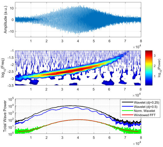
Figure 8.
Test signal (top panel) along with its wavelet time–frequency analysis (middle panel) and its total power with respect to time (bottom panel), computed by various methods.
To compute the wavelet spectrum of this signal, the Torrence & Compo code was used, with the Morlet mother function and an . To define the scales (and correspondingly the frequencies) on which the analysis will be performed, we used the convention in the same publication [41] to construct 37 scales, starting from , which practically corresponds to the Nyquist frequency for this test signal and using a scale step dj of 0.25, implying that we generate four scales for each octave. The scales themselves follow the relation , with m from 0 up to 36, which yields scales from sec up to 16,384 s. The wavelet power of the signal under these parameters is shown in the middle panel of Figure 8, from which we can see both the rising tone characteristic of this signal and its initially increasing and afterwards diminishing amplitude.
To compare against Fourier spectra, we perform a windowed-FFT analysis, by using a moving window of 900 points, i.e., one hour in duration, moving it by a step of only one point each time and computing the Fourier spectrum on the same range of frequencies as for the wavelet case, taking into account the relation between the two as given in Equation (3). The orthogonality of the Fourier transform and the conservation of the signal energy that it implies, allows us to compute the sum of the squares of the magnitude of the Fourier coefficients, along this frequency range and obtain a total wave power for each point in time. Doing naively the same for the wavelet case produces results that differ significantly from the FFT ones.
As the frequencies themselves can be chosen almost arbitrarily for the wavelet case, we can obtain different results even using a different frequency resolution dj, since the summation will now extend to more frequencies on which the wavelet representation is highly correlated. All these points are easily illustrated in the bottom panel of Figure 8, where the blue and black curves correspond to the sum of the wave power for the wavelet method (one with dj = 0.25 and the other of dj = 0.5), while the red curve to the result of the windowed FFT analysis. Thankfully, the normalization that is given in (Torrence and Compo [41] Equation (14)) provides us with the way to re-introduce the conservation of the signal’s energy in the wavelet formalism, so now the Total Wave Power for each moment in time can be computed as:
with an empirically derived factor that for the Morlet case (with ) is equal to 0.776. By following this normalization, the total power along all frequencies examined in this example produces the green curve, which matches perfectly the red curve, which was the result of the windowed FFT analysis. Hence, by revisiting and adopting a normalization approach suggested more than 20 years ago (but overlooked in many modern wavelet studies involving space physics data), we are able to conserve the energy of the time series under analysis in the time–frequency domain using the wavelet transform.
Applying this normalization allows the full arsenal of the wavelet methodology and all its benefits to be used in a robust and consistent way for the estimation of the wavelet power spectral density within a specific frequency range and with respect to time, so that other parameters that are based on it, e.g., the radial diffusion coefficients, can now be accurately derived and compared with those that are procured from more traditional, Fourier-based methods. Especially for the radial diffusion coefficients case, the calculation of the wavelet power spectral density that is needed for their calculations can now immediately be achieved by dividing the total wave power by the step in frequency range , hence .
5. Summary
In this review, we highlighted the significant contributions of the wavelet methods in the research of solar-terrestrial coupling and geospace disturbances. Wavelet analysis can be superior to other methods for spectral analysis since its time-localization allows for the better detection of non-stationary signals (especially when their nature is not a priori known), without the need for a moving window and the many arbitrary choices that arise from it.
Since, the 1990s, wavelet methods have been applied in the accurate identification of not only fast and short-scale phenomena, such as ULF waves (geomagnetic oscillations in the timescale of the order of seconds) and the subsequent radial diffusion coefficients, but also in the identification of a variety of large-scale phenomena (periodicities larger than 27-day solar rotation) in the Sun, the solar wind, the geomagnetic field, the trapped particle population in the inner magnetosphere and cosmic rays.
Finally, we presented an optimal approach for the accurate estimation of the PSD that is compatible with the results obtained from FFT analysis, highlighting how wavelets can be used consistently regardless of the choice of mother function or other parameters. The corresponding code for the estimation of PSD using the aforementioned method is publicly available at https://synergasia.uoa.gr/modules/document/index.php?course=PHYS120 accessed on 9 March 2022.
Author Contributions
Conceptualization, C.K.; software, C.P.; investigation, C.K., C.P. and A.H.; writing—original draft preparation, C.K., C.P., A.H. and G.B.; writing—review and editing, C.K., C.P., A.H. and G.B. All authors have read and agreed to the published version of the manuscript.
Funding
This research received no external funding.
Institutional Review Board Statement
Not applicable.
Informed Consent Statement
Not applicable.
Data Availability Statement
No data available.
Acknowledgments
The authors acknowledge the support and funding from the European Union’s Horizon 2020 research and innovation programme “SafeSpace” under grant agreement No 870437. The authors also thank the guest editors Panagiota Preka-Papadema and Xue Liang for the invitation to this special issue.
Conflicts of Interest
The authors declare no conflict of interest.
Abbreviations
The following abbreviations are used in this manuscript:
| CHAMP | CHAllenging Minisatellite Payload |
| CIR | Corotating Interaction Region |
| CME | Coronal Mass Ejection |
| COI | Cone of Influence |
| CR | Cosmic Rays |
| CWT | Continuous Wavelet Transform |
| DWT | Discrete Wavelet Transform |
| FFT | Fast Fourier Transform |
| FT | Fourier Transform |
| GCR | Galactic Cosmic Rays |
| GOES | Geostationary Operational Environmental Satellite |
| GSM | Geocentric Solar Magnetospheric |
| GWN | Gaussian White Noise |
| HSSWS | High Speed Solar Wind Stream |
| ICME | Interplanetary Coronal Mass Ejection |
| IMF | Interplanetary Magnetic Field |
| Pc | Pulsation continuous |
| Pi | Pulsation irregular |
| PSD | Power Spectral Density |
| RM | Russell–McPherron |
| SAMPEX | Solar Anomalous and Magnetospheric Particle Explorer |
| SAV | Semi-Annual Variation |
| SIR | Stream Interaction Region |
| SMF | Solar Magnetic Field |
| STFT | Short-Time Fourier Transform |
| ULF | Ultra-Low Frequency |
| WTC | Wavelet Coherence |
| XWT | Cross Wavelet Transform |
| QBO | Quasi-Biennial Oscillation |
References
- Hathaway, D.H. The Solar Cycle. Living Rev. Sol. Phys. 2010, 7, 1–87. [Google Scholar] [CrossRef]
- Rieger, E.; Share, G.H.; Forrest, D.J.; Kanbach, G.; Reppin, C.; Chupp, E.L. A 154-day periodicity in the occurrence of hard solar flares? Nature 1984, 312, 623625. [Google Scholar] [CrossRef]
- Dimitropoulou, M.; Moussas, X.; Strintzi, D. Enhanced Rieger-type periodicities detection in X-ray solar flares and statistical validation of Rossby waves existence. Mon. Not. R. Astron. Soc. 2008, 386, 22782284. [Google Scholar] [CrossRef]
- Polygiannakis, J.; Preka-Papadema, P.; Petropoulos, B.; Pothitakis, G.; Moussas, X.; Pappas, G.; Hillaris, A. Ephemeral periodicities in the solar activity. In SOLMAG 2002, Proceedings of the Magnetic Coupling of the Solar Atmosphere Euroconference, 11–15 June 2002, Santorini, Greece; Sawaya-Lacoste, H., Ed.; ESA Special Publications: Noordwijk, The Netherlands, 2002; Volume 505, pp. 537–540. [Google Scholar]
- Polygiannakis, J.; Preka-Papadema, P.; Moussas, X. On signal-noise decomposition of time-series using the continuous wavelet transform: Application to sunspot index. Mon. Not. R. Astron. Soc. 2003, 343, 725734. [Google Scholar] [CrossRef]
- Gazis, P.R.; Richardson, J.D.; Paularena, K.I. Long term periodicity in solar wind velocity during the last three solar cycles. Geophys. Res. Lett. 1995, 22, 11651168. [Google Scholar] [CrossRef]
- Mursula, K.; Zieger, B. The 13.5-day periodicity in the Sun, solar wind, and geomagnetic activity: The last three solar cycles. J. Geophys. Res. Space Phys. 1996, 101, 2707727090. [Google Scholar] [CrossRef]
- Nayar, S.P.; Radhika, V.; Revathy, K.; Ramadas, V. Wavelet Analysis of solar, solar wind and geomagnetic parameters. Sol. Phys. 2002, 208, 359373. [Google Scholar] [CrossRef]
- Bolzan, M.J.A.; Rosa, R.R.; Ramos, F.M.; Fagundes, P.R.; Sahai, Y. Generalized thermostatistics and wavelet analysis of solar wind and proton density variability. J. Atmos. Sol.-Terr. Phys. 2005, 67, 18431851. [Google Scholar] [CrossRef]
- Katsavrias, C.; Preka-Papadema, P.; Moussas, X. Wavelet Analysis on Solar Wind Parameters and Geomagnetic Indices. Sol. Phys. 2012, 280, 623640. [Google Scholar] [CrossRef]
- Feynman, J. Geomagnetic and solar wind cycles, 1900 1975. J. Geophys. Res. 1982, 87, 6153. [Google Scholar] [CrossRef]
- Du, Z.L. The Solar Cycle: A new prediction technique based on logarithmic values. Astrophys. Space Sci. 2011, 338, 913. [Google Scholar] [CrossRef][Green Version]
- Katsavrias, C.; Hillaris, A.; Preka-Papadema, P. A wavelet based approach to SolarTerrestrial Coupling. Adv. Space Res. 2016, 57, 22342244. [Google Scholar] [CrossRef]
- Valdes-Galicia, J.F.; Perez-Enriquez, R.; Otaola, J.A. The cosmic-ray 1.68-year variation: A clue to understand the nature of the solar cycle? Sol. Phys. 1996, 167, 409417. [Google Scholar] [CrossRef]
- Kudela, K.; Mavromichalaki, H.; Papaioannou, A.; Gerontidou, M. On Mid-Term Periodicities in Cosmic Rays. Sol. Phys. 2010, 266, 173180. [Google Scholar] [CrossRef]
- Addison, P. The little wave with the big future. Phys. World 2004, 17, 3539. [Google Scholar] [CrossRef]
- Balasis, G.; Daglis, I.A.; Kapiris, P.; Mandea, M.; Vassiliadis, D.; Eftaxias, K. From pre-storm activity to magnetic storms: A transition described in terms of fractal dynamics. Ann. Geophys. 2006, 24, 3557–3567. [Google Scholar] [CrossRef]
- Mandea, M.; Balasis, G. The SGR 1806-20 magnetar signature on the Earth’s magnetic field. Geophys. J. Int. 2006, 167, 586–591. [Google Scholar] [CrossRef]
- Balasis, G.; Mandea, M. Can electromagnetic disturbances related to the recent great earthquakes be detected by satellite magnetometers? Tectonophysics 2007, 431, 173–195. [Google Scholar] [CrossRef]
- Kunagu, P.; Balasis, G.; Lesur, V.; Chandrasekhar, E.; Papadimitriou, C. Wavelet characterization of external magnetic sources as observed by CHAMP satellite: Evidence for unmodelled signals in geomagnetic field models. Geophys. J. Int. 2013, 192, 946–950. [Google Scholar] [CrossRef]
- Zaourar, N.; Hamoudi, M.; Mandea, M.; Balasis, G.; Holschneider, M. Wavelet-based multiscale analysis of geomagnetic disturbance. Earth Planets Space 2013, 65, 1525–1540. [Google Scholar] [CrossRef]
- Daubechies, I. Where do wavelets come from? A personal point of view. Proc. IEEE 1996, 84, 510513. [Google Scholar] [CrossRef]
- Farge, M. Wavelet transforms and their applications to turbulence. Annu. Rev. Fluid Mech. 1992, 24, 395–457. [Google Scholar] [CrossRef]
- Strang, G. Wavelet transforms versus Fourier transforms. Bull. Am. Math. Soc. 1993, 28, 288305. [Google Scholar] [CrossRef]
- Lee, D.T.; Yamamoto, A. Wavelet analysis: Theory and applications. Hewlett Packard J. 1994, 45, 4452. [Google Scholar]
- Lau, K.M.; Weng, H. Climate Signal Detection Using Wavelet Transform: How to Make a Time Series Sing. Bull. Am. Meteorol. Soc. 1995, 76, 23912402. [Google Scholar] [CrossRef]
- Graps, A. An introduction to wavelets. IEEE Comput. Sci. Eng. 1995, 2, 5061. [Google Scholar] [CrossRef]
- Akujuobi, C.M. Wavelets and Wavelet Transform Systems and Their Applications; Springer International Publishing: Berlin/Heidelberg, Germany, 2022. [Google Scholar] [CrossRef]
- Fourier, J.B.J. Théorie Analytique de la Chaleur; Chez Firmin Didot, Père et Fils: Paris, France, 1822. [Google Scholar]
- Kumar, P.; Foufoula-Georgiou, E. A multicomponent decomposition of spatial rainfall fields: 1. Segregation of large- and small-scale features using wavelet transforms. Water Resour. Res. 1993, 29, 2515–2532. [Google Scholar] [CrossRef]
- Foufoula-Georgiou, E.; Kumar, P. Wavelet Analysis in Geophysics: An Introduction. In Wavelets in Geophysics; Elsevier: Amsterdam, The Netherlands, 1994; p. 143. [Google Scholar] [CrossRef]
- Gabor, D. Theory of communication. Part 1: The analysis of information. J. Inst. Electr. Eng.-Part III Radio Commun. Eng. 1946, 93, 429441. [Google Scholar] [CrossRef]
- Daubechies, I. The wavelet transform, time–frequency localization and signal analysis. IEEE Trans. Inf. Theory 1990, 36, 9611005. [Google Scholar] [CrossRef]
- Rioul, O.; Vetterli, M. Wavelets and signal processing. IEEE Signal Process. Mag. 1991, 8, 14–36. [Google Scholar] [CrossRef]
- Russell, B.; Han, J. Jean Morlet and the continuous wavelet transform. CREWES Res. Rep. 2016, 28, 115. [Google Scholar]
- Priestley, M.B. Evolutionary Spectra and Non-Stationary Processes. J. R. Stat. Soc. Ser. B (Methodol.) 1965, 27, 204–229. [Google Scholar] [CrossRef]
- Lin, Y.K.; Cai, G.Q. Probabilistic Structural Dynamics; McGraw Hill Higher Education: Maidenhead, UK, 2004. [Google Scholar]
- Spatial Statistics and Digital Image Analysis; National Academies Press: Washington, DC, USA, 1991. [CrossRef]
- Morlet, J.; Arens, G.; Fourgeau, E.; Giard, D. Wave propagation and sampling theory Part II: Sampling theory and complex waves. Geophysics 1982, 47, 222236. [Google Scholar] [CrossRef]
- Addison, P. The Illustrated Wavelet Transform Handbook: Introductory Theory and Applications in Science, Engineering, Medicine and Finance, 2nd ed.; CRC Press: Boca Raton, FL, USA, 2017. [Google Scholar] [CrossRef]
- Torrence, C.; Compo, G.P. A Practical Guide to Wavelet Analysis. Bull. Am. Meteorol. Soc. 1998, 79, 61–78. [Google Scholar] [CrossRef]
- Torrence, C.; Webster, P.J. Interdecadal Changes in the ENSO-Monsoon System. J. Clim. 1999, 12, 2679–2690. [Google Scholar] [CrossRef]
- Kantelhardt, J.W. Fractal and Multifractal Time Series. In Encyclopedia of Complexity and Systems Science; Meyers, R.A., Ed.; Springer: New York, NY, USA, 2009; p. 37543779. [Google Scholar] [CrossRef]
- Kaiser, G. A Friendly Guide to Wavelets; Birkhäuser: Boston, MA, USA, 2011. [Google Scholar] [CrossRef]
- Astaf’eva, N.M. Wavelet analysis: Basic theory and some applications. Physics-Uspekhi 1996, 39, 10851108. [Google Scholar] [CrossRef]
- Novikov, I.Y.; Stechkin, S.B. Basic wavelet theory. Russ. Math. Surv. 1998, 53, 11591231. [Google Scholar] [CrossRef]
- Morlet, J. Sampling Theory and Wave Propagation. In Issues in Acoustic Signal Image Processing and Recognition; Springer: Berlin/Heidelberg, Germany, 1983; p. 233261. [Google Scholar] [CrossRef]
- Ashmead, J. Morlet Wavelets in Quantum Mechanics. Quanta 2012, 1, 5870. [Google Scholar] [CrossRef]
- Grinsted, A.; Moore, J.C.; Jevrejeva, S. Application of the cross wavelet transform and wavelet coherence to geophysical time series. Nonlinear Process. Geophys. 2004, 11, 561–566. [Google Scholar] [CrossRef]
- Kumar, P.; Foufoula-Georgiou, E. Wavelet analysis for geophysical applications. Rev. Geophys. 1997, 35, 385412. [Google Scholar] [CrossRef]
- Tsichla, M.; Gerontidou, M.; Mavromichalaki, H. Spectral Analysis of Solar and Geomagnetic Parameters in Relation to Cosmic-ray Intensity for the Time Period 1965–2018. Sol. Phys. 2019, 294, 15. [Google Scholar] [CrossRef]
- Maraun, D.; Kurths, J. Cross wavelet analysis: Significance testing and pitfalls. Nonlinear Process. Geophys. 2004, 11, 505–514. [Google Scholar] [CrossRef]
- Mayaud, P.N. Derivation, Meaning, and Use of Geomagnetic Indices. Wash. Am. Geophys. Union Geophys. Monogr. Ser. 1980, 22, 607. [Google Scholar] [CrossRef]
- Menvielle, M.; Iyemori, T.; Marchaudon, A.; Nosé, M. Geomagnetic Indices. In Geomagnetic Observations and Models; Springer: Dordrecht, The Netherlands, 2010; p. 183228. [Google Scholar] [CrossRef]
- Bartels, J. Discussion of time-variations of geomagnetic activity, indices Kp and Ap, 1932–1961. Ann. Geophys. 1963, 19, 1. [Google Scholar]
- Fraser-Smith, A.C. Spectrum of the geomagnetic activity indexAp. J. Geophys. Res. 1972, 77, 42094220. [Google Scholar] [CrossRef]
- Singh, Y.; Badruddin. Short- and mid-term oscillations of solar, geomagnetic activity and cosmic-ray intensity during the last two solar magnetic cycles. Planet. Space Sci. 2017, 138, 16. [Google Scholar] [CrossRef]
- Lou, Y.Q.; Wang, Y.M.; Fan, Z.; Wang, S.; Wang, J.X. Periodicities in solar coronal mass ejections. Mon. Not. R. Astron. Soc. 2003, 345, 809818. [Google Scholar] [CrossRef]
- Russell, C.T.; McPherron, R.L. Semi-annual variation of geomagnetic activity. J. Geophys. Res. 1973, 78, 92108. [Google Scholar] [CrossRef]
- Ou, J.; Du, A.; Finlay, C.C. Quasi-biennial oscillations in the geomagnetic field: Their global characteristics and origin. J. Geophys. Res. Space Phys. 2017, 122, 50435058. [Google Scholar] [CrossRef]
- El-Borie, M.A.; El-Taher, A.M.; Thabet, A.A.; Bishara, A.A. The Dependence of Solar, Plasma, and Geomagnetic Parameters’ Oscillations on the Heliospheric Magnetic Field Polarities: Wavelet Analysis. Astrophys. J. 2019, 880, 86. [Google Scholar] [CrossRef]
- El-Taher, A.; Thabet, A. The interconnection and phase asynchrony between the geomagnetic indices’ periodicities: A study based on the interplanetary magnetic field polarities 1967–2018 utilizing a cross wavelet analysis. Adv. Space Res. 2021, 67, 32133227. [Google Scholar] [CrossRef]
- Andriyas, T.; Andriyas, S. Periodicities in solar wind-magnetosphere coupling functions and geomagnetic activity during the past solar cycles. Astrophys. Space Sci. 2017, 362. [Google Scholar] [CrossRef]
- Baker, D.N.; Kanekal, S.G.; Pulkkinen, T.I.; Blake, J.B. Equinoctial and solstitial averages of magnetospheric relativistic electrons: A strong semiannual modulation. Geophys. Res. Lett. 1999, 26, 31933196. [Google Scholar] [CrossRef]
- Svalgaard, L. Geomagnetic activity: Dependence on solar wind parameters. In Coronal Holes and High Speed Wind Streams; Zirker, J.B., Ed.; Stanford Univ Calif Inst For Plasma Research: Stanford, CA, USA, 1977; pp. 371–441. [Google Scholar]
- Cliver, E.W.; Kamide, Y.; Ling, A.G. Mountains versus valleys: Semiannual variation of geomagnetic activity. J. Geophys. Res. Space Phys. 2000, 105, 24132424. [Google Scholar] [CrossRef]
- Katsavrias, C.; Papadimitriou, C.; Aminalragia-Giamini, S.; Daglis, I.A.; Sandberg, I.; Jiggens, P. On the semi-annual variation of relativistic electrons in the outer radiation belt. Ann. Geophys. 2021, 39, 413425. [Google Scholar] [CrossRef]
- Poblet, F.L.; Azpilicueta, F.; Lam, H.L. Semi-annual variation in relativistic electron fluxes of the outer radiation belt: Phases comparison with classical hypotheses predictions. Adv. Space Res. 2021, 68, 170181. [Google Scholar] [CrossRef]
- Katsavrias, C.; Aminalragia-Giamini, S.; Papadimitriou, C.; Daglis, I.A.; Sandberg, I.; Jiggens, P. Radiation Belt Model Including Semi-Annual Variation and Solar Driving (Sentinel). Space Weather 2022, 20, e2021SW002936. [Google Scholar] [CrossRef]
- Mavromichalaki, H.; Preka-Papadema, P.; Petropoulos, B.; Tsagouri, I.; Georgakopoulos, S.; Polygiannakis, J. Low- and high-frequency spectral behavior of cosmic-ray intensity for the period 1953–1996. Ann. Geophys. 2003, 21, 16811689. [Google Scholar] [CrossRef]
- Kudela, K.; Rybák, J.; Antalová, A.; Storini, M. Time evolution of low-frequency periodicities in cosmic ray intensity. Sol. Phys. 2002, 205, 165175. [Google Scholar] [CrossRef]
- Chowdhury, P.; Kudela, K.; Moon, Y.J. A Study of Heliospheric Modulation and Periodicities of Galactic Cosmic Rays during Cycle 24. Sol. Phys. 2016, 291, 581602. [Google Scholar] [CrossRef]
- Daglis, I.A.; Katsavrias, C.; Georgiou, M. From solar sneezing to killer electrons: Outer radiation belt response to solar eruptions. Philos. Trans. R. Soc. Lond. Ser. A 2019, 377, 20180097. [Google Scholar] [CrossRef] [PubMed]
- Elkington, S.R. Resonant acceleration and diffusion of outer zone electrons in an asymmetric geomagnetic field. J. Geophys. Res. 2003, 108. [Google Scholar] [CrossRef]
- Katsavrias, C.; Daglis, I.A.; Li, W.; Dimitrakoudis, S.; Georgiou, M.; Turner, D.L.; Papadimitriou, C. Combined effects of concurrent Pc5 and chorus waves on relativistic electron dynamics. Ann. Geophys. 2015, 33, 11731181. [Google Scholar] [CrossRef]
- Georgiou, M.; Daglis, I.A.; Zesta, E.; Balasis, G.; Mann, I.R.; Katsavrias, C.; Tsinganos, K. Association of radiation belt electron enhancements with earthward penetration of Pc5 ULF waves: A case study of intense 2001 magnetic storms. Ann. Geophys. 2015, 33, 14311442. [Google Scholar] [CrossRef]
- Jaynes, A.N.; Ali, A.F.; Elkington, S.R.; Malaspina, D.M.; Baker, D.N.; Li, X.; Kanekal, S.G.; Henderson, M.G.; Kletzing, C.A.; Wygant, J.R. Fast Diffusion of Ultrarelativistic Electrons in the Outer Radiation Belt: 17 March 2015 Storm Event. Geophys. Res. Lett. 2018, 45, 10874–10882. [Google Scholar] [CrossRef]
- Katsavrias, C.; Sandberg, I.; Li, W.; Podladchikova, O.; Daglis, I.; Papadimitriou, C.; Tsironis, C.; Aminalragia-Giamini, S. Highly Relativistic Electron Flux Enhancement During the Weak Geomagnetic Storm of April May 2017. J. Geophys. Res. Space Phys. 2019, 124, 44024413. [Google Scholar] [CrossRef]
- Nasi, A.; Daglis, I.; Katsavrias, C.; Li, W. Interplay of source/seed electrons and wave-particle interactions in producing relativistic electron PSD enhancements in the outer Van Allen belt. J. Atmos. Sol.-Terr. Phys. 2020, 210, 105405. [Google Scholar] [CrossRef]
- Turner, D.L.; Shprits, Y.; Hartinger, M.; Angelopoulos, V. Explaining sudden losses of outer radiation belt electrons during geomagnetic storms. Nat. Phys. 2012, 8, 208212. [Google Scholar] [CrossRef]
- Katsavrias, C.; Daglis, I.A.; Turner, D.L.; Sandberg, I.; Papadimitriou, C.; Georgiou, M.; Balasis, G. Nonstorm loss of relativistic electrons in the outer radiation belt. Geophys. Res. Lett. 2015, 42, 10521–10530. [Google Scholar] [CrossRef]
- Katsavrias, C.; Daglis, I.A.; Li, W. On the Statistics of Acceleration and Loss of Relativistic Electrons in the Outer Radiation Belt: A Superposed Epoch Analysis. J. Geophys. Res. Space Phys. 2019, 124, 2755–2768. [Google Scholar] [CrossRef]
- Anderson, B.J.; Erlandson, R.E.; Zanetti, L.J. A statistical study of Pc 1-2 magnetic pulsations in the equatorial magnetosphere: 2. Wave properties. J. Geophys. Res. Space Phys. 1992, 97, 30893101. [Google Scholar] [CrossRef]
- Loto’Aniu, T.M.; Fraser, B.J.; Waters, C.L. Propagation of electromagnetic ion cyclotron wave energy in the magnetosphere. J. Geophys. Res. (Space Phys.) 2005, 110, A07214. [Google Scholar] [CrossRef]
- Balasis, G.; Daglis, I.A.; Zesta, E.; Papadimitriou, C.; Georgiou, M.; Haagmans, R.; Tsinganos, K. ULF wave activity during the 2003 Halloween superstorm: Multipoint observations from CHAMP, Cluster and Geotail missions. Ann. Geophys. 2012, 30, 17511768. [Google Scholar] [CrossRef]
- Heilig, B.; Lühr, H.; Rother, M. Comprehensive study of ULF upstream waves observed in the topside ionosphere by CHAMP and on the ground. Ann. Geophys. 2007, 25, 737754. [Google Scholar] [CrossRef]
- Balasis, G.; Daglis, I.A.; Georgiou, M.; Papadimitriou, C.; Haagmans, R. Magnetospheric ULF wave studies in the frame of Swarm mission: A time–frequency analysis tool for automated detection of pulsations in magnetic and electric field observations. Earth Planets Space 2013, 65, 13851398. [Google Scholar] [CrossRef]
- Balasis, G.; Aminalragia-Giamini, S.; Papadimitriou, C.; Daglis, I.A.; Anastasiadis, A.; Haagmans, R. A machine learning approach for automated ULF wave recognition. J. Space Weather Space Clim. 2019, 9, A13. [Google Scholar] [CrossRef]
- Papadimitriou, C.; Balasis, G.; Daglis, I.A.; Giannakis, O. An initial ULF wave index derived from 2 years of Swarm observations. Ann. Geophys. 2018, 36, 287299. [Google Scholar] [CrossRef]
- Nosé, M.; Iyemori, T.; Takeda, M.; Kamei, T.; Milling, D.K.; Orr, D.; Singer, H.J.; Worthington, E.W.; Sumitomo, N. Automated detection of Pi 2 pulsations using wavelet analysis: 1. Method and an application for substorm monitoring. Earth Planets Space 1998, 50, 773783. [Google Scholar] [CrossRef]
- Murphy, K.R.; Rae, I.J.; Mann, I.R.; Milling, D.K.; Watt, C.E.J.; Ozeke, L.; Frey, H.U.; Angelopoulos, V.; Russell, C.T. Wavelet-based ULF wave diagnosis of substorm expansion phase onset. J. Geophys. Res. Space Phys. 2009, 114. [Google Scholar] [CrossRef]
- Archer, M.O.; Horbury, T.S.; Eastwood, J.P.; Weygand, J.M.; Yeoman, T.K. Magnetospheric response to magnetosheath pressure pulses: A low-pass filter effect. J. Geophys. Res. Space Phys. 2013, 118, 54545466. [Google Scholar] [CrossRef]
- Archer, M.O.; Hartinger, M.D.; Horbury, T.S. Magnetospheric ’magic’ frequencies as magnetopause surface eigenmodes. Geophys. Res. Lett. 2013, 40, 50035008. [Google Scholar] [CrossRef]
- Katsavrias, C.; Raptis, S.; Daglis, I.A.; Karlsson, T.; Georgiou, M.; Balasis, G. On the Generation of Pi2 Pulsations due to Plasma Flow Patterns Around Magnetosheath Jets. Geophys. Res. Lett. 2021, 48, e2021GL093611. [Google Scholar] [CrossRef]
- Fei, Y.; Chan, A.A.; Elkington, S.R.; Wiltberger, M.J. Radial diffusion and MHD particle simulations of relativistic electron transport by ULF waves in the September 1998 storm. J. Geophys. Res. 2006, 111. [Google Scholar] [CrossRef]
- Dimitrakoudis, S.; Mann, I.R.; Balasis, G.; Papadimitriou, C.; Anastasiadis, A.; Daglis, I.A. Accurately specifying storm-time ULF wave radial diffusion in the radiation belts. Geophys. Res. Lett. 2015, 42, 57115718. [Google Scholar] [CrossRef]
- Liu, W.; Tu, W.; Li, X.; Sarris, T.; Khotyaintsev, Y.; Fu, H.; Zhang, H.; Shi, Q. On the calculation of electric diffusion coefficient of radiation belt electrons with in situ electric field measurements by THEMIS. Geophys. Res. Lett. 2016, 43, 10231030. [Google Scholar] [CrossRef]
- Sandhu, J.K.; Rae, I.J.; Wygant, J.R.; Breneman, A.W.; Tian, S.; Watt, C.E.J.; Horne, R.B.; Ozeke, L.G.; Georgiou, M.; Walach, M.T. ULF Wave Driven Radial Diffusion during Geomagnetic Storms: A Statistical Analysis of Van Allen Probes Observations. J. Geophys. Res. Space Phys. 2021, 126, e2020JA029024. [Google Scholar] [CrossRef]
- Dimitrakoudis, S.; Mann, I.R.; Balasis, G.; Papadimitriou, C.; Anastasiadis, A.; Daglis, I.A. On the Interplay Between Solar Wind Parameters and ULF Wave Power as a Function of Geomagnetic Activity at High- and Mid-latitudes. J. Geophys. Res. Space Phys. 2021, 127, e2021JA029693. [Google Scholar] [CrossRef]
- Katsavrias, C.; Nasi, A.; Daglis, I.A.; Aminalragia-Giamini, S.; Dahmen, N.; Papadimitriou, C.; Georgiou, M.; Brunet, A.; Bourdarie, S. The “SafeSpace” Radial Diffusion Coefficients Database: Dependencies and application to simulations. Ann. Geophys. Discuss. 2021. [Google Scholar] [CrossRef]
- Liang, X.S.; Robinson, A.R. Localized multiscale energy and vorticity analysis. Dyn. Atmos. Ocean. 2005, 38, 195230. [Google Scholar] [CrossRef]


Publisher’s Note: MDPI stays neutral with regard to jurisdictional claims in published maps and institutional affiliations. |
© 2022 by the authors. Licensee MDPI, Basel, Switzerland. This article is an open access article distributed under the terms and conditions of the Creative Commons Attribution (CC BY) license (https://creativecommons.org/licenses/by/4.0/).