Abstract
The study of minor chemical species in terrestrial planets’ atmospheres can teach us about the chemistry, dynamics and evolution of the atmospheres through time. Phosphine or methane on terrestrial planets are potential biosignatures, such that their detection may signify the presence of life on a planet. Therefore, the search for these species in the solar system is an important step for the subsequent application of the same techniques to exoplanetary atmospheres. To study atmospheric depletion and the evolution of water abundance in the atmospheres of terrestrial planets, the estimation of the D/H ratio and its spatial and temporal variability is used. We used the Planetary Spectrum Generator (PSG), a radiative transfer suite, with the goal of simulating spectra from observations of Venus, Mars and Jupiter, searching for minor chemical species. The present study contributes to highlight that the PSG is an efficient tool for studying minor chemical species and compounds of astrobiological interest in planetary atmospheres, allowing to perform the detection and retrieval of the relevant molecular species. Regarding detection, it is effective in disentangling different molecular opacities affecting observations. In order to contribute to the scientific community that is focused on the study of minor chemical species in the solar system’s atmospheres, using this tool, in this work, we present the results from an analysis of observations of Venus, Mars and Jupiter, by comparison of observations with simulations in the infrared (IR). The first step was to clearly identify the position of molecular features using our model simulations, since the molecular absorption/emission features of different molecules tend to overlap. For this step, we used the method of the variation of abundances. The second step was to determine the molecular abundances and compare them with values from the literature using the retrieval method and the line depth ratio method. For Venus, our study of -related observations by the Texas Echelon Cross Echelle Spectrograph (TEXES) at 7.4 m enabled the identification of absorption lines due to sulphur dioxide and carbon dioxide as well as constrain the abundance of at the cloud top. Phosphine was not detected in the comparison between the simulation and TEXES IR observations around 10.5 m. For Mars, both a positive and a non-detection of methane were studied using PSG simulations. The related spectra observations in the IR, at approximately 3.3 m, correspond, respectively, to the Mars Express (MEx) and ExoMars space probes. Moreover, an estimate of the deuterium-to-hydrogen ratio (D/H ratio) was obtained by comparing the simulations with observations by the Echelon Cross Echelle Spectrograph (EXES) onboard the Stratospheric Observatory for Infrared Astronomy (SOFIA) at approximately 7.19–7.23 m. For Jupiter, the detection of ammonia, phosphine, deuterated methane and methane was studied, by comparing the simulations with IR observations by the Infrared Space Observatory (ISO) at approximately 7–12 m. Moreover, the retrieval of the profiles of ammonia and phosphine was performed.
1. Introduction
1.1. Venus
The sulphur chemical cycle is fundamental to the atmospheric chemistry of Venus [1]. Four sulphur species were identified: , SO, OCS and (vapor and aerosols) [2,3,4,5,6,7,8,9].
and have abundances of 30 ppm and 100–150 ppm below the clouds, respectively [10]. They are transported upward in the atmosphere to the main cloud deck (40–70 km) by Hadley convection. Above the cloud top, located at approximately 65–70 km, both species are subject to photodissociation due to solar UV radiation. To form the sulphuric acid clouds, first reacts with oxygen atoms, forming and later with :
Above the cloud deck, the abundance of is approximately 10–100 ppb [11], as measured by Venera-15 and Pioneer. More recent results indicate an abundance of 100–1000 ppb from the SPICAV instrument on Venus Express [12].
The abundance of has both a short-time and long-term variability. The short-term variability has a timescale of days (see Figure 1) and is characterized by variability with a factor of 5–10. The long-term variability can be characterized by variations up to a factor of 5 in 10–15 years [13].
Another interesting species to search for on Venus is phosphine. It was proposed that phosphine detected in a rocky exoplanet atmosphere is a potential sign of life [14,15]. On Earth, has a global abundance at the level of ppt, although it can reach levels of ppb or ppm in certain regions of the globe [15,16,17]. Its origin on Earth is associated with anthropogenic activity or microbial origin. However, phosphine is also produced in the reducing atmospheres of Jupiter and Saturn, in the deep atmosphere where temperature and pressure are high enough, with T ∼ 1000 K and P ∼ 1 kbar [18]. The search for phosphine on Venus and its study on Jupiter and Saturn both represent an important step for the future application of these same techniques for terrestrial-type exoplanets.
Greaves et al. [19] reported the presence of phosphine on Venus’s atmosphere, through the detection of a phosphine rotational transition at 1.123 mm, using both ALMA and JCMT observations in the sub-millimeter (see Figure 2). They inferred an upper limit of 20 ppb for the abundance of phosphine on the atmosphere of Venus. The estimated abundance of phosphine was later revised to 7 ppb [20]. They studied, in detail, the photochemical pathways and steady-state chemistry production routes in the atmosphere, surface, clouds and subsurface. Lightning, volcanic processes and meteoritic origin were discarded as the possible sources of phosphine at the proposed detection abundance. The photochemical pathways produce phosphine in an abundance of four orders of magnitude smaller than the abundance detected in the observations. This suggests unknown photochemistry or geochemistry, or even a biological origin [21]. Encrenaz et al. [22], through observations in the infrared using TEXES (see Figure 2), at 951–956 (10.46 m–10.52 m), did not detect phosphine absorption lines, but instead proposed an upper limit of 5 ppb for its abundance, close to the value proposed by Greaves et al. [19], corresponding to 7 ppb. More observations in the IR and in the millimeter–submillimeter range are necessary to confirm the detection of phosphine on Venus.

Figure 2.
(Left panel) Disk-integrated spectrum of Venus between 955.2 and 955.4 . A line is detected on Venus, at approximately 955.31 and telluric water absorption dominates the spectrum, at 955.2–955.28 , precluding the detection of the phosphine absorption line, which should be detectable within the red circle. An upper limit of 5 ppb for the abundance of phosphine was obtained. (Right panel) Map of the / line depth ratio across the Venusian disk. (images credits: Encrenaz et al. [22]).
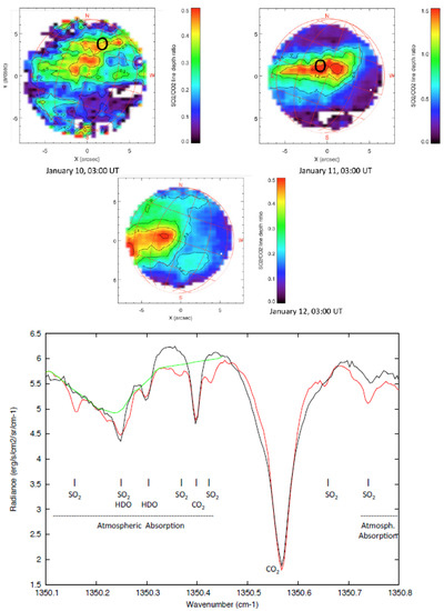
Figure 1.
Mapping of on Venus—Observations by TEXES. (Top panel) Map of the line depth ratio of / and its variability in time. From left to right: January 10; January 11; January 12 (2012). Values of the line depth ratio have a range of 0.0–0.5 for January 10 and 12; and 0.0–1.5 for January 11. The black circle indicates maximum absorption. (Bottom panel) TEXES observations of Venus, at approximately 1350.1–1350.8 (7.4 m). Red: spectrum corresponding to an area of the disk with a maximum abundance of . Black: spectrum corresponding to an area of the disk with a maximum of . Green: modeled telluric absorption. (image credits: Encrenaz et al. [23].

1.2. Mars
The next chemical species whose study we want to emphasize is methane on Mars. The first report on the detection of methane on Mars came out in 2004 by Krasnopolsky et al. [24]. A spectrum of Mars was recorded at the P-branch of the strongest band at 3.3 m with a resolving power of R = 180,000, using the Fourier Transform Spectrometer at the Canada–France–Hawaii Telescope (CFHT). An estimated amount of 10 ppb was retrieved for methane. In this study, the authors argued that methane production by hydrothermal, magmatic, cometary or interplanetary origin cannot account for the measured abundance. Therefore, they proposed the possibility of a biogenic origin.
There are reports of both positive and non-detections of methane on Mars by, respectively, observations by the MEx and ExoMars space probes [25,26]. The discrepancy between these has generated much debate [27,28,29,30,31,32].
1.3. The D/H Ratio
The measurement of elemental abundances and isotopic ratios is fundamental for understanding the origin and evolution of planets’ atmospheres [33]. One such ratio is the D/H ratio. In this work, we are interested in estimating the D/H ratio on Mars. To perform studies of the D/H ratio on Mars, space-based instruments and orbiting probes are used, avoiding the effect of terrestrial absorption [34,35].
The value of the D/H ratio constrains the origin and evolution of volatiles containing hydrogen in an atmosphere. Furthermore, the measurement of this ratio is necessary to trace the amount of water lost to space in an atmosphere. Other isotopic ratios such as /, / and / are important to constrain the solar nebula composition and the origin and evolution of volatiles in a planetary atmosphere. Furthermore, the measurement of the isotopic ratios of noble gases in an atmosphere are good indicators of atmospheric evolution [36].
The present work focuses on the determination of the D/H ratio since its value constrains the amount of water lost to space or to the subsurface through time. Since where there is water, there are habitability conditions [37], the measurement of this ratio allows to constrain the habitability conditions of Venus and Mars through time, in order to understand why the present Venus and Mars are so different from Earth despite being built from the same starting materials.
The measurement of the D/H ratio on Mars may provide valuable information. We can determine both a global and a local value for the D/H ratio which hold the answers to different questions [34]. Two of such questions are the following: (1) What was the abundance of the water reservoir on early Mars? (2) What are the current sinks and sources of water on Mars?
The determination of the global disk-integrated value of the D/H ratio is necessary to answer the first question, by comparison with the D/H ratio measured in clays at the Martian surface and of ancient SNC meteorites [38,39,40]. Hence, the measurement of this ratio is important in the study of the abundance of water on Mars through time. The determination of the local value of the D/H ratio, i.e., varying with altitude, season and location is necessary to answer the second question [41,42,43,44,45]. The variation of this value is determined by fractionation processes, such as different escape rates associated with the deuterium and hydrogen atoms [46]. The hydrogen atoms escape more easily than the deuterium atoms, since the former are lighter. Different condensation/sublimation points of water and HDO depend on local temperature, saturation levels and aerosol column abundances [35].
The ExoMars mission is currently measuring the D/H ratio on Mars to inform us about the processes that contributed and might still contribute to atmospheric depletion on Mars [35]. On Venus, future missions such as the ESA’s EnVision mission intend to contribute to a better understanding of the atmospheric evolution of Venus, which seems to have lost most of its water to space, given its high D/H ratio [47,48].
ExoMars solar occultation observations, by the Nadir and Occultation for Mars Discovery (NOMAD) instrument, centered at 3.6 m (2730 ) (HDO) and at 3.3 m (3025 ) (), show that the water vapor abundance in the middle atmosphere (40–100 km) increases up to two orders of magnitude during a Global Dust Storm (GDS), reaching altitudes of 100 km [35]. With regard to the D/H ratio, the main results of the latter study were: (1) the D/H ratio is ∼6 VSMOW (Vienna Standard Ocean Water, corresponding to D/H ∼) in the lower atmosphere; (2) the D/H ratio decreases with altitude and (3) the D/H ratio is low (2–4 VSMOW) at high/low latitudes and close to the equinox where the abundance is low [35]. The decrease in D/H with altitude can be attributed to Rayleigh fractionation, due to atmospheric dynamics, cloud formation and atmospheric microphysics [49], as for the case of Earth [50]. The D/H ratio measurements during the equinox can be explained by the low water abundance measured in this period, where a compacted hygropause leads to the measured low D/H ratio. Nevertheless, the measured D/H ratios at equinox are inconclusive since water is confined to low-altitude layers of the atmosphere, where long-atmospheric path lengths prevent observations of HDO with enough sensitivity due to aerosol extinction [35]. Therefore, further dedicated observations are needed to determine with certainty the source of the low D/H ratios measured at equinox.
Three processes that can contribute to the escape of water on Mars through photolysis of water in the upper atmosphere are global dust storms, the regional dust storms and the summer seasons [35].
The value of the D/H ratio of Jupiter and Saturn inform us about the conditions of formation of these planets. If these planets formed from the accretion of gas from the protosolar nebula, then the measured D/H ratio should be similar to the measured protosolar D/H ratio [33].
2. Observations
In this Section, we present a brief review of the results of recent studies concerning the detection and the measurement of abundances of sulphur dioxide and phosphine on Venus, methane and the D/H ratio on Mars and ammonia, phosphine, methane and deuterated methane on Jupiter.
2.1. Venus
Observations of the lower mesosphere were performed with TEXES at the Infrared Telescope Facility (IRTF) at approximately 7.4 m [23], corresponding to an altitude of km (see Figure 1). TEXES is an infrared imaging spectrometer operating between 5 and 25 m which combines high spatial (about 1.5 arcsec) and spectral (R = 80,000) resolution. These observations show a spatio-temporal variation of sulphur dioxide. This gas is most concentrated in patches and varies within a timescale of days.
Encrenaz et al. [22], through observations in the infrared using TEXES (see Figure 2), at 951–956 (10.46 m–10.52 m), did not detect phosphine absorption lines, but instead proposed an upper limit of 5 ppb for its abundance, close to the value proposed by Greaves et al. [19], corresponding to 7 ppb.
2.2. Mars
An independent confirmation of the positive detection of methane on Mars was performed by spot-tracking nadir observations of the Gale Crater by the Planetary Fourier Spectrometer (PFS) instrument on MEx, taken in the IR (3.3 m), on June 2013 [25] (see Figure 3, top panel). This mode allows the acquisition of several hundred spectra within a very short time (tens of minutes), increasing the SNR of the observations. Through the use of improved observational geometry and data treatment and analysis, a methane absorption feature at approximately 3018 was detected, corresponding to an estimated abundance of 15.5 ppb. This detection was performed one day after the in situ detection of methane by Curiosity [51], also near Gale Crater. This study suggests that methane is released by the surface, in regions where faults meet shallow ice formations, and this release is characterized by being short and small [25].

Figure 3.
Positive and non-detection of methane on Mars by the MEx and ExoMars space probes, respectively. (Top panel) Measured integrated radiance spectrum, in cgs units (), taken by the PFS instrument on MEx, showing a methane absorption feature at approximately 3018 , by summing hundreds of spectra (image credits: Giuranna et al. [25]). (Bottom panel) Transmittance spectrum measured by the ExoMars TGO NOMAD SO instrument during the dust storm. An upper limit of 0.05 ppb of methane was estimated [26]. Data—black; blue—synthetic model with 1 ppm of and no methane; yellow—synthetic model with 0.5 ppb of methane; red—synthetic model with 0.05 ppb of methane (image credits: Korablev et al. [26]).
A recent example of the non-detection of methane on Mars follows from the highly sensitive measurements of the Martian atmosphere by the ExoMars Trace Gas Orbiter (TGO) Nadir and Occultation for Mars Discovery (NOMAD) and Atmospheric Chemistry Suite (ACS) instruments from April–August 2018 observations [26] (see Figure 3, bottom panel) in solar occultation geometry. These observations are best suited for the detection of minor atmospheric species due to two main factors: (1) the Sun’s brightness increases the SNR of the spectra; and (2) becomes a ten times longer atmospheric optical path in relation to nadir geometry (looking to the surface). The spectral range of the instruments covers the 3.3 m spectral range, where the strongest fundamental absorption bands of methane are located [52]. Observations were performed before the great dust storm of August 2018 by the ACS instrument and by the NOMAD instrument. For a combination of different latitudes of measurements in both hemispheres, methane was generally not detected at high latitudes. Instead, an upper limit for its abundance was derived to be approximately 0.05 ppbv, nearly two orders of magnitude lower than in previous detections [25,53]. The optimal altitude to search for methane is located at approximately 5–25 km, according to Korablev et al. [26], corresponding to an equilibrium between two effects: (1) the increase in sensitivity when the line of sight of the instrument samples closer to the surface; and (2) the decrease in sensitivity closer to the surface due to the presence of dust and clouds. The authors claimed that a possible explanation for the mismatch between this study and the one from Giuranna et al. [25] is the existence of an unknown process that rapidly removes methane from the lower atmosphere before it spreads globally on Mars.
It is important to avoid the effect of terrestrial transmittance when observing Mars. One instrument that minimizes this effect is the Echelon Cross Echelle Spectrograph (EXES) onboard the Statospheric Observatory for Infrared Astronomy (SOFIA). EXES was used to observe , HDO and transitions at 1383–1391 (7.19–7.23 m), for April 2017 and March 2016 observations [34] (see Figure 4).
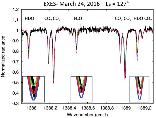
Figure 4.
Determination of the D/H ratio on Mars—observations by EXES, onboard SOFIA, at approximately 1383–1391 . Spectrum of the northern hemisphere of Mars in March 2016. The stronger lines are from and there are several weaker HDO and lines. In Section 4, the HDO line at 1388 , the HDO line at 1389.1 and the line at 1388.5 were modeled for different and HDO abundances to estimate the D/H ratio. Green: = 250 ppm, HDO = 400 ppb; red: = 375 ppm, HDO = 550 ppb; blue: = 500 ppm, HDO = 700 ppb. (image credits: Encrenaz et al. [34]).
2.3. Jupiter
Using the short wavelength spectrometer (SWS) and the long wavelength spectrometer (LWS) instruments onboard the Infrared Space Observatory (ISO) mission, observations of Jupiter and Saturn at 2.3–180 m were analyzed with a resolving power of R = 150–30,000 [54]. The main conclusions of the latter study were: (1) detection of water vapor in the deep troposphere of Saturn; (2) the detection of new hydrocarbons in Saturn’s stratosphere (, , , ); (3) the detection of water vapor and carbon dioxide in the stratospheres of Jupiter and Saturn; and (4) the new determination of the D/H ratio using the detection of new HD rotational lines [54].
We want to focus on the results of the analysis of the 6 m–14 m spectral region on Jupiter observations (see Figure 5). This wavelength interval is sounding a region just below and above the tropopause. Therefore, the spectrum has both emission ( at 7.7 m) and absorption lines (, , ). The continuum in this regime is due to the hydrogen–helium pressure-induced spectrum and to the cloud. Abundances of and were assumed for and , respectively [54].
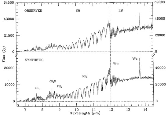
Figure 5.
Mean Jupiter spectrum recorded by the SWS instrument on ISO, at 6–14 m. The main molecular features of the spectrum are identified (image credits: Encrenaz et al. [54]).
3. Methods
In this section, we describe the tool used to perform the simulations and the methods used to perform the detection and determination of the abundances of minor chemical species. All simulations in this work were performed by the Planetary Spectrum Generator.
3.1. The Planetary Spectrum Generator
The Planetary Spectrum Generator (PSG) [55] is an online radiative transfer suite for the simulation of the spectrum of planets, exoplanets, comets and other small bodies. The synthesized spectra can cover a broad range of wavelengths, from the radio to the UV. It combines radiative transfer modeling, spectroscopic databases (for example, HITRAN [56]) and planetary ephemeris databases (Horizons System—JPL Solar System Dynamics—NASA) to perform spectra simulations. The computation of the high-resolution spectra uses line-by-line calculations and uses the correlated-k approach for moderate resolutions.
PSG can be used to do a fit between observations and modeled spectrum in order to determine, for example, the abundance of atmospheric species and the temperature and altitude of the atmospheric level that the observations are sounding, among other parameters [55]. To perform the retrieval, PSG employs the optimal estimation method ([57]). Moreover, PSG can help plan observations, interpret ground-based and space-based data and in the calibration of instrumental effects, such as the instrument’s gain issues, offset issues, fringe issues and incomplete stellar subtraction.
PSG can be used in a web-interface, or run remotely by sending instructions to produce spectra to the online server.
The parameters of the modeled spectrum are defined on a configuration file which is the main input file that can be downloaded from the web interface or created by the user. The parameters are divided in three main fields: atmospheric parameters; object and geometry parameters; and instrumental parameters. To see a complete description of these parameters, see Villanueva et al. [55].
The resulting output of the simulation is a spectrum (the units depend on the simulation), the transmittance of the atmospheric components included in our model atmosphere and the noise components of the observations in the selected wavelength range. All these outputs can be downloaded from the web-interface page or downloaded through terminal instructions to the server.
3.2. Atmospheric Models
For Venus, we used two different atmospheric models: the VIRA-2 model and the LMD-VGCM model. The LMD-VGCM model stands for the Laboratoire de Météorologie Dynamic Venus Global Circulation Model [58,59]. It was inspired by the GCMs developed for Earth and Mars. It is the only existing ground-to-thermosphere Venus GCM. The simulation of the atmosphere at 90–150 km includes processes such as IR heating by , IR 15 m cooling, extreme UV heating and a photochemical model. The simulated thermal structure is consistent with Venus Express data. The VIRA-2 model stands for Venus International Reference Atmosphere [60]. VIRA is an empirical model that relies on data from several missions from the 1970s and 1980s such as Venera, Pioneer Venus Orbiter, Vega and Magellan space probes and most recently Venus Express and Akatsuki.
For Mars, we used the Mars Climate Database (MCD) as atmospheric input for PSG to simulate the MEx and ExoMars observations [61,62] model.
For Jupiter, the atmospheric model used was a non-linear optimal estimator for multivariate spectral analysis (NEMESIS) composite infrared spectrometer (CIRS) with a Cassini space probe template. NEMESIS is a state-of-the-art radiative transfer suite ([63]).
3.3. Detection of Minor Species
To perform the detection of minor chemical species, we identified the presence of molecular absorption/emission in our simulated spectra. This was achieved by performing, for each species, several simulations using different scalings of the template vertical abundance profile of the respective species, i.e., my multiplying the template (initial) profile by a scalar bigger or smaller than 1. This method allows one to distinguish between the molecular spectral features originating from different molecules (see Figure 6 and Figure 10 for the detection of minor species on Venus, Figure 13 for the detection of minor species on Mars and Figure 18 for the detection of minor species on Jupiter). An absorption feature is associated with a species if an increased abundance of such species in our model results in an increase in the depth of that absorption feature. This absorption feature can be an absorption line or an absorption band (see Section 4).
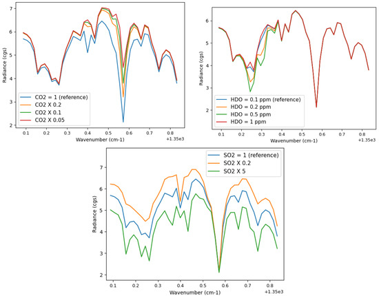
Figure 6.
Exploration of the effect of the variation of the abundance of , HDO and of the model on the Venusian spectrum, at 1350.1–1350.8 , for R = 80,000. (Top row, left panel) A decrease in the abundance of in the model results in a decrease in the resulting radiance; (Top row, right panel) An increase in the abundance of HDO in the model results in an increase in the depth of two lines. This suggests that these lines have a contribution from HDO absorption; (Bottom row) An increase in the abundance of in the model results in the decrease in the resulting radiance and of the depth of some lines, which suggests that those are lines. The error of the simulations is approximately 0.1%. See Table 1 for a list of the lines.
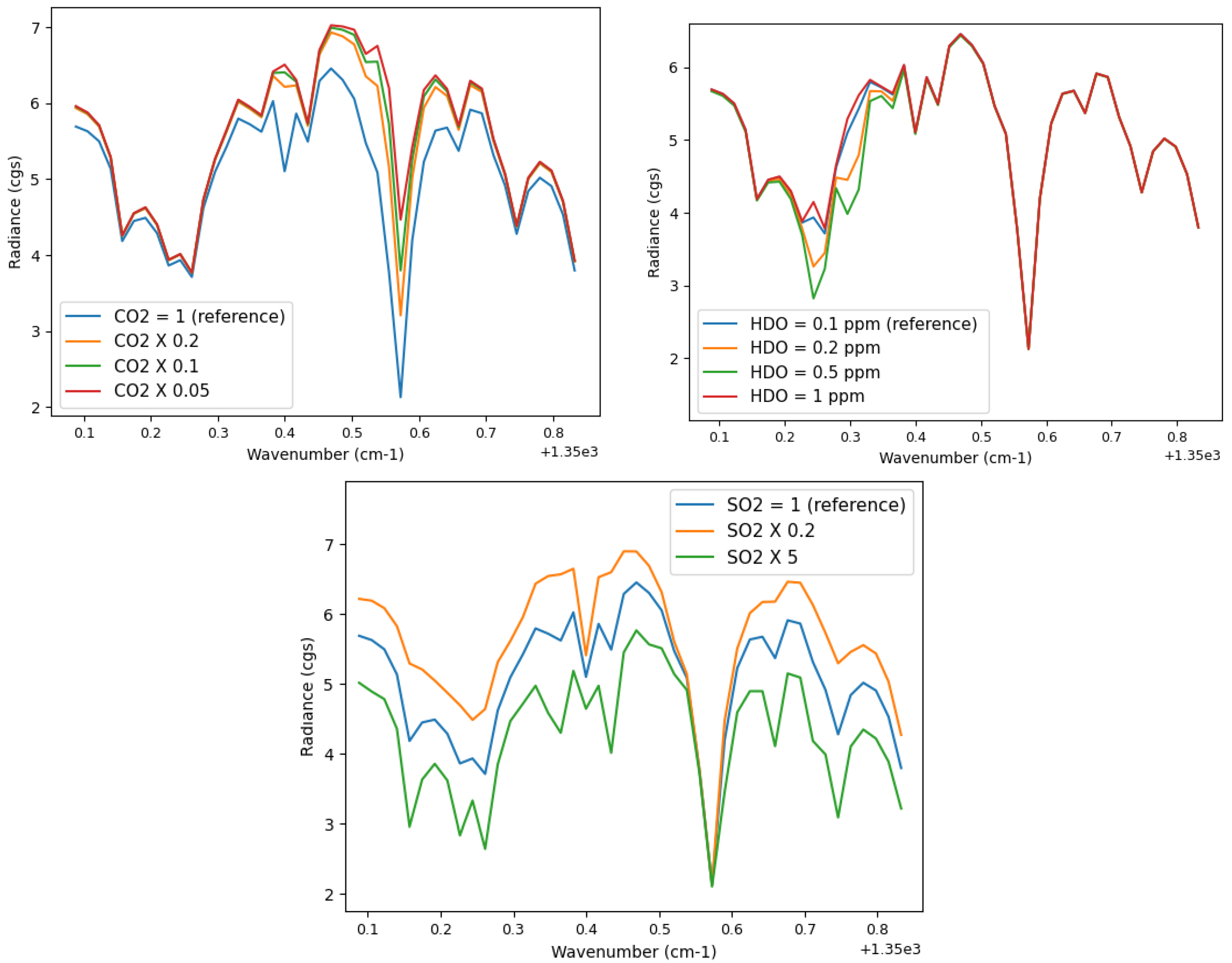

Table 1.
Sulphur dioxide on Venus—line identification: 1350–1350.8 . The position of the lines agrees with the values from HITRAN [56,64,65,66,67,68]. For line 6, there is more than one possible molecular candidate for the spectral feature. The uncertainty of the line positions in the simulation derive from the resolution of the simulation (∼0.017 ).
| Line () | PSG | PSG Doppler Corrected | HITRAN |
|---|---|---|---|
| 1 | 1350.159 ± 0.009 | 1350.113 ± 0.009 | —1350.1134 ± 0.0001 |
| 2 | 1350.226 ± 0.009 | 1350.180 ± 0.009 | —1350.1780 ± 0.0001 |
| 3 | 1350.260 ± 0.009 | 1350.214 ± 0.009 | —1350.2138 ± 0.0001 |
| 4 | 1350.310 ± 0.009 | 1350.264 ± 0.009 | HDO—1350.25853 ± 0.00001 |
| 5 | 1350.361 ± 0.009 | 1350.315 ± 0.009 | —1350.3156 ± 0.0001 |
| 6 | 1350.395 ± 0.009 | 1350.349 ± 0.009 | —1350.3519 ± 0.0001 |
| —1350.3470 ± 0.0001 | |||
| 7 | 1350.429 ± 0.009 | 1350.383 ± 0.009 | —1350.3830 ± 0.0001 |
| 8 | 1350.564 ± 0.009 | 1350.518 ± 0.009 | —1350.5250 ± 0.0001 |
| —1350.5100 ± 0.0001 | |||
| 9 | 1350.648 ± 0.009 | 1350.602 ± 0.009 | —1350.6020 ± 0.0001 |
| 10 | 1350.732 ± 0.009 | 1350.686 ± 0.009 | —1350.6867 ± 0.0001 |
3.4. Determination of the Abundances
For the determination of the abundance of the minor species in this work, we used two different methods: the line depth ratio (ldr) method, developed by Encrenaz et al. [23] and the retrieval method, based on the Optimal Estimation [57] method. The line depth ratio consists of rationing the line depths of weak neighboring transitions of minor species with respect to . As a result, this cancels, in first order, the effects associated with geometry, calibration and atmospheric parameters [69]. This is valid when assuming that the line depth ratios vary linearly with the mixing ratios of the species. This works for line depths weaker than approximately 10% [69]. The retrieval problem is defined in terms of an input (data), a series of unknown parameters to retrieve and a model that represents the physics of the atmosphere and surface of the planetary target. The goal of the retrieval is to find the parameters that minimize the difference between the data and the model, i.e., to minimize a particular cost function. The principle of optimal estimation is to link the data space and the parameter space by an analytical equation that comes from the solution to the minimization of the cost function. The cost-function chosen by PSG is the (chi-squared) of the spectral residues:
where R is a vector with the radiance values of the observations, r is a vector with the simulated radiances of our model, represents a vector with the uncertainties of the observations and N is the number of spectral points of the observations [55].
4. Results
4.1. Sulphur Dioxide on Venus
To identify , and HDO lines in the simulation, we varied the abundance of these species in the model and studied how the resulting radiance varied (see Figure 6), fixing all other parameters of the simulation. The spectra are Doppler shifted by +0.045 , corresponding to a relative velocity between Earth and Venus of approximately −10 km s.
To check whether the detected lines in the simulation were true detections, we did a comparison between the position of the lines in the simulations, corrected for the Doppler shift due to the relative velocity between Earth and Venus at the time of the observations, with the positions extracted from HITRAN [56,64,65,66,67,68] (Table 1).
The line identification is clear on Figure 7 together with the comparison of the two simulations with data.
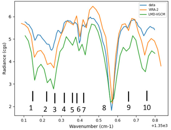
Figure 7.
Comparison between simulations and TEXES data ([23]). Two simulations are compared to the data (blue). The VIRA-2 model (orange) has a higher radiance than the LMD-VGCM model (green) and weaker and narrower lines compared with the LMD-VGCM model. The uncertainty of the datapoints of the observations is approximately 5%. The error of the simulations is approximately 0.1%. The absorption lines were numbered and can be consulted in Table 1. cgs units= erg s cm sr; VIRA-2 model: [60]; LMD-VGCM model: [58,59].
The line depth ratio method (ldr) consists of measuring the line depth ratio between a weak line and a strong line (highlighted in Figure 8), for various abundances of . If this variation is linear, then comparing with the / line ratio of the observations, we can infer the abundance of . The value of the / ratio of the observations is approximately 0.25. The retrieval works through the use of a retrieval module included in PSG. It adjusts the entire vertical profile [60], using a scaling factor, to obtain a best match to the observations. The result of the retrieval is in Figure 9.
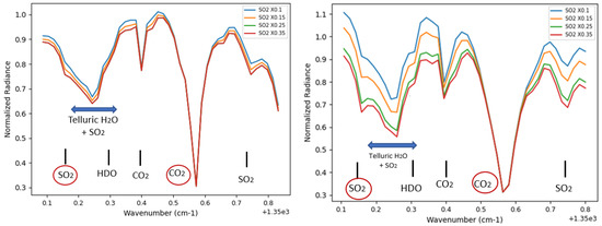
Figure 8.
Effect of the variation of abundance on the resulting radiance—ldr method on Venus. Small variations of the abundance of were used since the depth of the corresponding lines are sensitive to small variations. (Left panel) VIRA-2 model. Four different abundances of were used, represented by a different scaling factor (for example, = ×0.1 corresponds to a model where the standard abundance of in VIRA-2 was multiplied by 0.1). The red circles highlight the and lines used to calculate the line depth ratio. The ldr(/) scales linearly with the abundance of . (Right panel) LMD-VGCM model. Four different abundances of were used. The ldr(/) scales linearly with the abundance of . The error of the simulations is approximately 0.1%.
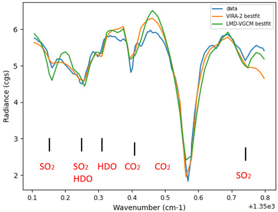
Figure 9.
Best fits obtained for TEXES data. The VIRA-2 model provides the simulation with the best match to data. The fitted parameters were the vertical abundance profile and the telluric water absorption. The telluric water absorption is at 1350.1–1350.3 . The line positions identified corresponds to those of HITRAN [56] (see Table 1) and matches the identification made by Encrenaz et al. [23]. The uncertainty of the datapoints of the observations is approximately 5%. The error of the simulations is approximately 0.1%. Blue—data; green—LMD-VGCM model; orange—VIRA-2 model.
The parameters fitted by the optimal estimation are a scalar of the profile and the telluric water column affecting the observations. The first parameter fitted was the strong absorption line. As seen in Figure 9, the VIRA-2 model provides a better fit to the line than the LMD-VGCM model. Then, we fitted it for the telluric water absorption. Again, we see that the VIRA-2 model presents a better fit to the telluric transmittance than the LMD-VGCM model. Finally, we fitted it for the abundance. The VIRA-2 model provides the best-fit to the observations at 1350–1350.7 , where it has a lower , since it better fits the line at 1350.6 and the telluric transmittance at 1350.1–1350.3 , although the LMD-VGCM model provides a better fit to the line at 1350.73 . For the entire wavenumber interval, the VIRA-2 model has ∼6, while the LMD-VGCM model has ∼1, where N is the number of spectral points of the simulation minus the number of degrees of freedom of the retrieval.
The estimated abundances obtained for are shown in Table 2.
Table 2.
Estimated abundance of for a combination of different models and methods. The lower value of the VIRA-2 model using the line depth ratio method corresponds to a situation where the abundance of is derived without including telluric absorption in the simulation. The range of abundance of derived from observations comes from spatial and temporal variability.
The value estimated for the abundance of using the line depth ratio method, within an order of magnitude, agrees with the literature (see Table 2). The discrepancy from the value of the literature [23] derived from the retrieval method is lower than the discrepancy derived from the line depth ratio method. The result with the lowest discrepancy corresponds to the abundance obtained using the VIRA-2 model and the line depth ratio method. The result with the highest discrepancy corresponds to the abundance obtained using the LMD-VGCM model and the line depth ratio method. In order to improve the determination of the abundance for the specific case above and to complement the current estimates, we will perform simulations, in a future study, to determine the abundance using the line depth ratio method; however, instead of using the line at 1350.159 , we will use the line at 1350.732 , since this line has no contamination from telluric water absorption.
The first step of the retrieval procedure was to fit the strong line, at approximately 1350.6 , the second was to fit the water absorption at 1350.2–1350.3 , and finally to fit the absorption lines.
The overall uncertainty of the retrieval method is approximately 4%, when using the VIRA-2 model and approximately 9% when using the LMD-VGCM model and depends on the uncertainty of the radiance measured in the observations, which was assumed to be 5% by the PSG retrieval module.
The uncertainty in the line depth ratio method is mainly due to: (1) difficulties in the definition of the continuum in the observations due to the modeling of the water absorption, which will introduce an uncertainty in the measurement of the depth of the lines; (2) the atmospheric model used, and in particular, uncertainties in the model in the definition of the vertical profile, since there is evidence in the literature for variations of a factor of 5–10 in the abundance of this species [23].
The uncertainty derived from the definition of the continuum can be estimated by performing simulations without including telluric transmittance and comparing with the ones that include telluric transmittance. The abundance obtained for without including telluric transmittance is approximately 100 ppb using the line depth ratio method. Therefore, we conclude that the definition of the telluric transmission can induce an uncertainty of approximately 35%, for the VIRA-2 model simulations (with a derived abundance of of approximately 154 ppb, including telluric transmittance). The uncertainty accounting for the possible variability of the abundance at the cloud top can be represented by the difference in the abundance between the VIRA-2 and the LMD-VGCM models. This uncertainty can be accounted for by joining the two intervals of abundance derived for (100–154 ppb for the VIRA-2 model and 20–43 ppb for the LMD-VGCM model). However, the abundance of derived from the LMD-VGCM model, with the line depth ratio method, is below the interval estimated by Encrenaz et al. [23] (approximately 50–175 ppb). This discrepancy has not been understood to date. Several factors can explain this discrepancy. For example, the VIRA-2 and LMD-VGCM models have different temperatures at the cloud top level, resulting in different continuum levels and different depths for the absorption lines. Looking at the line at 955.4 in Figure 9, we see that the VIRA-2 model has a better fit to the line than the LMD-VGCM model. Therefore, there will be an associated discrepancy when determining the abundance. Another factor that can contribute to the highlighted discrepancy is the different and vertical abundance profiles of the VIRA-2 and LMD-VGCM models.
All the steps performed to determine the abundance of are of paramount importance to help in the search for phosphine on Venus, since telluric lines and lines overlap with phosphine lines throughout the IR and sub-millimeter/microwave wavelength range.
4.2. Phosphine on Venus
To identify lines, we performed the simulations in Figure 10, with a resolving power of R = 80,000, between 955.15 and 955.4 , in order to reproduce the observations found by Encrenaz et al. [22]. We simulated the telluric transmittance using PSG (only water lines). The spectrum was Doppler shifted by approximately +0.035 , corresponding to a relative velocity between Venus and Earth at the time of the observations of approximately −11 km s. We performed simulations for different phosphine abundances: 5 ppb, 7 ppb and 10 ppb. It is very difficult to spot the phosphine absorption line at 955.26 due to a strong telluric water band at 955.2–955.3 .
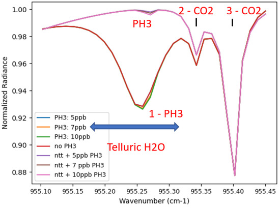
Figure 10.
Exploration of the effect on the Venusian spectrum of the variation of abundance of , between 955.15 (10.470 m) and 955.4 (10.467 m), for a resolving power of R = 80,000. The simulations were normalized by the maximum value of radiance in each simulation as a first approximation. Telluric water absorption dominates the region of the spectrum where the phosphine absorption line should be present, namely at 955.15–955.35 . The simulations include three different phosphine abundances—5 ppb, 7 ppb and 10 ppb—for two different situations, namely telluric absorption and removing telluric absorption (ntt). Without telluric absorption, it is much easier to identify the phosphine absorption line than it is when including telluric absorption. Absorption lines are numbered (see Table 3). The error of the simulations is approximately 0.1%.
We identified the absorption lines in the spectrum and compared them with the transition positions from HITRAN [56,67,70] (Table 3).
Table 3.
Phosphine on Venus—line identification: 955.15–955.4 . See Figure 10. The position of the lines agrees with the positions reported in HITRAN [56,67,70]. The uncertainty of the line positions in the simulation derive from the resolution of the simulation (∼0.012 ).
In Figure 11, there is a comparison between the simulations and the data. There is a discrepancy of a maximum of a factor of 2 between the data and the simulations.
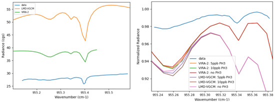
Figure 11.
(Left panel) Comparison between the simulation and observations (blue) by Encrenaz et al. [22], using the VIRA-2 model (green) ([60]) and the LMD-VGCM model (orange) [58,59] as inputs for PSG. The LMD-VGCM model presents the higher values of radiance. Moreover, it has deeper and broader lines than the VIRA-2 model and data. Both simulations have broader and deeper lines than the data, as well as stronger water absorption at approximately 955.2–955.3 . cgs units = erg s cm sr; (Right panel) Zoom of the left plot at approximately 955.24–955.38 in normalized radiance units. The effect of different abundances of phosphine, 5 ppb and 10 ppb, in the simulations, are shown. The normalized radiance of our simulation, at approximately 955.25 , is approximately 4% and 5% deeper than the normalized radiance of the data for, respectively, the VIRA-2 model and the LMD-VGCM model, when considering the simulations with 5 ppb of . The uncertainty of the datapoints of the observations is approximately 5%. The error of the simulations is approximately 0.1%.
Using the retrieval module of PSG, we conclude that the best fit is achieved by the VIRA-2 model, with ∼0.1, compared with ∼0.6 for the LMD-VGCM model (see Figure 12).
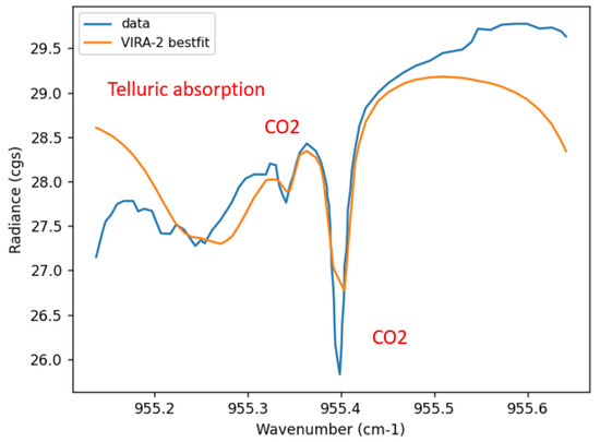
Figure 12.
Best fit models — Phosphine. Orange—VIRA-2 best-fit. Blue—data. The main absorption features are identified. Below 955.2 and above 955.4 , the simulation deviates from the data. The uncertainty of the datapoints of the observations is approximately 5%. The error of the simulations is approximately 0.1%.
The absorption line could not be detected either in the simulation or in the observations.
Looking at Figure 11, we can see that there is a discrepancy below a factor of approximately 2 between the data and the simulations. The VIRA-2 model in particular has a higher radiance than the data, up to approximately 36% (at 955.2 ), and a lower radiance with respect to the LMD-VGCM model, up to approximately 28% lower (at 955.2 ). The LMD-VGCM model has a lower temperature than the VIRA-2 model in the pressure region of interest. Moreover, it is important to notice that the lines at approximately 955.4 and 955.34 of both models are broader than those from the data. For the line at 955.4 , the corresponding depths are, respectively, for the data, the VIRA-2 and the LMD-VGCM simulations, as follows: ∼0.13, ∼0.11, ∼0.24. In detail, we see that the VIRA-2 model has narrower lines that the LMD-VGCM model.
Regarding the telluric water absorption in both models, it is broader and stronger than in the data. This discrepancy in the telluric water absorption was solved when doing the fit of telluric transmittance using the PSG retrieval module.
The depth of the phosphine line can be estimated based on the difference between the depth at the position of the line using simulations with phosphine included in the model and simulations without phosphine included in the model. For example, for 10 ppb of , the depth of the line is approximately 0.002, in comparison with 0.07 for the depth at the same wavenumber (approximately 955.26 ) without phosphine. Thus, the contribution of phosphine is approximately 3% of the contribution of the telluric absorption to the depth at 955.26 . When the telluric transmission is removed in our simulations, the phosphine absorption line appears clearly visible; however, it is still very weak (see Figure 10).
4.3. Methane on Mars
The goal is to simulate both a positive and non-detection of methane on Mars. The positive detection was that which was carried out by the PFS instrument on MEx [25]. The non-detection is based on the ExoMars NOMAD/ACS TGO instruments’ observations [26]. The spectra simulations are shown in Figure 13.
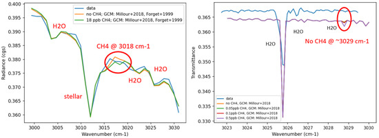
Figure 13.
Comparison between best-fit simulations and data. (Left panel) Comparison between the simulation and MEx data [25]. Blue line: data. Orange line: MCD [61,62] with no methane. Green line: MCD with 18 ppb of methane. The red circle highlights the region where the methane absorption feature is present, both in the data and in the orange line. We chose 18 ppb of methane as a first educated guess for the abundance of methane following Giuranna et al. [25]. The simulation with no methane has a ∼4.8 and the simulation with 18 ppb of methane has ∼5.4. One stellar line and several water absorption features are identified (see Table 4 for the position of the absorption features); (Right panel) Comparison between the simulation and ExoMars data ([51]), at 3023–3030 . absorption features are identified. Several abundances of methane were simulated, namely 0.05 ppb (green line), 0.1 ppb (red line) and 0.5 ppb (purple line). The upper limit derived by observations was 0.05 ppb [26]. For an abundance of 0.5 ppb, a methane opacity source was identified in the simulation and therefore should have been detectable by the ExoMars space probe. We used 0.5 ppb of methane abundance as a first educated guess following Korablev et al. [26].
Following the same procedure as for the case of Venus, we varied the abundance of and of the Martian reference spectrum, fixing all other parameters of the simulation, in order to identify the absorption features of these species (see Figure 14, Table 4).
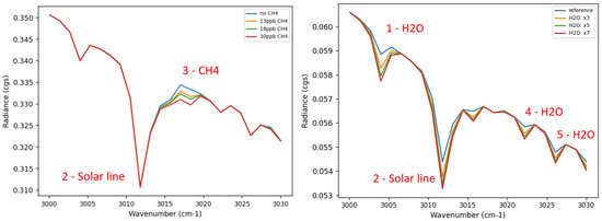
Figure 14.
Identification of and absorption features in MEx simulations—Mars. (Left panel) Effect of the variation of methane abundance in the model on the resulting radiance for = 0 ppb (blue), 13 ppb (orange), 18 ppb (green) and 30 ppb (red). A methane absorption feature was identified. (Right panel) Effect of the variation of in the model in the resulting radiance, for = 1 (blue, standard abundance of in the model), = 3 (orange), = 5 (green) and = 7 (red). Three absorption features were identified. The position of the absorption features agrees with the positions in HITRAN [56] (see Table 4).
Table 4.
Methane on Mars, MEx observations—comparison between the position of the absorption feature center in the simulation and the position of the strongest absorption line from the same species from HITRAN in a wavenumber range centered in the position of the absorption feature in the simulation. The position of the absorption features agrees with the positions from HITRAN ([56]).
The first step in fitting for the MEx data was to fit the solar line at approximately 3012 . The second step was to fit the water lines, by adjusting the abundance of water in the model by a scaling factor. The simulation with no methane (orange line) has a ∼4.8 and the simulation with 18 ppb of methane (green line) has ∼5.4. This is an a priori value, i.e., a first educated guess of the abundance following Giuranna et al. [25]. At approximately 3015–3025 , a correction function was applied to the observations by Giuranna et al. [25], due to the instrument line shape of the PFS. This correction, at present, was not applied to the simulation, since we do not know what the correction function is. In future work, we will determine the correction function we have to apply to the simulation in order to constrain the methane abundance using PSG.
The first step in fitting for ExoMars data was to adjust the level of the continuum of the simulation with the one from the observations. This was achieved by changing the abundance of dust and ice in the model, by multiplying or dividing the vertical abundance profiles by a scaling factor, as well as by changing the altitude of the line of sight of the solar occultation in the model. Ice clouds were removed from the model, the dust abundance was set equal to the standard profile from the MCD [61,62] and the height of the occultation was set to 8.6 km, close to the altitude of the observations, 5.9–8.0 km.
Methane was not detected in the ExoMars data around 3029 . However, our simulations show that a methane abundance of 0.5 ppb should have been detectable by the ExoMars space probe. This is an a priori value, i.e., a first educated guess of the abundance following Korablev et al. [26]. The methane opacity source is located at approximately 3028.8 ± 0.1 . Within this interval, there are 34 molecular transitions in HITRAN of interest, due to molecules such as , , and [56], where most transitions are due to . The strongest methane line is at 3028.7522600 with an intensity of ∼/(molecule ). The strongest line is at 3028.7202 with an intensity of ∼/(molecule ). The strongest line is at 3028.9079 with an intensity of ∼/(molecule ). This highly suggests that the molecular absorption feature centered at 3028.8 is due to methane. To confirm this, nevertheless, we calculated the line to the continuum ratio for and at approximately 3028–3029 . For , for example, this is the ratio between the transmittance spectrum when has the standard abundance [61,62] and the transmittance spectrum when has an abundance set to 0. From this ratio, we verified that the molecular absorption feature centered at 3028.8 , for an abundance of 0.5 ppb of , is due to an overlap of several absorption lines with a absorption line.
We can see that we have a case of positive detection and a case of non-detection of methane. This discrepancy might be explained by the possibility of the methane abundance in the Martian atmosphere having a spatial and temporal variation. However, it is not clear why the Martian atmosphere would allow such a differentiation according to the most recent photochemistry and global circulation models [71,72].
A discussion of some possible reasons that may explain both the positive and non-detections of methane is explored in Section 5.
4.4. Determination of the D/H Ratio—Mars
Observations from Encrenaz et al. [34] were simulated at 1388–1389.2 without terrestrial absorption applied in PSG. The atmospheric model used was the MCD [61,62]. The simulation was compared with the data in Figure 15.
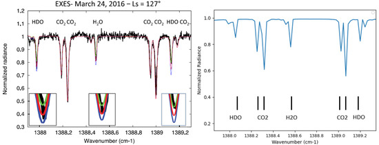
Figure 15.
Comparison between the simulation and EXES data at 1388–1389.2 ([34]). (Left panel) EXES data, at 1388–1389.2 , with the corresponding line identification. The line identification is identical in both figures. Green: = 250 ppm. HDO = 400 ppb. Red: = 375 ppm. HDO = 550 ppb. Blue: = 500 ppm. HDO = 700 ppb. (Right panel) Normalized radiance simulation with the corresponding line identification. There is a discrepancy in the depth of the and HDO lines between simulation and observations. This means that the simulated opacities for HDO and transitions assume abundances that disagree with the abundances derived by Encrenaz et al. [34].
First, we measured the depth of the weak line at approximately 1388.6 , the weak HDO line at 1388 and the weak line at 1367.97 . Then, considering a fixed abundance of 450 ppb of HDO, we tried different abundances, such as 100 ppm, 200 ppm, 300 ppm, 450 ppm and 500 ppm and performed the corresponding simulations. After this, we fixed the abundance of at 318 ppm, and performed simulations for the following abundances of HDO: 300 ppb, 350 ppb, 400 ppb, 500 ppb, 550 ppb and 600 ppb (see Figure 16). For each of these combinations of abundances, we measured two line depth ratios: ldr(HDO/) and ldr(/). We studied their variations for the different combinations of abundances. We obtained the following linear equations: ldr (HDO/) = 0.0055 vmr (HDO) + 0.9732 and ldr () = 0.009 vmr () + 0.3114.
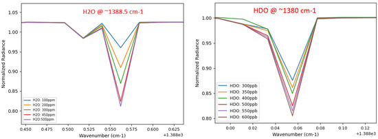
Figure 16.
Variation of the abundances of HDO and in EXES simulations. The depth of the lines linearly increases with their abundances. (Left panel) HDO = 450 ppb for = 100 ppm, 200 ppm, 300 ppm, 450 ppm and 500 ppm; (Right panel) = 318 ppm, for HDO = 300 ppb, 350 ppb, 400 ppb, 500 ppb, 550 ppb and 600 ppb.
Finally, we substituted the value of ldr(HDO/) and ldr(/) obtained in the data in the latter expressions to estimate the abundance of and HDO. For the data, we have ldr(HDO /)∼4.17, ldr (/)∼3.17.
The estimated abundances of HDO and were 581 ppb and 318 ppm, respectively. The values obtained by Encrenaz et al. [34] were HDO = 303–397 ppb and = 253–307 ppm.
The calculation of the D/H ratio gives D/H∼5.9 D/H (Earth), in comparison with D/H = 3.4–4.8 D/H (Earth) ([34]).
The uncertainty associated with the estimation of the D/H ratio may have multiples sources including (1) the definition of the continuum level and therefore the measurement of the depth of the lines of , HDO and ; (2) the presence of telluric absorption; (3) a possible deviation from linearity between the line depth ratio and the abundances; and (4) different pairs of / and HDO/ lines may give different estimations of the abundances and therefore of the D/H ratio. We used one HDO line and one line to estimate the D/H ratio. To improve the estimate, one way forward would be to repeat this method for several and HDO line pairs, located at approximately 1382–1391 (7.2 m). The quantitative contribution from each of these possible uncertainty sources is being evaluated. Furthermore, these identified uncertainties sources do not preclude the existence of others as not yet identified. As an exercise, we calculated that a deviation of linearity of 10% in the line depth ratio relation to abundance can produce a 10% change in the resulting D/H ratio. Moreover, an error of in the measurement of the continuum level can produce a change of 0.01 in the measured depth of a line. For example, for the HDO line at 1380 , this can induce a change of more than 10% in the estimated D/H ratio.
One could also argue that the depth of the line used for the estimation of the D/H ratio, among others, should be adjusted before adjusting the depth of the HDO and lines to have the same depth as the lines from the observations.
4.5. Detection of Minor Chemical Species on Jupiter
The goal of the simulations is to reproduce the ISO observations from Encrenaz et al. [54] between 7 m and 12 m in order to identify the features of phosphine (), ammonia (), deuterated methane () and methane () and constrain the abundances of and .
Using the method of the variation of abundances (see Figure 17), we identified methane emission between 7 and 9 m, absorption between 9 m and 12 m, absorption between 8 m and 11 m and absorption between 8 m and 9 m. The molecular bands identification in the simulation is in agreement with the band identification in the ISO data (see Figure 18). The comparison between data and simulation is in Figure 18 (left panel). We see that the simulation is over-predicting the data, i.e., the simulated resulting flux is higher than that measured by the observations. Using the retrieval module of PSG, we obtained a best-fit between the model and the data, presented in Figure 18 (right panel) with ∼1.5. The retrieved profile of is twice the initial profile and the retrieved profile of is 0.4 times the initial profile. The initial profiles here refer to the a priori profiles from the NEMESIS CIRS template.

Figure 17.
Exploration of the effect of the abundance of , , and for a resolving power of R = 1500 on the Jovian spectrum of the variation. A methane emission band was identified at 7–9 m (top row, left panel); an absorption band due to was identified at 8–9 m (top row, right panel); an absorption band due to was identified at 9–12 m (bottom row, left panel); and an absorption band due to was identified at 8–10 m (bottom row, right panel).
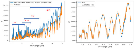
Figure 18.
(Left panel): Comparison between the simulated Jovian spectrum using the NEMESIS CIRS model and the observational data from ISO ([54]) as input. Several molecular bands are identified in the figure. The simulation is over-predicting the data. To correct this, the vertical abundance profile of the molecules highlighted in the figure were adjusted; (Right panel) best-fit simulation for the and absorption at 9–11 m.
The discrepancy between the observations and the model in Figure 18 does not explicitly imply that the CIRS model does not explain the ISO data. This discrepancy can be due to several factors such as different geometries, different abundance profiles and different altitudes sounded by the observations. The discrepancy at 9–11 m was solved after the retrieval was done for this wavelength interval (see Figure 18, right panel), obtaining two new and profiles that better fit the observations. The discrepancy between simulation and observations at 7–9 m is, however, significant. A retrieval was performed at this wavelength interval to adjust the vertical abundance profiles of and . However, this retrieval was not successful. This highly suggests that incorrect abundances of and are not the cause of the discrepancy. We also intend to study in future work the transmittance of other molecules such as , and to determine whether the absorption features of these molecules significantly contribute to the spectrum at 7–9 m. To evaluate the source of this discrepancy with certainty, further dedicated observations of Jupiter are needed at this wavelength interval.
5. Discussion and Conclusions
This work demonstrates that the Planetary Spectrum Generator (PSG) [55] is a highly effective tool to study the detection and perform the retrieval of chemical species in the solar system’s atmospheres in the context of several case studies such as minor chemical species, species of astrobiological interest and species related to atmospheric evolution.
In this framework, we performed a reanalysis of the observations regarding sulphur dioxide on Venus at 7.4 m [23], which allowed us to identify the molecules responsible for the absorption lines in the observations and agrees with the identification made by Encrenaz et al. [23]. In this work, the mean volume mixing ratio of obtained at the cloud top using the VIRA-2 model [60] was 120 ppb, which was consistent with that obtained by Encrenaz et al. [23]—50–175 ppb. Future reanalysis of the observations by TEXES of the 19 m and the 8.7 m bands will be performed by our group in future studies in order to constrain the vertical abundance profile at different altitude levels, complementing the results of this work.
From our reanalysis of the phosphine-related observations on Venus, at 10.5 m [22], we pinpointed the position of the phosphine absorption line in our simulations. However, we note that the strong telluric water absorption at 955.2–955.3 is an important obstacle to the detection of phosphine on Venus. The non-detection of phosphine, as in Encrenaz et al. [22], does not preclude the existence of phosphine on Venus. We must consider that only an upper limit of 7 ppb was derived and still has not confirmed [20,21,73]. One must also consider possible latitudinal, temporal and altitude variations in the abundance of phosphine. Considering these factors, the non-detection of phosphine may indicate that phosphine is not present at the probed altitude (cloud top) in sufficient abundance to be clearly detected [22]. Moreover, we must mention that IR wavelengths struggle to permeate below the cloud top; therefore, we do not have constraints on the abundance of phosphine below the cloud top. However, according to the work of Bains et al. [21], phosphine would be readily destroyed in this region. In sum, this means that further dedicated observations to search for phosphine on Venus should be performed. Presently, our group is analyzing ground-based observations of TEXES to search for phosphine on Venus in the NIR. To conclude, the detection of phosphine on Venus is extremely difficult due to the possible low abundance and overlapping of the phosphine absorption lines with those of sulphur dioxides which are present in much larger abundances, and telluric water absorption during ground-based observations, given the potential low abundances of phosphine.
Our reanalysis of the positive detection and non-detection of methane related to the MEx and ExoMars space probes [25,26] using PSG simulations allowed the identification of the molecules responsible for the absorption features identified in the studies by Giuranna et al. [25] and Korablev et al. [26]. Nevertheless, we were not successful in estimating the volume mixing ratio of methane due to issues regarding the definition of the instrument line shape of the PFS instrument in our simulations. Regarding our simulations of the observations by the ExoMars space probe, we want to emphasize that at approximately 3029 , where a methane absorption feature should be present according to Korablev et al. [26], there was no unique methane absorption feature present in our simulations. Instead, at the indicated wavenumber, we found an overlapping of several absorption lines and a strong methane absorption line. The discrepancy between the observations of the MEx and ExoMars space probes have not been explained to date. This discrepancy can be explained by the possible spatial and temporal variability of methane abundance [27,28,29,30,31,32]. Methane on Mars may have several sources and sinks. The sources of methane on Mars may be internal, such as volcanoes and hydrogeochemical processes involving serpentinization; exogenous, such as meteorites, comets and interplanetary dust; or even biological [74]. The conventional source of methane loss is photochemistry in the upper and middle atmosphere through UV photolysis and oxidation by O() and OH. However, in order to reconcile the detection and non-detection results from the Mars Express and ExoMars space probes, a fast destruction mechanism must be present. Several mechanisms for fast destruction have been proposed, such as energetic electrons resulting from the triboelectric process during convective dust storms [75], sequestration on airborne dust [76] and sequestration by superoxides from hydrogen peroxide in the surface/subsurface [77,78,79,80].
From our reanalysis of the observations of Mars taken by SOFIA by Encrenaz et al. [34], we obtained a D/H ratio value consistent with that obtained by Encrenaz et al. [34]. The obtained value was D/H ∼ 5.9 D/H (Earth), comparable with D/H = 3.4–4.8 D/H (Earth) [34].
Finally, from our reanalysis of ISO observations of Jupiter [54], we identified the source of the molecular absorption/emission bands in the data, agreeing with the identification made by Encrenaz et al. [54]. Furthermore, we obtained new vertical abundance profiles of and using the retrieval method that better fit the observations by ISO. The retrieved profile of is 2 times the initial profile and the retrieved profile of is 0.4 times the initial profile. Using the retrieval method, we could not correct for the discrepancy between the simulations and observations at 7–9 m. A retrieval was performed, as a side work, at this wavelength interval to adjust the vertical abundance profiles of and . However, this retrieval was not successful. This highly suggests that incorrect abundances of and in our model are not the cause of the discrepancy. We also intend to study the transmittance of other molecules such as , and to determine where the absorption features of these molecules significantly contribute to the spectrum at 7–9 m. To evaluate the source of this discrepancy with certainty, further dedicated observations of Jupiter are needed at this wavelength interval. The discrepancy at 7–9 m cannot be studied at present using a retrieval of the TP profile with PSG. Since, at this time, PSG does not allow this TP retrieval, we performed a dedicated simulation with the NEMESIS radiative transfer code [63] to retrieve the TP profile using the CIRS template model. The discrepancy decreased but was not solved completely. The retrieved T-P profile was used as input for a new PSG model, using the same abundance profiles as before. We then performed the retrieval of the scalers of the and abundance profiles in PSG. The resulting reduced did not improve. In future work, we will properly address this issue.
To sum up, PSG proved to be an efficient tool when studying and retrieving the abundances of minor chemical species in planetary atmospheres as well as compounds of astrobiological interest.
Author Contributions
Conceptualization, J.A.D. and P.M.; formal analysis, J.A.D. and P.M.; investigation, J.A.D., P.M. and J.R.; methodology, J.A.D. and P.M.; resources, J.A.D., P.M. and J.R.; supervision, P.M.; validation, J.A.D. and P.M.; visualization, J.A.D., P.M. and J.R.; writing—original draft, J.A.D. and P.M.; writing—review and editing, J.A.D., P.M. and J.R. All authors have read and agreed to the published version of the manuscript.
Funding
This research was funded by the Portuguese Fundação Para a Ciência e Tecnologia under project P-TUGA Ref. PTDC/FIS-AST/29942/2017 through national funds and by FEDER through COMPETE 2020 (Ref. POCI-01-0145 FEDER-007672).
Data Availability Statement
Data are available in a publicly accessible repository. The data presented in this study are openly available in “Machado, Pedro (2021)”, “Dataset JADias2021”, Mendeley Data, V1, http://dx.doi.org/10.17632/tpc5xzsy56.1, accessed on 7 March 2022.
Acknowledgments
We are grateful to Thérèse Encrenaz, from LESIA, Observatoire de Paris, for all the support and fruitful discussion; Gerónimo Villanueva, from NASA-Goddard Space Flight Center, for discussing issues regarding PSG; Marco Giuranna, PI of the PFS instrument of Mars Express (ESA), Alejandro Cardesín, from ESAC-ESA, Ann Carine Vandaele, PI of the NOMAD instrument of ExoMars (ESA), and Severine Robert, from the ExoMars team, for all the support regarding Mars dedicated research; Gabriella Gilli (IAA), for collaboration regarding the LMD-VGCM model; Patrick Irwin, from the University of Oxford (UK), for the collaboration under the NEMESIS radiative transfer code; Asier Munguira, from the University of the Basque Country, for their availability to discuss atmospheric research methods in the context of the present work.
Conflicts of Interest
The authors declare no conflict of interest.
References
- Zhang, X.; Liang, M.C.; Mills, F.P.; Belyaev, D.A.; Yung, Y.L. Sulfur chemistry in the middle atmosphere of Venus. Icarus 2012, 217, 714–739. [Google Scholar] [CrossRef]
- Marcq, E.; Mills, F.P.; Parkinson, C.D.; Vandaele, A.C. Composition and chemistry of the neutral atmosphere of Venus. Space Sci. Rev. 2017, 214, 1. [Google Scholar] [CrossRef] [Green Version]
- Jenkins, J.M.; Kolodner, M.A.; Butler, B.J.; Suleiman, S.H.; Steffes, P.G. Microwave remote sensing of the temperature and distribution of sulfur compounds in the lower atmosphere of Venus. Icarus 2002, 158, 312–328. [Google Scholar] [CrossRef]
- Butler, B. Accurate and consistent microwave observations of Venus and their implications. Icarus 2001, 154, 226–238. [Google Scholar] [CrossRef]
- Oyama, V.I.; Carle, G.C.; Woeller, F.; Pollack, J.B.; Reynolds, R.T.; Craig, R.A. Craig; Pioneer Venus gas chromatography of the lower atmosphere of Venus. J. Geophys. Res. 1980, 85, 7891–7902. [Google Scholar] [CrossRef]
- Marcq, E.; Encrenaz, T.; Bézard, B.; Birlan, M. Remote Sensing of Venus’ lower atmosphere from ground-based IR spectroscopy: Latitudinal and vertical distribution of minor species. Planet. Space Sci. 2005, 54, 1360–1370. [Google Scholar] [CrossRef]
- Jenkins, J.M.; Steffes, P.G.; Hinson, D.P.; Twicken, J.D.; Tyler, G. Leonard; Radio occultation studies of the Venus atmosphere with the Magellan spacecraft. Icarus 1994, 110, 79–94. [Google Scholar] [CrossRef]
- Gubenko, V.N.; Yakovlev, O.I.; Matyugov, S.S. Radio Occultation Measurements of the Radio Wave Absorption and the Sulfuric Acid Vapor Content in the Atmosphere of Venus. Cosm. Res. 2001, 39, 439–445. [Google Scholar] [CrossRef]
- Mallama, A.; Wang, D.; Howard, R.A. Venus phase function and forward scattering from H2SO4. Icarus 2006, 182, 10–22. [Google Scholar] [CrossRef]
- Bézard, B.; Bergh, C.D. Composition of the atmosphere of Venus below the clouds. J. Geophys. Res. 2007, 112, E04S07. [Google Scholar] [CrossRef]
- Zasova, L.; Moroz, V.; Esposito, L.; Na, C. SO2 in the middle atmosphere of Venus: IR measurements from VENERA-15 and comparison to UV data. Icarus 1993, 105, 92–109. [Google Scholar] [CrossRef]
- Marcq, E.; Belyaev, D.; Montmessin, F.; Fedorova, A.; Bertaux, J.-L.; Vandaele, A.C.; Neefs, E. An investigation of the SO2 content of the venusian mesosphere using SPICAV-UV in nadir mode. Icarus 2011, 211, 58–69. [Google Scholar] [CrossRef]
- Encrenaz, T.; Greathouse, T.; Marcq, E.; Sagawa, H.; Widemann, T.; Bézard, B.; Fouchet, T.; Lefèvre, F.; Lebonnois, S.; Atreya, S.; et al. HDO and SO2 thermal mapping on Venus. V. Evidence for a long-term anti-correlation. Astron. Astrophys. 2020, 543, A69. [Google Scholar] [CrossRef]
- Schwieterman, E.; Kiang, N.; Parenteau, M.; Harman, C.; DasSarma, S.; Fisher, T.; Arney, G.; Hartnett, H.; Reinhard, C.; Olson, S.; et al. Exoplanet Biosignatures: A Review of Remotely Detectable Signs of Life. Astrobiology 2018, 18, 663–708. [Google Scholar] [CrossRef] [PubMed]
- Sousa-Silva, C. Phosphine as a Biosignature Gas in Exoplanet Atmospheres. Astrobiology 2020, 20, 235–268. [Google Scholar] [CrossRef] [PubMed]
- Morton, S.C.; Edwards, M. Reduced phosphorus compounds in the environment. Crit. Rev. Environ. Sci. Technol. 2005, 35, 333–364. [Google Scholar] [CrossRef]
- Pasek, M.A.; Sampson, J.M.; Atlas, Z. Redox chemistry in the phosphorus biogeochemical cycle. Proc. Natl. Acad. Sci. USA 2014, 111, 15468–15473. [Google Scholar] [CrossRef] [PubMed] [Green Version]
- Irwin, P. Giant Planets of Our Solar System: Atmospheres, Composition, and Structure; Springer: Berlin, Germany, 2010. [Google Scholar]
- Greaves, J.S.; Richards, A.M.S.; Bains, W.; Rimmer, P.B.; Sagawa, H.; Clements, D.L.; Seager, S.; Petkowski, J.J.; Sousa-Silva, C.; Ranjan, S.; et al. Phosphine gas in the cloud decks of Venus. Nat. Astron. 2020, 5, 655–664. [Google Scholar] [CrossRef]
- Greaves, J.S.; Richards, A.M.S.; Bains, W.; Rimmer, P.B.; Clements, D.L.; Seager, S.; Petkowski, J.J.; Sousa-Silva, C.; Ranjan, S.; Fraser, H.J. Reply to: No evidence of phosphine in the atmosphere of Venus from independent analyses. Nat. Astron. 2021, 5, 636–639. [Google Scholar] [CrossRef]
- Bains, W.; Petkowski, J.J.; Seager, S.; Ranjan, S.; Sousa-Silva, C.; Rimmer, P.B.; Zhan, Z.; Greaves, J.S.; Richards, A.M. Phosphine on Venus cannot be explained by conventional processes. Astrobiology 2021, 21, 1277–1304. [Google Scholar] [CrossRef]
- Encrenaz, T.; Greathouse, T.; Marcq, E.; Widemann, T.; Bézard, B.; Fouchet, T.; Giles, R.; Sagawa, H.; Greaves, J.; Sousa-Silva, C. A stringent upper limit of the PH3 abundance at the cloud top of Venus. Astron. Astrophys. 2020, 643, L5. [Google Scholar] [CrossRef]
- Encrenaz, T.; Greathouse, T.K.; Roe, H.G.; Richter, M.J.; Lacy, J.H.; Bézard, B.; Fouchet, T.; Widemann, T. HDO and SO2 thermal mapping on Venus: Evidence for strong SO2 variability. Astron. Astrophys. 2012, 543, A153. [Google Scholar] [CrossRef] [Green Version]
- Krasnopolsky, V.A.; Maillard, J.P.; Owen, T.C. Detection of methane in the martian atmosphere: Evidence for life? Icarus 2004, 172, 537–547. [Google Scholar] [CrossRef]
- Giuranna, M.; Viscardy, S.; Daerden, F.; Neary, L.; Etiope, G.; Oehler, D.; Formisano, V.; Aron-ica, A.; Wolkenberg, P.; Aoki, S.; et al. Independent confirmation of a methane spike on Mars and a source region east of gale crater. Nat. Geosci. 2019, 12, 326–332. [Google Scholar] [CrossRef]
- Korablev, O.; Vandaele, A.C.; Montmessin, F.; Fedorova, A.A.; Trokhimovskiy, A.; Forget, F.; Lefèvre, F.; Daerden, F.; Thomas, I.R.; Trompet, L.; et al. No detection of methane on Mars from early ExoMars Trace Gas Orbiter observations. Nature 2019, 568, 517–520. [Google Scholar] [CrossRef] [PubMed]
- Etiope, G.; Oehler, D.Z. Methane spikes, background seasonality and non-detections on Mars: A geological perspective. Planet. Space Sci. 2019, 168, 52–61. [Google Scholar] [CrossRef]
- Moores, J.E.; Gough, R.V.; Martinez, G.M.; Meslin, P.-Y.; Smith, C.L.; Atreya, S.K.; Mahaffy, P.R.; Newman, C.E.; Webster, C.R. Methane seasonal cycle at Gale Crater on Mars consistent with regolith adsorption and diffusion. Nat. Geosci. 2019, 12, 321–325. [Google Scholar] [CrossRef]
- Moores, J.E.; King, P.L.; Smith, C.L.; Martinez, G.M.; Newman, C.E.; Guzewich, S.D.; Meslin, P.; Webster, C.R.; Mahaffy, P.R.; Atreya, S.K.; et al. The methane diurnal variation and microseepage flux at Gale Crater, Mars as constrained by the ExoMars trace gas orbiter and Curiosity Observations. Geophys. Res. Lett. 2019, 46, 9430–9438. [Google Scholar] [CrossRef]
- Knutsen, E.W.; Villanueva, G.L.; Liuzzi, G.; Crismani, M.M.; Mumma, M.J.; Smith, M.D.; Vandaele, A.C.; Aoki, S.; Thomas, I.R.; Daerden, F.; et al. Comprehensive investigation of Mars methane and organics with ExoMars/NOMAD. Icarus 2021, 357, 114266. [Google Scholar] [CrossRef]
- Webster, C.R.; Mahaffy, P.R.; Pla-Garcia, J.; Rafkin, S.C.R.; Moores, J.E.; Atreya, S.K.; Flesch, G.J.; Malespin, C.A.; Teinturier, S.M.; Kalucha, H.; et al. Day-night differences in Mars methane suggest nighttime containment at Gale crater. Astron. Astrophys. 2021, 650, A166. [Google Scholar] [CrossRef]
- Montmessin, F.; Korablev, O.I.; Trokhimovskiy, A.; Lefèvre, F.; Fedorova, A.A.; Baggio, L.; Irbah, A.; Lacombe, G.; Olsen, K.S.; Braude, A.S.; et al. A stringent upper limit of 20 pptv for methane on Mars and constraints on its dispersion outside Gale crater. Astron. Astrophys. 2021, 650, A140. [Google Scholar] [CrossRef]
- Encrenaz, T.; Roques, F.; Bibring, J.-P.; Zarka, P.; Blanc, M.; Barucci, M.-A. The Solar System; Dunlop, S., Translator; Springer: Berlin/Heidelberg, Germany; New York, NY, USA, 2010. [Google Scholar]
- Encrenaz, T.; Dewitt, C.; Richter, M.J.; Greathouse, T.K.; Fouchet, T.; Montmessin, F.; Lefèvre, F.; Bézard, B.; Atreya, S.K.; Aoki, S.; et al. New measurements of D/H on Mars using Exes aboard SOFIA. Astron. Astrophys. 2018, 612, A112. [Google Scholar] [CrossRef] [Green Version]
- Villanueva, G.L.; Liuzzi, G.; Crismani, M.M.J.; Aoki, S.; Vandaele, A.C.; Daerden, F.; Smith, M.D.; Mumma, M.J.; Knutsen, E.W.; Neary, L.; et al. Water heavily fractionated as it ascends on marsas revealed by ExoMars/NOMAD. Sci. Adv. 2021, 7, eabc8843. [Google Scholar] [CrossRef]
- Sánchez-Lavega, A. An Introduction to Planetary Atmospheres; CRC Press: Boca Raton, FL, USA, 2011. [Google Scholar]
- Vago, J.L.; Westall, F.; Pasteur Instrument Teams; Landing Site Selection Working Group; Coates, A.J.; Jaumann, R.; Korablev, O.; Ciarletti, V.; Mitrofanov, I.; Josset, J.-L.; et al. Habitability on early Mars and the search for biosignatures with the ExoMars Rover. Astrobiology 2017, 17, 471–510. [Google Scholar] [CrossRef] [PubMed]
- Greenwood, J.P.; Itoh, S.; Sakamoto, N.; Vicenzi, E.; Yurimoto, H. Hydrogen isotope evidence for loss of water from Mars through Time. Geophys. Res. Lett. 2008, 35, 5. [Google Scholar] [CrossRef] [Green Version]
- Usui, T.; Alexander, C.; Wang, J.; Simon, J.I.; Jones, J.H. Origin of water and mantle–crust interactions on Mars inferred from hydrogen isotopes and volatile element abundances of olivine-hosted melt inclusions of primitive shergottites. Earth Planet. Sci. Lett. 2012, 357–358, 119–129. [Google Scholar] [CrossRef]
- Mahaffy, P.R.; Webster, C.R.; Stern, J.C.; Brunner, A.E.; Atreya, S.K.; Conrad, P.G.; Domagal-Goldman, S.; Eigenbrode, J.L.; Flesch, G.J.; Christensen, L.E.; et al. The imprint of atmospheric evolution in the D/H of Hesperian Clay Minerals on Mars. Science 2015, 347, 412–414. [Google Scholar] [CrossRef] [Green Version]
- Novak, R.E.; Mumma, M.J.; Villanueva, G.L. Measurement of the isotopic signatures of water on Mars; implications for studying methane. Planet. Space Sci. 2011, 59, 163–168. [Google Scholar] [CrossRef]
- Villanueva, G.L.; Mumma, M.J.; Novak, R.E.; Käufl, H.U.; Hartogh, P.; Encrenaz, T.; Tokunaga, A.; Khayat, A.; Smith, M.D. Strong water isotopic anomalies in the martian atmosphere: Probing current and Ancient Reservoirs. Science 2015, 348, 218–221. [Google Scholar] [CrossRef] [Green Version]
- Krasnopolsky, V.A. Variations of the HDO/H2O ratio in the martian atmosphere and loss of water from Mars. Icarus 2015, 257, 377–386. [Google Scholar] [CrossRef]
- Aoki, S.; Nakagawa, H.; Sagawa, H.; Giuranna, M.; Sindoni, G.; Aronica, A.; Kasaba, Y. Seasonal variation of the HDO/H2O ratio in the atmosphere of Mars at the middle of northern spring and beginning of Northern Summer. Icarus 2015, 260, 7–22. [Google Scholar] [CrossRef]
- Encrenaz, T.; DeWitt, C.; Richter, M.J.; Greathouse, T.K.; Fouchet, T.; Montmessin, F.; Lefèvre, F.; Forget, F.; Bézard, B.; Atreya, S.K.; et al. A map of D/H on Mars in the thermal infrared using EXES aboard SOFIA. Astron. Astrophys. 2016, 586, A62. [Google Scholar] [CrossRef]
- Owen, T.; Maillard, J.P.; de Bergh, C.; Lutz, B.L. Deuterium on Mars: The Abundance of HDO and the Value of D/H. Science 1988, 240, 1767. [Google Scholar] [CrossRef] [PubMed]
- Donahue, T.M.; Hodges, R.R. Past and present water budget of Venus. J. Geophys. Res. 1992, 97, 6083–6091. [Google Scholar] [CrossRef]
- Fedorova, A.; Korablev, O.; Vandaele, A.-C.; Bertaux, J.-L.; Belyaev, D.; Mahieux, A.; Neefs, E.; Wilquet, W.V.; Drummond, R.; Montmessin, F.; et al. HDO and H2O vertical distributions and isotopic ratio in the Venus mesosphere by Solar Occultation at Infrared spectrometer on board Venus Express. J. Geophys. Res. 2008, 113, E5. [Google Scholar] [CrossRef] [Green Version]
- Gettelman, A.; Webster, C.R. Simulations of water isotope abundances in the upper troposphere and lower stratosphere and implications for stratosphere troposphere exchange. J. Geophys. Res. 2005, 110, 17301. [Google Scholar] [CrossRef] [Green Version]
- Villanueva, G.L.; Mumma, M.J.; Bonev, B.P.; Novak, R.E.; Barber, R.J.; DiSanti, M.A. Water in planetary and cometary atmospheres: H2O/HDO transmittance and fluorescence models. J. Quant. Spectrosc. Radiat. Transf. 2012, 113, 202–220. [Google Scholar] [CrossRef] [Green Version]
- Webster, C.R.; Mahaffy, P.R.; Atreya, S.K.; Flesch, G.J.; Mischna, M.A.; Meslin, P.-Y.; Farley, K.A.; Conrad, P.G.; Christensen, L.E.; Pavlov, A.A.; et al. Mars methane detection and variability at Gale Crater. Science 2015, 347, 415–417. [Google Scholar] [CrossRef] [Green Version]
- Albert, S.; Bauerecker, S.; Boudon, V.; Brown, L.R.; Champion, J.P.; Loëte, M.; Nikitin, A.; Quack, M. Global Analysis of the high resolution infrared spectrum of methane 12CH4 in the region from 0 to 4800 cm−1. Chem. Phys. 2008, 356, 131–146. [Google Scholar] [CrossRef]
- Mumma, M.J.; Villanueva, G.L.; Novak, R.E.; Hewagama, T.; Bonev, B.P.; DiSanti, M.A.; Mandell, A.M.; Smith, M.D. Strong Release of Methane on Mars in Northern Summer 2003. Science 2009, 323, 1041–1045. [Google Scholar] [CrossRef] [Green Version]
- Encrenaz, T.; Drossart, P.; Feuchtgruber, H.; Lellouch, E.; Bézard, B.; Fouchet, T.; Atreya, S. The atmospheric composition and structure of Jupiter and Saturn from ISO observations: A preliminary review. Planet. Space Sci. 1999, 47, 1225–1242. [Google Scholar] [CrossRef] [Green Version]
- Villanueva, G.; Smith, M.; Protopapa, S.; Faggi, S.; Mandell, A. Planetary spectrum generator: An accurate online radiative transfer suite for atmospheres, comets, small bodies and exoplanets. J. Quant. Spectrosc. Radiat. Transf. 2018, 217, 86–104. [Google Scholar] [CrossRef] [Green Version]
- Gordon, I.E.; Rothman, L.S.; Hargreaves, R.J.; Hashemi, R.; Karlovets, E.V.; Skinner, F.M.; Conway, E.K.; Hill, C.; Kochanov, R.V.; Tan, Y.; et al. The HITRAN 2020 molecular spectroscopic database. J. Quant. Spectrosc. Radiat. Transf. 2021, 277, 107949. [Google Scholar] [CrossRef]
- Rodger, C.D. Inverse Methods for Atmospheric Sounding: Theory and Practice; World Scientific: Singapore, 2008. [Google Scholar]
- Gilli, G.; Lebonnois, S.; González-Galindo, F.; López-Valverde, M.A.; Stolzenbach, A.; Lefèvre, F.; Chaufray, J.Y.; Lott, F. Thermal structure of the upper atmosphere of Venus simulated by a ground-to-thermosphere GCM. Icarus 2017, 281, 55–72. [Google Scholar] [CrossRef]
- Garate-Lopez, I.; Lebonnois, S. Latitudinal variation of clouds’ structure responsible for Venus’ cold collar. Icarus 2018, 314, 1–11. [Google Scholar] [CrossRef] [Green Version]
- Zasova, L.V.; Moroz, V.I.; Linkin, V.M.; Khatuntsev, I.V.; Maiorov, B.S. Structure of the Venusian atmosphere from surface up to 100 km. Cosm. Res. 2006, 44, 364–383. [Google Scholar] [CrossRef]
- Forget, F.; Hourdin, F.; Fournier, R.; Hourdin, C.; Talagrand, O.; Collins, M.; Lewis, S.R.; Read, P.L.; Huot, J.-P. Improved general circulation models of the Martian atmosphere from the surface to above 80 km. J. Geophys. Res. 1999, 104, 24155–24175. [Google Scholar] [CrossRef]
- Millour, E.; Forget, F.; Vals, A.S.M.; Zakharov, V.; Montabone, L.; Montmessin, F.L.F.; Chaufray, J.-Y.; López-Valverde, M.A.; González-Galindo, F.; Lewis, S.R.; et al. The Mars Climate Database (Version 5.3). In Proceedings of the Scientific Workshop: “From Mars Express to ExoMars”, Madrid, Spain, 27–28 February 2018. [Google Scholar]
- Irwin, P.G.J.; Teanby, N.A.; de Kok, R.; Fletcher, L.N.; Howett, C.J.A.; Tsang, C.C.C.; Wilson, C.F.; Calcutt, S.B.; Nixon, C.A.; Parrish, P.D. The NEMESIS planetary atmosphere radiative transfer and retrieval tool. J. Quant. Spectrosc. Rad. Trans. 2008, 109, 1136–1150. [Google Scholar] [CrossRef]
- Henningsen, J.; Barbe, A.; De Backer-Barilly, M.-R. Revised molecular parameters for 32SO2 and 34SO2 from high resolution study of the infrared spectrum in the 7–8 μm wavelength region. J. Quant. Spectrosc. Radiat. Transf. 2008, 109, 2491–2510. [Google Scholar] [CrossRef]
- Underwood, D.S.; Tennyson, J.; Yurchenko, S.N.; Huang, X.; Schwenke, D.W.; Lee, T.J.; Clausen, S.; Fateev, A. ExoMol molecular line lists—XIV. The rotation-vibration spectrum of hot SO2. Mon. Not. R. Astron. Soc. 2016, 459, 3890–3899. [Google Scholar] [CrossRef] [Green Version]
- Zak, E.; Tennyson, J.; Polyansky, O.L.; Lodi, L.; Zobov, N.F.; Tashkun, S.A.; Perevalov, V.I. A room temperature CO2 line list with ab initio computed intensities. J. Quant. Spectrosc. Radiat. Transf. 2016, 177, 31–42. [Google Scholar] [CrossRef] [Green Version]
- Tashkun, S.A.; Perevalov, V.I.; Gamache, R.R.; Lamouroux, J. CDSD-296 high resolution carbon dioxide spectroscopic databank: An update. J. Quant. Spectrosc. Radiat. Transf. 2019, 228, 124–131. [Google Scholar] [CrossRef]
- Kyuberis, A.A.; Zobov, N.F.; Naumenko, O.V.; Voronin, B.A.; Polyansky, O.L.; Lodi, L.; Liu, A.; Hu, S.-M.; Tennyson, J. Room temperature line lists for deuterated water. J. Quant. Spectrosc. Radiat. Transf. 2017, 203, 175–185. [Google Scholar] [CrossRef]
- Encrenaz, T.; Greathouse, T.K.; Richter, M.J.; Bézard, B.; Fouchet, T.; Lefèvre, F.; Montmessin, F.; Forget, F.; Lebonnois, S.; Atreya, S.K.; et al. Simultaneous mapping of H2O and H2O2 on Mars from infrared high-resolution imaging spectroscopy. Icarus 2008, 195, 547–556. [Google Scholar] [CrossRef]
- Brown, L.R.; Sams, R.L.; Kleiner, I.; Cottaz, C.; Sagui, L. Line intensities of the phosphine dyad at 10 μm. J. Mol. Spectrosc. 2002, 215, 178–203. [Google Scholar] [CrossRef]
- Lefèvre, F.; Forget, F. Observed variations of methane on Mars unexplained by known atmospheric chemistry and physics. Nature 2009, 460, 720–723. [Google Scholar] [CrossRef]
- Mischna, M.A.; Allen, M.; Richardson, M.I.; Newman, C.E.; Toigo, A.D. Atmospheric modeling of Mars methane surface releases. Planet. Space Sci. 2011, 59, 227–237. [Google Scholar] [CrossRef]
- Villanueva, G.L.; Cordiner, M.; Irwin, P.G.J.; de Pater, I.; Butler, B.; Gurwell, M.; Milam, S.N.; Nixon, C.A.; Luszcz-Cook, S.H.; Wilson, C.F.; et al. No evidence of phosphine in the atmosphere of Venus from independent analyses. Nat. Astron. 2020, 5, 631–635. [Google Scholar] [CrossRef]
- Atreya, S.K.; Mahaffy, P.R.; Wong, A.-S. Methane and related trace species on Mars: Origin, loss, implications for life, and Habitability. Planet. Space Sci. 2007, 55, 358–369. [Google Scholar] [CrossRef]
- Farrell, W.M.; Delory, G.T.; Atreya, S.K. Martian dust storms as a possible sink of atmospheric methane. Geophys. Res. Lett. 2006, 33, 21. [Google Scholar] [CrossRef] [Green Version]
- Jensen, S.J.K.; Skibsted, J.; Jakobsen, H.J.; Kate, I.L.T.; Gunnlaugsson, H.P.; Merrison, J.P.; Finster, K.; Bak, E.; Iversen, J.J.; Kondrup, J.C.; et al. A sink for methane on Mars? The answer is blowing in the wind. Icarus 2014, 236, 24–27. [Google Scholar] [CrossRef]
- DeLory, G.T.; Farrell, W.M.; Atreya, S.K.; Renno, N.O.; Wong, A.-S.; Cummer, S.A.; Sentman, D.D.; Marshall, J.R.; Rafkin, S.C.; Catling, D.C. Oxidant Enhancement in Martian Dust Devils and Storms: Storm Electric Fields and Electron Dissociative Attachment. Astrobiology 2006, 6, 51–52. [Google Scholar] [CrossRef] [PubMed]
- Atreya, S.K.; Wong, A.-S.; Renno, N.O.; Farrell, W.M.; DeLory, G.T.; Sentman, D.D.; Cummer, S.A.; Marshall, J.R.; Rafkin, S.C.R.; Catling, D. Oxidant Enhancement in Martian Dust Devils and Storms: Implications for Life and Habitability. Astrobiology 2006, 6, 439–450. [Google Scholar] [CrossRef] [Green Version]
- Atreya, S.K.; Witasse, O.; Chevrier, V.F.; Forget, F.; Mahaffy, P.R.; Price, P.B.; Webster, C.R.; Zurek, R.W. Methane on Mars: Current observations, interpretation, and future plans. Planet. Space Sci. 2011, 59, 133–136. [Google Scholar] [CrossRef]
- Atreya, S.K.; Encrenaz, T.; Korablev, O.; Mahaffy, P.R.; Moores, J.E.; Vandaele, A.C.; Webster, C.R.; Meslin, P.; Navarro-Gonzalez, R. Methane on Mars from MSL-Curiosity and ExoMars-Trace Gas Orbiter: A Destructive Role of Surface Oxidants? In Proceedings of the Ninth International Conference on Mars, Pasadena, CA, USA, 22–25 July 2019. LPI Contribution No. 2089, id.6067. [Google Scholar]
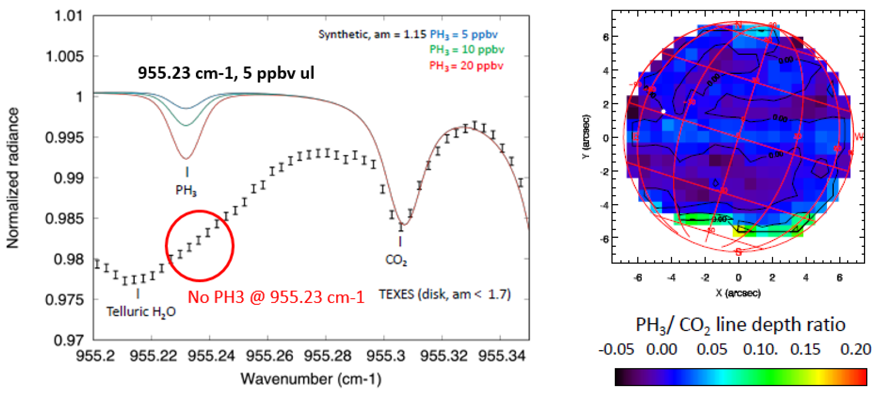
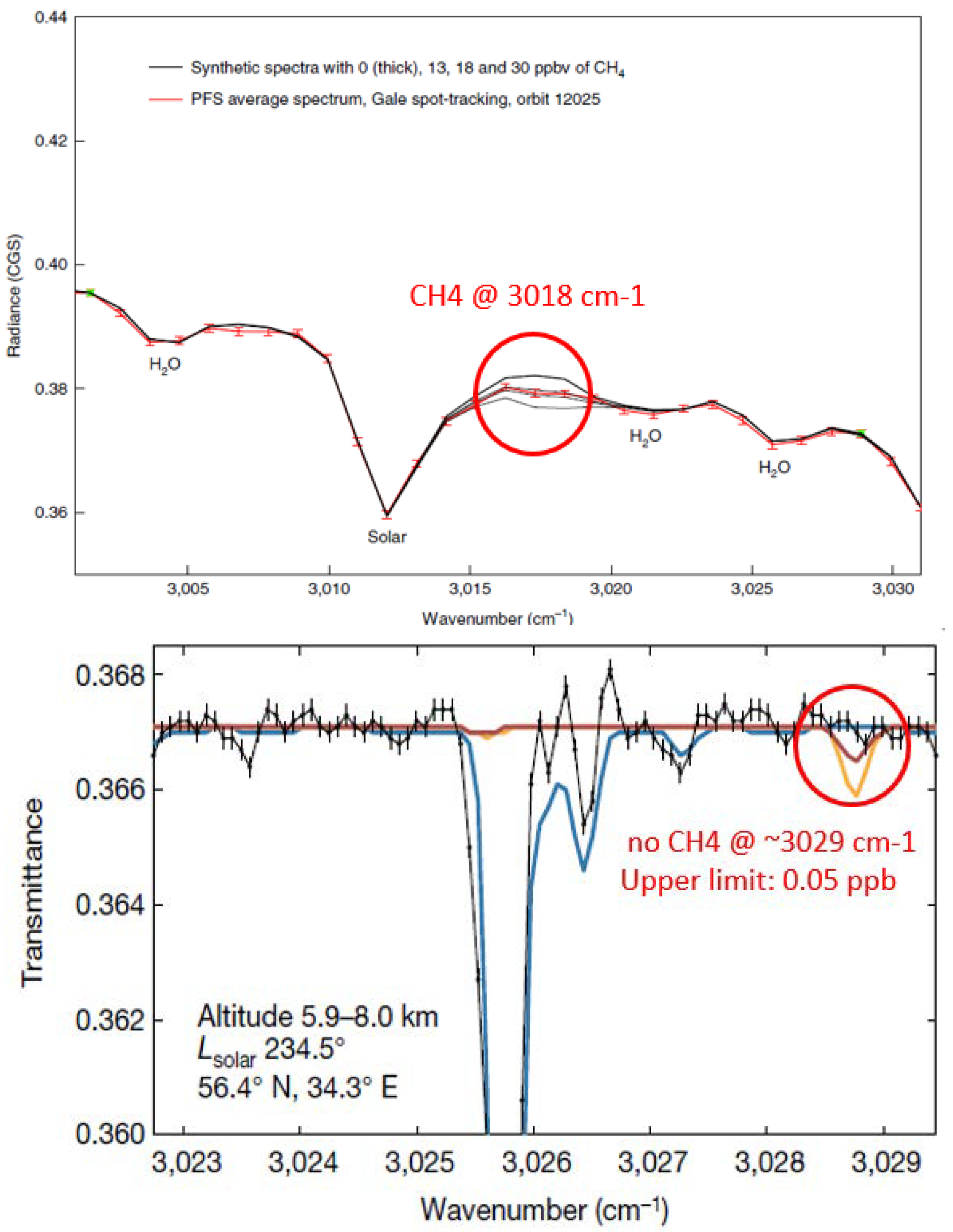
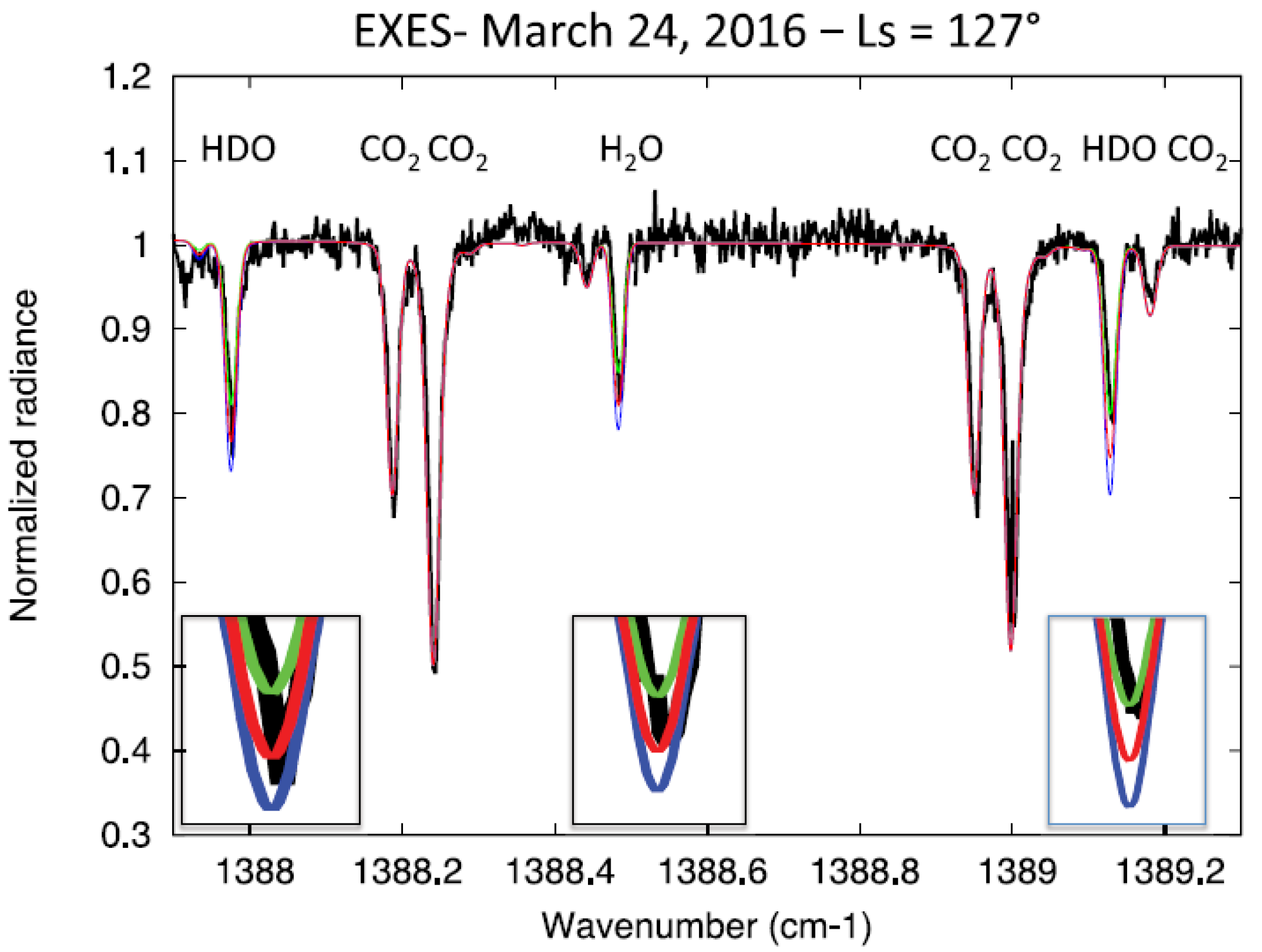
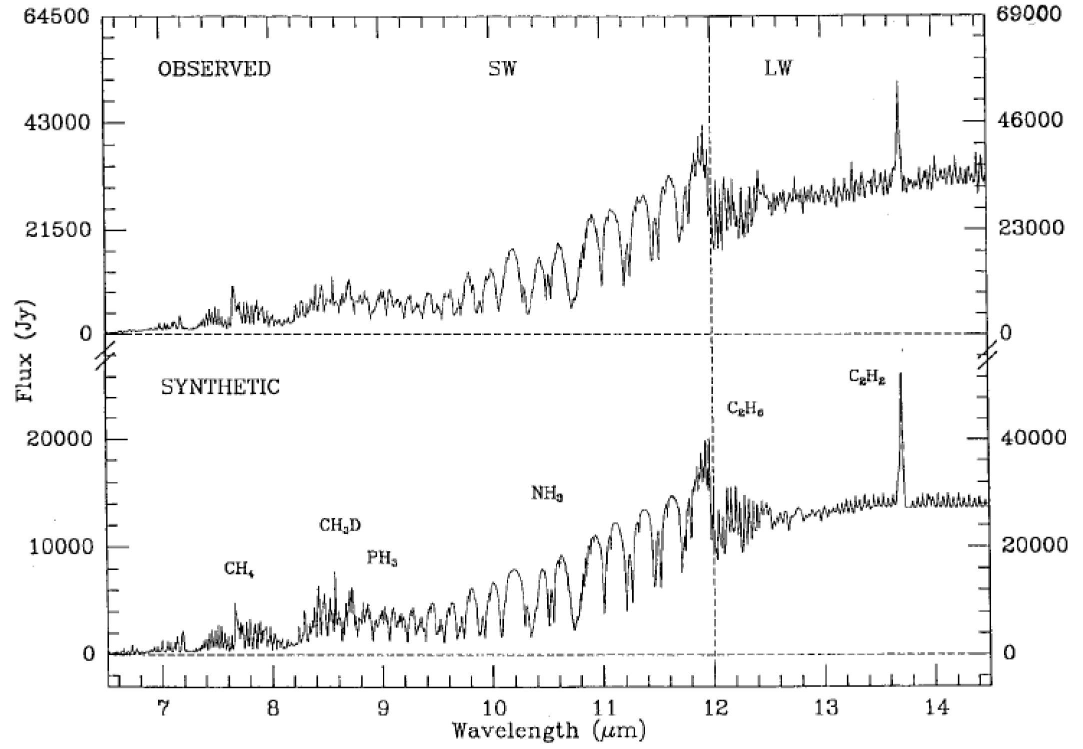
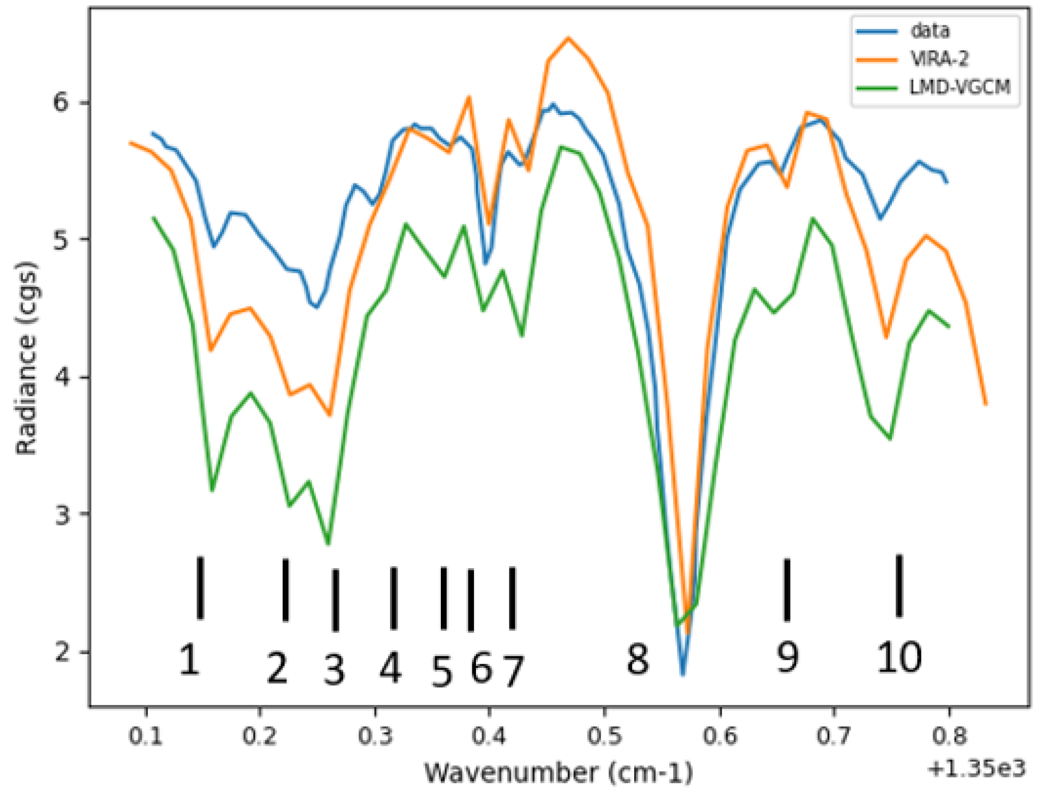


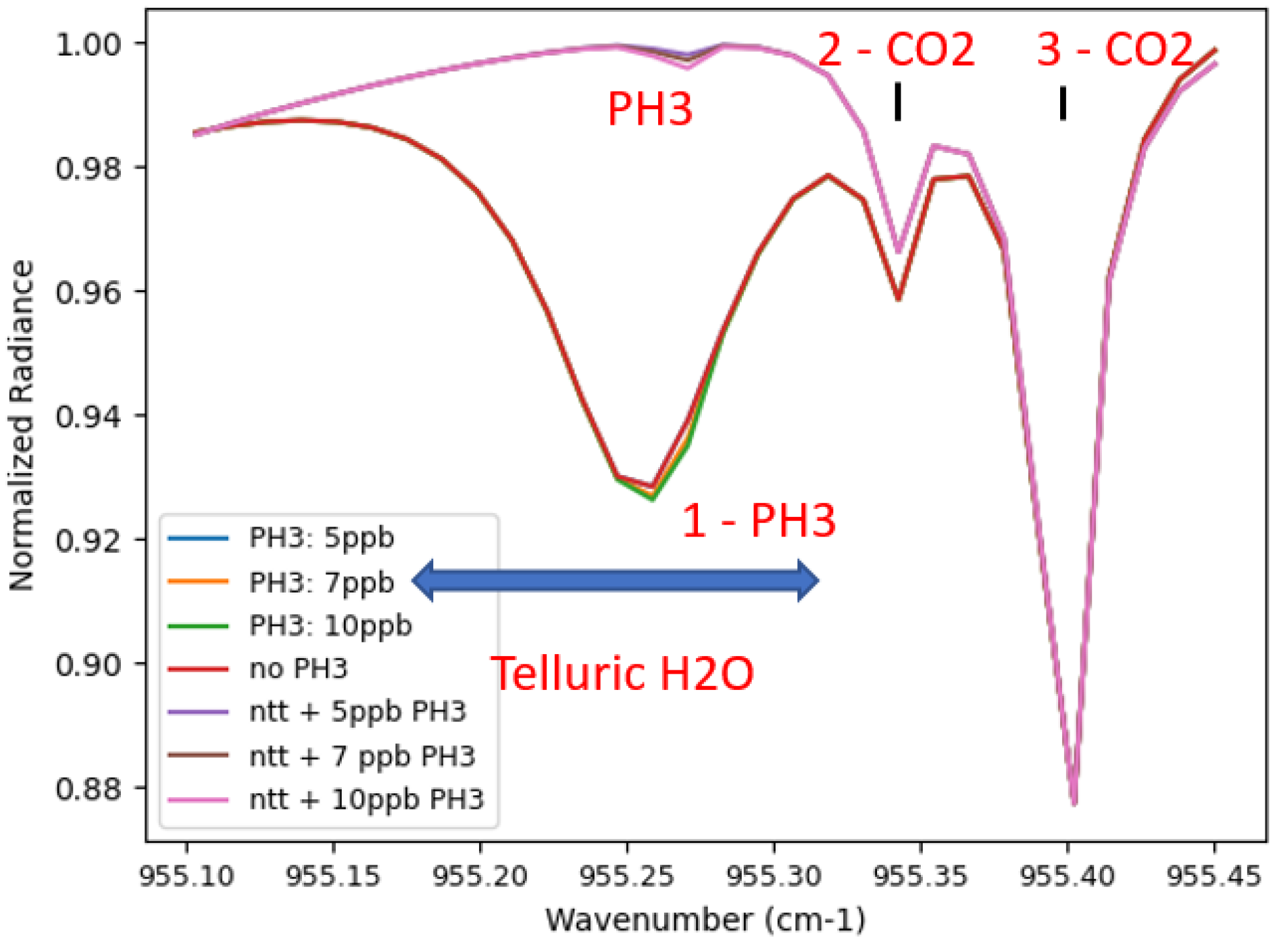
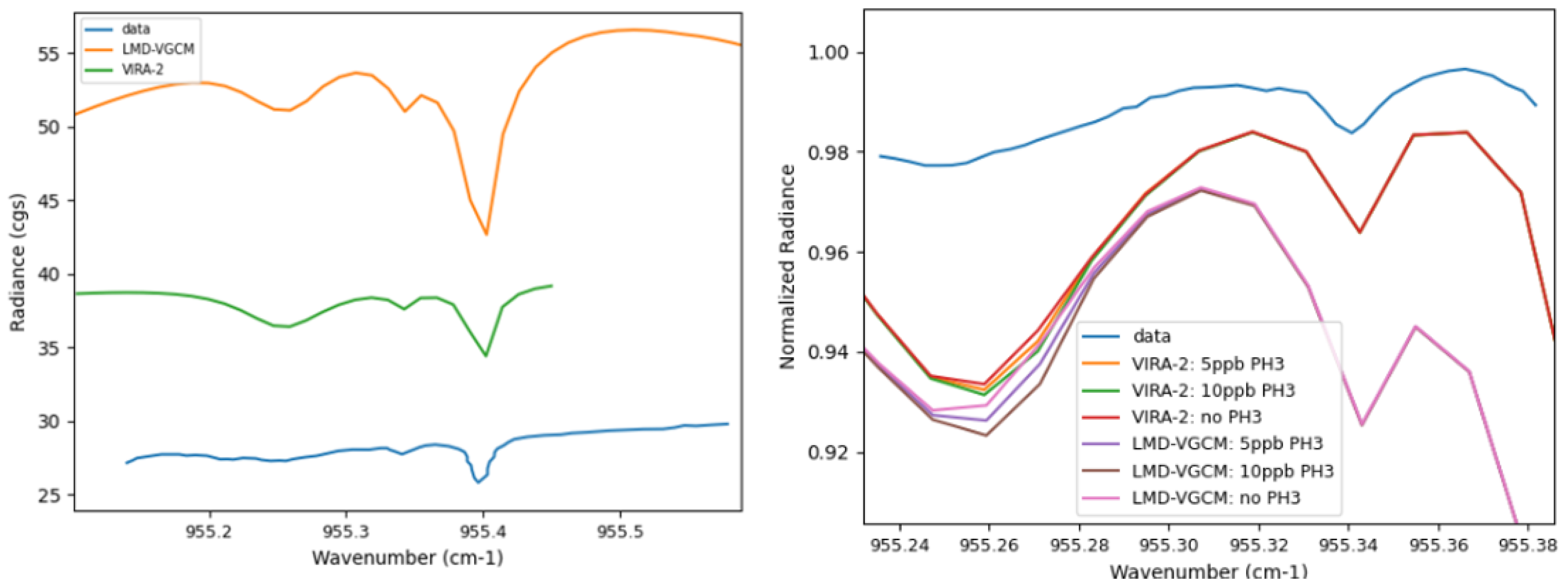

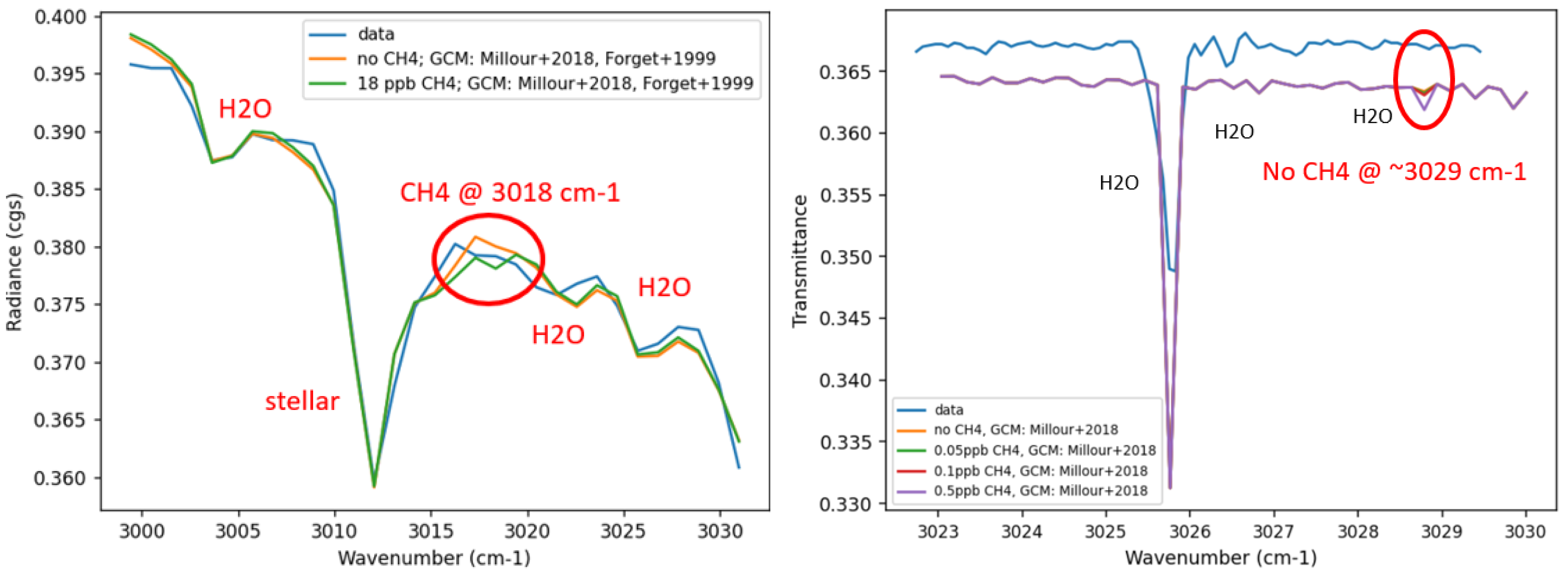
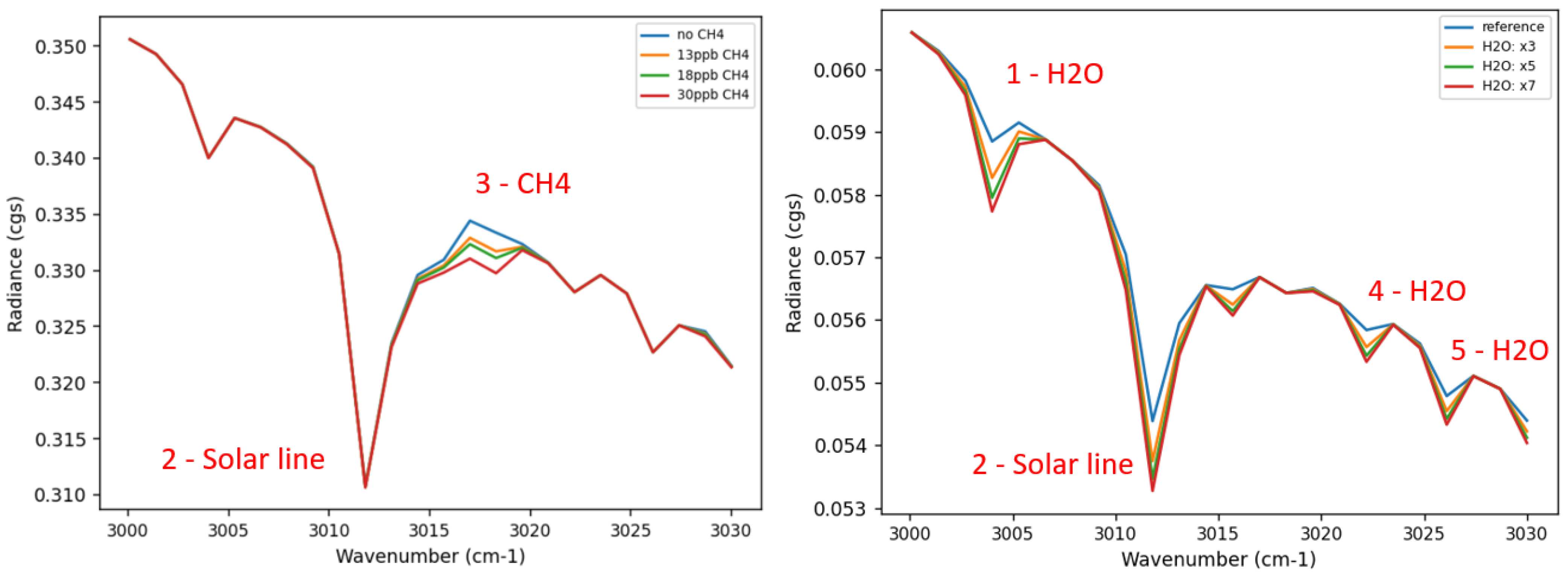
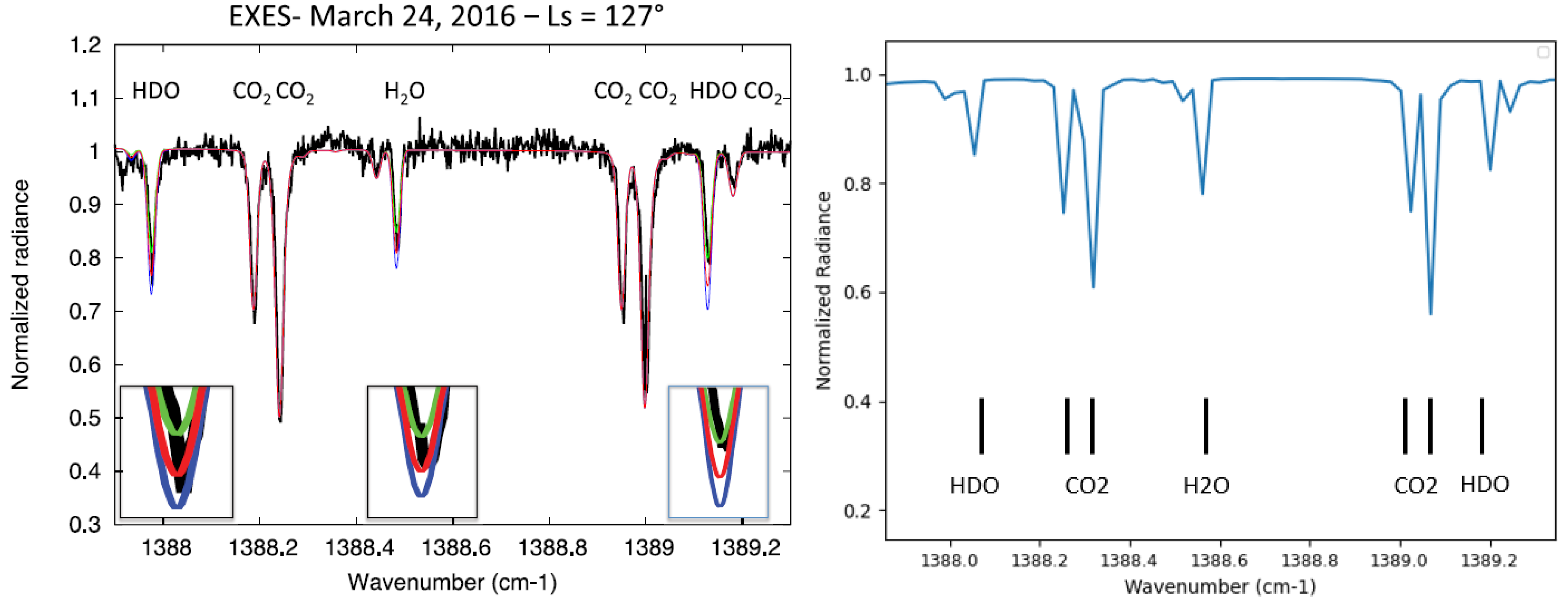

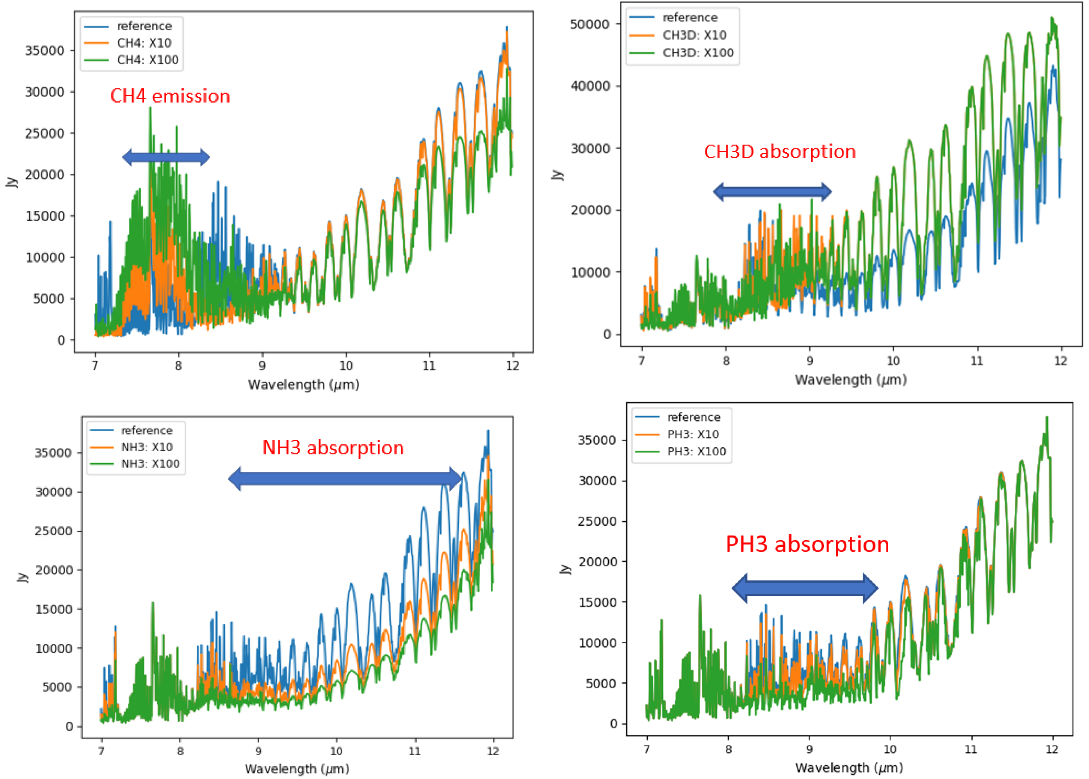
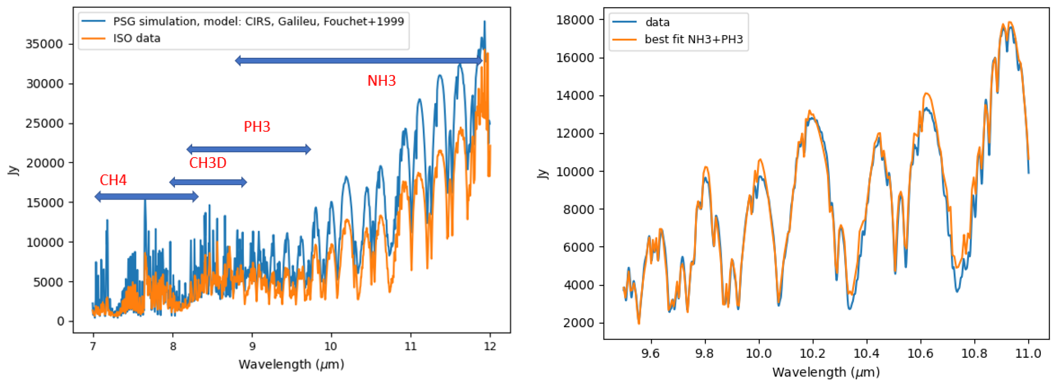
Publisher’s Note: MDPI stays neutral with regard to jurisdictional claims in published maps and institutional affiliations. |
© 2022 by the authors. Licensee MDPI, Basel, Switzerland. This article is an open access article distributed under the terms and conditions of the Creative Commons Attribution (CC BY) license (https://creativecommons.org/licenses/by/4.0/).