Extended North Atlantic Oscillation and Greenland Blocking Indices 1800–2020 from New Meteorological Reanalysis

Abstract

Based on newly-available meteorological reanalysis, we compile and present extended seasonal series of the North Atlantic Oscillation (NAO) and Greenland Blocking indices spanning 1800–2020, which we analyse for evidence of significant trends. This represents a major backward extension of the previously available instrumental-/reanalysis-based Azores–Iceland and principal component-based NAO indices, and allows us to evaluate the potential effect of natural climate perturbations, especially the 1809 and 1815 major volcanic eruptions and ~1790s–1830 Dalton solar minimum, on North Atlantic atmospheric circulation. We find that winters 1809/10 and 1816/17 mark positive NAO peaks, relative to several years before and afterwards, which is in accordance with the theory of volcanic forcing of climate. However, there is little evidence of a summer NAO volcanic signature. Overall, based on the significantly longer new reanalysis time series, the new series presented here corroborate and extend our previous results of: (1) a significantly more variable year-to-year NAO with a recent exceptional clustering of extreme events since 2000 for winter; (2) a significant increasing trend in blocking over Greenland in summer. These trends have major repercussions for the probability of the occurrence of extreme weather events over northwest Europe and for the sensitivity and response of the Greenland Ice Sheet to global warming, especially if they continue as an integral part of anthropogenic climate change.

1. Introduction

The North Atlantic Oscillation (NAO) is a widely-used measure of North Atlantic polar jet stream variation (mainly the north–south position of the jet), which is an important control of climatic conditions and extreme weather fluctuations across the UK, Northwest Europe and eastern North America [1,2,3,4]. The NAO is variously measured using a south minus north mean sea-level pressure difference (typically Azores–Iceland but sometimes using Lisbon or Gibraltar as the southern station) or a principal component analysis of gridded pressure or geopotential height data over the North Atlantic [1,2,5,6,7]. Representing a complex, non-linear dynamical system, the NAO has a broad spectrum of temporal variations [8,9,10] and, apart from internal variability, is likely to be influenced by a number of jet stream drivers [11]. Potential drivers of the jet stream and NAO variability can be broadly grouped into several categories: cryospheric effects from variations in sea–ice extent and snow cover; oceanic effects from North Atlantic sea-surface temperatures, which may also, for example, influence the NAO teleconnection with Tibetan Plateau surface air temperatures [12]; tropical influences such as the El-Niño Southern Oscillation; stratospheric effects due to stratospheric circulation variability, solar variability, volcanic eruptions and the Quasi-Biennial Oscillation (downward-propagating zonal wind variation in the equatorial stratosphere, which typically reverses phase every ~28 months between east and west flowing). These drivers can oppose or reinforce one another, and there are indications of interactions between them [13]. Recent work has shown an ability to provide skilful NAO winter seasonal forecasts from both dynamical [14,15] and statistical/complex systems [13,16] modelling, and provides a basis for significantly improving North Atlantic seasonal weather prediction.

Reflecting the spatial pattern of North Atlantic atmospheric pressure variations, the NAO is closely associated with geopotential height and blocking fluctuations over the Greenland region, for example, where the latter are measured using the Greenland Blocking Index (GBI) [17,18]. Greenland Blocking is a key determinant of the winter NAO phase and pattern [19,20], and very likely also influences the NAO in summer [21]. The physical causes of blocking, and consequently how it responds to and influences broader-scale climate change, are poorly understood [22], especially in terms of connecting weather (daily) and climate (interannual) timescales. There is a distinct possibility that Greenland Blocking may act as a conduit between Arctic amplification of global warming and the North Atlantic polar jet stream and, therefore, NAO changes [23], although such linkages are highly complex and non-linear [2,24,25]. Greenland Blocking may also have a wider influence on summer surface temperatures over Northern Canada and Eastern Siberia [26], and Greenland geopotential heights—which through their relation to the Canadian Low and Siberian High are more directly linked to jet stream changes near Iceland—have been noted to have a greater effect than broader-scale NAO changes on vegetation dynamics in Iceland [27]. Extreme Greenland Blocking episodes may also originate from Rossby wave disturbances propagating from the tropical Pacific [21] and are associated with increased moisture transport into the region [28]. Recent research shows a significant increase in blocking over the Greenland region, mainly in summer, since around 1990, peaking in 2012 and 2019 [21,29,30,31,32]; however, even during the most recent decade, there are contrasting summers with strong cyclonic conditions [33]. This recent observed increase in Greenland Blocking in summer is not simulated by the currently available generation of global climate models (GCMs), which predict a gradual decline in such blocking over the same period [29,34]. GCMs in general have major challenges in representing blocking in terms of both its current climatology and any changes [22,35], even though such blocking is both locally highly significant and strongly influences the hemispheric climate more widely.

Furthermore, there are profound implications of a potentially continuing increase in Greenland Blocking in summer for enhancing melting and surface mass loss (net snow accumulation minus surface meltwater runoff) of the Greenland Ice Sheet, where surface losses currently—and will very likely still in future—dominate the overall mass budget of the ice sheet [31,36]. Understanding how this vast repository of ice responds to future climate change is contingent upon being able to better model atmospheric circulation changes over the Greenland region [37,38]. Additionally, the last 25–30 years’ Greenland Blocking increase has most likely contributed to some record wet summer periods over England and Wales [3,21], while more variable Greenland Blocking in winter (especially early winter—December) has similarly accompanied an increase in year-to-year variation in the North Atlantic polar jet stream and more extreme winter weather over the UK in the last decade [7,39]. Existing results are typically based on (Greenland) area-averaged 500 hPa geopotential height [18,40], but a significant increase in Greenland Blocking in summer over the last ~50 years is also indicated using relative changes in geopotential height between the Greenland region and the hemispheric zonal average to mitigate the possible effect of global warming on mean height levels, which turns out to be minimal to date [29,34], as well as a mixed-method approach [22]. Other possible climatological consequences of a continued increase in Greenland blocking frequency and intensity include potential influences on major tropical cyclone tracks, such as that of Hurricane Sandy in 2012, which was blocked from recurving polewards over the North Atlantic and instead followed a westward inland trajectory over the New Jersey/New York region [41].

In previous work, we used contemporary meteorological reanalysis data to construct monthly and seasonal GBI time series spanning from 1851–2015, finding a significant increase in summer GBI since 2007 [30]. This Greenland Blocking increase was subsequently confirmed by other studies [21,22,32,34,40]. In a parallel analysis, we analysed trends and variability in NAO from 1899–2013 and reported a significant decrease in the summer NAO since the 1990s as well as a significant long-term increase in the year-to-year variability of early winter (December) NAO values, which culminated in a clustering of record high and low values during the last decade of 2004–2013 [7]. However, these analyses are limited by the available lengths of record, so it is important to test their results using newly-available longer and potentially more reliable climate datasets.

Recent efforts by the main climate modelling centres have produced new generations of meteorological reanalysis. These include products available back to 1806 (the extended Twentieth Century Reanalysis dataset, version 3 = 20CRv3 [42]), to 1600 (the EKF400v2 reanalysis [43]) and even for as long as the last 1000 years (The Last Millennium Reanalysis [44]). Here, we use one of these products, the EKF400v2 reanalyses, as a basis for constructing and analysing new long seasonal records of NAO and GBI covering the period 1800 to 2020. Extending our previously published NAO and GBI analysis back by 50–99 years keeps within the timeframe of at least some instrumental data being available (which is likely to make a reanalysis more reliable than using proxy data alone) and enables us to reassess the significance of North Atlantic atmospheric circulation changes in the last few decades, which are likely to have been strongly influenced by human-driven global warming, in a largely unperturbed (by anthropogenic greenhouse gases) early–mid-nineteenth century context. To bring our analysis up to date and use the best available composite product, we supplement EKF400v2 data with the European Centre for Medium-Range Weather Forecast’s (ECMWF) recently available ERA5 reanalysis [45].

Extending the NAO/GBI records back to 1800 also allows us to assess the potential signature on North Atlantic air circulation patterns and variability of a couple of significant natural climate variations that occurred during the early nineteenth century, specifically, the Dalton solar minimum of 1790–1830 [46] and the April 1815 Mt. Tambora volcanic eruption, which was the most powerful such event in human history [47]. Previous modelling work suggests that, at a global or hemispheric level, volcanic effects from multiple eruptions during this period, rather than solar forcing, are thought to have mainly contributed to the global temperature dip during these decades [46]. Major tropical eruptions warm the lower stratosphere at low latitudes through the absorption of solar radiation, which enhances the stratospheric meridional temperature gradient. In turn, this strengthens the polar vortex and favours positive Arctic Oscillation (AO)/NAO conditions with milder, wetter winters in Northern Europe, contemporaneous with global mean surface cooling due to aerosol reflection, in the first couple of years following an eruption. On the other hand, tropospheric radiative cooling dominates in summer, with cooler conditions across much of Europe and a tendency towards a weaker Scandinavian high-pressure system [48,49,50], although the latter is not necessarily reflected through a negative NAO (e.g., [4]). Reference [51] suggests at first a negative and later a positive NAO arising from changes in the atmospheric dust veil distribution and meridional heating gradient following climatically-significant tropical eruptions. Meanwhile, periods of reduced solar output are thought to weaken the polar vortex and lead to weaker polar westerlies and a weaker North Atlantic polar jet stream in winter [52,53]. Despite earlier modelling studies, intriguing questions remain concerning the relative effects of the Dalton solar minimum and the Tambora volcanic eruption on the Euro–North Atlantic (and global) climate during the mid–late 1810s. Since previous purely instrumental- or reanalysis-based NAO and GBI values have not previously been available before 1821 and 1851, respectively (and 1899 for principal component-based NAO records), we also address this issue here.

Finally, it has recently been reported [54] that NAO–AO relations may break down under climate change due to surface temperature anomalies over Eurasia and the Pacific and changes in troposphere–stratosphere coupling, and our extended NAO record may be useful for addressing this and other questions in the future.

2. Material and Methods

2.1. Reanalysis Datasets

We combine NAO and Greenland geopotential height time series from two recently available pioneering reanalyses: the EKF400v2 and ERA5. The EKF400v2 reanalysis uses the ECHAM5.4 global climate model with ensemble Kalman filtering to assimilate instrumental (pressure, temperature and precipitation) and proxy (tree ring and coral) records, to produce monthly means spanning 1601–2003 at 2° latitude by 2° longitude resolution with 32 vertical levels [43]. An ensemble of pre-computed transient model simulations are blended offline with the above-mentioned observational data. Full methodological details are provided in [43]. EKF400(v2) is the first paleo-reanalysis with multivariate monthly information on the state of the atmosphere for the past 400 years. The pressure input file contains 141 time series, including Global Historical Climatology Network-Monthly (GHCN-Monthly) v2 data from 1755, historical instrumental climatological surface time series of the Greater Alpine Region data from 1763, ships logs’ data from around 40° N, 35° W from 1749–2004, Gordon Castle (Scotland; 1782–1827), London (1692–2004), Paris (1670–2004) and Stockholm (1756–2004) [43]. Here, we use EKF400v2 data for the period 1800–1949; 1800 is an appropriate early cut-off date, as indicated by significantly increased ensemble spread (divergence of individual model members) reflecting restrictions in input data before the late eighteenth century.

Our modern reanalysis of choice, ERA5, covering the period January 1950 to near-present, replaces the older ERA-Interim analysis which stopped production on 31 August 2019, and assimilates vast amounts of historical in situ and satellite data [45]. ERA5 is based on ECMWF’s Integrated Forecasting System (IFS) Cy41r2 that was operational in 2016, uses an updated assimilation scheme, has much higher resolution in time and space, with hourly analysis fields on a 31-km grid (compared with 6-hourly and 79 km for the preceding ERA-I reanalysis), and has 137 vertical levels up to 80 km altitude. As with EKF400v2, ERA5 also ingests newly re-processed extra datasets. Another innovation relative to ERA-I is uncertainty estimates, although, because we are highly confident about reanalysed NAO and GBI values for the last few decades, we do not use these here.

For comparison with EKF400v2 results and benchmarking based on weather station data, we use 20CRv3, which is the fourth-generation (following v1, v2 and v2c) product of the Twentieth Century Reanalysis that covers the period 1806–2015, which represents a markedly longer period than 20CRv2c (1851–2012) [42]. The 20CRv3 reanalysis assimilates only surface pressure data into the coupled Global Forecast System land–ocean model with prescribed sea-surface temperatures and sea ice concentration, and comprises 3-hourly estimates of meteorological variations on a 75-km grid with 64 vertical levels. The previous version of this dataset (20CRv2c) has several significant issues, including a global sea level pressure bias in the mid-19th century and problems with ensemble-based estimates of confidence. 20CRv3 uses upgraded data assimilation methods and assimilates a greater number of pressure observations, as well as having a newer, higher-resolution forecast model that specifies dry air mass. These improvements have reduced the sea-level pressure bias and helped to constrain error estimates. However, our checking of International Surface Pressure Databank (ISPD, [55]) archives does not show the presence of Icelandic surface pressure data until November 1845, in both available and assimilated data (Figure S1). This is somewhat surprising given the known presence of daily pressure observations from Southwest Iceland (Reykjavík and Stykkishólmur) back to 1820 [5,56]. Not using Icelandic barometric pressure data before 1845 could influence the representation of NAO and GBI in 20CRv3, by potentially suppressing variability in extreme seasons and increasing the ensemble spread due to poorer constraining of the North Atlantic atmospheric circulation patterns. Furthermore, Arctic sea ice switches from a repeat climatology (1806–1849) based on HadISST2.3 ([57], updated) to the Walsh et al. [58] dataset [42], which could also impact the representation of high-latitude North Atlantic climatology.

Uncertainty in these products is typically expressed by means of a model ensemble, of which there are, respectively, 30 and 80 ensemble members for EKF400v2 and 20CRv3. Here, we mainly use ensemble mean statistics but also use the EKF400v2 ensemble member series to help evaluate the significance of NAO and GBI trends (Section 3.1). We also use ensemble member data to help delimit the uncertainties of individual yearly GBI/NAO data for 1800–1830 (Section 3.2).

2.2. Station-Based Mean Sea-Level Pressure Series and Their Use in Evaluating Reanalysis Data

Very few mean sea-level pressure (MSLP) series are available for before the mid-nineteenth century. Here, we introduce backward extensions to the Southwest Iceland and Gibraltar MSLP series [5] and updated versions of the London and Paris MSLP series [59] to compare with/validate 20CRv3 and EKF400v2 reanalysis MSLP. These are four of the longest-running, nearly continuous MSLP station series, and between them cover the eastern North Atlantic/western Europe zone of interest.

The monthly version of the Southwest Iceland pressure series, which started in 1821, has been extended here to cover the period September 1807 to August 1814 (with a remaining gap from 1814–1821), based on observations made at Akureyri (65°40′ N, 18°05′ W; 5 m above sea level) by a coastal surveying team [60]. The original journals have not been found but they were all copied by a member of the team in the early 1830s. These copies (now to be found at the national library of Iceland) were copied again by the Danish Meteorological Institute in the late 19th century. These later copies were digitised by Dr. Trausti Jonssón (pers. comm. 2021) who applied necessary corrections and supplied accompanying metadata. The original French inches (27.07 mm) were converted to hPa. The barometer was located in an unheated room, and its temperature was not available but was estimated. The relationship between the ambient temperature at the barometer (ttt_b) and outside temperature (ttt_o) was based on comparative measurements at Nes near Reykjavík made in 1822–1829:

$${ttt}_b=0.813\times {ttt}_o+2.309$$

It was assumed that in the case of very low outside temperatures (ttt_o < −6.5 °C), the inside temperature did not fall below −3 °C. The Celsius freezing point was used as a reference for the correction which was 0.16917 hPa/°C. Adjustments were made for height above sea level (+0.6 hPa) and gravity (+1.5 hPa). Based on high correlations (0.91 ≤ r ≤ 0.98) between monthly means of the pressure in Akureyri and Reykjavík for 1951–2020, we used mean monthly MSLP differences between Akureyri and Reykjavík MSLP data for this more modern period to correct the 1807–1814 Akureyri monthly MSLP values.

The Gibraltar MSLP monthly dataset from 1821–2020 ([5], updated data) was extended back to 1799 using nearby Cadiz/San Fernando data: (1) from January 1799 to August 1801, 1804 to 1809 (with a few monthly gaps) and May 1812 to December 1813 digitised by Dr. Deborah Smith (pers. comm.), and (2) from September 1816 to December 1819 and October–December 1820 digitised by co-author MB. Similar to the old Icelandic pressure data described above, these newly unearthed San Fernando pressure data had corrections applied for altitude (~3 hPa) but, due to limitations in metadata, only part (1) was corrected for gravity (−0.88 hPa) and temperature (using the formula that fully corrected MSLP = partly corrected pressure−{1.65 + [temperature (°C) − 10] × 0.16}).

We use monthly London and Paris MSLP updated from [59]. The London and Paris MSLP series used in this analysis are based on the daily series described in [61,62]. However, rather than being a combination of sub-daily observations and 24-h mean values, as was the case in the previous series, the data values in the new version are sub-daily throughout. This required the digitization of additional data to complete certain periods. In the case of London for the period 1843–1854, the 9 a.m. and 2 p.m. readings recorded in the private weather diary of John Henry Belville, taken at his home at various sites around Greenwich, were used; from 1854–1920 the manual barometer readings taken at Royal Observatory Greenwich at 9 a.m., 12 p.m. and 3 p.m. were used; from 1920–1949 (and to fill gaps in earlier periods) London observations from the UK Meteorological Office Daily Weather Report (DWR) were used [63]. Gaps in the Belville series were completed using observations kept by William Rogerson, as published in the Nautical Magazine. These new data supplement the existing series used in the earlier version of the London MSLP series. In the case of the Paris series, data from the Montsouris Observatory were used for the period 1872–present. To these data were added newly digitized data recorded at the Paris Observatory that had been extracted from the Journal de Physique publication prior to 1816 and from the Observatory’s register for the period 1816–1871.

Adjustments were applied where necessary to the digitised barometric pressure series to reduce the readings to zero degrees Celsius, to standard gravity and to mean sea-level from their respective observation heights. The readings were also converted to the unit of hPa from the original units of observation. The data were quality-controlled by eliminating un-physical values, through the comparison of the series against each other as well as the contemporary sub-daily MSLP values recorded at De Bilt in the Netherlands, and against the 20CRv3 values after the method described by reference [64]. Large, rapid changes in daily values of MSLP were also manually examined and removed where necessary after reference [65]. The monthly data were then tested for temporal homogeneity through the comparison against the weighted average of the closest neighbouring stations using the Penalized Maximal t test [66] and without a reference series using the Penalized Maximal F test [67] from the RHtestsv4 software [68]. The reference series were the same as used in references [61,62]. However, given the improvements made through the digitization of the new data sources, the only adjustment deemed necessary was to account for drift in the London series prior to 1822 [61]. An adjustment of +0.5 hPa was applied to the Paris data before 1856 to correct for a step-change in the data, in addition to a correction of +3/4 line (2.3 hPa) before 21 May 1800. The sub-daily values were interpolated to a noon observation from the respective recording time, and monthly mean values were calculated from these noon values.

Comparative statistics and visuals of seasonal 20CRv3 and EKF400v2 reanalysis data against these four observed time series for 1806–1850 are presented in Table S1 and Figures S2–S5. They show a generally superior performance of EKF400v2 relative to 20CRv3 for this early–mid-nineteenth century period. The highest EKF400v2–weather station correlations (0.88 ≤ r ≤ 0.98) are found for London and Paris (Table S1), which is unsurprising, as these stations were used in the EKF400v2 reanalysis (Valler et al. 2021). 20CRv3–weather station correlations for these two sites are still high (0.67 ≤ r ≤ 0.89) for three seasons, although they drop off for summer (0.50 for London and 0.46 for Paris). The ISPD, version 4 [69], used as a basis for 20CRv3, contains time series for 1811–1880 for Paris but only 1815–1817 for London. Reanalysis–station correlations for SW Iceland are much higher for EKF400v2 (0.81 ≤ r ≤ 0.90) than 20CRv3 (0.23 ≤ r ≤ 0.55), which reflects the inclusion of early (1821–1844) SW Iceland MSLP data in GHCN-Monthly v2 [70], which is ingested into EKF400v2, and its lack of incorporation into 20CRv3 until 1845. Similarly, Gibraltar is not incorporated into 20CRv3 until 1852, compared with EKF400v2, which ingests Gibraltar from 1821 via the GHCN v2 (https://iridl.ldeo.columbia.edu/SOURCES/.NOAA/.NCDC/.GHCN/.v2/, accessed on 2 March 2022). While EKF400v2 shows overall better performance than 20CRv3 when both are compared with observations for the Gibraltar grid-point, EKF400v2 performs poorly for summer correlations, while its mean errors are slightly greater in winter. However, overall, based on comparisons for these four locations and with generally much lower RMSE/MAE error values for EKF400v2 MSLP in the zone of interest compared with 20CRv3 (Table S1), and evidence of artificially suppressed year-to-year variability in 20CRv3 pre-1850 (Figures S2–S5), we use EKF400v2 in the following analysis.

2.3. NAO and GBI Series

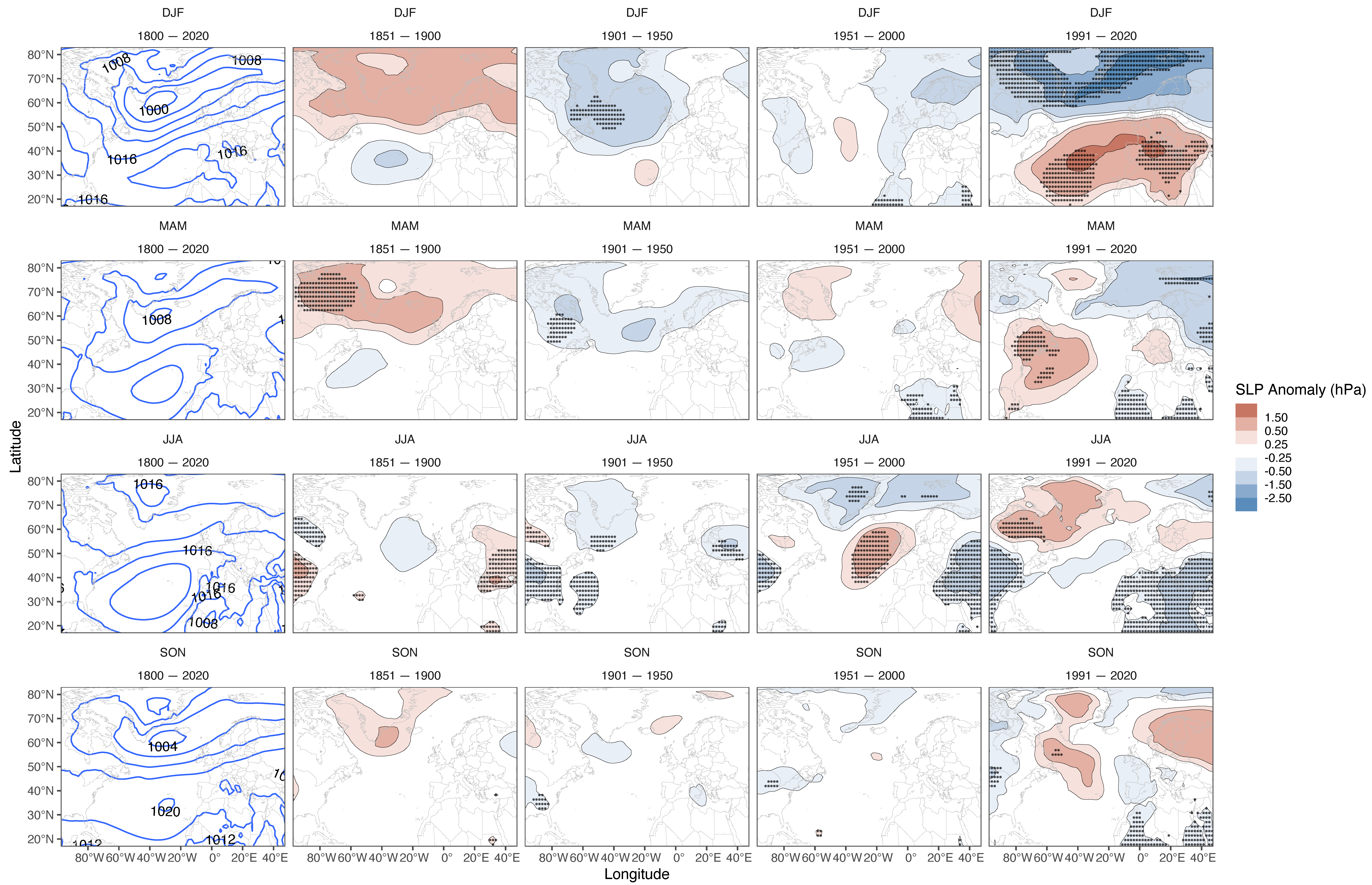
To maximise temporal consistency of the NAO and GBI time series over the whole time period, we spliced EKF400v2 and ERA5 mean sea-level pressure (NAO) and geopotential height (GBI) monthly datasets (i.e., adjusted the mean and standard deviation for the respective month so that they matched) against each other for the common EKF400v2/ERA5 overlap period of 1950–2003, before aggregating these monthly time series to seasonal before our analysis. Seasonal mean conditions and spatial anomalies of the patterns of 500 hPa geopotential height over the Greenland region and of North Atlantic mean sea-level pressure for different periods based on our spliced series are shown in Figure 1 and Figure 2.

We use three versions of the NAO in this study to account for potential differences between methodologies and underlying data. The first NAO, hereafter NAO_Fixed, represents a pseudo-station NAO using EKF400v2 and ERA5 sea level pressure from the reanalysis grid boxes encompassing Ponta Delgada, Azores and Reykjavik, Iceland. The Azores and Iceland time series are used to create the NAO for all 30 ensemble members of the spliced EKF400v2–ERA5 reanalysis. Both the Azores and Iceland MSLP seasonal time series are normalised using their respective means and standard deviations for 1951 to 2000 before the Iceland series is subtracted from the Azores. The Azores–Icelandic NAO is thought to better capture the annual migration of the NAO centres of action than using a continental southern station such as Lisbon or Gibraltar [5] (however, a British Isles–Greenland dipole is often identified as a more reflective Summer NAO spatial pattern [71]).

To better capture the summer NAO pattern, the second NAO, hereafter NAO_PC, uses the first principal component of detrended, monthly (aggregated to seasonal) SLP anomalies from the spliced EKF400v2–ERA5 dataset (1800–2020, anomalies using 1961–1990) covering −90° W–40° E, 20° N–80° N. We construct the NAO_PC from individual ensemble members, then average the time series (inverting the time series if necessary so the Azores dipole, or British dipole during summer, is the positive one). The explained variance varies for each ensemble member, but the mean across all ensemble members (i.e., NAO_PC) explains 34% (DJF), 32% (MAM), 30% (JJA) and 26% (SON) of the underlying SLP variability. NAO_Fixed and NAO_PC are generally well correlated but less strongly, and occasionally insignificantly, in summer compared with winter (Table S2), which reflects seasonal shifts in the NAO centres of action [71].

The final NAO, hereafter NAO_Luter [72] is used as a benchmark for comparing our 1800–1850 NAO_Fixed and NAO_PC values. NAO_Luter is an Azores–Iceland NAO series that was built based on proxy predictors from Eurasian instrumental (air pressure, precipitation and temperature) and documentary (cloud cover, snow and sea ice and phenological observations) sources. It is the only available (partly) instrumental-based Azores–Iceland record that extends before 1850, and provides a useful cross-reference in our evaluation of NAO seasonal values during 1800–1830 that may have been influenced by the 1815 Tambora volcanic eruption and/or the Dalton solar minimum.

For GBI, we use two measures, where GB₁ is simply the normalised area-weighted 500 hPa geopotential height over the region 60–80° N, 20–80° W [17,18] and GB₂ is the area-weighted 500 hPa geopotential height over this Greenland region minus that calculated over the entire hemispheric zonal band of 60–80° N [34]. GB₂ is sometimes preferred to mitigate the possible effect of global warming on mean height levels, as discussed in Section 1. GB₁ and GB₂ are very highly correlated for all seasons and periods (Table S3). We normalise GB₁ and GB₂ values using the 1951–2000 period.

2.4. Statistical Analyses

We use a 21-point binomial filter to emphasize long-term decadal variability in GBI and NAO. Following Hanna et al. (2015), we also use an 11-year running standard deviation to examine potential long-term changes in GBI/NAO year-to-year variability. We use standard significance testing of linear trends, ascribing significance to results where p ≤ 0.05. Standard three-month meteorological seasons are used, where winter (DJF) corresponds to the year marked by the January. To evaluate statistical properties of our new NAO and GBI time series, we evaluate various periods throughout the series but with a focus on two recent periods 2000–2020 and 2007–2020, which mark the recent era of strong Arctic warming and, especially, the record run of low Arctic sea ice summers since 2007 (using two recent periods allows us to assess the time sensitivity of our results). We use the hypergeometric distribution to identify the significance of 21st century NAO and GBI record high/low events, as in [7] following [73]. The hypergeometric distribution is a discrete probability distribution describing the probability of k successes (random draws for which the object drawn has a specified feature) in n draws, without replacement (and is therefore different from the binomial distribution), from a finite population containing K objects with that feature, in which each draw is either a success or a failure. For example, in an N-year record for a particular season, we define 10 record years (extreme high and low GBI or NAO values), N-10 non-record years and 21 years (2000–2020) as sampling “draws”. Due to testing multiple seasons and extreme value types (both high and low values), Bonferroni corrections (×8 scaling) are applied to reported p-values to mitigate the increased likelihood of rejecting the null hypothesis of no significant clustering of extreme GBI or NAO seasonal values in the last ~20 years of record.

3. Results

3.1. Key Features of 1800–2020 GBI/NAO Series

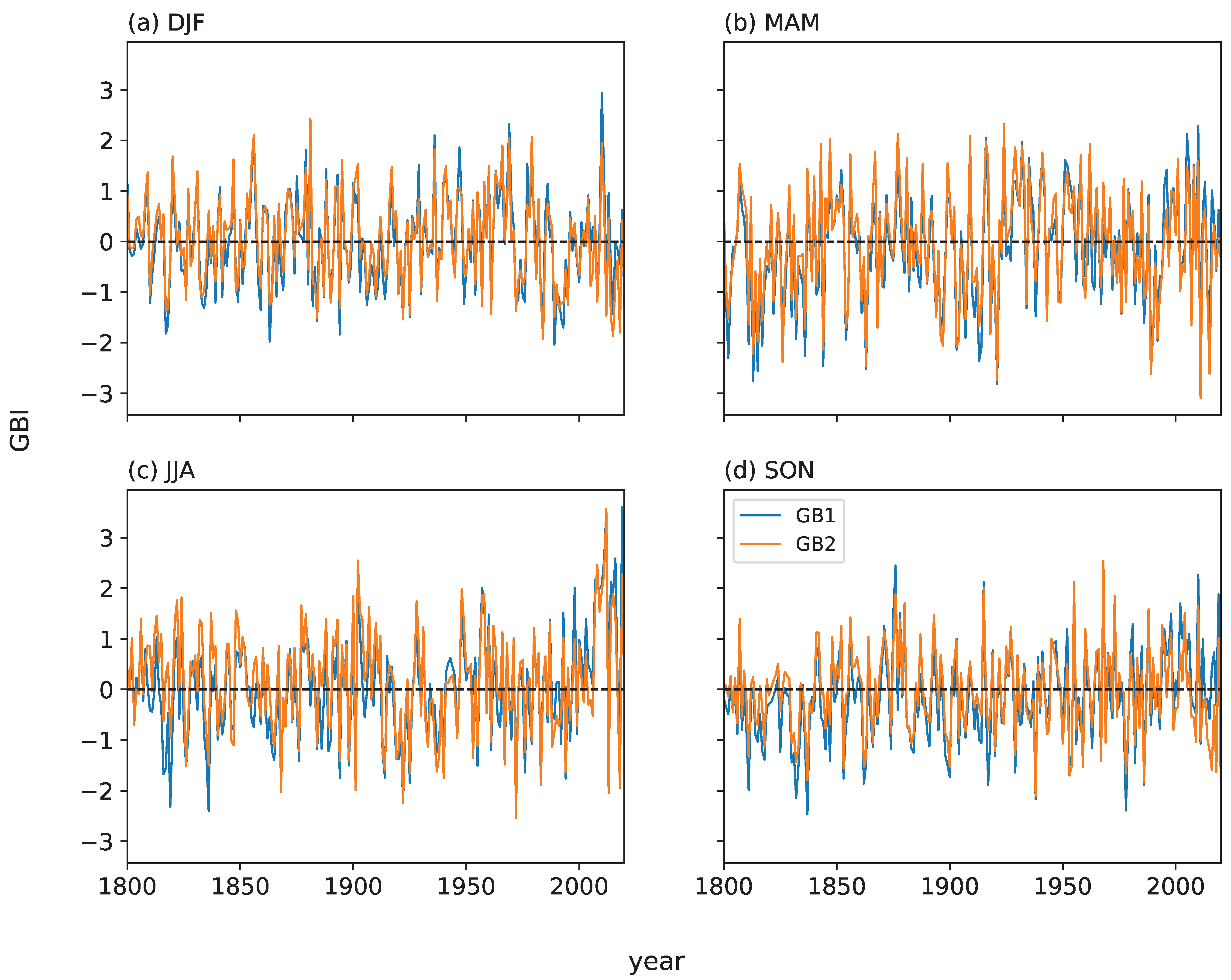
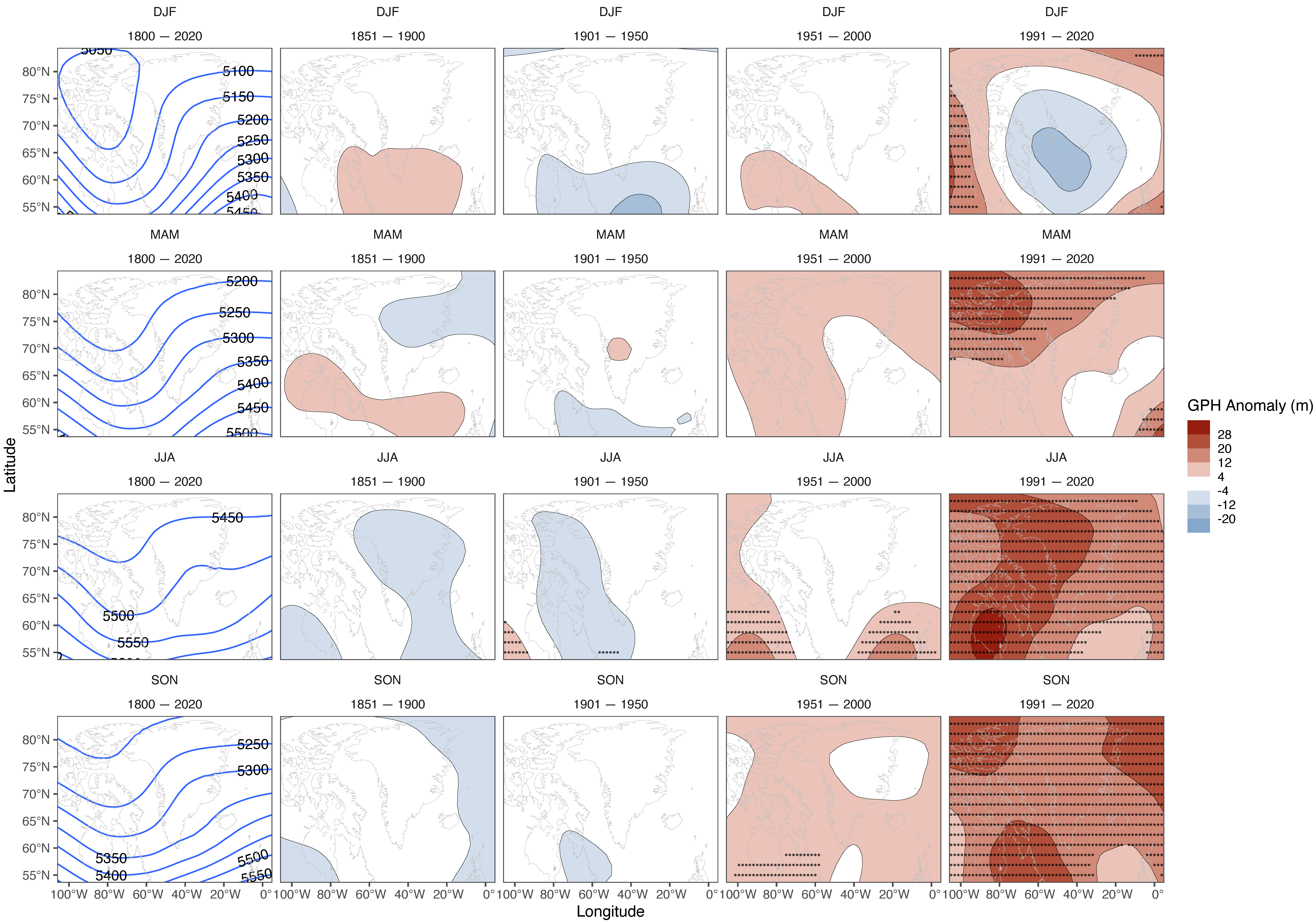
The winter seasonal time series of normalised GB₁ for the full period of records shows a record peak (2.94 standard deviations above the 1951–2000 winter mean) in 2010 (Figure 3a). However, in the winter GB₂ series, 2010 is only the fifth highest value, while the three lowest values are in 1984, 2015 and 2018, in contrast to a more even distribution of extreme low values over time in the GB₁ series (Figure 3a). Despite these differences, there is no obvious overall trend in winter GB₁ or GB₂ values or variability over the whole period of records. However, the spatial geopotential height plots show moderate negative anomalies centred over southern and central Greenland, surrounded by moderate positive anomalies, for winter for the 1991–2020 period, with these mostly non-significant anomalies cancelling the wider GBI region (Figure 1). For spring, GB₁ shows the highest value in 2010, while GB₂ has its lowest value in 2011, but again there is no clear long-term trend or overall change in variability with time (Figure 3b). Spatial anomalies for 1991–2020 for spring are significantly positive and greatest over northwest Greenland and towards the Canadian Arctic (Figure 1), which may reflect greater heating of the near-surface atmosphere from seasonally reduced sea ice cover. The summer GBI graph shows several highly unusual high values since 2007 and extreme year-to-year fluctuations between successive summer seasons, i.e., 2012 (high GBI)–2013 (low GBI) and 2018 (low GBI)–2019 (high GBI) (Figure 3c). These two recent summer pairs have by far the highest such interannual fluctuations in the entire period of the GB₁ record, and two of the three greatest year-to-year fluctuations in the GB₂ record. The overall increase in summer GBI in the last few decades is reflected by the 1991–2020 spatial anomaly map (Figure 1), which shows significantly high geopotential height anomalies over the whole of Greenland and its immediate surroundings but are greatest in west and northwest Greenland and in the Davis Strait. Autumn has the highest (lowest) GB₁ value in 1876 (1837) and the highest (lowest) GB₂ value in 1968 (1938) with no clear pattern in the temporal distribution of extreme values (Figure 3d). An underlying increase in autumn GBI from the late 1970s to the mid-2000s (also shown as significant positive anomalies from 1991–2020 in Figure 1), following a slight decrease since the mid-nineteenth century, generally reversed in the last 15 years of the records. The most frequent categories of GB₁ values (i.e., the numbers of years with mean GBI values for the respective period) shifted in summer from GB₁ < −0.5 during all the 50-year periods to 2000, to >0.5 in 2000–2020 and >0.5 and >1 (joint equal) in 2007–2020 (Figure 4). The only mean summer GB₁ values exceeding one standard deviation (with the year-to-year standard deviation for the respective period shown in brackets) were 1.35 (1.28σ) for 2000–2020 and 1.74 (1.38σ) for 2007–2020 (Figure 4). This pattern of a recent moderate increase in summer GBI is confirmed using GB₂ in Table S4, which suggests that the increase is not solely due to thermodynamics and there is a circulation component. There are no clear overall changes for the other seasons.

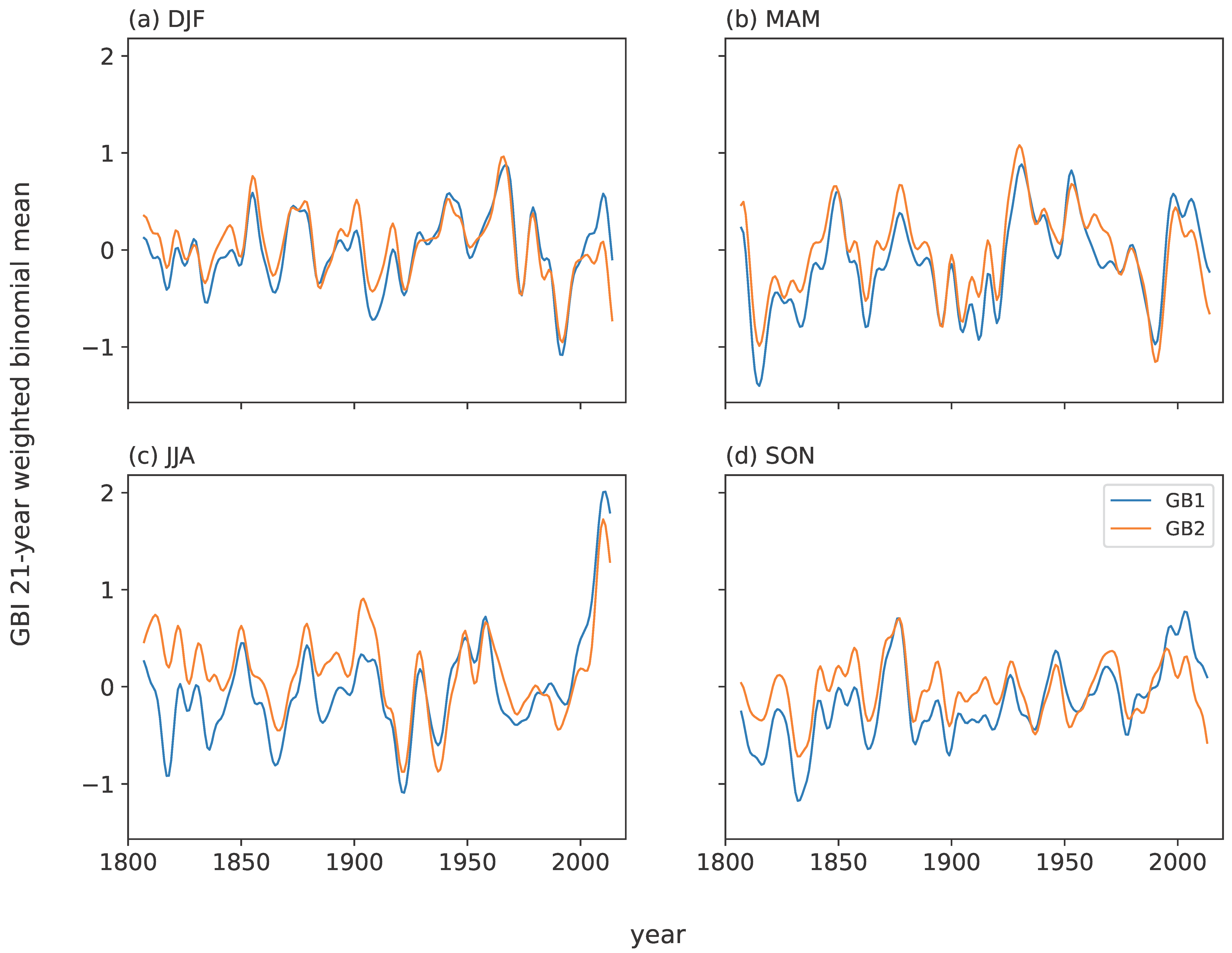
Smoothed series of seasonal GBI (Figure 5) show major peaks in the mid–late 1960s for winter and around 2010 for summer. The recent summer increase is statistically significant since 1951 in GB₁ but not GB₂ (

Table 1. Mean correlation coefficients (R) and number of ensemble members with significant trends (n), based on individual analysis of all 30 ensemble members of EKF400v2 (1800–1949) spliced with ERA5 (1950–2020), of trends in GBI and NAO for the entire records and various sub-periods. n shows the number of ensemble members with significant trends (for the pre-ERA5 period where ensemble members are used). Significant upward (downward) temporal overall trends, determined based on reference [74], with the corresponding number of significant ensemble trends, are emboldened in red (blue).

Parameter	DJF		MAM		JJA		SON
	R	n	R	n	R	N	R	n
GB1
1800–2020	0.045	0	0.155	18	0.220	29	0.219	26
1851–2020	0.036	0	0.087	5	0.271	28	0.148	15
1901–2020	0.037	0	0.092	1	0.325	30	0.198	20
1951–2020	0.163		0.080		0.376		0.180
1991–2020	0.224		0.004		0.481		0.091
GB2
1800–2020	0.109	9	0.045	0	0.049	1	0.053	2
1851–2020	0.149	13	0.050	0	0.085	3	0.093	7
1901–2020	0.159	11	0.075	0	0.131	6	0.068	3
1951–2020	0.309		0.233		0.187		0.101
1991–2020	0.018		0.052		0.312		0.435
NAOFixed
1800–2020	0.126	12	0.063	1	0.093	11	0.080	4
1851–2020	0.146	16	0.080	2	0.056	0	0.096	8
1901–2020	0.103	3	0.057	0	0.064	0	0.061	0
1951–2020	0.299		0.162		0.186		0.024
1991–2020	0.118		0.025		0.139		0.177
NAOPC
1800–2020	0.006	0	0.004	0	0.010	0	0.007	0
1851–2020	0.066	0	0.080	2	0.067	0	0.056	1
1901–2020	0.075	0	0.058	0	0.077	0	0.051	0
1951–2020	0.292		0.286		0.180		0.087
1991–2020	0.020		0.176		0.241		0.330

). Peak spring GBI values occur around 1930, which is most pronounced for GB₂. Autumn values are relatively high around the late 1870s and early 2000s (GB₁ only). Low points are seen around 1990 for winter and spring, the early 1920s and (GB₂) late 1930s for summer and 1832 for autumn. Peaks in interannual variability in GBI are shown for winter, and especially for spring and summer, in the last decade of the record (Figure 6). However, linear trends (associated with these recent peaks and other fluctuations) of the overall GB₁/GB₂ variability time series and selected sub-series are mostly not statistically significant, except for a significant increase in GB₂ variability for spring during 1951–2015 (

Table 2. Mean correlation coefficients (R) and number of ensemble members with significant trends (n), based on individual analysis of all 30 ensemble members of EKF400v2 (1800–1949) spliced with ERA5 (1950–2020), of trends in 11-year running standard deviation of GBI and NAO for the entire records and various sub-periods. Other details are as stated in the Table 1 caption. In assessing statistical significance, degrees of freedom were scaled by the smoothing interval (i.e., number of years minus two were divided by eleven). Significant upward temporal overall trends, determined based on reference [74], with the corre-sponding number of significant ensemble trends, are emboldened in red.

Parameter	DJF		MAM		JJA		SON
	R	n	R	n	R	n	R	n
GB1runsd11yr
1800–2015	0.099	0	0.148	0	0.133	0	0.202	1
1851–2015	0.152	0	0.093	0	0.204	1	0.170	1
1901–2015	0.341	0	0.191	0	0.216	0	0.122	0
1951–2015	0.124		0.666		0.483		0.372
GB2runsd11yr
1800–2015	0.110	0	0.143	0	0.105	0	0.161	0
1851–2015	0.101	0	0.107	0	0.119	0	0.216	1
1901–2015	0.202	0	0.189	0	0.096	0	0.175	0
1951–2015	0.141		0.757		0.312		0.638
NAOFixedrunsd11yr
1800–2015	0.295	2	0.118	0	0.174	1	0.105	0
1851–2015	0.281	0	0.108	0	0.129	0	0.141	0
1901–2015	0.494	0	0.179	0	0.268	0	0.090	0
1951–2015	0.528		0.831		0.275		0.184
NAOPCrunsd11yr
1805–2015	0.335	7	0.114	0	0.103	0	0.239	3
1851–2015	0.332	1	0.117	0	0.283	0	0.211	1
1901–2015	0.745	30	0.068	0	0.176	0	0.263	0
1951–2015	0.692		0.691		0.157		0.242

). Eight (six) of the ten highest GB₁ (GB₂) summer values in the entire record have occurred since 2000 (

Table 3. Ten highest and ten lowest GB₁ and GB₂ years/values for each season for 1800–2020. Years since 2000 inclusive are emboldened, and these years are also shaded where they feature in both GB metrics.

DJF
GB1	GB1	GB2	GB2
High	Low	High	low
2010/2.94	1989/−2.04	1881/2.43	1984/−1.92
1969/2.32	1863/−1.98	1856/2.11	2015/−1.87
1881/2.19	1894/−1.84	1979/2.07	2018/−1.80
1936/2.10	1817/−1.82	1969/2.04	1922/−1.54
1856/2.01	1993/−1.70	2010/1.95	1884/−1.52
1947/1.86	1818/−1.66	1966/1.90	1989/−1.50
1879/1.81	1884/−1.58	1936/1.82	2014/−1.49
1895/1.58	1922/−1.53	1847 and 1895/1.62	2012/−1.47
1977/1.54	1992/−1.52		1925/−1.45
1929/1.52	1925/−1.50	1855/1.58	1961/−1.43
MAM
GB1	GB1	GB2	GB2
High	Low	High	Low
2010/2.28	1921/−2.81	1924/2.32	2011/−3.10
2005/2.13	1813/−2.75	1877/2.13	1921/−2.74
1909/2.07	2011/−2.68	1909/2.09	1989/−2.62
1916/2.05	1815/−2.56	1847/2.02	2015/−2.61
1924/2.02	1863/−2.52	1916/1.98	1863/−2.47
1932/1.97	1844/−2.46	1843 and 1962/1.93	1826/−2.38
1843/1.78	1913/−2.37		1813/−2.22
1962/1.76	1802/−2.31	1932/1.89	1844/−2.14
1877/1.75	1836/−2.27	1929/1.86	1903/−2.08
1935/1.66	2015/−2.24	1867/1.78	1897/−2.06
JJA
GB1	GB1	GB2	GB2
High	Low	High	Low
2019/3.61	1836/−2.41	2012/3.57	1972/−2.54
2012/3.54	1819/−2.32	1902/2.55	1922/−2.24
2016/2.59	1922/−2.23	2008/2.46	2013/−2.05
2011/2.56	1972/−1.94	2019/2.28	1868/−2.02
2007/2.17	1925/−1.85	2011/2.27	1901/−1.99
2014/2.13	1868/−1.81	1948/1.98	2018/−1.94
2010/2.07	1994 and 1983/−1.76	2010/1.94	1983/−1.88
2008/2.03		1958 and 2015/1.88	1940/−1.75
1957 and 1998/2.01	1894/−1.75		1925/−1.65
	1914/−1.74	1957/1.85	1994/−1.64
SON
GB1	GB1	GB2	GB2
High	Low	High	Low
1876/2.45	1837/−2.47	1968/2.54	1938/−2.11
1968/2.41	1978/−2.39	1955/2.13	2020/−1.94
2010/2.27	1938/−2.17	1915/2.01	1986/−1.82
1915/2.12	1832/−2.15	1876/1.88	1837/−1.79
2019/1.88	1811/−1.99	1973/1.85	1953/−1.70
1955/1.75	1917 and 1986/−1.89	1880/1.71	1978/−1.66
2002/1.70		2010/1.65	2018/−1.63
1878/1.51	1862/−1.86	1988/1.59	2016/−1.59
1998/1.50	1853/−1.76	2004/1.51	1853/−1.55
1875/1.47	1900/−1.73	1893/1.47	1862/−1.54

). This is very highly significant (p ≤ 0.00045) according to the hypergeometric distribution, with a Bonferroni correction applied to the p-value to account for multiple sampling across four seasons and the two high/low extremes we sample for in Table 3. The top two GBI summers (combined GB₁ and GB₂ rankings) are 2012 and 2019, closely followed by 2011, 2008 and 2010. No similar (significant) recent clustering of extreme GBI years is seen for the other seasons. However, 2010 features in the ten highest GB₁ and GB₂ years for winter, spring (GB₁ only), summer and autumn, while 2018 is in the ten lowest winter and autumn GB₂ (but not GB₁) values, and 2013 has the third lowest summer GB₂ value.

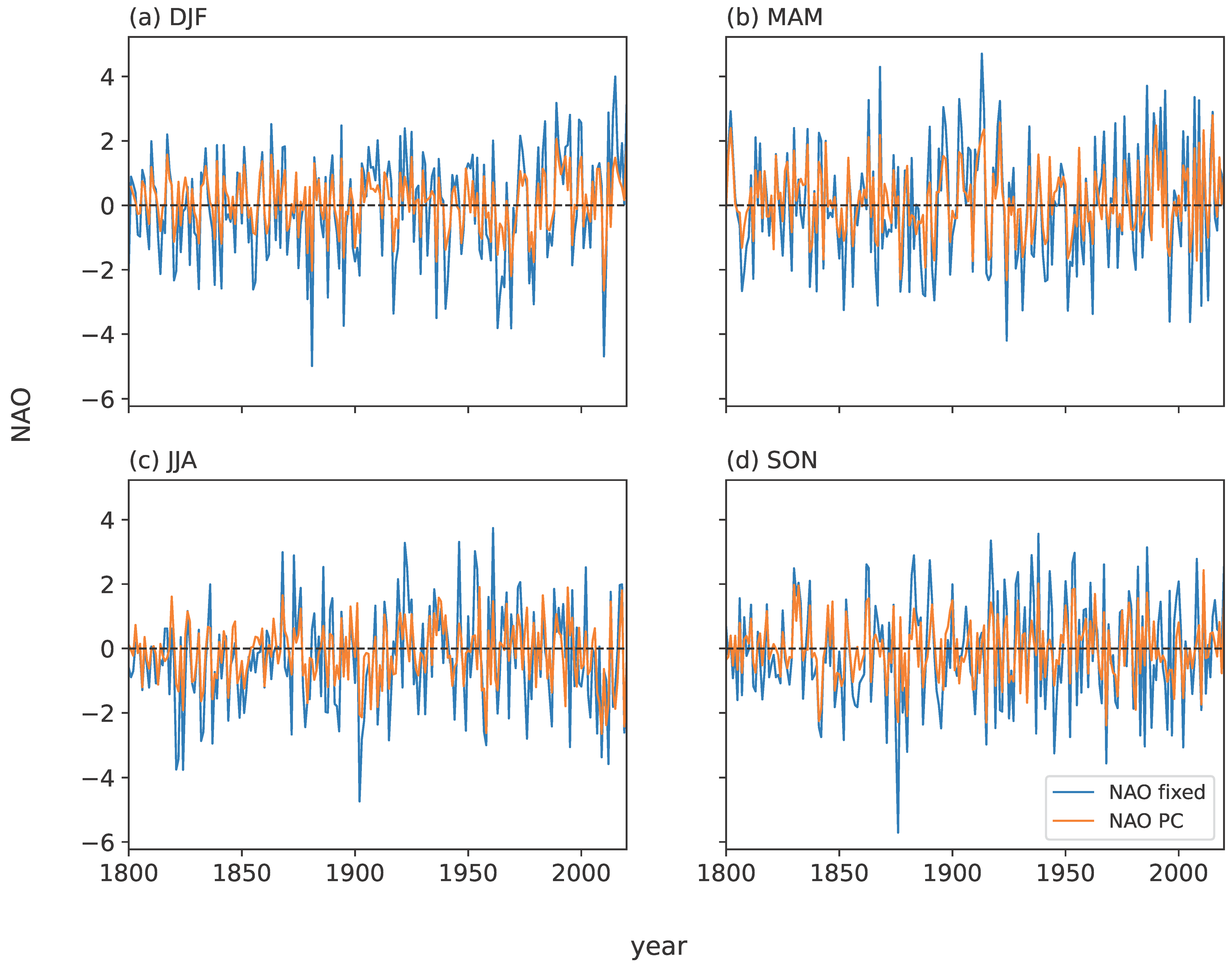
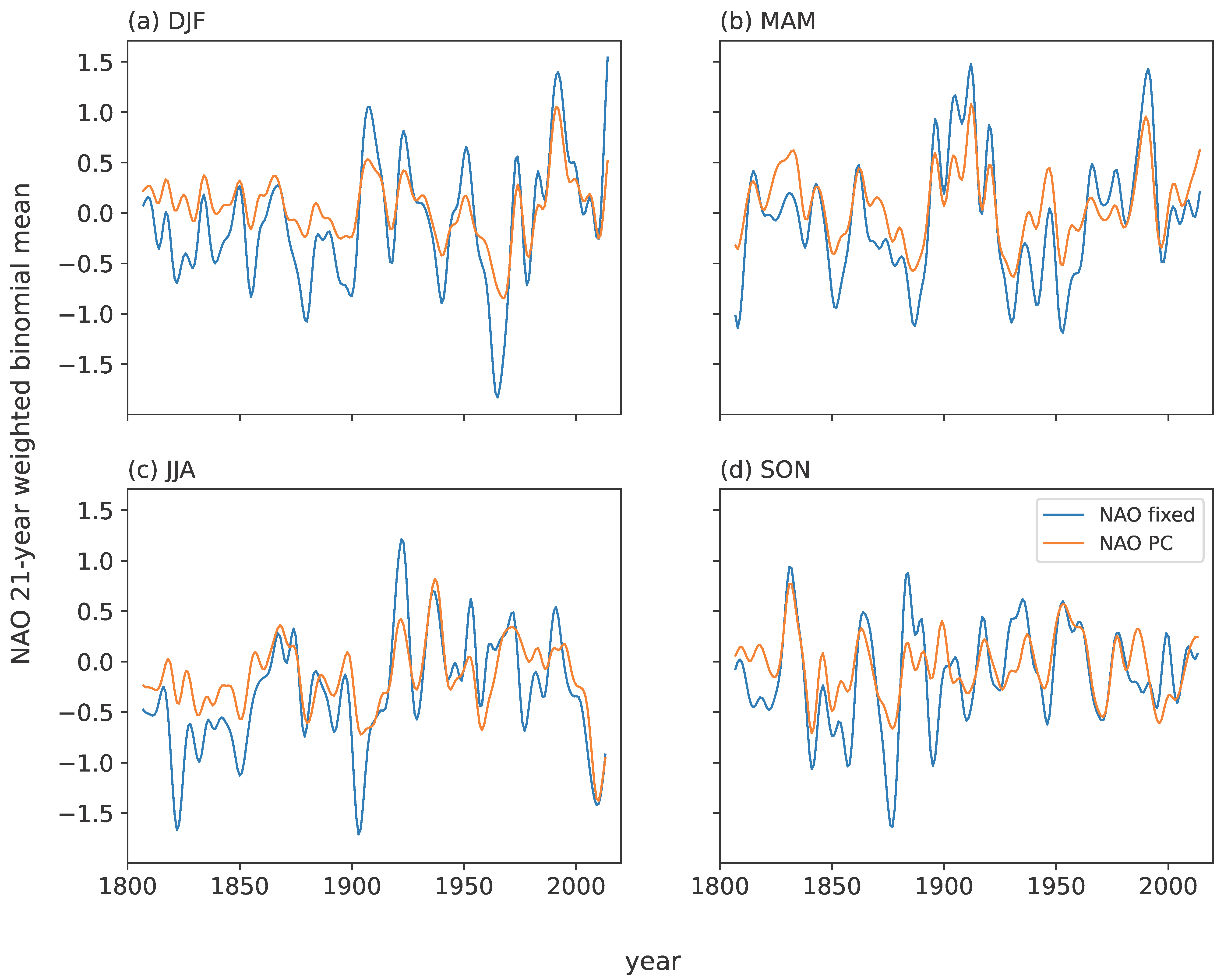
NAO seasonal data (Figure 7 and Figure 8) show no overall long-term trends in mean values but exhibit increased year-to-year variability in the last decade in winter (Figure 7a), but other seasons (Figure 7b–d) show the greatest variability at various points in the mid–late nineteenth century and early- or mid-twentieth century. The North Atlantic MSLP winter anomaly plot for 1991–2020 shows significant positive anomalies centred around the Azores and significant negative anomalies close to the north of Iceland (Figure 2), which reflect relatively positive NAO values overall during the last few decades of the record (Figure 7a). There are signs of a summer NAO decrease since about 1990 (Figure 7c and Figure 8), confirmed by the North Atlantic MSLP summer anomaly plot for 1991–2020 (Figure 2), which supplements the summer GB₁ increase and follows expectation based on the strong negative correlation between the NAO_PC and GB₁ series (

Table 4. Detrended correlation coefficients between seasonal GB₁ and NAO indices for various periods. Shaded values are *not* statistically significant at the p ≤ 0.05 level.

	Period	DJF	MAM	JJA	SON
GB1, NAOFixed	1801–1850	−0.87	−0.85	−0.79	−0.85
GB1, NAOFixed	1851–1900	−0.91	−0.74	−0.74	−0.80
GB1, NAOFixed	1901–1950	−0.84	−0.88	−0.81	−0.76
GB1, NAOFixed	1951–2000	−0.85	−0.75	−0.43	−0.72
GB1, NAOFixed	1951–1980	−0.88	−0.73	−0.47	−0.83
GB1, NAOFixed	1961–1990	−0.89	−0.73	−0.40	−0.80
GB1, NAOFixed	1971–2000	−0.82	−0.74	−0.32	−0.65
GB1, NAOFixed	1981–2010	−0.85	−0.85	−0.46	−0.67
GB1, NAOFixed	1991–2020	−0.89	−0.82	−0.66	−0.58
GB1, NAOPC	1801–1850	−0.89	−0.84	−0.82	−0.86
GB1, NAOPC	1851–1900	−0.95	−0.81	−0.84	−0.92
GB1, NAOPC	1901–1950	−0.91	−0.90	−0.90	−0.87
GB1, NAOPC	1951–2000	−0.93	−0.84	−0.85	−0.86
GB1, NAOPC	1951–1980	−0.94	−0.80	−0.88	−0.88
GB1, NAOPC	1961–1990	−0.95	−0.84	−0.84	−0.86
GB1, NAOPC	1971–2000	−0.93	−0.85	−0.84	−0.84
GB1, NAOPC	1981–2010	−0.93	−0.91	−0.82	−0.86
GB1, NAOPC	1991–2020	−0.93	−0.90	−0.89	−0.84

). Smoothed NAO seasonal series for winter show maxima in the mid-1900s to early-1920s and around 1990, and a deep minimum in the mid-1960s (Figure 9a). Spring has high (low) points around 1910 and 1990 (late 1880s, 1930 and early 1950s) (Figure 9b). Figure 9c shows summer maxima in the early 1920s or late 1930s and minima around 1900 and 2010 (also 1822 for NAO_Fixed). The two autumn NAO series do not always correspond well through time but have a common high (low) point in the early 1830s (late 1870s). Further analysis of NAO_PC shows a slight but insignificant shift to more positive (negative) winter (summer) values during the latest two periods since 2000 (Figure 8). Mean (year-to-year standard deviation) NAO_PC summer values are −0.73 (1.25σ) in 2000–2020 and −1.00 (1.41σ) in 2007–2020. The slight but overall insignificant summer NAO decrease (Figure 2) is mirrored using the NAO_Fixed values in Table S5.

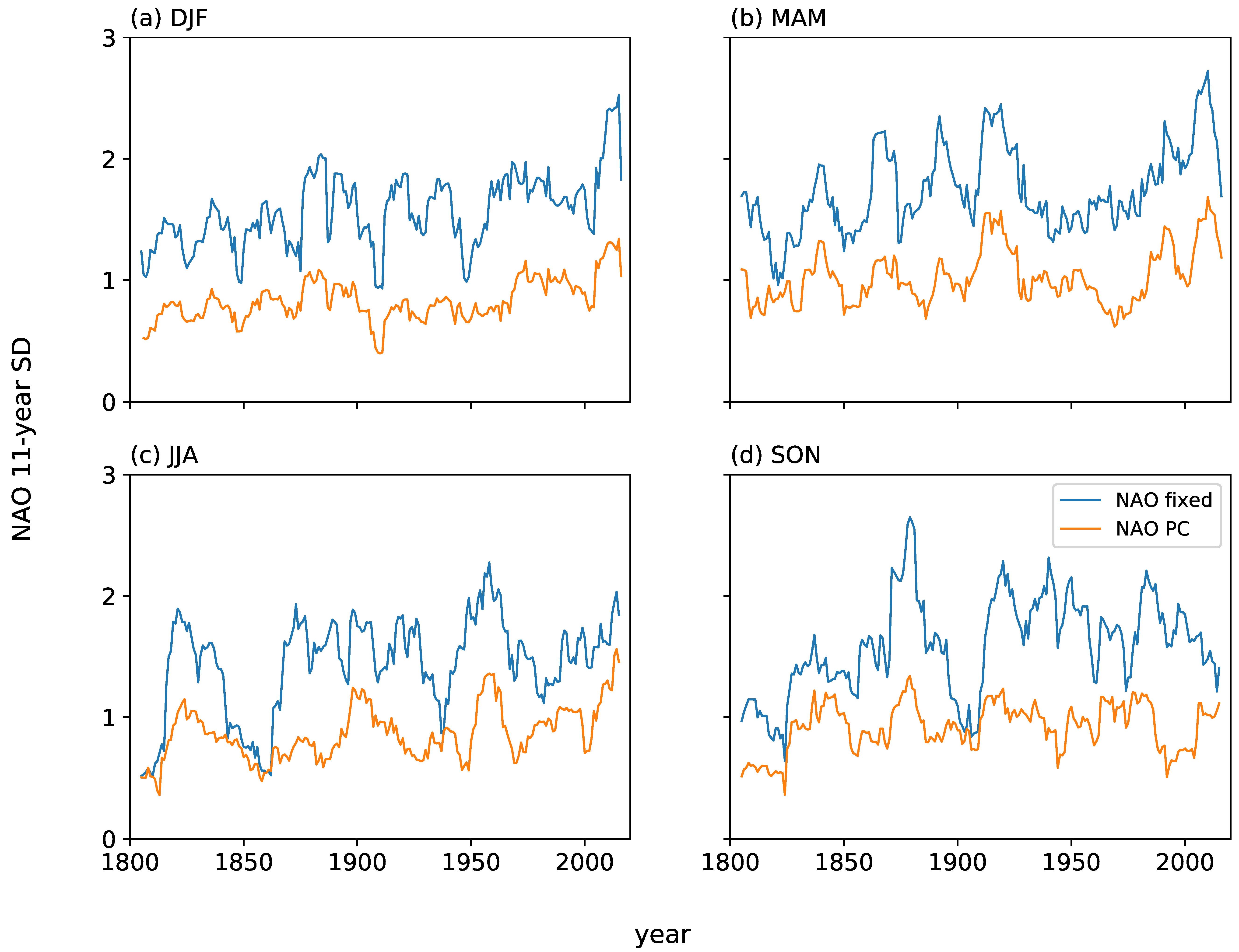
Interannual variability of NAO seasonal time series (Figure 10, Table 2) shows a significant increase in winter variability (p = 0.005) for NAO_PC during 1901–2015, although, due to the high degree of smoothing, the NAO_PC winter variability increase from 1951–2015 is not quite significant (p = 0.07). Increases in NAO_Fixed winter variability are not statistically significant, although NAO_Fixed does become significantly more variable in spring during 1951–2015 (p = 0.021). Secular changes in the year-to-year variability of winter NAO include lower variability around 1850, 1910, 1950 and 2005) (Figure 10a), while spring variability peaks around 1920 and then decreases during the mid-twentieth century before once again increasing to reach a similar or slightly greater peak in about 2010 (Figure 10b). Summer variability peaks around 1820, 1900 and in the late 1950s (Figure 10c). The recent peak (~2010) is slightly higher than the earlier summer peaks for the NAO_PC series and similar to or lower than the former peaks for the NAO_Fixed record.

Table 5. Ten highest and ten lowest NAO_Fixed and NAO_PC years/values for each season for the period 1800–2020. Years since 2000 inclusive are emboldened, and these years are also shaded where they feature in both GB metrics.

DJF
NAOFixed	NAOFixed	NAOPC	NAOPC
High	Low	High	Low
2015/4.00	1881/−4.99	1989/2.06	2010/−2.64
1989/3.18	2010/−4.69	2020/1.80	1969/−2.19
2020/3.10	1969/−3.82	1817/1.57	1881/−2.03
2012/2.88	1963/−3.81	1863/1.57	1979/−1.76
1995 and 2014/2.81	1895/−3.74	1993/1.52	1936/−1.74
	1936/−3.50	2000/1.50	1895/−1.62
1999/2.66	1917/−3.36	1925/1.50	1963/−1.53
1984/2.61	1940/−3.21	2015/1.48	1879/−1.48
2000/2.56	1979/−3.07	1995/1.48	1977/−1.43
1863/2.52	1879/−2.91	1884/1.45	1917/−1.43
MAM
NAOFixed	NAOFixed	NAOPC	NAOPC
High	Low	High	Low
1913/4.71	1924/−4.20	2015/2.79	1924/−2.32
1868/4.30	2005/−3.62	1921/2.57	1877/−2.29
1986/3.71	1996/−3.61	1990/2.48	1888/−1.93
1994/3.56	1962/−3.37	1802/2.39	1909/−1.73
2007/3.36	1951/−3.27	1914/2.36	2008/−1.71
1903/3.30	1931/−3.26	2011/2.33	1892/−1.71
1863/3.27	1852/−3.25	1868/2.18	1916/−1.69
2009/3.26	2010/−3.12	1913/2.17	1843/−1.68
1921/3.24	1867/−3.11	1863/2.12	1951/−1.65
1896/3.05	1892 and 2013/−2.59	1844/1.95	1931/−1.61
JJA
NAOFixed	NAOFixed	NAOPC	NAOPC
High	Low	High	Low
1961/3.74	1902/−4.74	1955/1.91	2009/−2.65
1946/3.31	1824/−3.76	1994/1.89	1958/−2.62
1922/3.28	1821/−3.75	2018/1.80	2019/−2.42
1953/3.02	2012/−3.58	1868/1.65	2011/−2.38
1868/2.99	1822/−3.42	1983/1.65	1903/−2.13
1873/2.89	2009/−3.37	1819/1.61	1902/−2.05
1886 and 1923/2.53	1995/−3.06	1937/1.58	1824/−1.92
	1958/−3.00	1961/1.46	1907/−1.89
2002/2.52	1837/−2.95	1938/1.46	2015/−1.87
1954/2.47	1832/−2.87	2013/1.45	1910/−1.81
SON
NAOFixed	NAOFixed	NAOPC	NAOPC
High	Low	High	Low
1938/3.56	1876/−5.71	2011/2.43	1968/−2.38
1917/3.35	1968/−3.56	1938/2.02	1915/−2.30
1986/3.14	1945/−3.25	1830/1.97	1876/−2.28
1954/2.97	1880/−3.21	1832/1.95	1841/−2.25
1935/2.90	2002/−3.07	1954/1.85	1880/−2.09
1883/2.89	1985/−3.04	1953/1.82	1981/−1.90
2008/2.78	1915/−2.98	1986/1.73	1842/−1.86
1890/2.74	1871/−2.93	1963/1.69	2010/−1.74
1953/2.65	1852/−2.84	1982/1.56	1933/−1.68
1862 and 1967/2.61	1842 and 1952/−2.75	1863/1.56	1998/−1.57

confirms the unusual atmospheric circulation pattern in winters 2010 (which was the most negative NAO_PC and second most negative NAO_Fixed winter on record) and 2015 (the most positive NAO_Fixed and eighth most positive NAO_PC winter). Five recent winters (2000, 2012, 2014, 2015 and 2020) feature in the top ten NAO_Fixed values, with three of these years (2000, 2015 and 2020) in the NAO_PC top ten winters. Given the overall length of record, five record values is a significant clustering based on the Bonferroni-corrected hypergeometric distribution (adjusted p = 0.0068). Since both our extended NAO records also include 2010 as a record low NAO winter, this can alternatively be tested as a cluster of either four or six of the most extreme NAO winters values having occurred in the last 21 years, which is also a significant clustering in the NAO_Fixed winter series (adjusted p = 0.040). The year 2009 features in the lowest summer values in both NAO indices, while the NAO_PC summer index has four recent years (2009, 2011, 2015 and 2019) in its lowest ten values, which is not quite statistically significant (adjusted p = 0.064). In addition, 2012, the fourth lowest NAO_Fixed summer value, forms part of the major recent cluster of high GBI summers and is dynamically linked through concomitant changes in the North Atlantic polar jet stream (Hanna et al. 2018a).

Detrended correlation coefficients between GB₁ and the two NAO indices are summarised in Table 4. These are nearly all significant and are strongest in winter and weaker in summer. Correlations are generally higher using NAO_PC index, while GB₁–NAO_Fixed location correlations in summer are insignificant for 1971–2000. There are no clear long-term trends or variations in these correlations, except for weaker summer GBI and NAO_Fixed values clustered in the mid–late twentieth century. Our combined results suggest this may reflect changing centres of action of the NAO during this period rather than a weaker influence of Greenland Blocking on the NAO.

3.2. Evaluation of NAO and GBI Values from 1800–1830

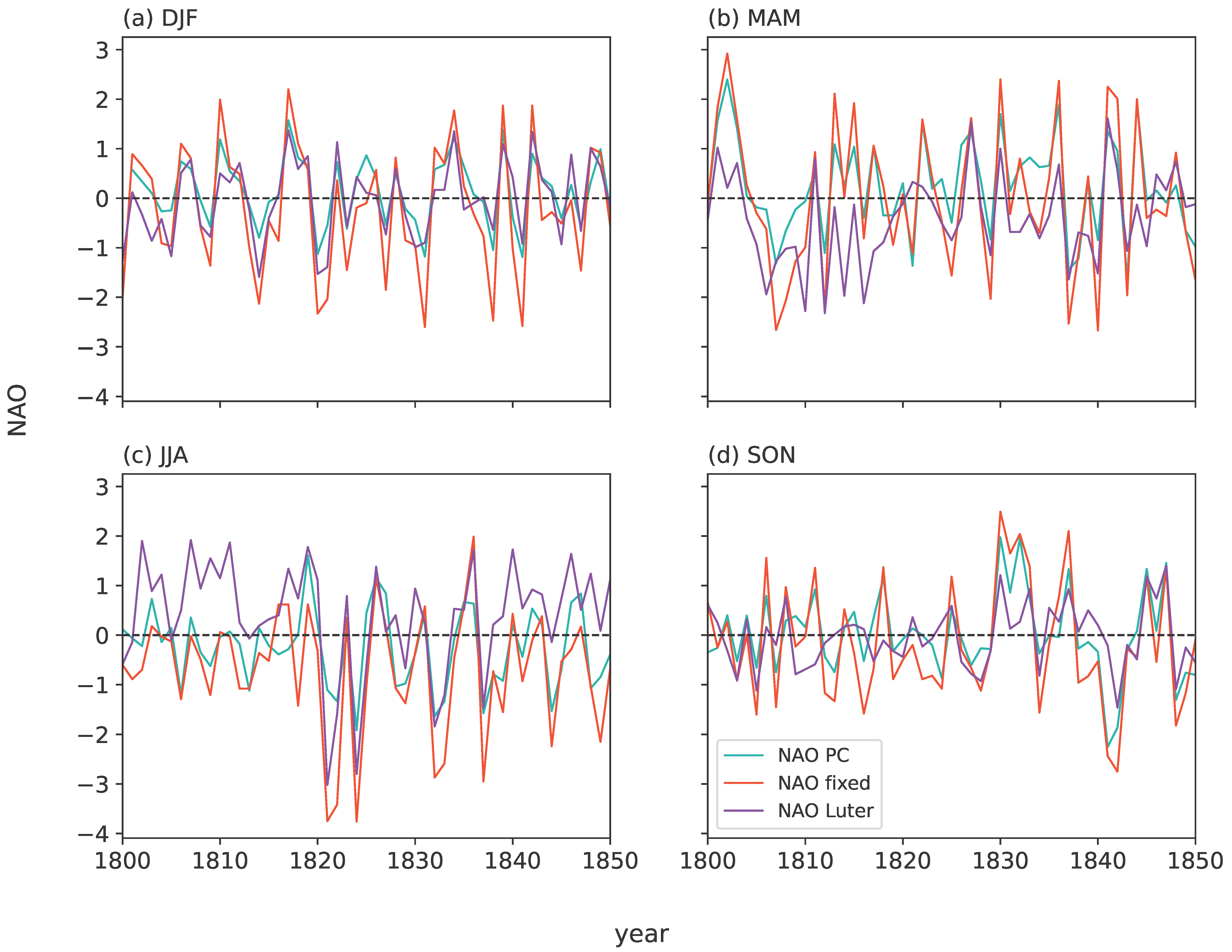
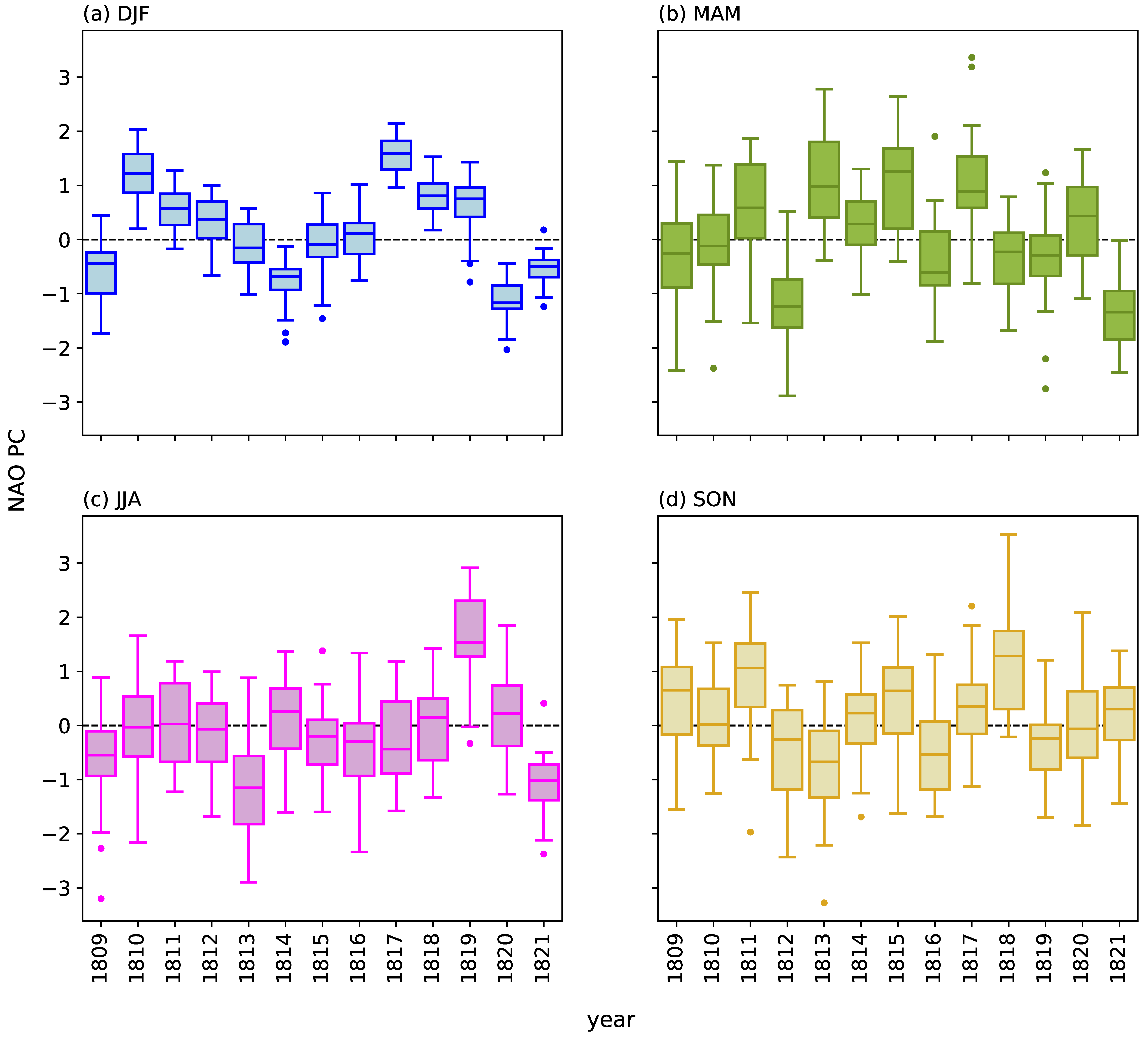
This period is of particular interest because it coincides with the Dalton solar minimum as well as the 1815 Tambora volcanic eruption. We therefore next examine summary statistics of NAO and GBI annual values and their variations. Figure 11 shows variations in NAO based on our NAO_PC and NAO_Fixed reconstructions and NAO_Luter. Our NAO series derived from EKF400v2 are significantly correlated with NAO_Luter for all seasons, with the strongest correlations for winter and when using NAO_Fixed rather than NAO_PC for the other three seasons (

Table 6. Correlation coefficients between our seasonal NAO_PC and NAO_Fixed indices and Luterbacher et al. (2002) NAO (NAO_Luter) for 1800–1830 and 1800–1850. All values are significant at the p ≤ 0.05 level.

NAO index pair	Period	DJF	MAM	JJA	SON
NAOLuter, NAOPC	1800–1830	0.89	0.62	0.57	0.39
NAOLuter, NAOPC	1800–1850	0.84	0.59	0.61	0.58
NAOLuter, NAOFixed	1800–1830	0.85	0.67	0.80	0.53
NAOLuter, NAOFixed	1800–1850	0.83	0.69	0.79	0.63

). EKF400v2 ensemble mean seasonal NAO mean values and their interannual variability for 1801–1830, together with yearly seasonal values for 1815–1817 (coincident with the immediate aftermath of Tambora) and their variability across ensemble members of EKF400v2, are shown in

Table 7. Summary statistics: (top) EKF400v2 ensemble means with interannual standard deviations of these means in brackets for 1800–1830; (lower) 1815–1817 annual seasonal values of respective NAO indices with ±values for NAO_Fixed and NAO_PC expressing ensemble standard deviation of all 30 EKF400v2 ensemble members. Annual seasonal values or means exceeding ±1σ are emboldened.

NAO index	DJF	MAM	JJA	SON
1801–1830
NAOFixed	−0.18 (1.20)	0.06 (1.50)	−0.69 (1.21)	−0.22 (1.03)
NAOPC	0.16 (0.63)	0.29 (0.96)	−0.19 (0.76)	0.05 (0.63)
NAOLuter	−0.04 (0.82)	−0.64 (1.02)	0.35 (1.29)	−0.11 (0.52)
1815
NAOFixed	−0.46 ± 1.15	1.93 ± 1.67	−0.52 ± 1.60	−0.36 ± 1.54
NAOPC	−0.07 ± 0.55	1.04 ± 0.90	−0.22 ± 0.70	0.46 ± 0.90
NAOLuter	−0.40	−0.13	0.32	0.21
1816
NAOFixed	−0.86 ± 1.07	−0.81 ± 1.40	0.62 ± 1.73	−1.58 ± 1.15
NAOPC	0.04 ± 0.41	−0.39 ± 0.82	−0.39 ± 0.78	−0.52 ± 0.78
NAOLuter	0.08	−2.12	0.40	0.12
1817
NAOFixed	2.20 ± 0.79	1.06 ± 1.10	0.62 ± 1.48	−0.68 ± 1.30
NAOPC	1.57 ± 0.32	1.05 ± 0.89	−0.29 ± 0.78	0.34 ± 0.74
NAOLuter	1.37	−1.07	1.34	−0.53

. Winters 1815 and 1816 have slightly negative or near-neutral NAO conditions; however, 1817 is the most positive value from the beginning (1800) of both EKF400v2-based NAO winter series until after 1850, with good agreement between the respective NAO indices (Figure 11a, Table 7). Box and whisker plots showing the spread of estimates between EKF400v2 ensemble members confirm a clear shift to a highly positive NAO in winter 1817 (Figure 11a). This is in agreement with the tendency for a major tropical volcanic eruption, such as Tambora, to favour a positive winter NAO [50], and this potential driver may have been augmented by solar activity being near the peak of the 11-year sunspot cycle in 1816 [75], although sunspot activity was then only midrange relative to a generally more active 11-year cycle outside the Dalton Minimum regime. A negative and then positive winter NAO in successive years following Tambora is in agreement with Reference [51]. Our results also show a similar positive NAO excursion in winter 1810, following another major volcanic eruption of unknown location in 1809, which was the third largest such event since 1500 with double the sulphur emission of the 1991 Pinatubo eruption [76] (Figure 11a and Figure 12a).

Summer and autumn NAO values for 1815–1817 are not far from neutral, with the possible exceptions of summer 1817, which NAO_Luter suggests was highly positive, and autumn 1816, which was strongly negative in NAO_Fixed but not in the other two indices (Figure 11c). The NAO_PC summer series indicates little apparent response to either the 1809 (unknown source) or Tambora 1815 volcanic eruptions. Available land-station pressure records and ships’ logs indicate a weak Azores High and strong Icelandic Low regime in summer 1816 (the infamous “year without a summer” (e.g., [77])), with low pressure anomalies focused over the UK [50] and cyclonic north-westerly flow giving anomalously wet and cool conditions both there ([78], pp. 339–340) and over central Europe; however, due to wider changes in the Euro–Atlantic pressure field, this circulation pattern might well correspond to a near-neutral rather than negative NAO, as indicated by [72]. Although fixed-location NAO indices can have problems capturing summer NAO changes (e.g., [2]), a near-neutral summer 1816 NAO value is suggested by all three NAO indices used in our study, including NAO_PC, which is not affected by this potential issue. Moreover, summers 1821, 1822 and 1824 are noteworthy as they are highly negative in all three NAO series that we use (Figure 11c). On the basis of the prevalence of sulfate fallout in ice cores in Antarctica and Greenland [79], the Tambora dust veil seems unlikely to have persisted into 1821. However, reference ([78], pp. 340–342) notes observations of notable coloured sunsets and twilights in London in summer 1821, attributing these to a volcanic dust veil effect, and confirms the impact of the highly negative summer NAO of 1821 on that year’s “very cool summer” in the British Isles.

During 1800–1830 (coincident with most of the Dalton Minimum), winter mean NAO values from the three available indices are on average near-neutral (Table 7), and there are a few moderate but unexceptional negative winter NAO excursions during this period (Figure 7a and Figure 11a). Although there is significant ensemble variability in EKF400v2 estimates of NAO for this period, clear differences between some consecutive years are still apparent (Figure 12), and the significant correlation with NAO_Luter values (Table 6) increases confidence in the EKF400v2 central estimates. Although there are no independent data that can help verify reanalysis estimates of Greenland Blocking for this period, our analysis suggests a number of negatively blocked (cyclonic Greenland) seasons during 1815–1817, i.e., winter 1817 GB₁ (GB₂) of −1.82 (−1.38), linked with the previously mentioned highly positive NAO, and a similar lack of blocking during the subsequent winter 1818 and in winter 1810; springs 1815 and 1817 were highly cyclonic, summer 1816 was moderately to strongly cyclonic, while autumns 1815 to 1818 were also cyclonic over Greenland.

4. Conclusions

We have presented newly developed Greenland Blocking and NAO indices based on recently released climate reanalyses, that exceed the span of previous similar records by 34% (221/165 years), including an insightful extension for much of the first few decades of the nineteenth century. Using the individual (n = 30) ensemble members to help assess trends has enabled us to overcome a major statistical limitation of using archived ensemble mean data. Our analysis confirms and extends (based on a longer record) previous results regarding a significant long-term increase in the year-to-year variability of the winter NAO_PC, which was previously highlighted for 1899–2014 for the month of December by [7], and here culminates in a significant clustering of extreme low/high values during 2000–2020 in our NAO_Fixed series. Whilst detailed physical interpretation is beyond the scope of this paper, we surmise that multiple factors acting on the winter polar jet to move it alternatively north and south appear to have been particularly active in recent decades: these factors are likely to include Arctic sea ice depletion and the recent deep solar minimum of ~2010 related to the downturn in the ~80-year solar cycle, as well as changes in North Atlantic sea-surface temperature patterns, tropical convection and ENSO [11,13,16]. Increased year-to-year variability of NAO in recent decades has important implications for seasonal–decadal weather prediction and severe weather planning, especially if these trends continue. The interannual variability increase in winter, with a simultaneously, positively-biased NAO in the future could both be sustained if meteorologically extreme events such as the 2010 and 2011 winter seasons interspace generally positive NAO winters, or will decrease in their absence. However, we also highlight that a positive trending NAO with climate warming is far from certain, and there was a predominately negative winter trend observed as recently as the 1991–2014 period [7].

Greenland Blocking, according to both of our extended GBI metrics used here, has had an unusual clustering of record high values in summer since 2007, accompanied by a significant summer increase in GB₁ from 1991–2020, corroborating previous results. The significant recent increase in GBI in summer is also a potentially powerful positive feedback on Greenland Ice Sheet melt that is currently mainly unaccounted for in global and regional climate models [29,34]. After two years of relatively low summertime mass loss (2017–2018), 2019 and then 2021 marked a return to exceptional melting [31,80,81]. Reference [82] suggested that the increased freshening of the North Atlantic that follows higher summer Greenland Ice Sheet mass loss events may lead to a positive NAO. Therefore, an increasingly positive (negative) summer GBI (NAO) could favour a positive winter NAO but further work is needed on a possible feedback. A weakly positive trending NAO is also an expected response to anthropogenic forcing in climate models [83], although the reliability of model projections for atmospheric circulation changes over the Greenland/North Atlantic region has been questioned [29,34].

Due to their magnitude, persistence and uniqueness, it seems unlikely that the significant trends in summer GBI and winter NAO variability and clustering of extreme summer GBI and winter NAO values from 2000–2020 that we report wholly reflect internal variability, and future work should therefore focus on process understanding and improving their representation in climate models. The latter are well attuned to capturing global climate averages but less so regional and temporal (e.g., year-to-year or decadal) variability.

The 1809 (unknown source) and 1815 Tambora volcanic eruptions are expected to have affected the NAO mainly in winter (a positive signal) but also potentially in summer (negative NAO), although here we find greater evidence of the projected winter signal. However, NAO values in summer are less reflective of the overall North Atlantic atmospheric circulation regime, e.g., [4]. We conclude that any Dalton Minimum solar signal, which would again be focused in winter in terms of its possible NAO response, appears to be limited in terms of Euro–Atlantic atmospheric circulation change, although future work should use analysis of NAO reconstructions at the monthly or even weekly timescale(s) to test this result. This aspect merits further attention based on the apparent influence of deep solar minima on Euro–North Atlantic surface air temperatures and circulation patterns since the late nineteenth century [52,84]. A clustering of significant (~−2σ) negative spring values in the Luterbacher et al. [72] NAO series from 1806–1816 inclusive, with positive NAO winters in 1810 and 1817, is reflected for the latter in our EKF400v2-based NAO series, and may well have been influenced by both solar and volcanic forcing during the depths of the solar minimum phase.

References

1. Hurrell, J.W. Decadal trends in the North Atlantic Oscillation. Science 1995, 269, 676–679. [Google Scholar] [CrossRef] [PubMed] [Green Version]
2. Hanna, E.; Cropper, T.E. North Atlantic Oscillation; Oxford Research Encyclopedia of Climate Science: Oxford, UK, 2017. [Google Scholar] [CrossRef]
3. Hanna, E.; Hall, R.J.; Overland, J.E. Can Arctic warming influence UK extreme weather? Weather 2017, 72, 346–352. [Google Scholar] [CrossRef]
4. Hall, R.J.; Hanna, E. North Atlantic circulation indices: Links with summer and winter temperature and precipitation and implications for seasonal forecasting. Int. J. Climatol. 2018, 38, e660–e677. [Google Scholar] [CrossRef]
5. Jones, P.D.; Jonsson, T.; Wheeler, D. Extension to the North Atlantic oscillation using early instrumental pressure observations from Gibraltar and south-west Iceland. Int. J. Climatol. 1997, 17, 1433–1450. [Google Scholar] [CrossRef]
6. Hurrell, J.W.; Kushnir, Y.; Ottersen, G.; Visbeck, M. The North Atlantic Oscillation: Climatic Significance and Environmental Impact; American Geophysical Union Geophysical Monograph Series; American Geophysical Union: Washington, DC, USA, 2003; Volume 134. [Google Scholar]
7. Hanna, E.; Cropper, T.E.; Jones, P.D.; Scaife, A.A.; Allan, R. Recent seasonal asymmetric changes in the NAO (a marked summer decline and increased winter variability) and associated changes in the AO and Greenland Blocking Index. Int. J. Climatol. 2015, 35, 2540–2554. [Google Scholar] [CrossRef]
8. Stephenson, D.B.; Pavan, V.; Bojariu, R. Is the North Atlantic Oscillation a random walk? Int. J. Climatol. 2001, 20, 1–18. [Google Scholar] [CrossRef]
9. Gámiz-Fortis, S.R.; Pozo-Vázquez, D.; Esteban-Parra, M.J.; Castro-Díez, Y. Spectral characteristics and predictability of the NAO assessed through Singular Spectral Analysis. J. Geophys. Res. 2002, 107, 11–15. [Google Scholar] [CrossRef]
10. Chiodo, G.; Oehrlein, J.; Polvani, L.M.; Fyfe, J.C.; Smith, A.K. Insignificant influence of the 11-year solar cycle on the North Atlantic Oscillation. Nat. Geosci. 2019, 12, 94–99. [Google Scholar] [CrossRef]
11. Hall, R.; Erdélyi, R.; Hanna, E.; Jones, J.M.; Scaife, A.A. Drivers of North Atlantic polar front jet stream variability. Int. J. Climatol. 2015, 35, 1697–1720. [Google Scholar] [CrossRef]
12. Li, J.; Li, F.; He, S.; Wang, H.; Orsolini, Y.J. The Atlantic Multidecadal Variability phase dependence of teleconnection between the North Atlantic Oscillation in February and the Tibetan plateau in March. J. Clim. 2021, 34, 4227–4242. [Google Scholar] [CrossRef]
13. Hall, R.J.; Wei, H.L.; Hanna, E. Complex systems modelling for statistical forecasting of winter North Atlantic atmospheric variability: A new approach to North Atlantic seasonal forecasting. Q. J. R. Meteorol. Soc. 2019, 145, 2568–2585. [Google Scholar] [CrossRef]
14. Scaife, A.A.; Arribas, A.; Blockley, E.; Brookshaw, A.; Clark, R.T.; Dunstone, N.; Eade, R.; Fereday, D.; Folland, C.K.; Gordon, M.; et al. Skillful long-range prediction of European and North American winters. Geophys. Res. Lett. 2014, 41, 2514–2519. [Google Scholar] [CrossRef] [Green Version]
15. Smith, D.M.; Scaife, A.A.; Eade, R.; Athanasiadis, P.; Bellucci, A.; Bethke, I.; Bilbao, R.; Borchert, L.F.; Caron, L.-P.; Counillon, F.; et al. North Atlantic climate far more predictable than models imply. Nature 2020, 583, 796–800. [Google Scholar] [CrossRef] [PubMed]
16. Hall, R.J.; Scaife, A.A.; Hanna, E.; Jones, J.M.; Erdélyi, R. Simple statistical probabilistic forecasts of the winter NAO. Weather Forecast. 2017, 32, 1585–1601. [Google Scholar] [CrossRef] [Green Version]
17. Fang, Z. Statistical relationship between the northern hemisphere sea ice and atmospheric circulation during wintertime. In Observation, Theory and Modeling of Atmospheric Variability. World Scientific Series on Meteorology of East Asia; Zhu, X., Ed.; World Scientific Publishing Company: Singapore, 2004; pp. 131–141. [Google Scholar]
18. Hanna, E.; Jones, J.M.; Cappelen, J.; Mernild, S.H.; Wood, L.; Steffen, K.; Huybrechts, P. The influence of North Atlantic atmospheric and oceanic forcing effects on 1990–2010 Greenland summer climate and ice melt/runoff. Int. J. Climatol. 2013, 33, 862–880. [Google Scholar] [CrossRef]
19. Woollings, T.; Hoskins, B.; Blackburn, M.; Berrisford, P. A new Rossby wave-breaking interpretation of the North Atlantic Oscillation. J. Atmos. Sci. 2008, 65, 609–626. [Google Scholar] [CrossRef]
20. Davini, P.; Cagnazzo, C.; Neale, R.; Tribbia, J. Coupling between Greenland blocking and the North Atlantic Oscillation pattern. Geophys. Res. Lett. 2012, 39, L14701. [Google Scholar] [CrossRef] [Green Version]
21. Hanna, E.; Hall, R.J.; Cropper, T.E.; Ballinger, T.J.; Wake, L.; Mote, T.; Cappelen, J. Greenland blocking index daily series 1851–2015: Analysis of changes in extremes and links with North Atlantic and UK climate variability and change. Int. J. Climatol. 2018, 38, 3546–3564. [Google Scholar] [CrossRef]
22. Woollings, T.; Barriopedro, D.; Methven, J.; Son, S.-W.; Martius, O.; Harvey, B.; Sillmann, J.; Lupo, A.R.; Seneviratne, S. Blocking and its response to climate change. Curr. Clim. Change Rep. 2018, 4, 287–300. [Google Scholar] [CrossRef] [Green Version]
23. Overland, J.; Francis, J.A.; Hall, R.; Hanna, E.; Kim, S.-J.; Vihma, T. The melting Arctic and midlatitude weather patterns: Are they connected? J. Clim. 2015, 28, 7917–7932. [Google Scholar] [CrossRef] [Green Version]
24. Overland, J.E.; Dethloff, K.; Francis, J.A.; Hall, R.J.; Hanna, E.; Kim, S.-J.; Screen, J.A.; Shepherd, T.G.; Vihma, T. Nonlinear response of mid-latitude weather to the changing Arcrtic. Nat. Clim. Change 2016, 6, 992–999. [Google Scholar] [CrossRef] [Green Version]
25. Overland, J.E.; Ballinger, T.J.; Cohen, J.; Francis, J.A.; Hanna, E.; Jaiser, R.; Kim, B.-M.; Kim, S.-J.; Ukita, J.; Vihma, T. How do intermittency and simultaneous processes obfuscate the Arctic influence on midlatitude weather events? Environ. Res. Lett. 2021, 16, 43002. [Google Scholar] [CrossRef]
26. Wang, S.; Nath, D.; Chen, W.; Wang, L. Recent strengthening of Greenland Blocking drives summertime surface warming over Northern Canada and Eastern Siberia. J. Clim. 2019, 32, 3263–3278. [Google Scholar] [CrossRef]
27. Olafsson, H.; Rousta, I. Influence of atmospheric patterns and North Atlantic Oscillation (NAO) on vegetation dynamics in Iceland using remote sensing. Eur. J. Rem. Sens. 2021, 54, 351–363. [Google Scholar] [CrossRef]
28. Barrett, B.S.; Henderson, G.R.; McDonnell, E.; Henry, M.; Mote, T. Extreme Greenland Blocking and high-latitude moisture transport. Atmos. Sci. Lett. 2020, 21, e1002. [Google Scholar] [CrossRef]
29. Delhasse, A.; Hanna, E.; Kittel, C.; Fettweis, X. Brief communication: CMIP6 does not suggest any atmospheric blocking increase in summer over Greenland by 2100. Int. J. Climatol. 2021, 41, 2589–2596. [Google Scholar] [CrossRef]
30. Hanna, E.; Cropper, T.E.; Hall, R.J.; Cappelen, J. Greenland Blocking Index 1851–2015: A regional climate change signal. Int. J. Climatol. 2016, 15, 4847–4861. [Google Scholar] [CrossRef] [Green Version]
31. Hanna, E.; Cappelen, J.; Fettweis, X.; Mernild, S.H.; Mote, T.L.; Mottram, R.; Steffen, K.; Ballinger, T.J.; Hall, R.J. Greenland surface air temperature changes from 1981 to 2019 and implications for ice-sheet melt and mass-balance change. Int. J. Climatol. 2021, 41, E1336–E1352. [Google Scholar] [CrossRef]
32. Robson, J.; Sutton, R.; Archibald, A.; Cooper, F.; Christensen, M.; Gray, L.; Holliday, N.P.; Macintosh, C.; McMillan, M.; Moat, B.; et al. Recent multivariate changes in the North Atlantic climate system, with a focus on 2005–2016. Int. J. Climatol. 2018, 38, 5050–5076. [Google Scholar] [CrossRef] [Green Version]
33. Matsumura, S.; Yamazaki, K.; Suzuki, K. Slow-down in summer warming over Greenland in the past decade linked to central Pacific El Niño. Commun. Earth Environ. 2021, 2, 257. [Google Scholar] [CrossRef]
34. Hanna, E.; Fettweis, X.; Hall, R. Brief communication: Recent changes in summer Greenland blocking captured by none of the CMIP5 models. Cryosphere 2018, 12, 3287–3292. [Google Scholar] [CrossRef] [Green Version]
35. Davini, P.; Corti, S.; D’Andrea, F.; Rivière, G.; von Hardenberg, J. Improved winter European atmospheric blocking frequencies in high-resolution global climate simulations. J. Adv. Model. Earth Syst. 2017, 9, 2615–2634. [Google Scholar] [CrossRef]
36. van den Broeke, M.; Box, J.; Fettweis, X.; Hanna, E.; Noël, B.; Tedesco, M.; van As, D.; van de Berg, W.J.; van Kampenhout, L. Greenland Ice Sheet surface mass loss: Recent developments in observation and modelling. Curr. Clim. Change Rep. 2017, 3, 345–356. [Google Scholar] [CrossRef] [Green Version]
37. Pattyn, F.; Ritz, C.; Hanna, E.; Asay-Davis, X.; De Conto, R.; Durand, G.; Favier, L.; Fettweis, X.; Goelzer, H.; Golledge, N.R.; et al. The Greenland and Antarctic ice sheets under 1.5 C global warming. Nat. Clim. Change 2018, 12, 1053–1061. [Google Scholar] [CrossRef] [Green Version]
38. Hanna, E.; Pattyn, F.; Navarro, F.; Favier, V.; Goelzer, H.; Broeke, M.R.V.D.; Vizcaino, M.; Whitehouse, P.L.; Ritz, C.; Bulthuis, K.; et al. Mass balance of the ice sheets and glaciers—progress since AR5 and challenges. Earth Sci. Rev. 2020, 201, 102976. [Google Scholar] [CrossRef]
39. Hanna, E.; Hall, R.J. Earth, air, fire and ice: Exploring links between human-induced global warming, polar ice melt and local scale extreme weather. In Science, Faith and the Climate Crisis; Myers, S., Hemstock, S., Hanna, E., Eds.; Emerald Points: Bingley, UK, 2020. [Google Scholar]
40. McLeod, J.T.; Mote, T. Linking interannual variability in extreme Greenland blocking episodes to the recent increase in summer melting across the Greenland ice sheet. Int. J. Climatol. 2015, 36, 1484–1499. [Google Scholar] [CrossRef]
41. Mattingly, K.S.; McLeod, J.T.; Knox, J.A.; Shepherd, J.M.; Mote, T.L. A climatological assessment of Greenland blocking conditions associated with the track of Hurricane Sandy and historical North Atlantic hurricanes. Int. J. Climatol. 2015, 35, 746–760. [Google Scholar] [CrossRef]
42. Slivinski, L.; Compo, G.P.; Whitaker, J.S.; Sardeshmukh, P.D.; Giese, B.S.; McColl, C.; Allan, R.; Yin, X.; Vose, R.; Titchner, H.; et al. Towards a more reliable historical reanalysis: Improvements for version 3 of the Twentieth Century Reanalysis system. Q. J. R. Meteorol. Soc. 2019, 145, 2876–2908. [Google Scholar] [CrossRef] [Green Version]
43. Valler, V.; Franke, J.; Brugnara, Y.; Brönnimann, S. An updated global atmospheric paleo-reanalysis covering the last 400 years. Geosci. Data J. 2021, in press. [Google Scholar] [CrossRef]
44. Tardif, R.; Hakim, G.J.; Perkins, W.A.; Horlick, K.A.; Erb, M.P.; Emile-Geay, J.; Anderson, D.M.; Steig, E.J.; Noone, D. Last Millennium Reanalysis with an expanded proxy database and seasonal proxy modelling. Clim. Past 2019, 15, 1251–1273. [Google Scholar] [CrossRef] [Green Version]
45. Hersbach, H.; Bell, B.; Berrisford, P.; Hirahara, S.; Horanyi, A.; Muñoz-Sabater, J.; Nicolas, J.; Peubey, C.; Radu, R.; Schepers, D.; et al. The ERA5 global reanalysis. Q.J. Roy. Meteorol. Soc. 2020, 146, 1999–2049. [Google Scholar] [CrossRef]
46. Wagner, S.; Zorita, E. The influence of volcanic, solar and CO2 forcing on the temperatures in the Dalton Minimum (1790–1830): A model study. Clim. Dynam. 2005, 25, 205–218. [Google Scholar] [CrossRef]
47. Oppenheimer, C. Climatic, environmental and human consequences of the largest known historic eruption: Tambora volcano (Indonesia) 1815. Prog. Phys. Geog. 2003, 27, 230–259. [Google Scholar] [CrossRef]
48. Robock, A.; Mao, J. The volcanic signal in surface temperature observations. J. Clim. 1995, 8, 1086–1103. [Google Scholar] [CrossRef] [Green Version]
49. Fischer, E.M.; Luterbacher, J.; Zorita, E.; Tett, S.F.B.; Casty, C.; Wanner, H. European climate response to tropical volcanic eruptions over the last half millennium. Geophys. Res. Lett. 2007, 34, L05707. [Google Scholar] [CrossRef] [Green Version]
50. Raible, C.C.; Brönnimann, S.; Auchmann, R.; Brohan, P.; Frölicher, T.L.; Graf, H.F.; Jones, P.; Luterbacher, J.; Muthers, S.; Neukom, R.; et al. Tambora 1815 as attest case for high impact volcanic eruptions: Earth system effects. WIREs Clim. Change 2016, 7, 569–589. [Google Scholar] [CrossRef] [Green Version]
51. Lamb, H.H. Climate History and the Modern World, 2nd ed.; Routledge: London, UK, 1995; 433p. [Google Scholar]
52. Lockwood, M.; Harrison, R.G.; Woollings, T.; Solanki, S.K. Are cold winters in Europe associated with low solar activity? Environ. Res. Lett. 2010, 5, 24001. [Google Scholar] [CrossRef]
53. Ineson, S.; Scaife, A.A.; Knight, J.R.; Manners, J.C.; Dunstone, N.J.; Gray, L.J.; Haigh, J.D. Solar forcing of winter climate variability in the Northern Hemisphere. Nat. Geosci. 2011, 4, 753–757. [Google Scholar] [CrossRef] [Green Version]
54. Hamouda, M.E.; Pasquero, C.; Tziperman, E. Decoupling of the Arctic Oscillation and North Atlantic Oscillation in a warmer climate. Nat. Clim. Change 2021, 11, 137–142. [Google Scholar] [CrossRef]
55. Cram, T.A.; Compo, G.P.; Yin, X.; Allan, R.J.; McColl, C.; Vose, R.S.; Whitaker, J.S.; Matsui, N.; Ashcroft, L.; Auchmann, R.; et al. The International Surface Pressure Databank version 2. Geosci. Data J. 2015, 2, 31–46. [Google Scholar] [CrossRef] [Green Version]
56. Jónsson, T.; Hanna, E. A new day-to-day pressure variability index as a proxy of Icelandic storminess and complement to the North Atlantic Oscillation index 1823–2005. Meteorol. Z. 2007, 16, 25–36. [Google Scholar] [CrossRef]
57. Titchner, H.A.; Rayner, N.A. The Met Office Hadley Centre sea ice and sea surface temperature data set, version 2: 1. Sea ice concentrations. J. Geophys. Res. 2014, 119, 2864–2889. [Google Scholar] [CrossRef]
58. Walsh, J.E.; Chapman, W.L.; Fetterer, F. Gridded Monthly Sea Ice Extent and Concentration, 1850 Onward; Version 1; National Snow and Ice Data Center: Boulder, CO, USA, 2016; Available online: https://nsidc.org/data/g10010 (accessed on 1 November 2020).
59. Cornes, R.C.; Jones, P.D.; Briffa, K.R.; Osborn, T.J. Estimates of the North Atlantic Oscillation back to 1692 using a Paris-London westerly index. Int. J. Climatol. 2013, 33, 228–248. [Google Scholar] [CrossRef]
60. Jónsson, T.; Garðarsson, H. Early Instrumental Meteorological Observations in Iceland. Clim. Change 2001, 48, 169–187. [Google Scholar] [CrossRef]
61. Cornes, R.C.; Jones, P.D.; Briffa, K.R.; Osborn, T.J. A Daily Series of Mean Sea-Level Pressure for London, 1692–2007. Int. J. Climatol. 2012, 32, 641–656. [Google Scholar] [CrossRef]
62. Cornes, R.C.; Jones, P.D.; Briffa, K.R.; Osborn, T.J. A Daily Series of Mean Sea-Level Pressure for Paris, 1670–2007. Int. J. Climatol. 2012, 32, 1135–1150. [Google Scholar] [CrossRef]
63. Allan, R.; Tett, S.; Alexander, L. Fluctuations in Autumn-Winter Severe Storms over the British Isles: 1920 to Present. Int. J. Climatol. 2009, 29, 357–371. [Google Scholar] [CrossRef] [Green Version]
64. Burt, S.D. A Twice-Daily Barometric Pressure Record from Durham Observatory in North-East England, 1843–1960. Geosci. Data J. 2021. [Google Scholar] [CrossRef]
65. Wang, X.L.L.; Zwiers, F.W.; Swail, V.R.; Feng, Y. Trends and variability of storminess in the Northeast Atlantic Region, 1874–2007. Clim. Dynam. 2009, 33, 1179. [Google Scholar] [CrossRef]
66. Wang, X.L.; Wen, Q.H.; Wu, Y. Penalized maximal t test for detecting undocumented mean change in climate data series. J. Appl. Meteor. Climatol. 2007, 46, 916–931. [Google Scholar] [CrossRef]
67. Wang, X.L. Penalized maximal F-test for detecting undocumented mean-shifts without trend-change. J. Atmos. Ocean. Technol. 2008, 25, 368–384. [Google Scholar] [CrossRef]
68. Wang, X.L.; Feng, Y. RHtestsV4 User Manual. Climate Research Division; Atmospheric Science and Technology Directorate, Science and Technology Branch, Environment Canada: Toronto, ON, Canada, 2013; 29p, Available online: http://etccdi.pacificclimate.org/software.shtml (accessed on 2 March 2022).
69. Cram, T.A.; Compo, G.P.; Yin, X.; Allan, R.J.; McColl, C.; Vose, R.S.; Whitaker, J.S.; Matsui, N.; Ashcroft, L.; Auchmann, R. The International Surface Pressure Databank Version 4; Research Data Archive at the National Center for Atmospheric Research; Computational and Information Systems Laboratory: Boulder, CO, USA, 2019; Available online: https://rda.ucar.edu/datasets/ds132.2/docs/ispd_history_v4.00.txt (accessed on 16 December 2021). [CrossRef]
70. Peterson, T.C.; Easterling, D.R.; Karl, T.R.; Groisman, P.; Nicholls, N.; Plummer, N.; Torok, S.; Auer, I.; Boehm, R.; Gullet, D.; et al. Homogeneity adjustments of in situ atmospheric climate data: A review. Int. J. Climatol. 1998. [Google Scholar] [CrossRef]
71. Folland, C.K.; Knight, J.; Linderholm, H.W.; Fereday, D.; Ineson, S.; Hurrell, J.W. The summer North Atlantic oscillation: Past, present, and future. J. Clim. 2009, 22, 1082–1103. [Google Scholar] [CrossRef]
72. Luterbacher, J.; Jones, C.D.; Cox, P.M. Extending North Atlantic Oscillation reconstructions back to 1500. Atmos. Sci. Lett. 2002, 2, 114–124. [Google Scholar] [CrossRef]
73. Wigley, T.M.L.; Jones, P.D. England and Wales Precipitation: A discussion of recent changes in variability and an update to 1985. J. Climatol. 1987, 7, 231–246. [Google Scholar] [CrossRef]
74. Abramowitz, M.; Stegun, I.A. Handbook of Mathematical Functions; Dover Books on Mathematics: Dover, NY, USA, 1965. [Google Scholar]
75. WDC-SILSO. Sunspot Number. Sunspot Index and Long-Term Solar Observations; Royal Observatory of Belgium: Brussels, Belgium, 2020; Available online: http://www.sidc.be/silso/datafiles (accessed on 2 March 2022).
76. Timmerick, C.; Toohey, M.; Zanchettin, D.; Brönnimann, S.; Lundstad, E.; Wilson, R. The unidentified eruption of 1809: A climatic cold case. Clim. Past 2021, 17, 1455–1482. [Google Scholar] [CrossRef]
77. UCAR. Mount Tambora and the Year without a Summer. 2012. Available online: https://scied.ucar.edu/shortcontent/mount-tambora-and-year-without-summer (accessed on 18 November 2020).
78. Kington, J.A. Climate and Weather; The New Naturalist Library, HarperCollins Publishers: London, UK, 2010. [Google Scholar]
79. Dai, J.; Mosley-Thompson, E.; Thompson, L.G. Ice core evidence for an explosive tropical volcanic eruption 6 years preceding Tambora. J. Geophys. Res. 1991, 96, 17361–17366. [Google Scholar] [CrossRef]
80. Moon, T.A.; Tedesco, M.; Box, J.E.; Cappelen, J.; Fausto, R.S.; Fettweis, X.; Korsgaard, N.J.; Loomis, B.D.; Mankoff, K.D.; Mote, T.L.; et al. Greenland Ice Sheet in Arctic Report Card 2021; Moon, T.A., Druckenmiller, M.L., Thoman, R.L., Eds.; National Oceanographic & Atmospheric Administration: Silver Spring, MD, USA. Available online: https://arctic.noaa.gov/Report-Card/Report-Card-2021 (accessed on 2 March 2022).
81. Sasgen, I.; Wouters, B.; Gardner, A.S.; King, M.D.; Tedesco, M.; Landerer, F.W.; Dahle, C.; Save, H.; Fettweis, X. Return to rapid ice loss in Greenland and record loss in 2019 detected by the GRACE-FO satellites. Commun. Earth Environ. 2020, 1, 8. [Google Scholar] [CrossRef]
82. Oltmanns, M.; Karstensen, J.; Moore, G.W.K.; Josey, S.A. Rapid cooling and increased storminess triggered by freshwater in the North Atlantic. Geophys. Res. Lett. 2020, 47, e2020GL087207. [Google Scholar] [CrossRef]
83. Gillett, N.P.; Fyfe, J.C. Annular mode changes in the CMIP5 simulations. Geophys. Res. Lett. 2013, 40, 1189–1193. [Google Scholar] [CrossRef]
84. Woollings, T.; Lockwood, M.; Masato, G.; Bell, C.; Gray, L. Enhanced signature of solar variability in Eurasian winter climate. Geophys. Res. Lett. 2010, 37. [Google Scholar] [CrossRef]
Figure 1. Seasonal mean conditions for 1800–2020 (left column) and anomalies for various periods (with respect to 1800–2020) of the spatial pattern of 500 geopotential height over the Greenland region for different periods based on our spliced EKF400v2–ERA5 series for (top to bottom) winter (DJF), spring (MAM), summer (JJA) and autumn (SON). The stippling shows areas of significant (p ≤ 0.05) anomalies where the geopotential height anomaly is ≥±4 m.
Atmosphere 13 00436 g001
Figure 2. Seasonal mean conditions for 1800–2020 (left column) and anomalies for various periods (with respect to 1800–2020) of the spatial pattern of North Atlantic mean sea-level pressure based on our spliced EKF400v2–ERA5 series for (top to bottom) winter (DJF), spring (MAM), summer (JJA) and autumn (SON). The stippling shows areas of significant (p ≤ 0.05) anomalies where the mean sea-level pressure anomaly is ≥±0.25 hPa.
Atmosphere 13 00436 g002
Figure 3. Seasonal series for 1800–2020 of the two GBI series (GB1 and GB2) for (a) winter (DJF), (b) spring (MAM), (c) summer (JJA) and (d) autumn (SON).
Atmosphere 13 00436 g003
Figure 4. Violin plots showing the distribution of seasonal annual GB1 values for selected periods. The median and quartiles are shown by horizontal lines, and there is a kernel density estimate of the sampling distribution.
Atmosphere 13 00436 g004
Figure 5. Smoothed seasonal series of GB1 and GB2 for (a) winter (DJF), (b) spring (MAM), (c) summer (JJA) and (d) autumn (SON). GBI yearly values have here been filtered using a 21-point binomial filter to emphasize any long-term fluctuations and trends.
Atmosphere 13 00436 g005
Figure 6. 11-year running standard deviation seasonal series of GB1 and GB2 for (a) winter (DJF), (b) spring (MAM), (c) summer (JJA) and (d) autumn (SON).
Atmosphere 13 00436 g006
Figure 7. Seasonal series for 1800–2020 of NAOFixed and NAOPC for (a) winter (DJF), (b) spring (MAM), (c) summer (JJA) and (d) autumn (SON).
Atmosphere 13 00436 g007
Figure 8. Violin plots showing the distribution of seasonal annual NAOPC values for selected periods. The median and quartiles are shown by horizontal lines, and there is a kernel density estimate of the sampling distribution.
Atmosphere 13 00436 g008
Figure 9. Smoothed seasonal series of NAOFixed and NAOPC for (a) winter (DJF); (b) spring (MAM); (c) summer (JJA); (d) autumn (SON). NAO yearly values have here been filtered using a 21-point binomial filter to emphasize any long-term fluctuations and trends.
Atmosphere 13 00436 g009
Figure 10. 11-year running standard deviation seasonal series of NAOFixed and NAOPC for (a) winter (DJF), (b) spring (MAM), (c) summer (JJA) and (d) autumn (SON).
Atmosphere 13 00436 g010
Figure 11. 1800–1850 seasonal series of NAOPC, NAOFixed and NAOLuter for (a) winter (DJF), (b) spring (MAM), (c) summer (JJA) and (d) autumn (SON).
Atmosphere 13 00436 g011
Figure 12. Seasonal series of EKF400v2 ensemble member-based calculations of NAOPC for 1809–1821 inclusive: (a) winter (DJF), (b) spring (MAM), (c) summer (JJA) and (d) autumn (SON). The box and whisker plots show the distribution of ensemble members for each year.
Atmosphere 13 00436 g012