Ionosphere Tomographic Model Based on Neural Network with Balance Cost and Dynamic Correction Using Multi-Constraints

Abstract

A Neural network (NN) is a promising tool for the tomographic inversion of the ionosphere. However, existing research has adopted an unbalanced cost function for training purposes and a preset image for constraint purposes, resulting in the output image being dominated by measurements. To address these problems, we proposed an NN-based tomographic model with a balance cost function and a dynamic correction process (BCDC) for ionosphere inversion. The cost function is composed of two balance terms corresponding to the measurements and the selected constraints, respectively. The produced image in the forward process of the NN is corrected dynamically by fitting each vertical profile with orthogonal basis functions (EOFs) and the Chapman function and then by smoothing the voxels of each layer with a moving window approach horizontally. The corrected image is then used to calculate the slant total electron content (STEC) parameter, which is further translated into the term of the cost for the vertical and horizontal constraints. Experiments were carried out to validate the BCDC method and compared with a recently developed tomographic method and the international reference ionosphere (IRI) model. Results show that the parameters derived from the BCDC model demonstrate good consistency with the observations. Comparing with the reference methods, the BCDC method performs better in the validations of vertical profiles, F₂ layer peak density (N_mF₂), STEC parameter and vertical total electron content map. Further analysis also shows that a balance cost function is of benefit to achieve an image of better quality.

1. Introduction

The ionosphere, stretching from 60 km above the surface to the upper atmosphere, is full of electrons and ions, and has a strong impact on the passing electromagnetic signals, including those of global navigation satellite system (GNSS). Thus, knowledge of the ionospheric structure helps to improve the precision of navigation and position [1]. By taking the advantages of slant total electron content (STEC) measurements, which can be obtained using dual-frequency GNSS observations and defined as the integration of the electron density along the satellite-to-receiver signal paths, the technique of ionospheric tomography, first introduced by Austen et al. [2], is able to obtain a high-resolution three-dimensional image (named tomographic image hereafter) for the ionospheric electron density. As more and more GNSS satellites are being launched and the GNSS signals are available at low-cost, all days, and all weathers, the ionospheric tomography technique receives its growing popularity in the community of ionospheric research [3].

Usually, the ionospheric tomography technique decomposes the ionosphere into many voxels, each of which represents an unknown of the electron density. Then, it builds a mathematical model (named tomographic model hereafter) for these voxels using the STEC measurements. After that, either an iterative algorithm, e.g., multiplicative algebraic reconstruction technique (MART) [4] and simultaneous iteration reconstruction technique (SIRT) [5], or a non-iterative algorithm, e.g., generalized singular value decomposition [6], is employed to solve the model, resulting a tomographic image indicating the electron density for each voxel. However, due to the limit number and the uneven distribution of the ground-based receivers, the tomographic model is often ill-posed [7], making the model unstable [8], or the accuracy of the tomographic image relying on initial guesses, especially for those voxels without GNSS signals passing [9]. Introducing additional constraints into the tomographic model helps improve the ill-posed problem. Chen et al. [10] and Seemala et al. [11] used the prior information extracted from an empirical model to restrain the tomographic model. Zheng et al. [12] introduced the constraint of vertical total electron content data into their tomographic model. He and Heki [13], and Wen et al. [14] restrained their tomographic models by the constraints of the horizontal continuity or the similarity among adjacent voxels. In fact, both solving algorithms and the additional constraints had a strong impact on the resultant tomographic image. Wen et al. [15] proposed a data-driven adjustment of the relaxed parameter to improve the classical algebraic reconstruction technique (ART). Zhao et al. [16] improved the MART algorithm by using an adaptive relaxation factor and proposed an adapted multiplicative algebraic reconstruction technique (AMART). Gerzen and Minkwitz [17] introduced a successive correction method to improve the simultaneous multiplicative column-normalized method (SMART).

With the merits of self-adaptation and self-learning, a neural network (NN) is good at handing non-linear input–output problems, and hence is promising for application in ionosphere tomographic inversion, which outputs electron density values for given positions. Ma et al. [18] first used a multilayer artificial neural network (ANN) to approximate the function of the electron density distribution, and then proposed a tomographic model, named Residual Minimization Training Neural Network (RMTNN), for the ionospheric inversion. The model is trained by a back-propagation (BP) algorithm [19] at a cost function of summating the difference between the estimated STEC and the measured STEC, and the difference between the output electron density and the electron density measured by ionosonde station. To correct the overestimated electron density at the bottom of the ionosphere by the RMTNN model, Hirooka et al. [20] introduced an additional constraint term for the cost function, which computes the difference between the output image and a reference image where the election density is taken either from NeQuick model, ionosonde observation or from low earth orbit (LEO) observations at low attitude. However, the lack of ionosonde and LEO observations in many places makes the model very difficult to utilize. Razin and Voosoghi [21] replaced the reference image with an image modeled by empirical orthogonal functions (EOFs). To overcome the limitations and disadvantages of the ANN and the BP algorithm, Razin and Voosoghi [22] replaced them with a wavelet neural network (WNN) and a particle swarm optimization (PSO) algorithm, respectively. Zheng et al. [23] replaced the reference image with an image produced by an improved algebraic reconstruction technique based on the automatic search technology of relaxation factor (IART-AS) [24] and by a vertical and a smoothing constraint. No matter what kind of a reference image is adopted, the usage of a pre-produced image for reference limits the evolution of the model during the training process. Besides, the cost functions in these models are basically unbalance functions, making the role of constraints unremarkable in practice.

This paper proposes an NN-based tomographic model, named balance cost and dynamic correction neural network (BCDC) model, for ionosphere inversion. The key idea of the BCDC is to build a cost function that balances the measurements and the constraints. Besides, the reference image in the BCDC is a dynamic image that is repeatedly corrected by the selected constraints. The rest of the paper is arranged as follows. Section 2 introduces the principle and the implementation of the BCDC model, followed by a validation and comparison section, a discuss section, and finally the conclusion section.

2. The BCDC Model

The most important work of developing an NN-based tomographic model is to find a suitable cost function for the NN. Training parameters are iteratively updated based on the cost of the model that is evaluated by the cost function. Usually, the cost of the model ($E$) composes of a measurement cost and a constraint cost, as shown by

$$E=C_M+g{C}_C$$

(1)

where $C_M$ and $C_C$ refer to the measurement cost and the constraint cost, respectively, and g is a balance parameter.

The measurement cost ($C_M$) measures the discrepancy of STEC between the estimations and the measurements, which can be computed by

$$C_M=\sqrt{\frac{{{\displaystyle \sum }}_{i=1}^n{\left({\widehat{S}}_i-S_i^M\right)}^2}{n}}$$

(2)

where ${\widehat{S}}_i$ and $S_i^M$ refer to the estimated and measured STEC for the ith signal path, respectively, and n is the total number of signal paths.

In a voxel-based tomography model, the estimated STEC can be computed by

$$\widehat{S}={\displaystyle \sum }_{j=0}^m{A}_j{x}_j$$

(3)

where $A_j$ denotes the length of a given signal path inside the jth voxel, $x_j$ refers to the estimated electron density regarding to the jth voxel, and m is the total number of voxels.

The constraint cost measures the discrepancy of a variable between estimations and references, as given by

$$C_C=\sqrt{\frac{{{\displaystyle \sum }}_{j=1}^m{\left({\widehat{y}}_j-y_j^R\right)}^2}{m}}$$

(4)

where ${\widehat{y}}_j$ and $y_j^R$ refer to the estimation and the reference, respectively, for the jth sample, and m denotes the number of samples.

Existing research has selected the electron density of the ionosphere as the variable to compute the constraint cost. Under this circumstance, the total cost would be less sensitive to the constraint cost, which is much smaller than the measurement cost in several orders of magnitude, making the role of the constraints unremarkable in practice. We will discuss it later in this paper. To balance the two costs, we use the variable of STEC instead to compute the constraint cost, which reads

$$C_C=\sqrt{\frac{{{\displaystyle \sum }}_{i=1}^n{\left[{\widehat{S}}_i-\left(S_i^R+∆S\right)\right]}^2}{n}}$$

(5)

where $S_i^R$ indicates the STEC inferred from the reference image (named reference STEC hereafter), $∆S$ refers to the difference between the reference STEC and the measurement STEC, and the rests are the same as those appeared in Equation (2).

The constraint cost computed by Equation (5) ought to be of the same orders of magnitude as the measurement cost since both are measured by the STEC variable. In existing research [21,22,23], reference images can be taken directly from the outputs of other algorithms or models. However, this causes a strong dependency on the reference algorithm or model, which itself may contain errors. To prevent it, we take the image dynamically corrected by of the selected constraints as the reference image during the parameters training process. Hence, we named our model as a balance cost and dynamic correction neural network (BCDC).

Figure 1 describes the basic flows to implement the BCDC model. An NN with multiple layers is established and pre-trained using electron density extracted from an empirical ionosphere model. The forward propagation process of the NN produces an image (referred as forward image hereafter) in each iteration. The forward image, on one hand, is used to calculate the measurement cost by Equation (2), and, on the other hand, is corrected using the vertical and horizontal constraints and then used to compute the constraint cost by Equation (5). After that, the total cost of the model is evaluated using Equation (1). Finally, the backward propagation process updates the training parameters iteratively according to the total cost until a minimal total cost is achieved. We detail the methods of the corrections for the forward image hereinafter.

2.1. Corrections Using Vertical Constraints

Given a dataset, empirical orthogonal function (EOF) analysis decomposes the dataset into a set of orthogonal basis functions [25] by which the original dataset can be replaced with a few related coefficients. If the dataset is extracted from an empirical ionosphere model, such as the International Reference Ionosphere 2016 (IRI-2016) [26], the EOFs derived from the dataset must contain a priori on the vertical ionosphere, and hence can be used to restrain the tomographic model. Therefore, we use the derived EOFs to describe the vertical profile of the unknown ionosphere, as shown by

$$P={\displaystyle \sum }_{i=1}^N{a}_i{e}_i$$

(6)

where P represents a vertical profile of the unknown ionosphere, $e_i$ indicates the ith basis function of the derived EOFs, $a_i$ and $N$ are the coefficient of the ith basis function and the total number of EOFs, respectively.

EOFs analysis is also known as principal component analysis [25]. Each basis function of the EOFs represents a component of the original dataset. Research [25,27,28,29] showed that the first few components contribute the majority of the original dataset’s variation. Therefore, the N in the Equation (6) is often truncated into a small value (e.g., 3) in practice. Note that a number of sampling points are available for a vertical profile in a voxel-based tomographic model. Given the dominated EOFs, the coefficients in Equation (6) can be evaluated by a linear fitting technology using least square method for each vertical profile of the forward image. The evaluated coefficients are then used to correct the vertical profiles of the forward image in return. In practice, the image corrected by the EOFs may be affected by the errors of inputs or the NN model, resulting a distorted shape on the vertical profiles or even negative values on the electron density. We solve the problem by introducing a new vertical constraint to model.

According to Chapman [30], the vertical ionosphere can be generally described by a Chapman function as shown by

$$\{\begin{array}{c}x\left(h\right)=N_m{F}_2·\exp \left[1-\frac{h-h_m{F}_2}{H1}-\exp \left(-\frac{h-h_m{F}_2}{H1}\right)\right] \left(h<h_m\right)\\ x\left(h\right)=N_m{F}_2·\exp \left\{\frac{1}{2}\left[1-\frac{h-h_m{F}_2}{H2}-\exp \left(-\frac{h-h_m{F}_2}{H2}\right)\right]\right\} \left(h>h_m\right)\end{array}$$

(7)

where $x\left(h\right)$ is the electron density at height h, $N_m{F}_2$ and $h_m{F}_2$ are the peak density and the peak height, respectively, of the F₂ layer, $H1$ and $H2$ are the scale height for the bottom and topside ionosphere, respectively.

Pajares et al. [31] reported that the scale height should be a variable rather than a constant. To handle this, we divide each vertical profile into many pieces, each of which contains a few adjacent voxels and share the same voxels with its successive piece except for the first and the last voxels. After that, we fit each piece with the Chapman function using a non-linear least square method, resulting an independent scale height for each piece, and then average the fitted values for each voxel to further correct the vertical profiles. Figure 2 shows the result of the piecewise fitting and per-voxel averaging method on a selected vertical profile. As shown, the unusual part of the vertical profile is fixed by the method while the rest parts are maintained.

2.2. Correction Using a Horizontal Constraint

Due to the uneven distribution of the signal paths and limited number of GNSS stations, there ought to be many voxels not passed by the signal paths, resulting in no constraint (or very weak constraint) on them. As argued in much research [13,14], the distribution of the electron density should be physically continuous and smoothed. Thus, we use the assumption of smoothing to restrain the tomographic model. After correction by the vertical constraints, the electron density of each voxel is further corrected by,

$$\overline{C_j}=\frac{1}{K+1}\left(C_{j }+{{\displaystyle \sum }}_{k=1}^K{C}_{jk}\right)$$

(8)

where $\overline{C_j}$ is the corrected value for the jth voxel, and $C_{j }$ refers to the old value of the jth voxel, $C_{jk}$ is the kth neighbor of the jth voxel, and K is the total number of the neighbors.

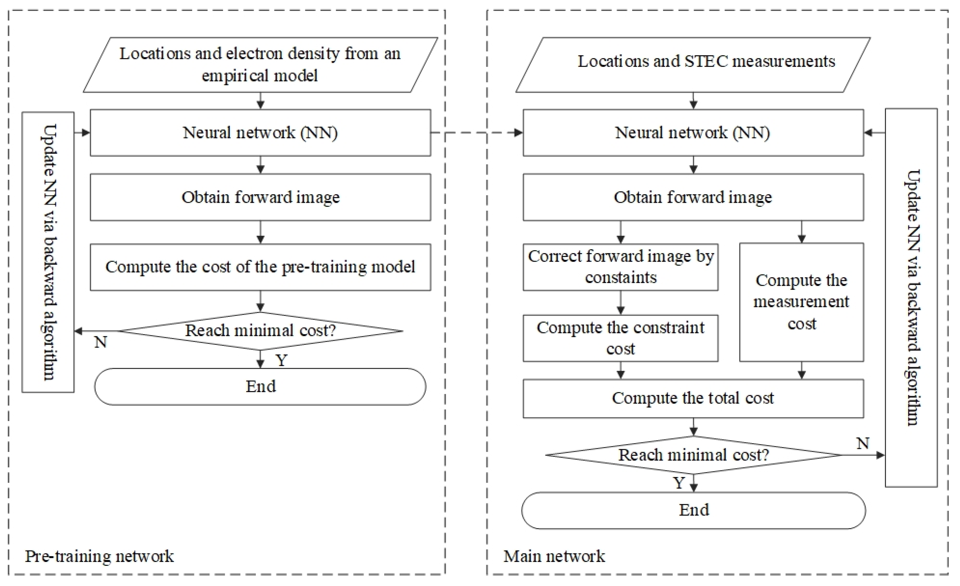
2.3. Pre-Training Process

The purpose of training in an NN is to obtain the parameters of the NN (i.e., weight and bias) for each neuro. In the training process, NN parameters are usually randomly initialized. Owing to the ill-posed problem of the ionospheric tomography, the choice of initial values would impact the obtained parameters, hence affecting the image quality. To get more reasonable initial values for the NN parameters, and to achieve a higher quality image, we pre-train the NN model by using an image extracted from an empirical ionosphere model, e.g., IRI-2016 [26]. Since every voxel is restrained by a value of electron density, the pre-training process is a well-posed problem. The cost function of the pre-training process is defined as

$$E=\sqrt{\frac{{{\displaystyle \sum }}_{j=1}^m{\left({\widehat{x}}_j-x_j^e\right)}^2}{m}}$$

(9)

where ${\widehat{x}}_j$ denotes the electron density of the jth voxel in the forward image, and $x_j^e$ indicates the electron density of the jth voxel from the empirical ionosphere model, and m is the total number of voxels.

3. Validations and Comparisons

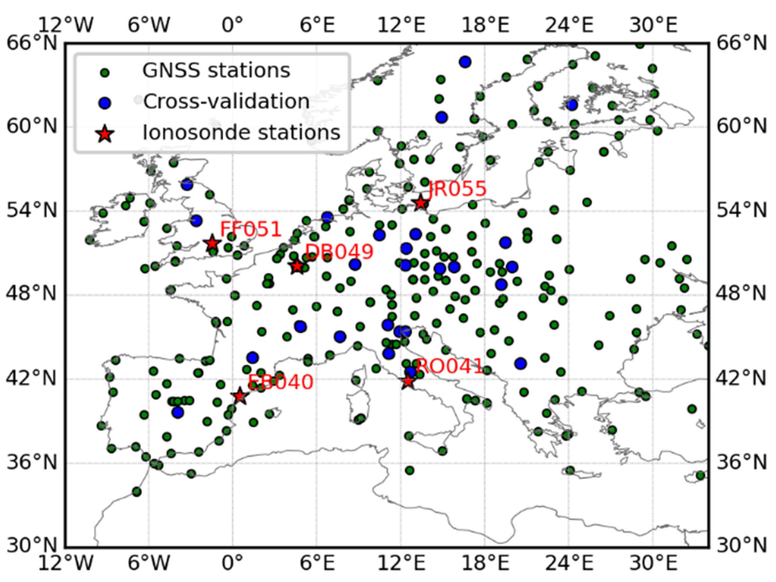
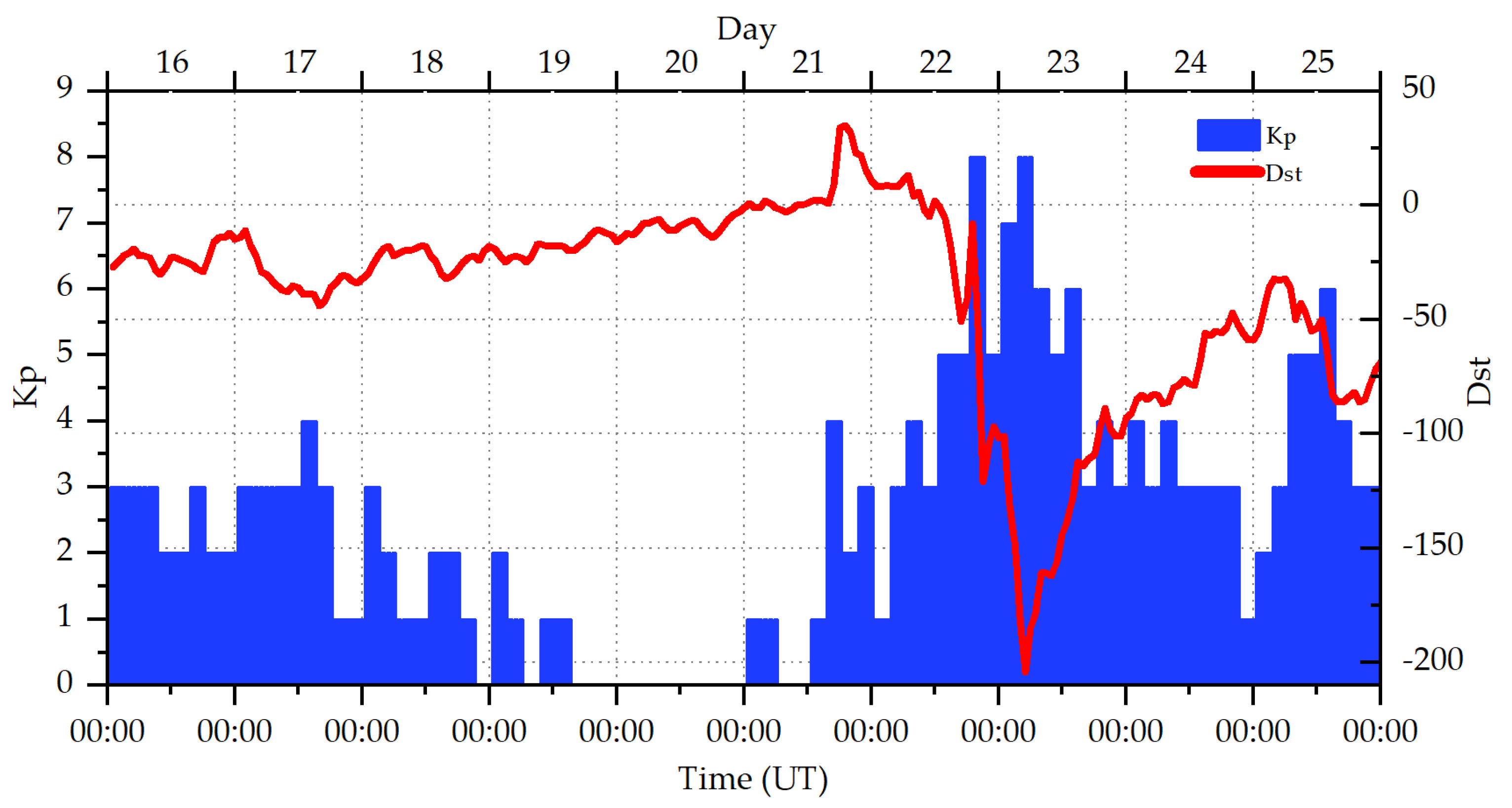
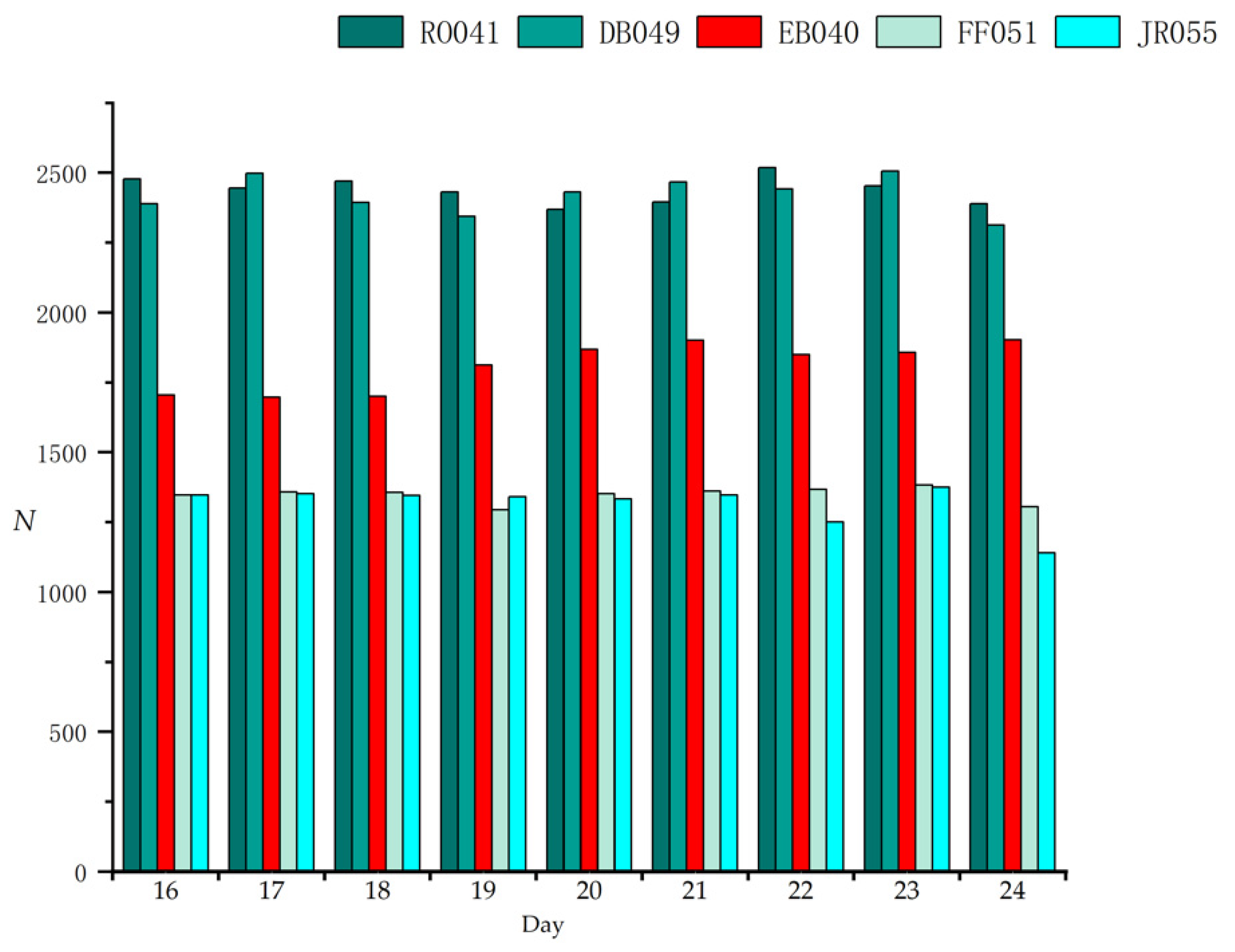
3.1. Data and Method

An area covering longitudes from 12° E to 34° E, latitudes from 30° N to 66° N, and heights from 100 km to 1200 km, and a span of ten days, from 16 June 2015 to 25 June 2015, were selected in this study. Figure 3 shows the study area and the distribution of GNSS stations. In this area, 226 GNSS stations and five ionosonde stations are available. We randomly chose 30 GNSS stations for cross-validation. Observations of vertical profile, peak density of F₂ layer (N_mF₂), peak height of F₂ layer (h_mF₂) obtained from the five ionosonde stations were used to validate the method. Furthermore, vertical total electron content (VTEC) map products from International GNSS service (IGS) center and the Technical University of Catalonia (UPC) were used in this validation. Figure 4 shows the Kp and Dst indices during the selected days. As shown, the ionosphere was experiencing an evident electromagnetic storm, where the Kp index is larger than 4 and the Dst index is smaller than or very close to −100, at midnight of 22 June and at noon on 25 June. Thus, a duration of four hours is selected for the nighttime (from 22:00 LT to 02:00 LT) and for the daytime (from LT 11:00 to LT 15:00), respectively, per day in this study.

The STEC measurements were obtained by a tool developed by Ionospheric Research Group (http://www.ionolab.org (accessed on 1 January 2022)) using a method given by Sezen et al. [32]. In the night, the plasmasphere has a significant contribution on the measured STEC. Following the way of Hong et al. [27], we considered the vertical TEC (VTEC) of the plasmasphere to be 3 TECU constantly during the whole day, and then removed it from the STEC measurement after mapping the VTEC onto a slant path, as shown by

$$s_{cor}=s_{obs}-\frac{v_{plas}}{\sin \alpha }$$

(10)

where $s_{cor}$ is the corrected STEC measurement, $\alpha$ is the elevation angle of the signal path, $v_{plas}$ is the VTEC of the plasmasphere, i.e., 3 TECU constantly.

We divided the ionosphere into 22,770 (23 × 18 × 55) voxels with a voxel size of 2° × 2° × 20 km and built an NN with four layers using a sigmoid activation function. The temporal resolution, the number of dominated EOFs and the balance parameter were set to be 15 min, 3 and 1, respectively. The NN parameters are iteratively updated by a back propagation algorithm [19]. The training process stops either at a minimal total cost or after 2000 times of iterations. To make a comparison, we selected the method developed by Farzaneh and Forootan [7] (named Slepian method hereafter), which selects spherical Slepian function and EOFs as the horizontal and vertical constraints, and the model of IRI-2016 [26] as references. Both the root mean square error (RMSE) and the improvement of the RMSE ($∆RMSE$) are calculated, as shown by

$$RMSE=\sqrt{\frac{{{\displaystyle \sum }}_{j=0}^m{({\widehat{x}}_j-x_j^T)}^2}{m}}$$

(11)

$$∆RMSE=\frac{\left(RMS{E}_r-RMS{E}_B\right)}{RMS{E}_r}\times 100\%$$

(12)

where $m$ refers to the number of samples, $\widehat{x}$ refers to the estimation, $x_j^T$ is the truth, $RMS{E}_r$ and $RMS{E}_B$ are the RMSE of the reference method and the BCDC model, respectively. Note that a positive value of the $RMS{E}_B$ shows an improvement of the BCDC model over the reference method.

3.2. Results

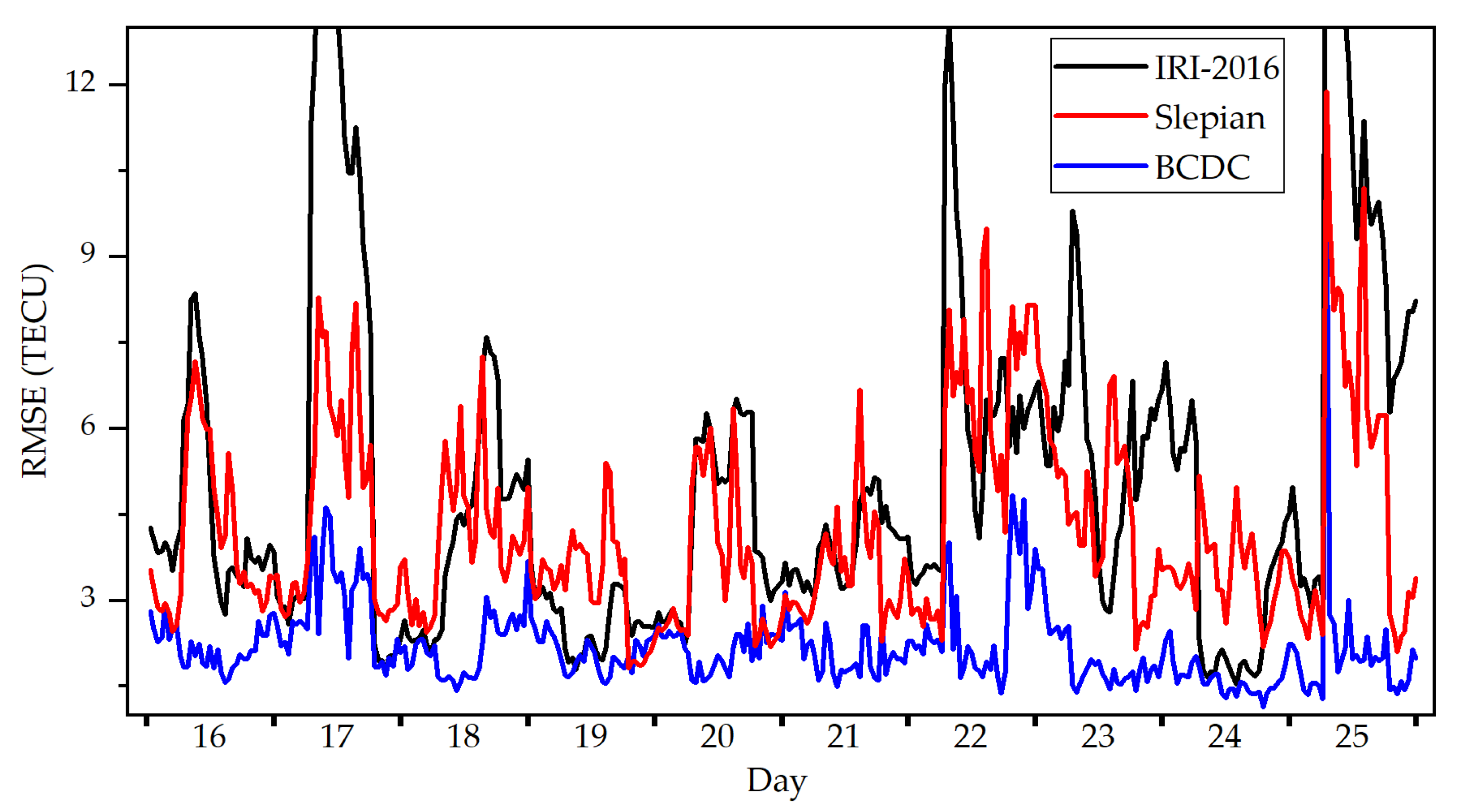
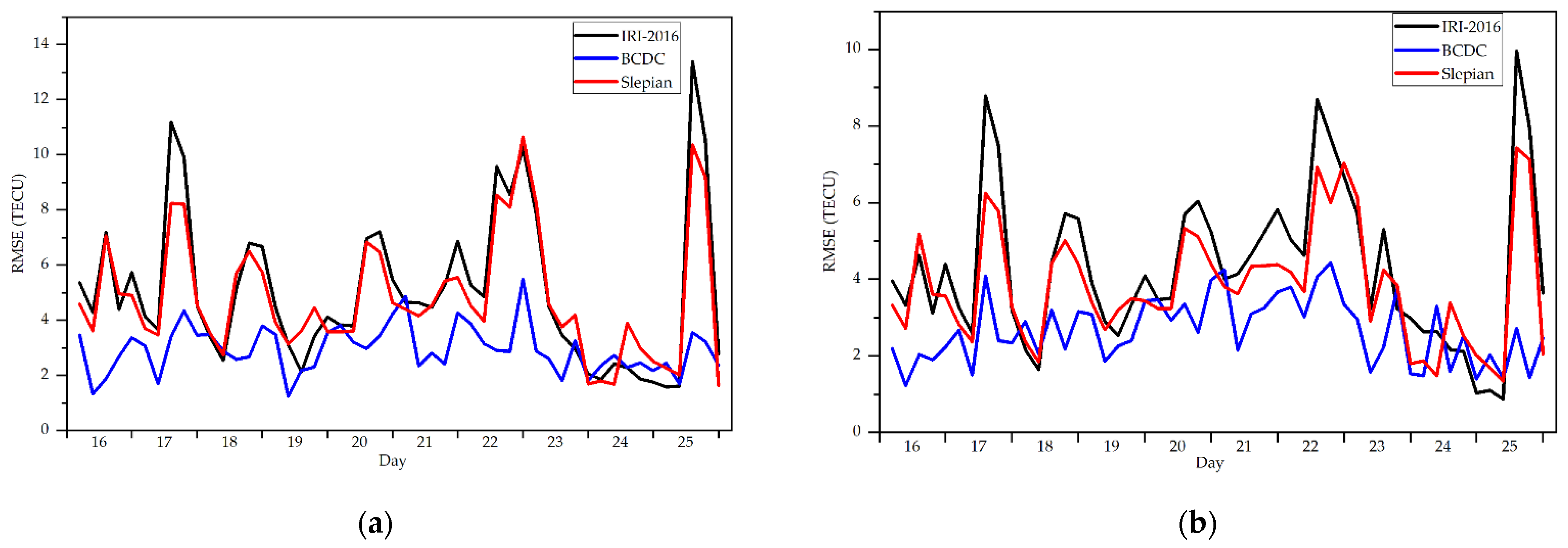
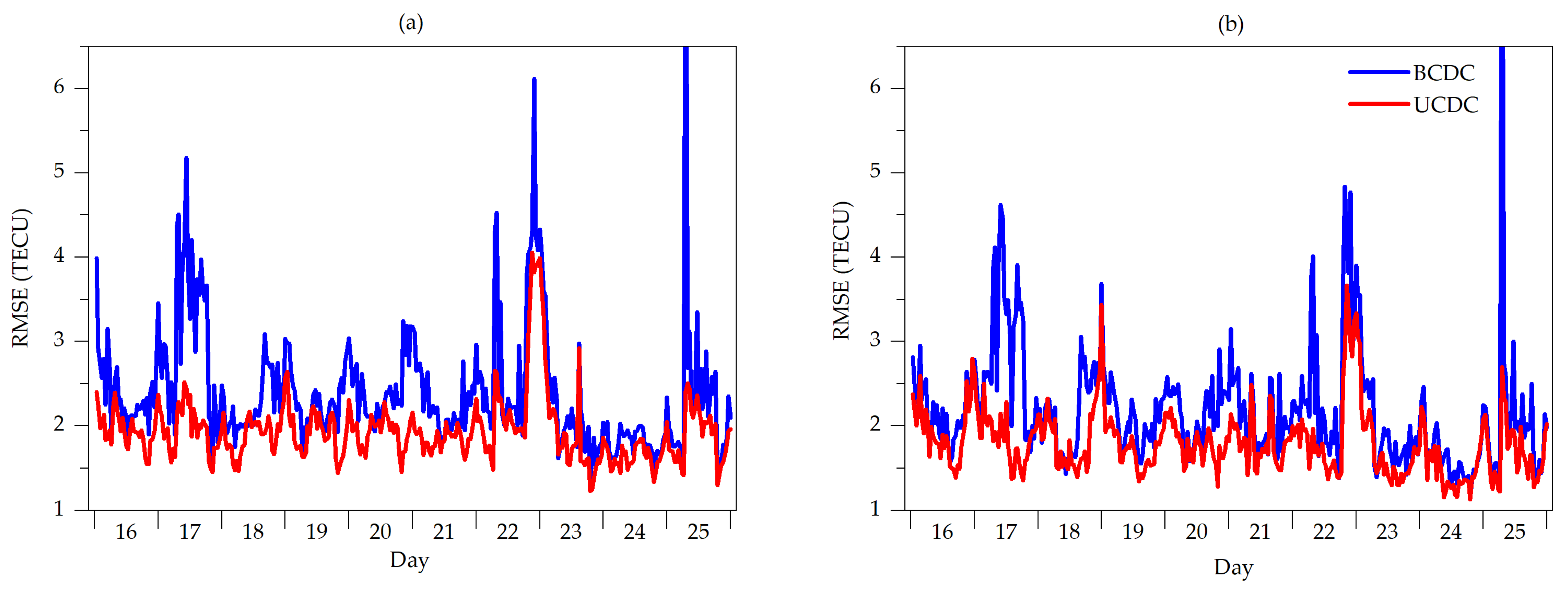
3.2.1. STEC Cross-Validations

Figure 5 shows the RMSE of the STEC derived by the BCDC method, the Slepian method and the IRI-2016 model at each moment. The BCDC method outperforms the other two at any time, and the Slepian method performs better than the IRI-2016 model most of the time.

Table 1. The RMSE (unit: TECU) and the ∆RMSE of the STEC derived by the BCDC, the IRI-2016, and the Slepian method for all moments.

	BCDC	Slepian	IRI-2016
RMSE	2.31	4.49	5.87
∆RMSE	-	48.6%	60.6%

compares the RMSE for all moments (called overall RMSE hereafter) among the three methods. The BCDC performs the best, followed by the Slepian method and the IRI-2016 model. The improvements of the overall RMSE achieved by the BCDC method over the Slepian method and the IRI-2016 model reach to 48.6% and 60.6%, respectively.

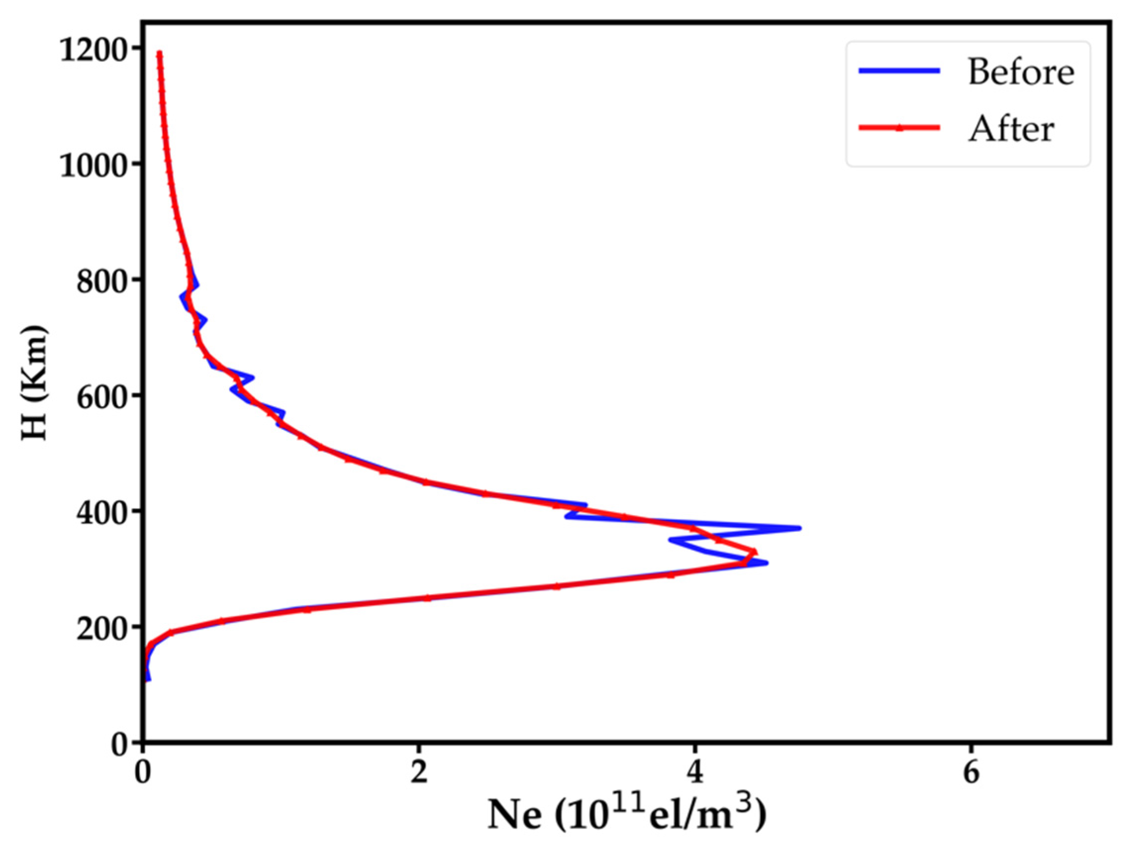
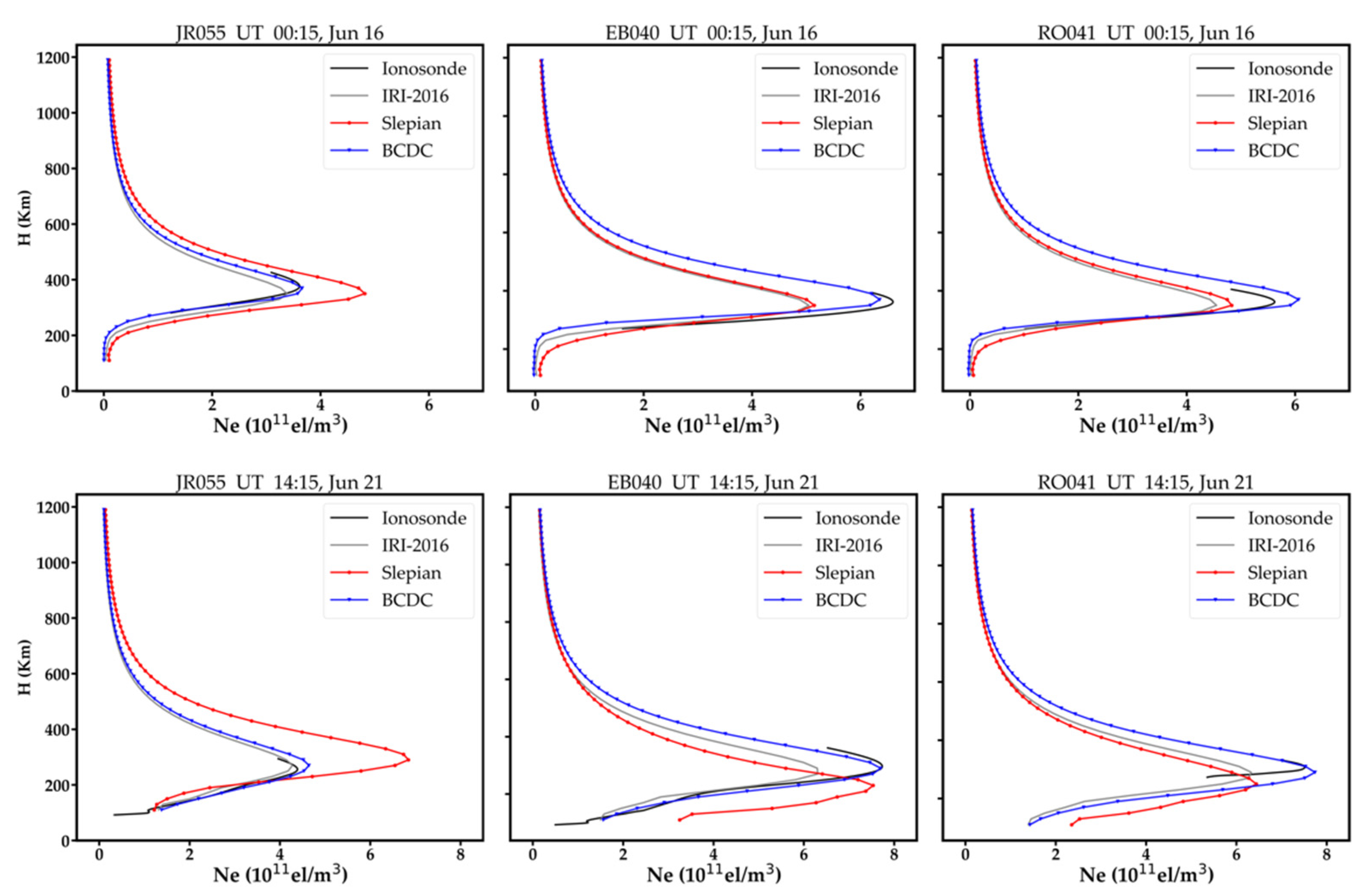
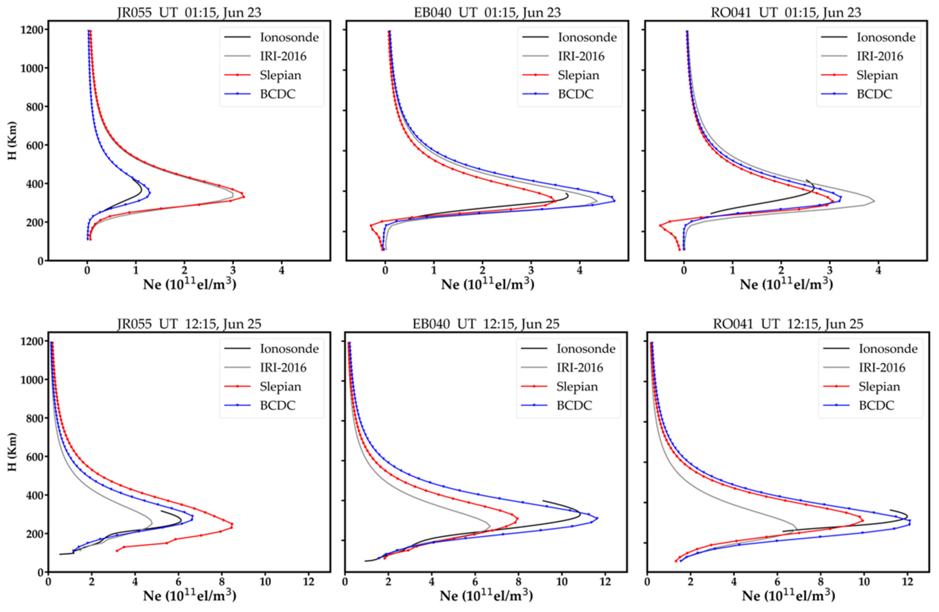
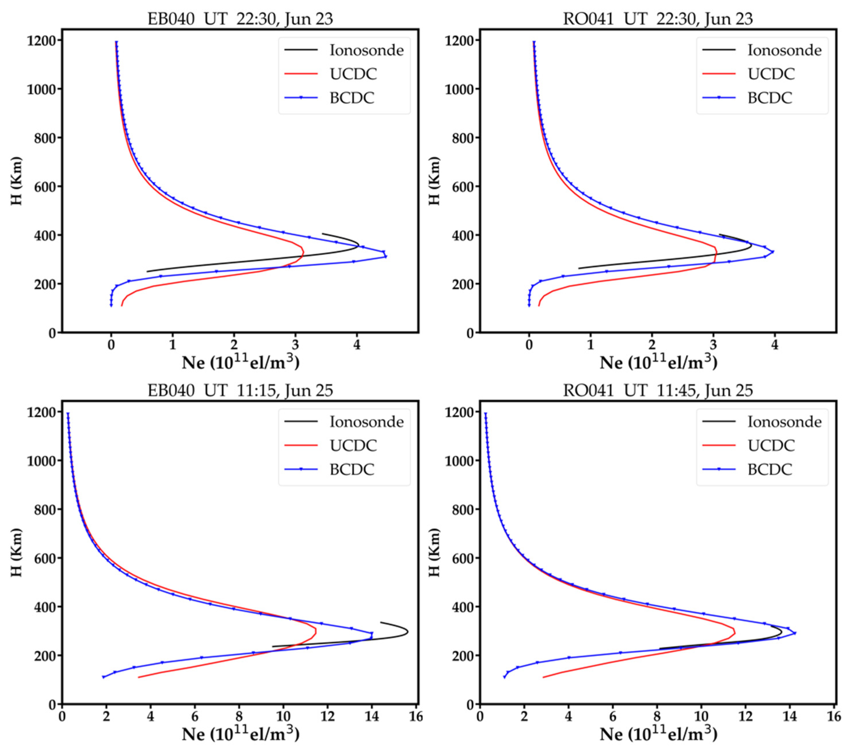
3.2.2. Vertical Profile Validations

There are five ionosonde stations in total in the study area. Figure 6 shows the number of signal paths that pass the voxels above these ionosonde stations on each day. As shown, the numbers of signal paths for the RO041 and DB049 are similar, and are larger than that of the EB040, which is larger than those of the FF051 and the JR055. For balance, we selected the vertical profiles obtained by the RO041, the EB040 and the JR055 to illustrate the comparison. Figure 7 and Figure 8 show a few samples of the vertical profiles derived from the three methods during the geomagnetic quiet time and geomagnetic disturbed time, respectively. Note that the topside profile above h_mF₂ are not measurements but estimations via Chapman or other similar functions fitting. Nearly all the vertical profiles of the BCDC method are closer to ionosonde than those of the Slepian method and the IRI-2016 model. Besides, negative values are observed on the vertical profiles of the Slepian, while those are disappeared in the BCDC method. This may be attributed to the adoption of the additional constraint of Chapman function in the BCDC method.

3.2.3. N_mF₂ and H_mF₂ Validations

The peak density of F₂ layer (N_mF₂) and peak height of F₂ layer (h_mF₂) are two important parameters in determining the vertical structure of the ionosphere.

Table 2. The overall RMSE (unit: 10¹¹ el/m³) and ∆RMSE of the N_mF₂ achieved by the three methods.

Stations	Methods	RMSE	∆RMSE	Stations	Methods	RMSE	∆RMSE
DB049	BCDC	0.82	-	JR055	BCDC	0.77	-
	IRI-2016	1.27	35.4%		IRI-2016	1.0	29.9%
	Slepian	0.93	9.7%		Slepian	1.29	40.3%
EB040	BCDC	1.10	-	FF051	BCDC	0.97	-
	IRI-2016	2.40	54.2%		IRI-2016	1.27	23.6%
	Slepian	1.98	44.4%		Slepian	1.05	7.6%
RO041	BCDC	1.11	-	Average	BCDC	0.95	-
	IRI-2016	2.24	50.4%		IRI-2016	1.64	42.1%
	Slepian	1.87	40.6%		Slepian	1.42	33.1%

presents the overall RMSE and the $∆RMSE$ of the N_mF₂ parameter per station. The BCDC outperforms the other two at all stations. The average improvements of the BCDC method over the Slepian method and the IRI-2016 model reach to 33.1% and 42.1%, respectively. Besides, the variation of the overall RMSE in the BCDC seems to be more stable than those in the Slepian and the IRI-2016.

Table 3. The overall RMSE and ∆RMSE of the H_mF₂ parameter (unit: km) achieved by the three methods.

Stations	Methods	RMSE	∆RMSE	Stations	Methods	RMSE	∆RMSE
DB049	BCDC	30.4	-	JR055	BCDC	26.6	-
	IRI-2016	28.1	−8.2%		IRI-2016	23.8	−11.8%
	Slepian	37.4	18.7%		Slepian	33.5	20.6%
EB040	BCDC	36.3	-	FF051	BCDC	37.6	-
	IRI-2016	33.7	−7.7%		IRI-2016	31.0	−21.3%
	Slepian	34.9	−4.0%		Slepian	35.5	−5.9%
RO041	BCDC	31.8	-	Average	BCDC	32.5	-
	IRI-2016	29.9	−6.4%		IRI-2016	29.3	−10.9%
	Slepian	32.0	0.6%		Slepian	34.7	6.3%

presents the overall RMSE and the $∆RMSE$ of the H_mF₂ parameter for the three methods. The BCDC method performs better than the Slepian method at DB049, JR055, RO041 stations but worse at the other stations, resulting in an average improvement of 6.3% over the Slepian method. However, both the BCDC method and the Slepian method perform worse than the IRI-2016 model. Nevertheless, their differences are less than 10 km, which is the half of the vertical size of a voxel in this study.

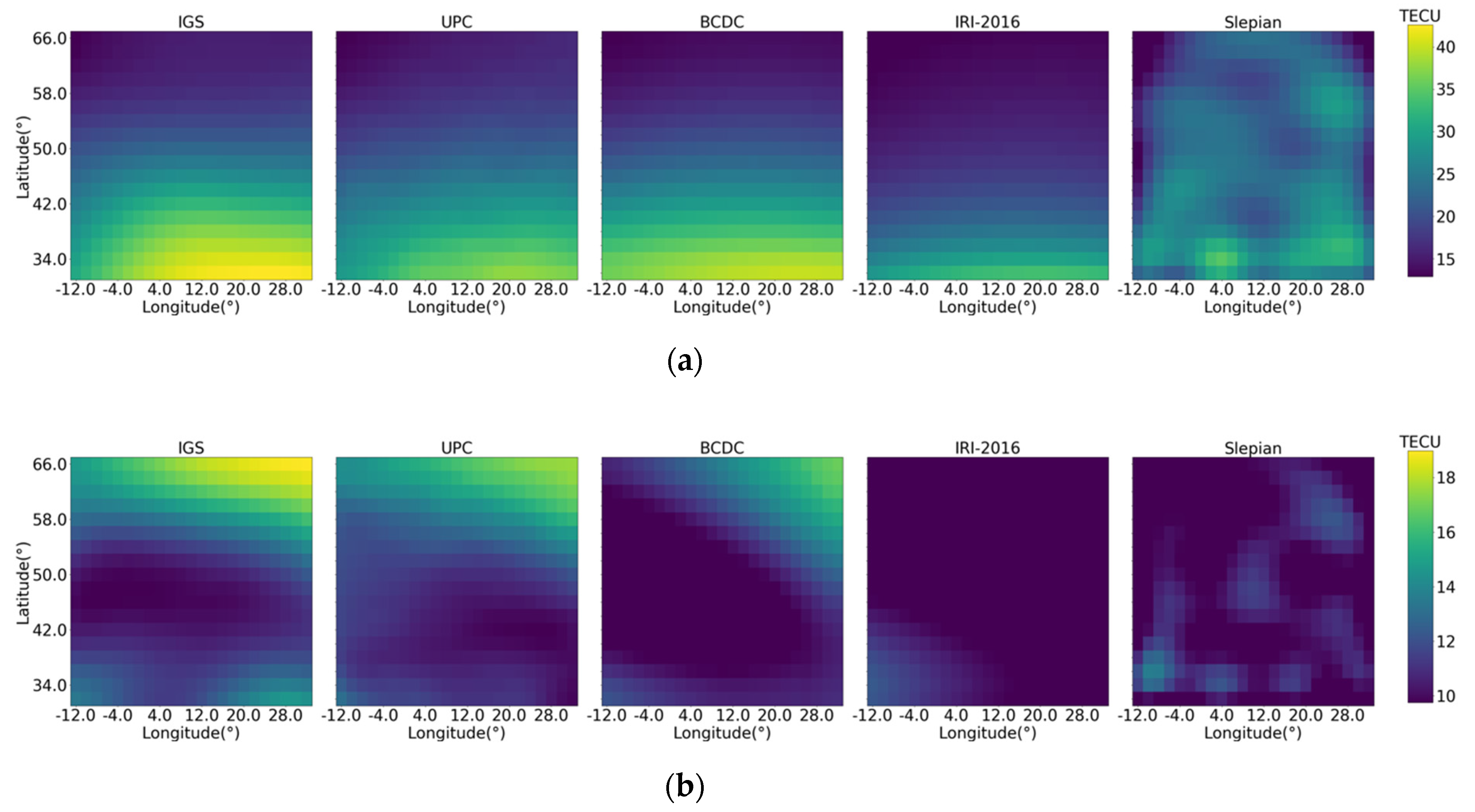
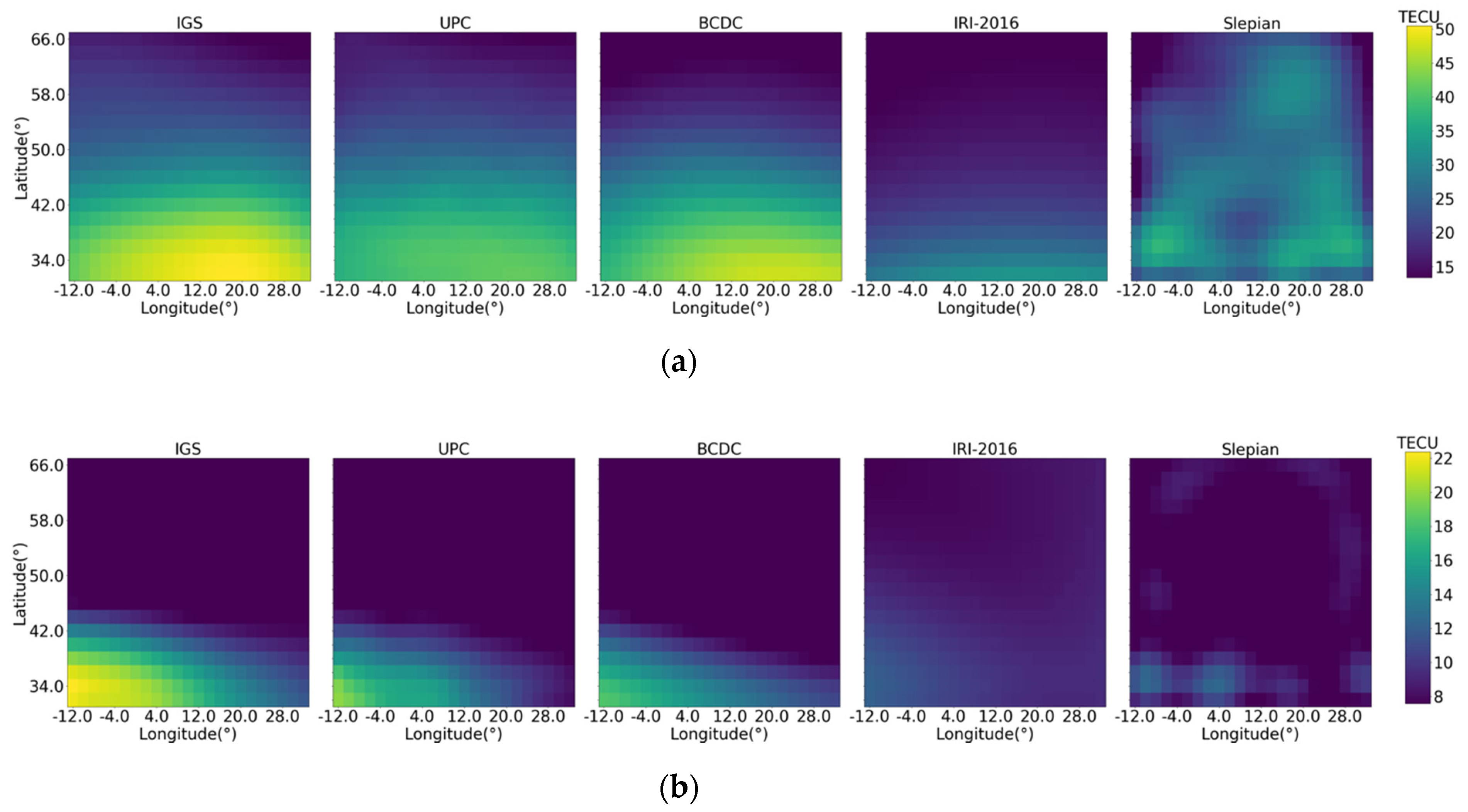
3.2.4. VTEC Validations

Figure 9 and Figure 10 shows the VTEC map produced by IGS, UPC, BCDC, IRI-2016 and Slepian during the geomagnetic quiet time and disturbed time, respectively. The VTEC maps produced by the BCDC are closer to those by IGS and UPC than those by the other two methods regardless of geomagnetic activity. Figure 11 compares the RMSE of the VTEC map produced by the BCDC, the Slepian and the IRI-2016 at each moment by taking that produced by IGS as the truth. The BCDC method performs better than the other two most of the time.

Table 4. The overall RMSE (unit: TECU) and the ∆RMSE of the VTEC derived by the BCDC, the IRI−2016, and the Slepian method with respect to UPC and IGS respectively.

	IGS			UPC
	BCDC	IRI-2016	Slepian	BCDC	IRI-2016	Slepian
RMSE	3.07	5.78	5.32	2.79	4.78	4.15
∆RMSE	-	46.9%	42.3%	-	41.6%	32.8%

lists the overall RMSE of the three methods by taking IGS and UPC as the truths. Obviously, the BCDC method outperforms the other two. The overall improvements of the BCDC method over the IRI-2016 model and the Slepian method reach to 46.9%, 42.3% with respect to IGS and 41.6%, 32.8% with respect to UPC.

4. Discussion

Balance cost function and the vertical constraint of EOFs are two main features of the BCDC method. This section discusses the benefit of the balance cost function and the choice of the number of the dominated EOFs.

4.1. Balance Cost Function

NN parameters are updated iteratively according to the model’s cost. Thus, how to define the cost function is crucial to an NN-based tomographic model. Usually, the cost function consists of a measurement cost and a constraint cost. In BCDC, the two costs are well balanced to avoid the produced image being inclined either to the measurements or to the constraints. To validate this, we compared the produced image with that by a model with the same flows and configurations as the BCDC but using an unbalanced cost function. For convenience, we refer the comparing model as unbalanced cost and dynamic correction neural network (UCDC). The cost function of the UCDC ($E^{\prime }$) is the same as it appears in most work, which is defined as

$$E^{\prime }=C_M+g\sqrt{\frac{{{\displaystyle \sum }}_{j=1}^m{\left({\widehat{x}}_j-x_j^c\right)}^2}{m}}$$

(13)

where $x_j^c$ refers to the electron density of the jth voxel after corrections, and the rests are the same as those in the above equations.

The constraint cost in UCDC is defined by the variable of election density. Note that STEC is the integral of the electron density along a signal path, which is longer the thickness of the ionosphere. Therefore, the value of STEC is always larger than the value of the electron density in several orders of magnitude. Under this circumstance, the measurement cost changes much faster than the constraint cost if the forward image is fluctuated. Since the goal of the training is to minimize the total cost, the image produced by the UCDC will be inclined to the STEC measurement. Figure 12 shows the RMSEs of the estimated STEC for each station used for tomography and used for cross-validation. Comparing with the BCDC, the RMSE of the estimated STEC by the UCDC is smaller, which agrees with the conclusion of the image being inclined to the STEC measurement in the UCDC method. However, smaller RMSE on the STEC parameter does not mean better quality.

Figure 13 shows the vertical profiles obtained by the two methods. Compared with the BCDC, the vertical profiles obtained by the UCDC around or below the F₂ layer seems to own a wider shape and show a larger discrepancy with the observed profiles. This is in accordance with the data shown in Figure 14. As the measurement cost dominates the training, the impact of the constraint become weak. A weaker vertical constraint gives more freedom to the model to adjust its vertical shape, making the vertical profiles distorted to better fit the STEC measurements. Though a smaller RMSE on the STEC parameter is observed in UCDC, its image is distorted and thus unreasonable. Therefore, an NN-based tomography model can benefit from a balance cost function.

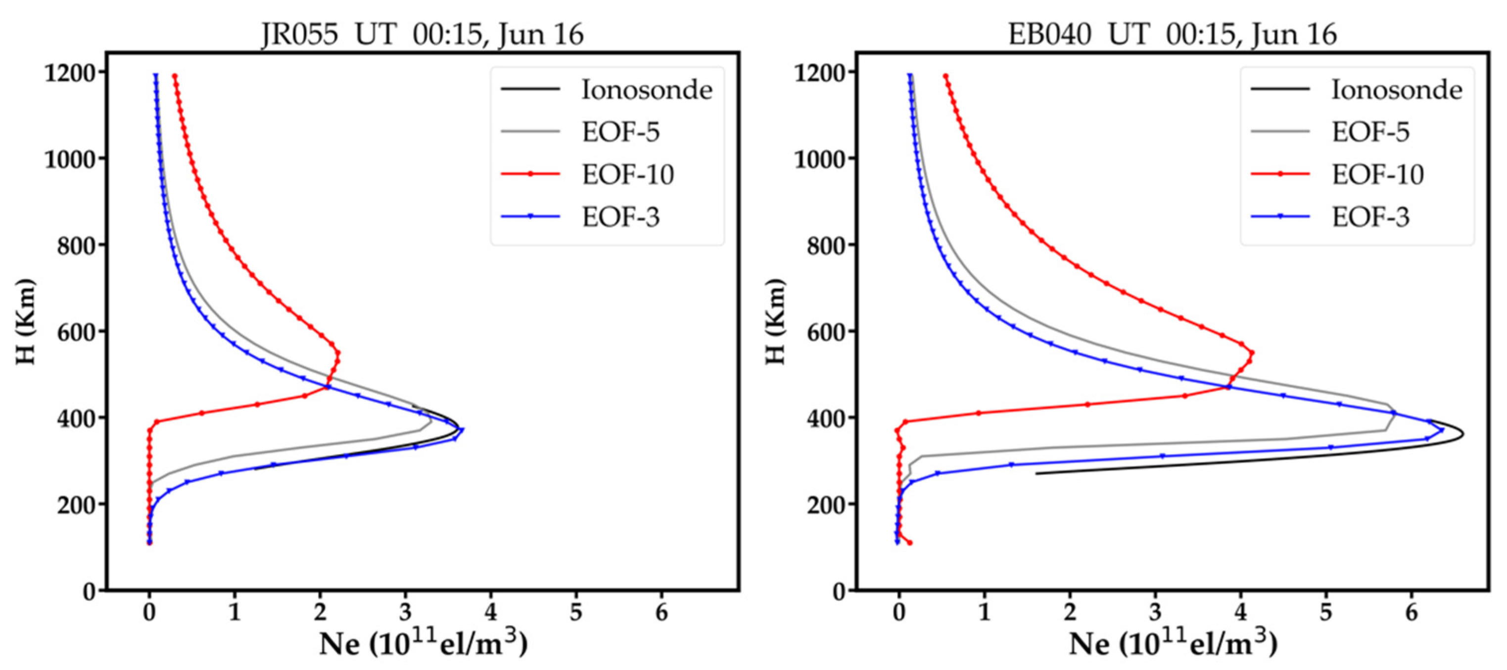
4.2. Number of Dominated EOFs

In the BCDC method, one of the corrections on the forward image is implemented by fitting each vertical profile with a few dominated EOFs. Decreasing the number of dominated EOFs give less freedom to the variation of the vertical profile, and vice versa. In other words, fewer dominated EOFs means a stronger constraint on the vertical profile, hence a smaller distortion is expected on the vertical profile. Figure 14 compares the vertical profiles that are obtained by three, five and ten dominated EOFs, respectively. Comparing to the ionosonde profiles, the vertical profiles achieved by ten EOFs show the largest distortion, followed by those achieved by five EOFs and three EOFs. Therefore, the number of the dominated EOFs in the BCDC method should not be very large.

5. Conclusions

A new tomographic model for ionospheric inversion based on neural network, named balance cost and dynamic correction (BCDC), is proposed. The BCDC model attempts to avoid the problem of undervaluing the selected constraints and the problem of the dependency on the preset images. The first problem is solved by using a cost function that well balances the measurement cost and the constraint cost. Tests show that an NN-based tomographic model can be benefited from a balance cost function. The second problem is solved by using a dynamically corrected image rather than a preset image. The forward image is corrected according to the constraints of EOFs, Chapman function and horizontal smoothing. Tests show that the number of the dominated EOFs should not be too large as the vertical constraint might become weak if too many EOFs are adopted.

A recently developed tomographic model, named Slepian in this paper, which also uses EOFs and horizontal smoothing as the constraints, as well as the IRI-2016 model, were selected as the references to compare with the BCDC method. Validations show that the BCDC method outperforms the other two in the comparisons of the STEC cross-validation, N_mF₂ parameters, vertical profiles and VTEC map. The BCDC method performs a bit better than the Slepian method, but both are worse than the IRI-2016 model in the comparison of the h_mF₂ parameter. Nevertheless, their differences are very small, which are less than the half size of a voxel vertically.

In BCDC, the network is simple, which may limit the capability of finding a more accurate solution for the model. Our future research will extend this to a deep neural network (DNN). Incorporating more measurements or more constraints into the model is will be considered in the near future.

References

1. Su, K.; Jin, S.; Hoque, M.M. Evaluation of Ionospheric Delay Effects on Multi-GNSS Positioning Performance. Remote Sens. 2019, 11, 171. [Google Scholar] [CrossRef] [Green Version]
2. Austen, J.R.; Franke, S.J.; Liu, C.H.; Yeh, K.C. Application of computerized tomography techniques to ionospheric research. In Proceedings of the International Beacon Satellite Symposium on Radio Beacon Contribution to the Study of Ionization and Dynamics of the Ionosphere and to Corrections to Geodesy and Technical Workshop, Oulu, Finland, 9–14 June 1986; pp. 25–35, Part 1. [Google Scholar]
3. Rius, A.; Ruffini, G.; Cucurull, L. Improving the vertical resolution of ionospheric tomography with GPS occultations. Geophys. Res. Lett. 1997, 24, 2291–2294. [Google Scholar] [CrossRef] [Green Version]
4. Raymund, T.D.; Austen, J.R.; Franke, S.J.; Liu, C.H.; Klobuchar, J.A.; Stalker, J. Application of computerized tomography to the investigation of ionospheric structures. Radio Sci. 1990, 25, 771–789. [Google Scholar] [CrossRef]
5. Pryse, S.E.; Kersley, L.; Rice, D.L.; Russell, C.D.; Walker, I.K. Tomographic imaging of the ionospheric mid-latitude trough. Ann. Geophys. 1993, 11, 144–149. [Google Scholar]
6. Bhuyan, K.; Singh, S.B.; Bhuyan, P.K. Tomographic reconstruction of the ionosphere using generalized singular value decomposition. Curr. Sci. India 2002, 83, 1117–1120. [Google Scholar]
7. Farzaneh, S.; Forootan, E. Reconstructing Regional Ionospheric Electron Density: A Combined Spherical Slepian Function and Empirical Orthogonal Function Approach. Surv. Geophys. 2018, 39, 289–309. [Google Scholar] [CrossRef] [Green Version]
8. Yao, Y.B.; Zhai, C.Z.; Kong, J.; Zhao, Q.; Zhao, C. A modified three-dimensional ionospheric tomography algorithm with side rays. GPS Solut. 2018, 22, 107. [Google Scholar] [CrossRef]
9. Chen, C.H.; Saito, A.; Lin, C.H.; Yamamoto, M.; Suzuki, S.; Seemala, G.K. Medium-scale traveling ionospheric disturbances by three-dimensional ionospheric GPS tomography. Earth Planets Space 2016, 68, 32. [Google Scholar] [CrossRef] [Green Version]
10. Chen, B.Y.; Wu, L.X.; Dai, W.J.; Luo, X.; Xu, Y. A new parameterized approach for ionospheric tomography. GPS Solut. 2019, 23, 96. [Google Scholar] [CrossRef] [Green Version]
11. Seemala, G.K.; Yamamoto, M.; Saito, A.; Chen, C.H. Three-dimensional GPS ionospheric tomography over Japan using constrained Least Squares. J. Geophys. Res. 2014, 119, 3044–3052. [Google Scholar] [CrossRef] [Green Version]
12. Zheng, D.Y.; Yao, Y.B.; Nie, W.F.; Liao, M.; Liang, J.; Ao, M. Ordered Subsets-Constrained ART Algorithm for Ionospheric Tomography by Combining VTEC Data. IEEE Trans. Geosci. Remote Sens. 2021, 59, 7051–7061. [Google Scholar] [CrossRef]
13. Wen, D.B.; Liu, S.J.; Tang, P.Y. Tomographic reconstruction of ionospheric electron density based on constrained algebraic reconstruction technique. GPS Solut. 2010, 14, 375–380. [Google Scholar] [CrossRef]
14. He, L.M.; Heki, K. Three-dimensional tomography of ionospheric anomalies immediately before the 2015 Illapel earthquake, Central Chile. J. Geophys. Res. Space 2018, 123, 4015–4025. [Google Scholar] [CrossRef] [Green Version]
15. Wen, D.B.; Yuan, Y.B.; Ou, J.K.; Zhang, K.; Liu, K. A hybrid reconstruction algorithm for 3-D ionospheric tomography. IEEE Trans. Geosci. Remote Sens. 2008, 46, 1733–1739. [Google Scholar] [CrossRef] [Green Version]
16. Zhao, H.S.; Yang, L.; Zhou, Y.L.; Ming, D. A AMART Algorithm Applied to Ionospheric Electron Reconstruction. Acta Geod. Cartogr. Sin. 2018, 47, 57–63. [Google Scholar] [CrossRef]
17. Gerzen, T.; Minkwitz, D. Simultaneous multiplicative column-normalized method (SMART) for 3-D ionosphere tomography in comparison to other algebraic methods. Ann. Geophys.-Ger. 2016, 34, 97–115. [Google Scholar] [CrossRef] [Green Version]
18. Ma, X.F.; Maruyama, T.; Ma, G.; Takeda, T. Three-dimensional ionospheric tomography using observation data of GPS ground receivers and ionosonde by neural network. J. Geophys. Res. Space 2005, 110, A05308. [Google Scholar] [CrossRef]
19. Rumelhart, D.E.; Hinton, G.E.; Williams, R.J. Learning internal representations by error propagation. In Parallel Distributed Processing; Rumelhart, D., Mclelland, J., Eds.; MIT Press: Cambridge, MA, USA, 1986; Volume 2, pp. 318–362. [Google Scholar]
20. Hirooka, S.; Hattori, K.; Takeda, T. Numerical validations of neural network based ionospheric tomography for disturbed ionospheric conditions and sparse data. Radio Sci. 2011, 46, 1–13. [Google Scholar] [CrossRef]
21. Razin, M.R.G.; Voosoghi, B. Regional application of multi-layer artificial neural networks in 3-D ionosphere tomography. Adv. Space Res. 2016, 58, 339–348. [Google Scholar] [CrossRef]
22. Razin, M.R.G.; Voosoghi, B. Ionosphere tomography using wavelet neural network and particle swarm optimization training algorithm in Iranian case study. GPS Solut. 2017, 21, 1301–1314. [Google Scholar] [CrossRef]
23. Zheng, D.Y.; Yao, Y.B.; Nie, W.F. A new three-dimensional computerized ionospheric tomography model based on a neural network. GPS Solut. 2020, 25, 10. [Google Scholar] [CrossRef]
24. Zheng, D.Y.; Yao, Y.B.; Nie, W.F.; Yang, W.; Hu, W.; Ao, M.; Zheng, H. An Improved Iterative Algorithm for Ionospheric Tomography Reconstruction by Using the Automatic Search Technology of Relaxation Factor. Radio Sci. 2018, 53, 1051–1066. [Google Scholar] [CrossRef]
25. Hannachi, A. Empirical Orthogonal Functions. In Patterns Identification and Data Mining in Weather and Climate; Springer Atmospheric Sciences; Springer: Cham, Switzerland, 2021; pp. 31–69. [Google Scholar] [CrossRef]
26. Bilitza, D.; Altadill, D.; Truhlik, V.; Shubin, V.; Galkin, I.; Reinisch, B.; Huang, X. International Reference Ionosphere 2016: From ionospheric climate to real-time weather predictions. Space Weather 2017, 15, 418–429. [Google Scholar] [CrossRef]
27. Hong, J.; Kim, Y.H.; Chung, J.K.; Ssessanga, N.; Kwak, Y.-S. Tomography reconstruction of ionospheric electron density with empirical orthonormal functions using Korea GNSS network. J. Astron. Space Sci. 2017, 34, 7–17. [Google Scholar] [CrossRef] [Green Version]
28. Dvinskikh, N.I. Expansion of ionospheric characteristics fields in empirical orthogonal functions. Adv. Space Res. 1988, 8, 179–187. [Google Scholar] [CrossRef]
29. Aa, E.; Ridley, A.; Huang, W.G.; Zou, S.; Liu, S.; Coster, A.J.; Zhang, S. An Ionosphere Specification Technique Based on Data Ingestion Algorithm and Empirical Orthogonal Function Analysis Method. Space Weather 2018, 16, 1410–1423. [Google Scholar] [CrossRef]
30. Chapman, S. The absorption and dissociative or ionizing effect of monochromatic radiation in an atmosphere on a rotating earth. Proc. Phys. Soc. 1931, 43, 26–45. [Google Scholar] [CrossRef]
31. Hernandez-Pajares, M.; Garcia-Fernandez, M.; Rius, A.; Notarpietro, R.; Von Engeln, A.; Olivares-Pulido, G.; Aragón-Àngel, À.; García-Rigo, A. Electron density extrapolation above F2 peak by the linear Vary-Chap model supporting new Global Navigation Satellite Systems-LEO occultation missions. J. Geophys. Res. Space 2017, 122, 9003–9014. [Google Scholar] [CrossRef]
32. Sezen, U.; Arikan, F.; Arikan, O.; Ugurlu, O.; Sadeghimorad, A. Online, automatic, near-real time estimation of GPS-TEC: IONOLAB-TEC. Space Weather 2013, 11, 297–305. [Google Scholar] [CrossRef]
Figure 1. Basic flows to implement the BCDC model.
Atmosphere 13 00426 g001
Figure 2. Comparison of the vertical profiles before and after the usage of the piecewise fitting and per-voxel averaging method.
Atmosphere 13 00426 g002
Figure 3. Study area and the distribution of GNSS stations and ionosonde stations.
Atmosphere 13 00426 g003
Figure 4. Kp and Dst indices during the experimental time on 16–25 June 2015.
Atmosphere 13 00426 g004
Figure 5. The RMSE (unit: TECU) of the STEC derived by the BCDC method, the Slepian method and the IRI−2016 model at each moment by taking the STEC measurements of the cross-validation stations as the truths.
Atmosphere 13 00426 g005
Figure 6. Number of signal paths (N) that pass the voxels above the ionosonde stations on each day.
Atmosphere 13 00426 g006
Figure 7. Vertical profiles obtained by the BCDC method, the Slepian method and the IRI−2016 model against those observed at JR055, EB040 and RO041 stations during the geomagnetic quiet time.
Atmosphere 13 00426 g007
Figure 8. Vertical profiles obtained by the BCDC method, the Slepian method and the IRI−2016 model against the those observed at JR055, EB040 and RO041 stations during the geomagnetic disturbed time.
Atmosphere 13 00426 g008
Figure 9. VTEC maps produced by IGS, UPC, BCDC, IRI−2016 and Slepian during the geomagnetic quiet time. (a) 12:00, 16 June; (b) 2:00, 21 June.
Atmosphere 13 00426 g009
Figure 10. VTEC maps produced by IGS, UPC, BCDC, IRI−2016 and Slepian during the geomagnetic disturbed time. (a) 12:00, 25 June; (b) 2:00, 23 June.
Atmosphere 13 00426 g010
Figure 11. The RMSE (unit: TECU) of the VTEC produced by the BCDC method, the Slepian method and the IRI−2016 model at each moment by taking the VTEC produced by IGS and UPC as truths. (a) IGS as the truth; (b) UPC as the truth.
Atmosphere 13 00426 g011
Figure 12. The RMSEs of the STEC parameter at each moment used for tomography (a) and cross-validation (b).
Atmosphere 13 00426 g012
Figure 13. Vertical profiles obtained by the BCDC and the UCDC at EB040 station (left column) and RO041 station (right column), respectively.
Atmosphere 13 00426 g013
Figure 14. Vertical profiles obtained by the BCDC model using three (EOF-3), five (EOF-5) and ten (EOF-10) EOFs at EB040 and JR055 at 00:15 LT on 25 June 2015.
Atmosphere 13 00426 g014