MCCS-LSTM: Extracting Full-Image Contextual Information and Multi-Scale Spatiotemporal Feature for Radar Echo Extrapolation

Abstract

Precipitation nowcasting has been gaining importance in the operational weather forecast, being essential for economic and social development. Conventional methods of precipitation nowcasting are mainly focused on the task of radar echo extrapolation. In recent years, deep learning methods have been used in this task. Nevertheless, raising the accuracy and extending the lead time of prediction remains as a challenging problem. To address the problem, we proposed a Multi-Scale Criss-Cross Attention Context Sensing Long Short-Term Memory (MCCS-LSTM). In this model, Context Sensing framework (CS framework) focuses on contextual correlations, and Multi-Scale Spatiotemporal block (MS block) with criss-cross attention is designed to extract multi-scale spatiotemporal feature and full-image dependency. To validate the effectiveness of our model, we conduct experiments on CIKM AnalytiCup 2017 data sets and Guangdong Province of China radar data sets. By comparing with existing deep learning models, the results demonstrate that the MCCS-LSTM has the best prediction performance, especially for predicting accuracy with longer lead times.

1. Introduction

The precipitation brought by strong convective weather has the characteristics of abruptness, intensity and unpredictability. Presently, precipitation nowcasting mainly refers to the prediction of rainfall intensity within a relatively short period (e.g., 0–6 h) in the future based on radar observation. The extrapolation of radar echo map has become one of the key methods for precipitation nowcasting [1]. One of the techniques for forecasting the evolution and the intensity of convective systems that has become especially interesting is the technique of radar echo extrapolation based on the historical sequences. Another one is based on the solution of a spatiotemporal sequences prediction problem. The process of radar extrapolation can be expressed by the following equation:

$$\widetilde{{\chi }_{t+1}}\dots ,\widetilde{{\chi }_{t+K}}=\underset{{\chi }_{t+1},\dots ,{\chi }_{t+K}}{argmax}p({\chi }_{t+1},\dots ,{\chi }_{t+K}\mid \widehat{{\chi }_{t-J+1}},\widehat{{\chi }_{t-J+2}},\dots ,\widehat{{\chi }_t})$$

(1)

where $\chi$ represents the observation tensor at any time, and $\widehat{{\chi }_{t-J+1}},\widehat{{\chi }_{t-J+2}},\dots ,\widehat{{\chi }_t}$ represent a sequence of tensors when we record the observations periodically. Through this equation, the task of radar echo extrapolation is to predict the most likely length-K sequence in the future based on the previous J observation sequences [2]. Once the extrapolated results is obtained, the precipitation distribution can be easily calculated with Z-R relationship [3]. Besides, accurate radar echo extrapolation result is the foundation of some forcasting algorithms [4,5], buliding an effective response to severe convective weather.

Radar echo sequences contain obvious spatiotemporal features. It is vital but difficult to overcome the uncertainty between adjacent frames, which makes the radar echo extrapolation problem challenging. Besides, there is a nonlinear relationship between meteorological factors. Traditional methods are not good at modeling the spatiotemporal relationships. To address this problem, more and more researchers try to adopt neural networks to deal with this complex relationship. Recently, radar echo extrapolation technology based on deep learning [6] has made significant progress. Many researchers have proposed a series of models based on convolutional neural network and recurrent neural network to extract the spatiotemporal characteristics of radar echo sequences. To take the spatiotemporal correlations of radar echo into consideration, Shi et al. proposed Convolutional Long Short-Term Memory (ConvLSTM) [2] by stacking several ConvLSTM layers to build an end-to-end model, andfurthermore the precipitation nowcasting is modeled as the spatiotemporal sequences prediction problem. Wang et al. proposed a novel convolutional LSTM unit to build a Predictive RNN (PredRNN) [7] network for radar extrapolations. Wang et al. further improved the PredRNN network and thus proposed PredRNN++ [8] by introducing a Casual LSTM unit and a gradient Highway Unit. Specifically, the application of the spatiotemporal long short-term memory(LSTM) and the Casual LSTM enable models to capture spatiotemporal correlation better. Wu et al. used a combination of 3D Convolutional Neural Networks (3DCNN) and LSTM [9] to predict the precipitation in a specific area, and achieved stable operation on the weather station platform. Wang et al. developed a predictive network that can capture non-stationary and approximately stationary properties in radar echo extrapolation, and proposed the Memory In Memory (MIM) network [10]. Luo et al. proposed an LSTM model with Interaction Dual Attention (IDA-LSTM) [11] which can solve the problem of underestimating the high echo value areas is solved by developing an interaction framework and dual attention for ConvRNN unit.

Nevertheless, most of the previously given techniques only focus on the global spatiotemporal flows of given frames in the hidden states, ignoring the multi-scale variations between adjacent frames and the correlation between the current input and upper context. Especially, in the task of radar echo extrapolation, the current input and upper context refer to the radar echo image of the current time and the last time, respectively. As the prediction time increases, the radar echo predicted image gradually becomes blurred and the radar echo region with higher reflectivity has the tendency to disappear, which impact the accuracy.

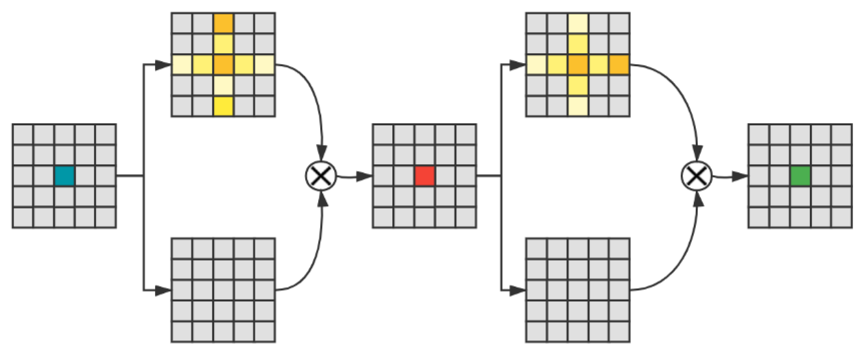
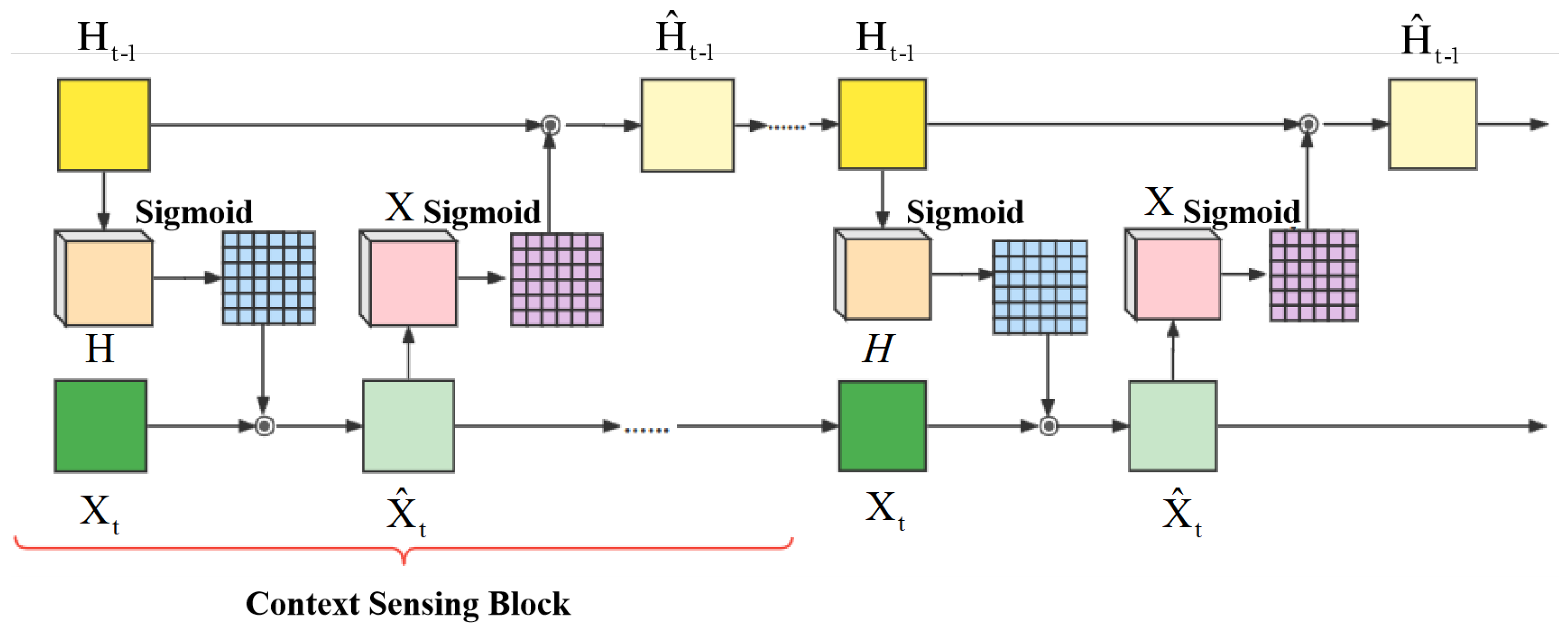
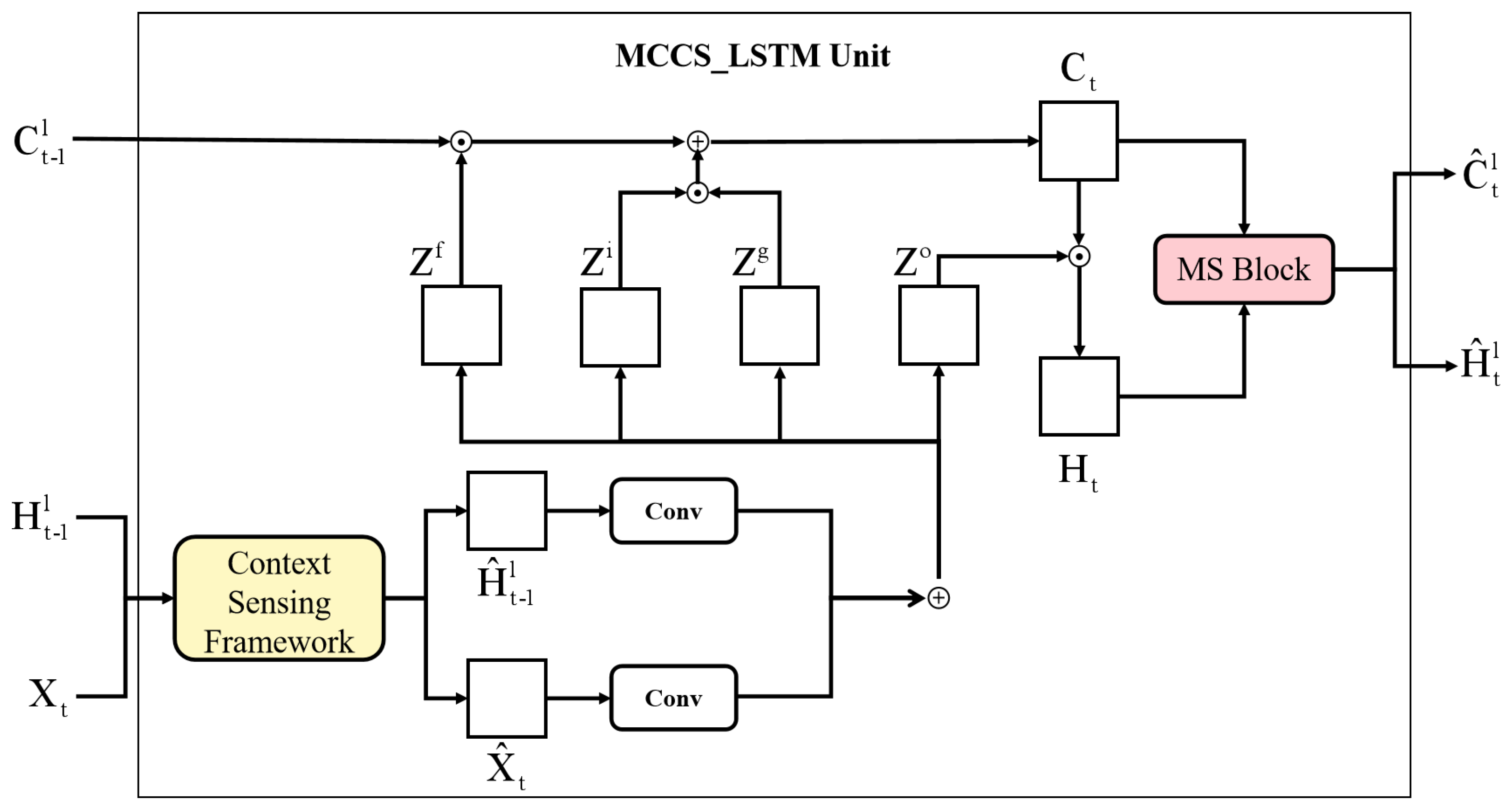
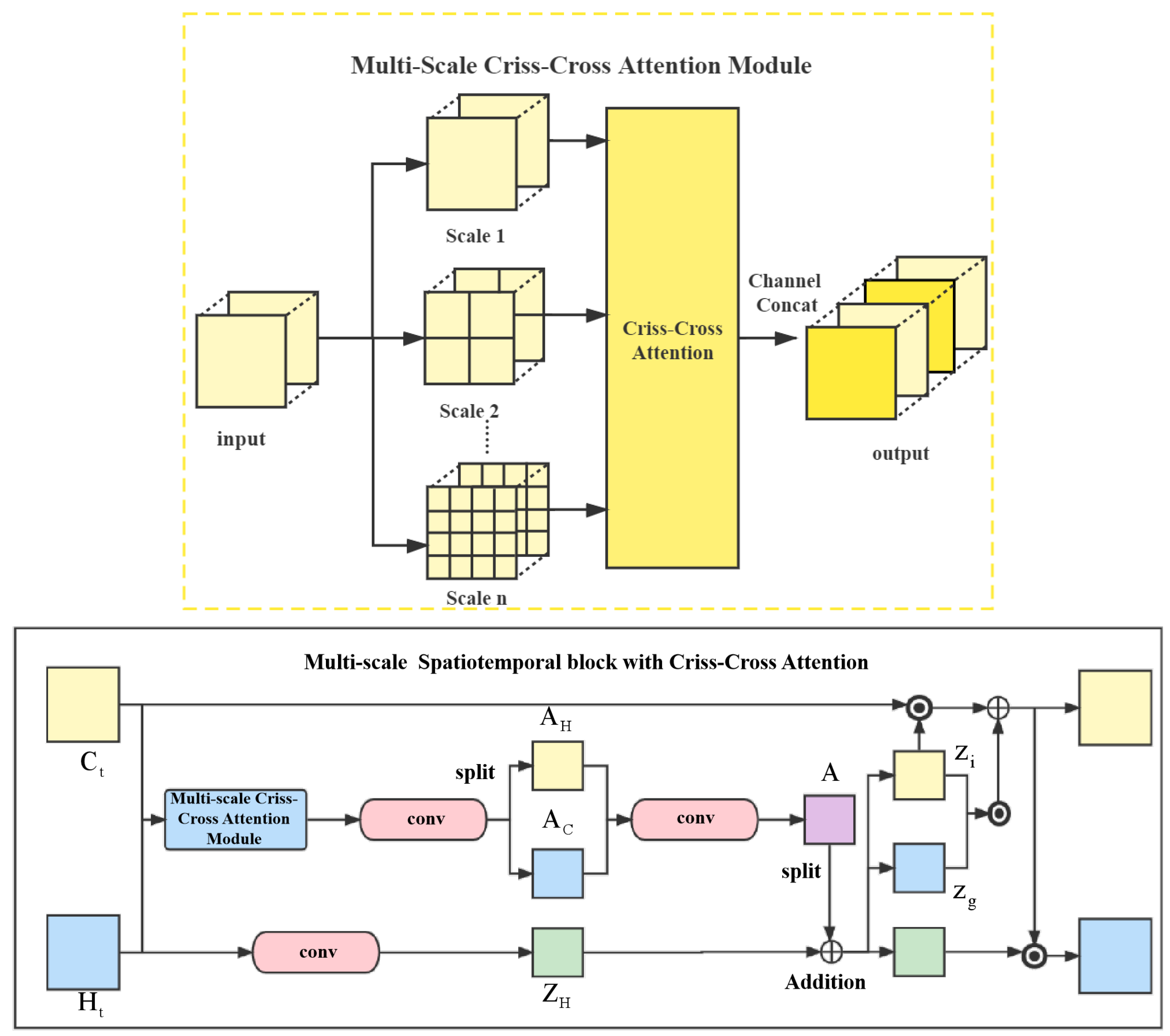
In order to overcome the limitations of previous works, in this paper, we propose Muti-Scale Criss-Cross Attention Context Sensing Long Short-term Memory (MCCS-LSTM), as an extension structure of ConvLSTM. Specifically, (1) Multi-Scale Spatiotemporal block with criss-cross attention (MS block) is designed to capture full-image dependencies and abundant spatiotemporal flows in different scales between sequences, building the short-term dependency adaptively. (2) Context Sensing block (CS block) is designed to capture the input and context correlations, maintaining the spatiotemporal consistency among long sequences and building the long-term dependency adaptively. In summary, our main contributions are as follows:

• We introduce two model structures, namely Multi-Scale Spatiotemporal block with criss-cross attention (MS block) and Context Sensing framework (CS framework). MS block can extract multi-scale spatiotemporal feature and develop full-image dependency. CS Framework can capture correlations between the current input and upper context.
• Our MCCS-LSTM innovatively adopts a criss-cross attention mechanism and context-sensing structure, and experimental results show MCCS-LSTM is superior to previous model.

2. Related Work

2.1. ConvLSTM

In the past few years, recurrent neural network and LSTM have been widely used in spatiotemporal sequence forecasting problem. Among them, the improved model based on convolutional LSTM is one of the important branches. PredRNN and PredRNN++ achieved better prediction effects by introducing spatiotemporal memory units. MIM updated memory units in LSTM into spatiotemporal expression calculation of non-stationary and stationary information. IDA-LSTM combine ConvLSTM with dual attention to recall the forgotten information. In conclusion, spatiotemporal feature extraction through the combination of LSTM and convolutional neural network is an effective solution for radar echo extrapolation. Therefore, the new model proposed in this paper is improved on the basis of convolutional LSTM structure.

Unlike the LSTM model structure used for one-dimensional time series data, this model combines convolution with LSTM so that this structure can capture spatial and temporal features. The structure of ConvLSTM is shown in Figure 1, where the three gate structures of ConvLSTM are forget gate $f_t$, input gate $i_t$ and output gate $o_t$. $C_t$ is a memory cell. The memory cell does not only retains the current input characteristics, but also controls whether the information at the previous moment continues to be transmitted. The information transmission relationship is expressed by equation:

$$\begin{array}{c}{i}_t=\sigma (W_{xi}\ast X_t+W_{hi}\ast H_{t-1}+W_{ci}\ast C_{t-1}+b_i)\hfill \\ f_t=\sigma (W_{xf}\ast X_t+W_{hf}\ast H_{t-1}+W_{cf}\ast C_{t-1}+b_f)\hfill \\ C_t=f_t\circ C_{t-1}+i_t\circ tanh(W_{xc}\ast X_t+W_{hc}\ast H_{t-1}+b_c)\hfill \\ o_t=\sigma (W_{xo}\ast X_t+W_{ho}\ast H_{t-1}+W_{co}\circ H_{t-1}+b_o)\hfill \\ H_t=o_t\circ tanh\left(C_t\right)\hfill \end{array}$$

(2)

where $\sigma$, ∘, ∗ denotes sigmoid activation function, matrix multiplication, convolution operation, respectively. $X_t$ is the input, $C_t$ is the memory cell, $H_t$ is the hidden state, $i_t$ is the input gate, $f_t$ is the forget gate, and $o_t$ is the output gate. Specifically, the convolution operation is used to extract the features, and the information is selected through the gate structure. The forget gate controls which information will be forgotten in the previous state $X_t$ and $H_{t-1}$, and then the information flows into the input gate which determines which information will be updated through sigmoid function, and the update operation will be done through tanh activation function. The final ouput $H_t$ will be obtained from the multiplication product of the information from the output gate and the information flows from that layer [2].

2.2. Contextual Information Aggregation

In the spatiotemporal sequence forecasting problem, the previous models ignore the relationship between the current input and the context, which are independent of each other. With the increase of model’s complexity, the correlation between the current input and the context will decrease with the information flows among layers.

In semantic segmentation, for purpose of augmenting the feature representation, the current models normally adopt the method of aggregating contextual information. Deeplabv2 [12] proposed Atrous Spatial Pyramid Pooling (ASPP), which can capture context information through different expansion convolution. Chen et al. [13] applied the attention mechanism to fuse different feature maps and aggregate contextual information. Huang et al. [14] proposed a new attention mechanism called criss-cross attention to capture full-image contextual information. The criss-cross attention is demonstrated in Figure 2.

From this module, the contextual information is added to feature map, obtaining a wide contextual view. Therefore, it can aggregates contexts and enhance feature representations. Therefore this new attention mechanism is used in our new model to settle the issue of radar echo extrapolation.

3. Methods

In this section, we will present the MCCS-LSTM model in detail. Firstly, the context sensing framework is given, and then we elaborate multi-scale spatiotemporal block with criss-cross attention and portray how to embed CS framework and MS block into our model. Finally, we will present the whole structure of the proposed MCCS-LSTM model.

3.1. Context Sensing Framework

In previous LSTM based models such as PredRNN, the current input $X_t$ and the previous hidden state $H_{t-1}$ independently enter into LSTM layers. Therefore, with the increasing depth of the model, correlations between the current input and upper context tend to disappear. In fact, there is a certain correlation between the current input and upper context. In pursuit of extracting this correlation, we introduce context sensing framework with the inspiration of the previous work [15]. As shown in Figure 3, we exploit this framework to extract abundant correlational information.

Equations of the context sensing framework can be presented as follows:

$$\begin{array}{c}\widehat{X_t}=\sigma (W_H\ast H_{t-1}+b_H)\circ X_t\hfill \\ \widehat{H_{t-1}}=\sigma (W_X\ast \widehat{X_t}+b_X)\circ H_{t-1}\hfill \end{array}$$

(3)

where $X_t$ denotes current input, $H_{t-1}$ denotes the previous state, $\sigma$ is the element-wise sigmoid function, ∘ stands for matrix product. $X_t$ and $H_{t-1}$ are fed into context sensing framework, and then $\widehat{X_t}$ and $\widehat{H_{t-1}}$ can be obtained through several context sensing blocks. In our model, we set the number of context sensing block as four. Specifically, $H_{t-1}$ is fed into 5 × 5 convolution layers and multiply with $X_t$ to obtain the $\widehat{X_t}$ Similarly, after 5 × 5 convolution operation, $\widehat{X_t}$ multipy with $H_{t-1}$ to obtain $\widehat{H_{t-1}}$. Finally, $\widehat{X_t}$ and $\widehat{H_{t-1}}$ represent current input and the previous state after context sensing framework, respectively.

3.2. Multi-Scale Spatiotemporal Block with Criss-Cross Attention

During the evolution of radar echo, when sudden changes occur, pixel-level changes between adjacent frames occasionally happen in specific regions. So it is essential to model video dynamics in different spatiotemporal scales. Inspired by previous work [16,17], we proposed MS block to extract more implicit features in spatiotemporal flows.

The self-attention mechanism can extract important parts of feature maps. In order to model full-image dependencies over local feature, we use criss-cross attention as shown in Section 2.2 of the article. Besides, $C_t$ and $H_t$ contain spatiotemporal flows, while in the process of feature extraction in adjacent sequences, more potential tendencies can be captured by using multi-scale regions. Namely, MS block can extract multi-scale spatiotemporal flows. As shown in Figure 4, $H_t$, $C_t$∈${\mathbb{R}}^{C\times H\times W}$ are stacked into Z∈${\mathbb{R}}^{C\times H\times W\times 2}$. Then Z is divided into n multi-scale groups $Z_1$, $Z_2$, …, $Z_n$, and each $Z_i$ is stacked in C to compose $\widehat{Z_1}$, $\widehat{Z_2}$, …, $\widehat{Z_n}$. Each $\widehat{Z_i}$ is fed into Criss-Cross Attention module, and, respectively, obtain $\widehat{z_1}$, $\widehat{z_2}$, …, $\widehat{z_n}$. Finally, $\widehat{z_1}$, $\widehat{z_2}$, …, $\widehat{z_n}$ are stacked to the output z∈${\mathbb{R}}^{nC\times H\times W\times 2}$. In this paper n is set to 3, namely the input is divided into 3 multi-scale groups. The spatiotemporal states $H_t$, $C_t$ are stacked and then fed into Multi-Scale Criss-Cross Attention Module to obtain z. Then we take z as input, and 5 × 5 convolution layer is applied to generate feature maps $A_H$ and $A_C$. $A_H$ and $A_C$ are stacked in C channel as the input of 5 × 5 convolution layer to obtain a multi-scale attention map A. Meanwhile, $Z_H$ is generated from hidden state C after going through a 5 × 5 convolution layer. Add A to $Z_H$ and split the result into 3 parts: $z^i$, $z^g$ and $z^o$. Formally, $C_t$ and $H_t$ are updated as follows:

$$\begin{array}{c}{z}^i=\sigma (W_{A_i}\ast [A_H,A_C]+W_{h_i}\ast Z_H+b_i)\hfill \\ z^g=tanh(W_{A_g}\ast [A_H,A_C]+W_{h_g}\ast Z_H+b_g)\hfill \\ z^o=tanh(W_{A_o}\ast [A_H,A_C]+W_{h_o}\ast Z_H+b_o)\hfill \\ \widehat{C_t}=(1-z^i)\circ C_t+z^i\circ z^g\hfill \\ \widehat{H_t}=z^o\circ C_t\hfill \end{array}$$

(4)

where $[A_H,A_C]$ represents the stacking result of $A_H$ and $A_C$. After this update, the output state and memory of LSTM can extract multi-scale spatiotemporal flows and contextual information.

3.3. MCCS-LSTM

In order to take into account of contextual information and multi-scale implicit features, we proposed MCCS-LSTM by applying CS framework and MS block into LSTM. Figure 5 illustrates the inside structure of MCCS-LSTM unit, where $H_{t-1}$ denotes the output state of $t-1$ time, $C_{t-1}$ represents memory state of $t-1$ time, $X_t$ denotes the input of t time, $\widehat{H_t}$ represents the output through MCCS-LSTM unit of t, and $\widehat{C_t}$ represents memory state of t. Formally, the calculation of MCCS-LSTM unit can be expressed as follows:

$$\begin{array}{c}\widehat{X_t},\widehat{H_{t-1}}=CS(X_t,H_{t-1})\hfill \\ i_t=\sigma (W_{xi}\ast \widehat{X_t}+W_{hi}\ast \widehat{H_{t-1}}+b_i)\hfill \\ g_t=tanh(W_{xg}\ast \widehat{X_t}+W_{ht}\ast \widehat{H_{t-1}}+b_g)\hfill \\ f_t=\sigma (W_{xf}\ast \widehat{X_t}+W_{hf}\ast \widehat{H_{t-1}}+b_f)\hfill \\ C_t=f_t\circ C_{t-1}+i_t\circ g_t\hfill \\ o_t=\sigma (W_{xo}\ast \widehat{X_t}+W_{ho}\ast \widehat{H_{t-1}}+b_o)\hfill \\ H_t=o_t\circ tanh\left(C_t\right)\hfill \\ \widehat{H_t},\widehat{C_t}=MS(H_t,C_t)\hfill \end{array}$$

(5)

where ∘ denotes the Hadamard product, ∗ denotes the 2D convolution. Obviously, both contextual information and multi-scale implicit features are extracted by this unit.

The architecture of MCCS-LSTM model is shown in Figure 6. We stack four MCCS-LSTM units to build a network. In this network, we update the spatial memory cells in a zigzag direction, and update temporal memory information in the horizontal direction. The top layer outputs the prediction result $\widehat{X_t}$. Therefore, the whole MCCS-LSTM model extracts highly abstract features by stacking MCCS-LSTM units to obtain great spatiotemporal modeling capability. In this paper, we stack four MCCS-LSTM units.

4. Experiment

In this section, we evaluate the proposed MCCS-LSTM model and compare with some state-of-the-art models.

4.1. Experiment Details

In this part, we will present the implementation details including the dataset, parameters, evaluation metrics, and training setting.

4.1.1. Dataset

We conducted experiments on two diffient data sets to verify the strong applicability and generalization of our model. The first radar echo dataset is from the Conference on Information and Knowledge Management (CIKM) AnalytiCup 2017 competition. This radar echo maps dataset covers 101 × 101 km area in Shenzhen City and the size of each map is 101 × 101 (pixel). In order to facilitate the calculation of deep learning, we resize the image size to 104 × 104 (pixel) with the operation of padding. Besides, the original dataset contains a training set with 10,000 samples and a testing set with 4000 samples, and each sample includes 15 radar echo maps with an interval of six minutes. We take the first five consecutive radar echo maps as input and predict the last ten. Namely, we predict radar echo maps for the next 60 min based on observations from the past 30 min. A total of 2000 samples were randomly selected from training set as the validation set.

The second radar echo dataset used in this paper consists of three-year radar intensities collected in Guangdong Province of China from 2018 to 2020. We extract Constant Altitude Plan Position Indicator (CAPPI) images from original data. Our experimental radar maps are resized to 100 × 100 by using down-sampling. The resolution of radar map is changed to ${0.1}^{\circ }$ (10 km × 10 km) in order to be more suitable for model training and testing. Since there existed some corrupt data as well as some days without rain, we select 267 rainy days to form our dataset. Namely, 80% of total radar echo data are used as training set, 10% are used as the testing set, and 10% are used as the validation set. The dataset was originally divided into a training set with 26,322 sequences, a validation set with 3198 sequences and a test set with 3321 sequences. Each sequence covers 22 radar images with an interval of 10 min. Namely, the first ten radar echo maps are treated as input and the last twelve as the expected output.

4.1.2. Evaluation Metrics

We change the ground and the prediction echo maps into binary matrices according to a threshold. If the radar echo value is greater than the given threshold, the corresponding value is 1, otherwise 0. So we calculate the number of positive predictions TP (prediction = 1, true = 1), false−positive predictions FP (prediction = 1, truth = 0), true negative predictions TN (prediction = 0, truth = 0) and false-negative predictions FN (prediction = 0, truth = 1). In experiment, three thresholds are used, respectively, namely 10 dBZ, 20 dBZ and 30 dBZ. At last, we calculate the Critical Success Index (CSI) [18] and the Heidke Skill Score (HSS) [19] to measure the performance of experimental results. CSI indicates the performance of precision, and HSS indicates the performance of random forcast. Larger score of CSI and HSS means that the predict quality is better. The calculation formula of CSI and HSS are given as follows:

$$\begin{array}{c}CSI=\frac{TP}{TP+FN+FP}\hfill \\ HSS=\frac{2(TP\times TN-FN\times FP)}{(TP+FN)(FN+TN)+(TP+FP)(FP+TN)}\hfill \end{array}$$

(6)

4.1.3. Training Setting

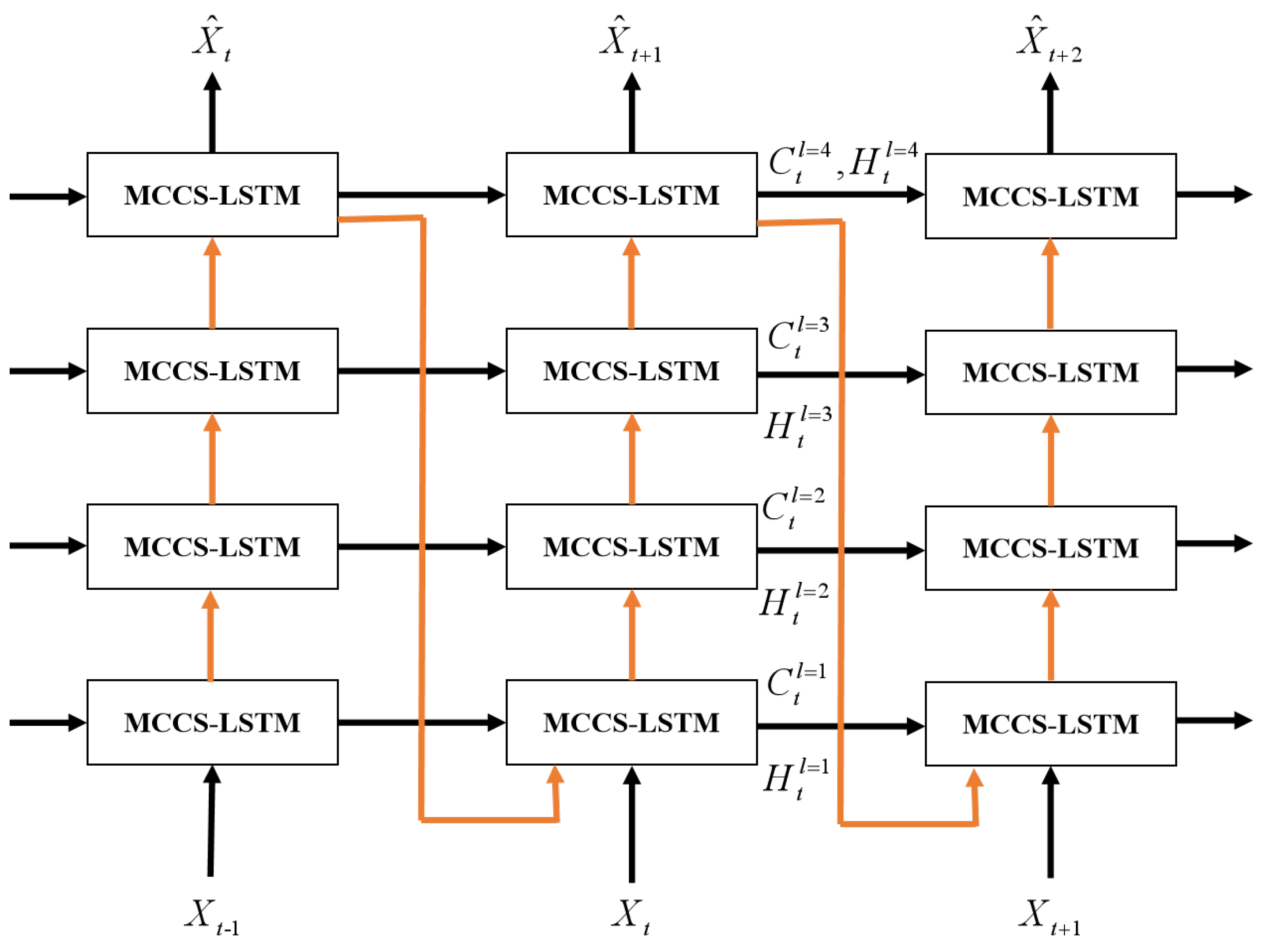
In the experiment, our model adopts a 4-layer MCCS-LSTM network with each layer containing 128 hidden states and 5 × 5 kernels. The parameter settings of the experiment are shown in

Table 1. Parameter Settings.

Learning Rate	Batch Size	Patch Size	Optimizer
0.001	8	4	Adam

. Setting the initial learning rate to 0.001, mini-batch to 8, and patch size to 4. In addition, planned sampling [20] is adopted, mean square error is used as the loss function, and all models are trained by the ADAM optimizer [21].

Before training, all radar echo maps were normalized to [0, 1] as the input, and we use NVIDIA P100 GPU to train and test based on Pytorch.

4.2. Experimental Results

Table 2. Comparison results of some models South of CIKM dataset in terms of Heidke Skill Score (HSS) and Critical Success Index (CSI). Bold denotes the best evaluate index among all models.

dBZ Threshold	CSI				HSS
	10	20	30	avg	10	20	30	avg
ConvLSTM	0.6943	0.4601	0.1963	0.4503	0.6937	0.5401	0.2630	0.4989
PredRNN	0.6907	0.4708	0.2036	0.4550	0.6916	0.5526	0.2731	0.5058
PredRNN++	0.6905	0.4631	0.2079	0.4538	0.6963	0.5521	0.2793	0.5092
MIM	0.6906	0.4571	0.1965	0.4481	0.6892	0.5402	0.2646	0.4980
IDA-LSTM	0.6947	0.4617	0.2085	0.4549	0.6958	0.5420	0.2777	0.5051
MCCS-LSTM	0.7001	0.4777	0.2188	0.4656	0.7006	0.5592	0.2919	0.5173

shows all results on CIKM dataset. Here, in addition to the MCCS-LSTM model proposed in this paper, ConvLSTM, PredRNN, PredRNN++, MIM, IDA-LSTM were applied and tested. All models used the same training set, validation set and test set. we adopted a random mechanism to initialize the weights of models and chose the best by training each model several times.

From the above table, our model achieves the best performance under three threshold, and the advantage of our model becomes increasingly obvious as threshold increases. To better illustrate the results, we visualize some qualitative results in Figure 7.

As can be observed from Figure 7, our model not only can accurately predict the boundaries, but also can achieve better timeliness. All the above results demonstrate that our model improves the prediction accuracy.

In order to test the predictive effect in the longer time range, we conduct some experiments on Guangdong Province of China radar dataset.

Table 3. Comparison results of some models in terms of Heidke Skill Score (HSS) and Critical Success Index (CSI). Bold denotes the best evaluate index among all models.

dBZ Threshold	CSI				HSS
	10	20	30	avg	10	20	30	avg
ConvLSTM	0.5936	0.4285	0.2050	0.4090	0.7073	0.5528	0.3057	0.5219
PredRNN	0.5685	0.4286	0.2685	0.4219	0.6836	0.5498	0.3764	0.5366
PredRNN++	0.5291	0.4387	0.2489	0.4266	0.7061	0.5625	0.3547	0.5411
MIM	0.5968	0.4436	0.2546	0.4317	0.7097	0.5653	0.3564	0.5438
IDA-LSTM	0.5951	0.4445	0.2345	0.4247	0.7070	0.5642	0.3330	0.5347
MCCS-LSTM	0.5989	0.4576	0.2466	0.4344	0.7117	0.5841	0.3573	0.5510

shows the experimental results using different models. Here, in addition to the MCCS-LSTM model proposed in this paper, ConvLSTM, PredRNN, PredRNN++, MIM, IDA-LSTM were applied and tested on the data set. All models used the same training set, validation set and testing set. we adopted a random mechanism to initialize the weights of models and choose the best by training each model several times.

From the above table, it can be seen under three threshold, the MCCS-LSTM model we proposed achieves the best performance in terms of the HSS, CSI. Although when the threshold is 30, PredRNN performs best. One of the reason for this result is that as the reflectivity threshold increases, the filtered information also increases synchronously, resulting in poor prediction effect. Furthermore, the other reason is that the high echo area changes quickly, our model is slightly weaker than PredRNN in capturing short-term dynamics. However, according to the overall average results, our model is better than other models. When the threshold value is 20, the CSI of MCCS-LSTM model is 2.9% higher than that of IDA-LSTM model, and the HSS of MCCS-LSTM model is 3.2% higher than that of MIM model, which effectively improves the accuracy of radar echo extrapolation. The results of PredRNN++ and MIM are better than those of ConvLSTM, PredRNN and IDA-LSTM. ConvLSTM performs the worst among all these models. Although on the whole testing set, the differences between different models are small, the difference is obvious in a single sample. Therefore, these differences can reduce economic losses in a specific precipitation event. Considering that the time series is a whole, it is more scientific to use the mean value on testing set.

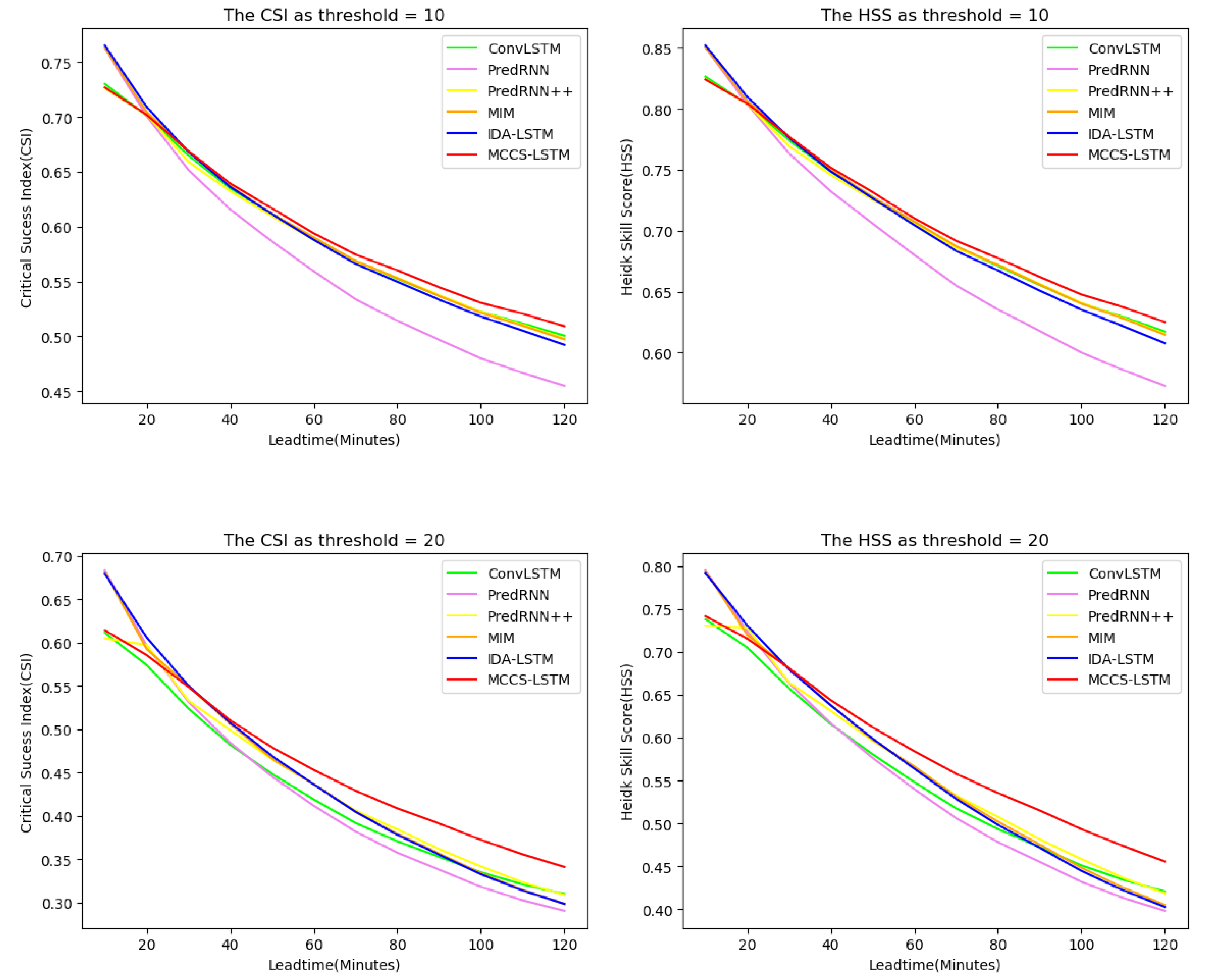
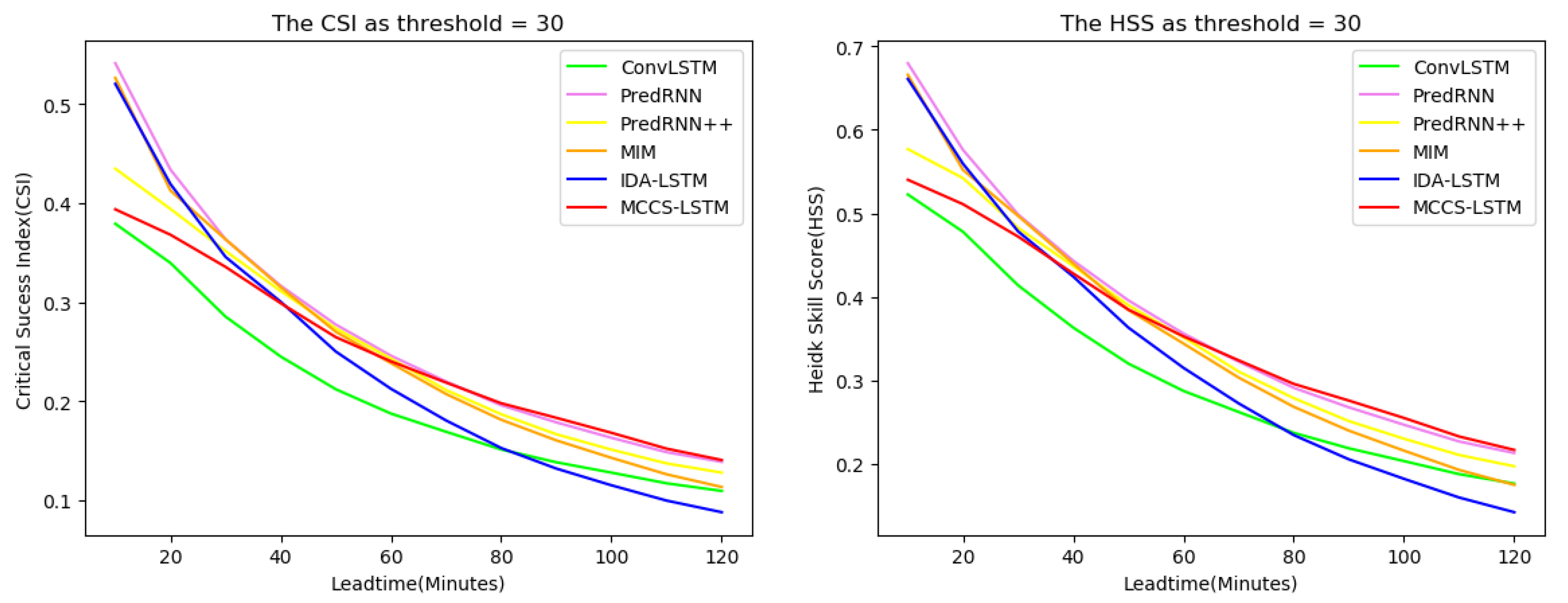
In the whole testing set, we drew Figure 8 to show the CSI and HSS change curves of all models at each time stamps. As can be seen from the figure, when the threshold is 10, 20, and 30, except for the first few time stamps, our model is superior to other models in CSI and HSS. This is because our model pays more attention to context information and has weak ability to extract abrupt features. Besides, when the threshold is 20, our model achieves effective prediction particularly in the last few time stamps compared to other models. In addition, ConvLSTM and PredRNN perform worst at threshold 20. It shows that our method can significantly improve the prediction accuracy with longer lead times, which is particularly important educing the harm of severe convective weather to the human economy and society. In fact, it thanks to our model which can effectively aggregate contextual information and capture the long-term dependencies.

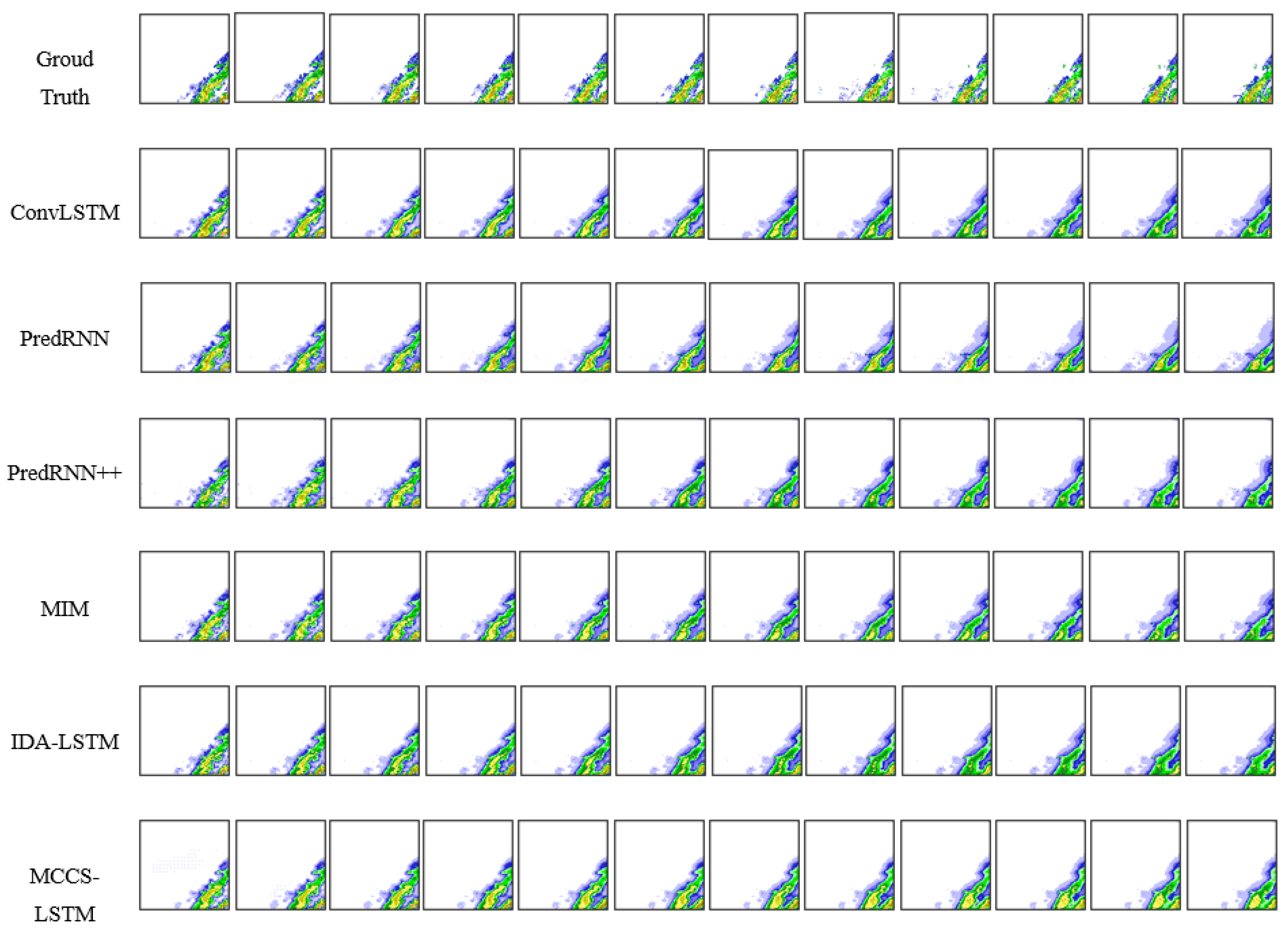
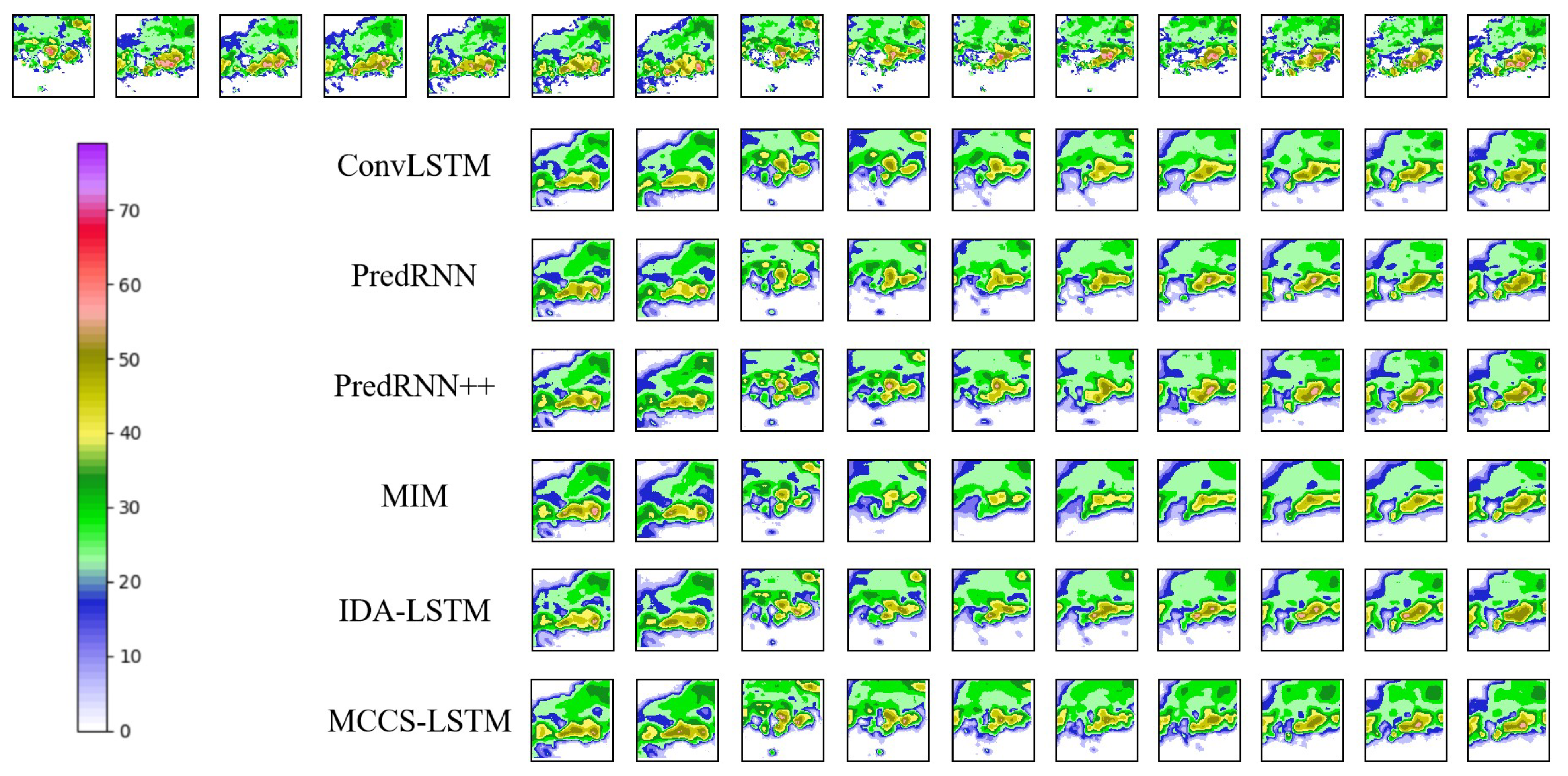
In order to compare the experimental results better, we visualized the extrapolation results of the radar echo from 4:50–6:50 a.m. on 31 August 2020 in Guangdong Province of China radar dataset, as shown in Figure 9. It can be seen from the figure that as the prediction time becomes longer, the extrapolation results of ConvLSTM, PredRNN++, MIM and IDA-LSTM models gradually became fuzzy, the high echo area gradually became smaller or even disappeared, and the whole prediction boundary area also gradually smoothen. PredRNN and MCCS-LSTM can well retain the high echo area, but compared with PredRNN, MCCS-LSTM can better retain the details of prediction results, which is due to the structure of MCCS-LSTM that can effectively transmit context information. This makes it able to capture the short-term dependencies between adjacent frames and retain the long-term dependencies of the entire echo sequence.

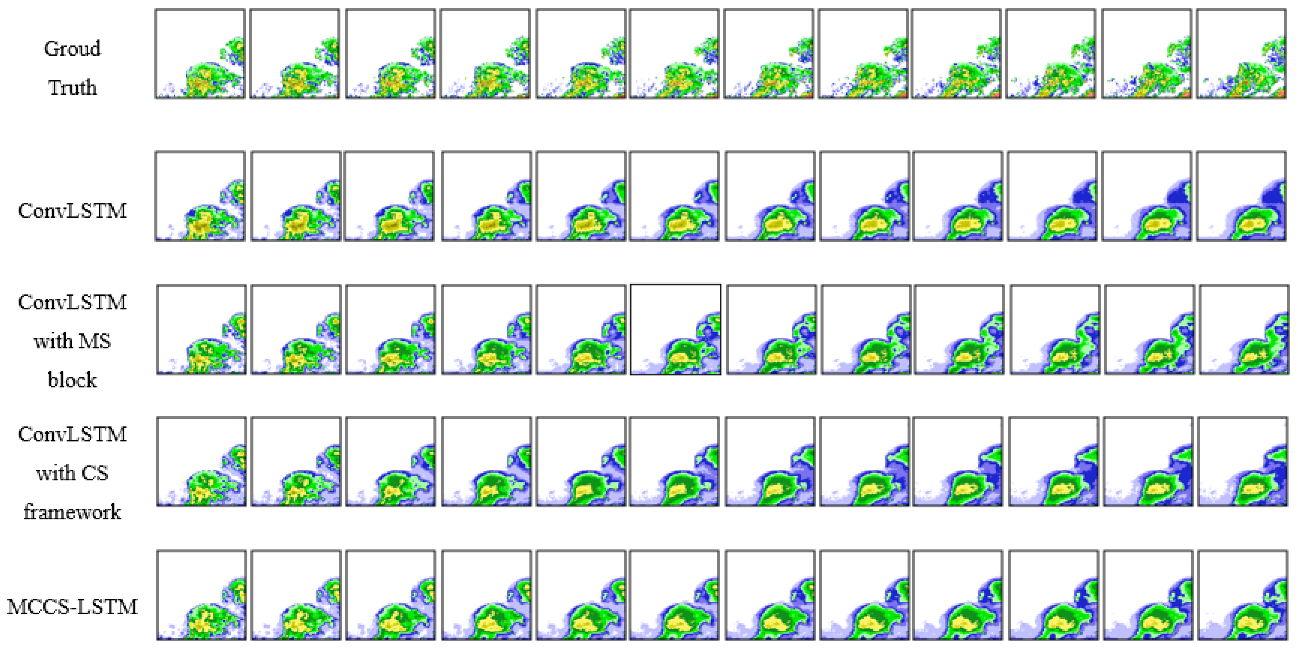
4.3. Ablation Study

In order to further investigate the effectiveness of CS framework and MS block, we conducted ablation experiments. On the basis of ConvLSTM, CS Framework and MS Block were separately added to ConvLSTM, and then they are compared with ConvLSTM and our model MCCS-LSTM. The experimental results are shown in

Table 4. Comparison results of Ablation study experiment in terms of Critical Success Index (CSI) and Heidke Skill Score (HSS). Bold denotes the best evaluate index.

dBZ Threshold	CSI				HSS
	10	20	30	avg	10	20	30	avg
ConvLSTM	0.5936	0.4285	0.2050	0.4090	0.7073	0.5528	0.3057	0.5219
ConvLSTM with MS block	0.5764	0.4290	0.2404	0.4152	0.6906	0.5512	0.3450	0.5289
ConvLSTM with CS framework	0.5792	0.4317	0.2247	0.4119	0.6932	0.5533	0.3241	0.5235
MCCS-LSTM	0.5989	0.4576	0.2466	0.4344	0.7117	0.5841	0.3573	0.5510

.

Table 4 shows that ConvLSTM with MS block and ConvLSTM with CS framework perform better than ConvLSTM, and ConvLSTM with both CS framework and MS block (MCCS-LSTM) delivers the best results. So the results validate the effectiveness of CS framework and MS block. Overall, ConvLSTM with MS block performs better than ConvLSTM with CS framework.

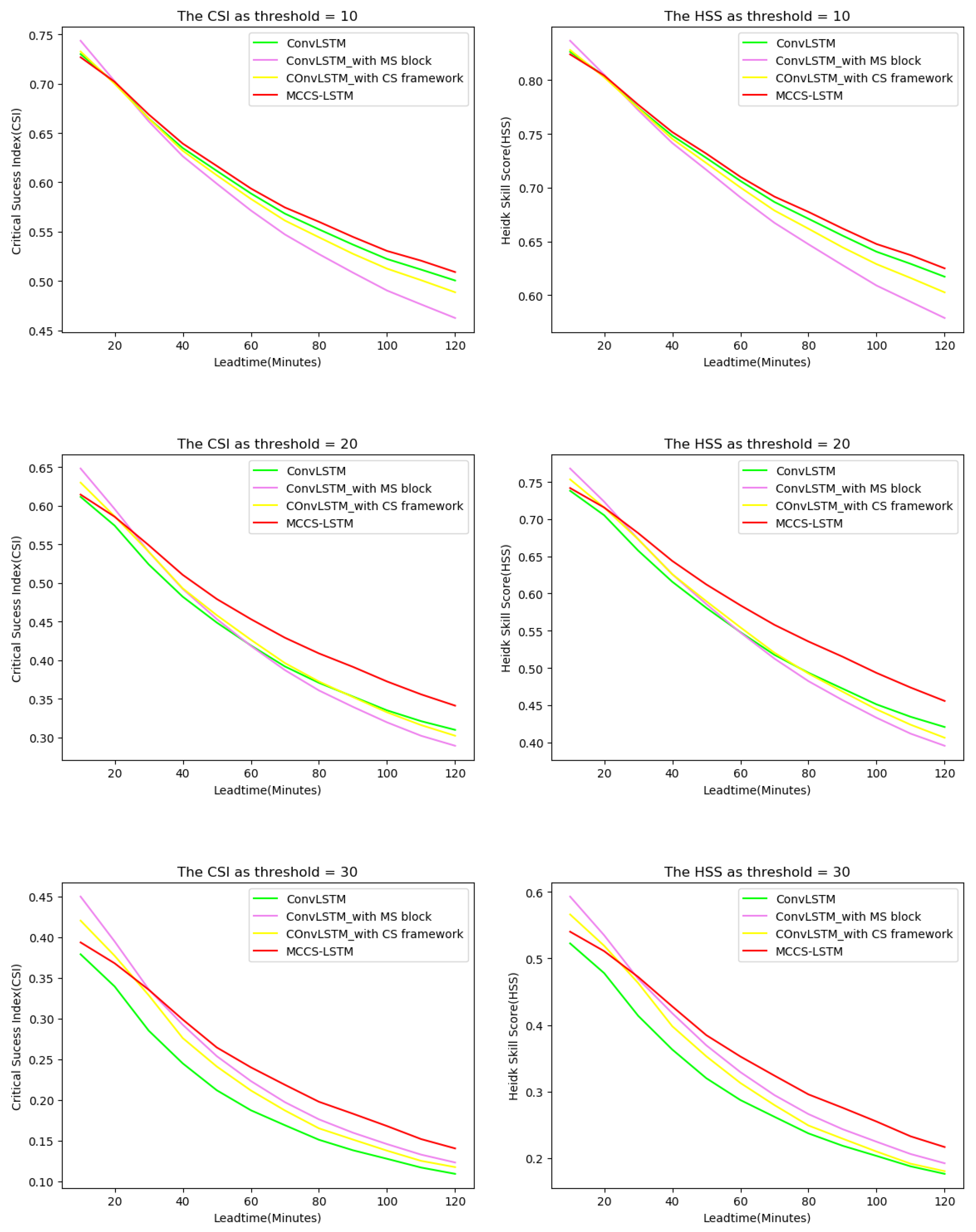
Similarly, we also depict the HSS and CSI curves changes at different lead times in Figure 10. It can be seen from the figure that as the prediction lead time becomes longer, the advantages of our model become more and more obvious. This thanks to our model by having the ability to build the long-term dependency and the short-term dependency effectively. In summary, CS Framework and MS block both play positive roles to predict longer lead time, which are profitable for economic society.

In order to visually compare the experimental results of removing CS framework and MS block, we visualized the extrapolation results of radar echo from 11:40–13:40 a.m. on 12 August 2020 in South China, as shown in Figure 11. We can see that the extrapolated result of ConvLSTM is gradually smoothed, and some areas tend to fade away. The model of MS block can retain the contour feature of radar map. The model of CS framework can effectively predict the variation trend of the high echo value regions.

In summary, the ablation studies further verifies the validity of MS block and CS framework, and the effectiveness of predicting radar echo movement in a longer lead time.

5. Discussion

Firstly, we discussed the positive effect of capturing the full-image dependencies in feature map. In a specific area, the weather system at each position is related. Specifically, there are dependencies between each pixels in radar echo map. From Figure 10, we can see the MS block effectively found the relationship between each pixels, providing improved forecast quality. This is a great significance for the accurate prediction of strong convective weather in some important areas. We therefore believe that capturing full-image dependence is a breakthrough to improve the effect of radar echo extrapolation in the future. Futhermore, we argued that using more complicated techniques in deep learning can be more effective to capture full-image dependency such as the Feature Integration Unit (FIU) [22] technology.

Secondly, we noticed that our model did not perform as well as some models in the first few lead times in Figure 7. After the experiment and comparision, we argued that the criss-cross attention used in MS block probably exists the problem of predicting the high radar echo areas in the first few lead times. However, our model seemed to be more stable in predicting medium radar echo areas. Therefore integrating some existing methods to improve the predict quality of high radar echo value parts is our future work. Besides, from Table 2, we can see that the performance of PredRNN is better than other models. By comparing these models based on radar echo extrapolation literature, we noticed that the external memory of PredRNN plays an important role in exploring new features, such as the generation of high radar echo areas. The variation trend of high intensity echo area is relatively fast. In the future, in order to improve the nowcasting in some extreme weather events, we will explore to improve our model’s ability of capturing short-term dynamics.

Finally, precipitation system processes exhibit complex non-stationarity in space and time. Therefore, it is very difficult to achieve accurate prediction. According to the limited lifetime of radar echo, we cannot accurately predict the evolution trend of radar echo based on only radar data. In the future, we will consider introducing some meteorological elements into extrapolation model to improve the prediction.

6. Conclusions

In this paper, we propose a new radar echo extrapolation model named MCCS-LSTM. To capture the long-term and short-term dependencies on radar echo movement, we put forward context sensing framework and multi-scale spatiotemporal block with criss-cross attention. Experiments show that MCCS-LSTM can effectively mitigate the radar echo map blurring and improve prediction accuracy with longer prediction lead times. The effectiveness of our model is fully proved by the experimental comparison of existing models. In the future, we will study the radar echo prediction with longer time duration (0–6 h in the future), and improve the forecasting ability for precipitation nowcasting.

References

1. Shi, E.; Li, Q.; Gu, D.; Zhao, Z. A method of weather radar echo extrapolation based on convolutional neural networks. In Proceedings of the International Conference on Multimedia Modeling, Bangkok, Thailand, 5–7 February 2018; pp. 16–28. [Google Scholar]
2. Xingjian, S.; Chen, Z.; Wang, H.; Yeung, D.Y.; Wong, W.K.; Woo, W.C. Convolutional LSTM network: A machine learning approach for precipitation nowcasting. In Advances in Neural Information Processing Systems; The MIT Press: Cambridge, MA, USA, 2015; pp. 802–810. [Google Scholar]
3. Marshall, J.S.; Palmer, W. The distribution of raindrops with size. J. Meteor. 1948, 5, 165–166. [Google Scholar] [CrossRef]
4. Sokol, Z.; Mejsnar, J.; Pop, L.; Bližňák, V. Probabilistic precipitation nowcasting based on an extrapolation of radar reflectivity and an ensemble approach. Atmos. Res. 2017, 194, 245–257. [Google Scholar] [CrossRef]
5. Pop, L.; Sokol, Z.; Minářová, J. Nowcasting of the probability of accumulated precipitation based on the radar echo extrapolation. Atmos. Res. 2019, 216, 1–10. [Google Scholar] [CrossRef]
6. LeCun, Y.; Bengio, Y.; Hinton, G. Deep learning. Nature 2015, 521, 436–444. [Google Scholar] [CrossRef] [PubMed]
7. Wang, Y.; Long, M.; Wang, J.; Gao, Z.; Yu, P.S. Predrnn: Recurrent neural networks for predictive learning using spatiotemporal lstms. In Proceedings of the 31st International Conference on Neural Information Processing Systems, Long Beach, CA, USA, 4–9 December 2017; pp. 879–888. [Google Scholar]
8. Wang, Y.; Gao, Z.; Long, M.; Wang, J.; Philip, S.Y. Predrnn++: Towards a resolution of the deep-in-time dilemma in spatiotemporal predictive learning. In Proceedings of the International Conference on Machine Learning, PMLR, Stockholm Sweden, 10–15 July 2018; pp. 5123–5132. [Google Scholar]
9. Wu, K.; Shen, Y.; Wang, S. 3D convolutional neural network for regional precipitation nowcasting. J. Image Signal Process. 2018, 7, 200–212. [Google Scholar] [CrossRef]
10. Wang, Y.; Zhang, J.; Zhu, H.; Long, M.; Wang, J.; Yu, P.S. Memory in memory: A predictive neural network for learning higher-order non-stationarity from spatiotemporal dynamics. In Proceedings of the IEEE/CVF Conference on Computer Vision and Pattern Recognition, Long Beach, CA, USA, 15– 20 June 2019; pp. 9154–9162. [Google Scholar]
11. Luo, C.; Li, X.; Wen, Y.; Ye, Y.; Zhang, X. A Novel LSTM Model with Interaction Dual Attention for Radar Echo Extrapolation. Remote Sens. 2021, 13, 164. [Google Scholar] [CrossRef]
12. Chen, L.C.; Papandreou, G.; Kokkinos, I.; Murphy, K.; Yuille, A.L. Deeplab: Semantic image segmentation with deep convolutional nets, atrous convolution, and fully connected crfs. IEEE Trans. Pattern Anal. Mach. Intell. 2017, 40, 834–848. [Google Scholar] [CrossRef] [PubMed] [Green Version]
13. Chen, L.C.; Yang, Y.; Wang, J.; Xu, W.; Yuille, A.L. Attention to scale: Scale-aware semantic image segmentation. In Proceedings of the IEEE Conference on Computer Vision and Pattern Recognition, Las Vegas, NV, USA, 27–30 June 2016; pp. 3640–3649. [Google Scholar]
14. Huang, Z.; Wang, X.; Huang, L.; Huang, C.; Wei, Y.; Liu, W. Ccnet: Criss-cross attention for semantic segmentation. In Proceedings of the IEEE/CVF International Conference on Computer Vision, Seoul, Korea, 27–28 October 2019; pp. 603–612. [Google Scholar]
15. Melis, G.; Kočiskỳ, T.; Blunsom, P. Mogrifier lstm. arXiv 2019, arXiv:1909.01792. [Google Scholar]
16. Zhao, T.; Wu, X. Pyramid feature attention network for saliency detection. In Proceedings of the IEEE/CVF Conference on Computer Vision and Pattern Recognition, Long Beach, CA, USA, 16–17 June 2019; pp. 3085–3094. [Google Scholar]
17. Mei, Y.; Fan, Y.; Zhang, Y.; Yu, J.; Zhou, Y.; Liu, D.; Fu, Y.; Huang, T.S.; Shi, H. Pyramid attention networks for image restoration. arXiv 2020, arXiv:2004.13824. [Google Scholar]
18. Schaefer, J.T. The critical success index as an indicator of warning skill. Weather. Forecast. 1990, 5, 570–575. [Google Scholar] [CrossRef] [Green Version]
19. Hogan, R.J.; Ferro, C.A.; Jolliffe, I.T.; Stephenson, D.B. Equitability revisited: Why the “equitable threat score” is not equitable. Weather. Forecast. 2010, 25, 710–726. [Google Scholar] [CrossRef] [Green Version]
20. Geng, H.; Wang, T. Spatiotemporal Model Based on Deep Learning for ENSO Forecasts. Atmosphere 2021, 12, 810. [Google Scholar] [CrossRef]
21. Kingma, D.P.; Ba, J. Adam: A method for stochastic optimization. arXiv 2014, arXiv:1412.6980. [Google Scholar]
22. He, Z.; Liu, K.; Liu, Z.; Dou, Q.; Yang, X. A lightweight multi-scale feature integration network for real-time single image super-resolution. J. Real-Time Image Process. 2021, 18, 1221–1234. [Google Scholar] [CrossRef]
Figure 1. Structure of ConvLSTM.
Atmosphere 13 00192 g001
Figure 2. The mechanism of criss-cross attention.
Atmosphere 13 00192 g002
Figure 3. The structure of context sensing framework.
Atmosphere 13 00192 g003
Figure 4. Multi-Scale Spatiotemporal block (MS block) with criss-cross attention.
Atmosphere 13 00192 g004
Figure 5. The inner structure of MCCS-LSTM unit.
Atmosphere 13 00192 g005
Figure 6. The architecture of MCCS-LSTM model.
Atmosphere 13 00192 g006
Figure 7. The prediction results for echo on CIKM dataset. The first row refers to real observations, the top five images indicates the input. Other rows represent prediction results of different models, respectively.
Atmosphere 13 00192 g007
Figure 8. The performance changes against different nowcasting lead time in terms of CSI and HSS. The three rows represent, respectively, CSI and HSS curve changes over the threshold of 10, 20 and 30—best view in color.
Atmosphere 13 00192 g008aAtmosphere 13 00192 g008b
Figure 9. The prediction results for echo in Guangdong Province of China, 31 August 2020, 4:50 UTC. The images in the first row are the ground-truth output, a total of 12 radar echo maps, denoting the forecast results for the next two hours. Other rows are the prediction of some methods.
Atmosphere 13 00192 g009
Figure 10. The performance changes against different nowcasting lead time in ablation experiments in terms of CSI and HSS. (Best view in color).
Atmosphere 13 00192 g010
Figure 11. The prediction results of ablation studies on an example (Best view in color).
Atmosphere 13 00192 g011