Article

Plausible Precipitation Trends over the Large River Basins of Pakistan in Twenty First Century

1
NUST Institute of Civil Engineering (NICE), School of Civil and Environmental Engineering (SCEE), National University of Sciences and Technology (NUST), Islamabad 44000, Pakistan
2
Civil Engineering Department, University of Engineering and Technology, Lahore 420000, Pakistan
3
Department of Geoinformatics—Z_GIS, Faculty of Digital and Analytical Sciences, Paris Lodron University of Salzburg, Schillerstraße 30, 5020 Salzburg, Austria
4
Department of Geosciences, University of Arkansas, Fayetteville, AR 72701, USA
*
Author to whom correspondence should be addressed.
Atmosphere 2022, 13(2), 190; https://doi.org/10.3390/atmos13020190
Submission received: 16 November 2021 / Revised: 11 January 2022 / Accepted: 18 January 2022 / Published: 24 January 2022

Abstract

:
Inter alia, inter-annual and spatial variability of climate, particularly rainfall, shall trigger frequent floods and droughts in Pakistan. Subsequently, a higher proportion of the country’s population will be exposed to water-related challenges. This study analyzes and projects the long-term spatio-temporal changes in precipitation using the data from 2005 to 2099 across two large river basins of Pakistan. The plausible precipitation data to detect the projected trends seems inevitable to study the future water resources in the region. For, policy decisions taken in the wake of such studies can be instrumental in mitigating climate change impacts and shape water management strategies. Outputs of the Coupled Model Intercomparison Project 5 (CMIP5) climate models for the two forcing scenarios of RCP 4.5 and RCP 8.5 have been used for the synthesis of projected precipitation data. The projected precipitation data have been synthesized in three steps (1) dividing the area in different climate zones based on the similar precipitation statistics (2) selection of climate models in each climate zone in a way to shrink the ensemble to a few representative members, conserving the model spread and accounting for model similarity in a baseline period of 1971–2004 and the projected period of 2005–2099 and (3) combining the selected model’s data in mean and median combinations. The future precipitation trends were detected and quantified, for the set of four scenarios. The spatial distribution of the precipitation trends was mapped for better understanding. All the scenarios produced consistent increasing or decreasing trends. Significant declining trends were projected in the warm wet season at 0.05% significance level and the increasing trends were projected in cold dry, cold wet and warm dry seasons. Framework developed to project climate change trends during the study can be replicated for any other area. The study therefore can be of interest for researchers working on climate impact modeling.

1. Introduction

Pakistan underwent recurring flooding during 1988, 1992, 2010, 2013, and 2014 in the Upper Catchments of Indus, Jhelum, and Chenab Rivers. Intense and devastating floods that increase fatalities and massive infrastructural damage have become somewhat annual routine in the country. Especially, heavy monsoon rains that hit the country from July to September due to the varying meteorological situations are major contributors to extreme monsoonal flooding [1,2]. Therefore, flood disaster mitigation and hazard management have become the point of concern for all stakeholders.
The intensity, variability, and frequency of temperature, floods, droughts, cyclones, and precipitation may exhibit substantial variations, thus presenting evidence of the impacts of climate change in Pakistan [3]. Northern Pakistan is the junction of three world-renowned mountain ranges known as the Karakoram, the Himalayas, and the Hindukush, producing the third largest mass of ice after the Polar Regions, located in the northern hemisphere. Westerly waves and Monsoon lows from the Mediterranean Sea, seasonal lows from the Arabian Sea, and depression caused by low pressures from the Bay of Bengal impact Pakistan [4]. The widespread perception is that this trend is part of a larger climate change phenomenon that has accelerated the hydrological cycle.
The climatic variability as a result of natural mechanisms of oceans, atmosphere, land surface, and anthropogenic forces is simulated by Global Circulation Models, commonly known as GCMs. These are the multi-dimensional numerical models, which follow the law of conservation of mass, momentum, and energy, representing the climate system. GCMs include numerous parameters related to atmospheric circulations, feedback mechanisms, moisture and wind fluxes, earth’s rotational effects, and thermodynamics. Each model tends to simulate some aspects of the climate system well and some others not so well, leading to overestimation or underestimation of climate variables [5]. Therefore, these factors lead to different outputs for different GCMs with the same forcing scenarios for future projections [6,7,8,9,10]. The research question of the present study is how to use a variety of GCMs’ outcomes to obtain plausible meteorological inputs for the climate change impact modeling for the study area, having spatiotemporal heterogeneous climate.
Many studies have consistently demonstrated that the selection of GCMs, for assessing climate change impacts, is the main contributor to uncertainty in the assessments of hydrological response to climate change. This has been proved by quantifying and comparing the uncertainties originating from different sources such as inherent errors in GCMs, forcing scenarios, downscaling and bias correction techniques, and hydrological models’ parameters [11]. The Intergovernmental Panel on Climate Change [12] has proposed several GCM selection criteria such as using the latest version of GCMs’ simulations, GCMs’ with high temporal and spatial resolution, GCMs’ producing high end and low-end climate signals [13,14], commonly known as an envelope-based selection method, or GCMs presenting realism of historical/baseline simulations [15,16].
The lack of realism of baseline simulations of some models cannot be linked with the plausibility of model projections. The correlation between past performance and future prediction is very weak; it means that model performance based on the historical period data may not be valid in an uncertain future climate [17,18,19]. It is necessary to consider the non-negligible probability of all the projections to use for future climate change detection, decision making, and planning [19]. Thus, the use of a multi-model ensemble (MME) is advocated and recommended over an individual model to synthesize the meteorological inputs for the climate change impact studies [20,21]. They should be synthesized, in a way to represent the full range of climate variability signals, from the available GCMs, for plausible future climate projections [22]. The subjective approach of past performance-based selection should only be used when severely unrealistic models that are not reliable for the future prediction have to be removed [14]. To attain unbiased distribution of the projected climate data, the selection of the GCMs in an ensemble should be in such a manner that they are not interdependent/correlated to each other. The correlated models gain too much weight in the larger MME [18]. The high correlation between the GCMs in the MME is responsible for the biases in the assessment of climate change impacts. It is imperative to provide the solution of biases of large MME by reducing its size using a smaller number of climate models with minimum loss of information. Effective small sub-ensembles are developed from an ensemble with a large number of models having more extensive dependencies on each other [23,24].
It is usual in the climate research community to compare or assess the spatial areal average of the climate data for selecting GCMs using any of the three methods of past performance, envelope-based approaches, and hybrid method [13,16]. This spatial average may not represent the local variances in spatial and temporal climate characteristics. Thus, strong consideration of this variation in spatial climatic conditions is required for the plausible ecological projections. To continue with the selection of a GCM for climate change impact studies, the area should be considered climatically homogeneous. The formation of homogeneous climatic zones [25] allows for a better understanding of the complex spatiotemporal variability of precipitation across an area. These climate zones are delineated using the spatial similarity/homogeneity of the precipitation statistics in an area using the dense data network.
Precipitation being the most provocative variable in terms of climate change impacts, studies have been conducted to estimate precipitation trends in various parts of Pakistan using best performing GCMs [26], single or two GCMs [27,28,29], hierarchical Bayesian Spatio-temporal methods [30], projections of trend line [31], artificial neural network (ANN) and Support vector regression (SVM) models [32]. Our confidence deficit in discounting any projections with a lack of realism of baseline simulations leads to the application of a novel framework of climate model selection. This framework focuses on (1) the delineation of the sub-regions having the stations with similar precipitation characteristics named as climate zone (2) selection of the climate models, based on climate signals spread in each climate zone for the possible future bandwidth of the climate change trends (3) combining the range of precipitation projections outcomes from the selected models for two climate forcing scenarios of RCP4.5 and RCP 8.5 (4) precipitation change trend detection. The selection of GCMs, from the large MME, was carried out by the formation of clusters of correlated GCMs and selecting the high and low-end producers of climate signals in each cluster in a climate zone. Therefore, a smaller MME of GCMs was formed with the larger ensemble characteristics. The daily data of the member GCMs of each MME were then combined in two ways: mean and median to investigate the future climate trend [33]. We intended to combine information from the GCMs to provide a set of scenarios for the study area that represent the uncertainty range in a credible manner. The precipitation trends were then detected for all those scenarios. The study also highlights the significance of machine learning clustering algorithms of supervised learning, for the pattern detection and grouping of long-term climate data of high temporal scale in a large study area. Subsequently, the research community is prompted to develop a framework that could analyze and predict the impacts of climate change and augment the decision support systems for a sustainable future. Moreover, the recurring demand for such research has also increased among policy-making circles and public pressure groups. Challenges such as food shortage and shelter insecurities are closely knitted with environmental degradation factors, such as floods, rising sea levels, and global warming. Availability of reliable and updated climate data trends is thus a prerequisite to forge sound policies that can reduce implications of environmental degradation upon human lives.
Section 2 of the paper describes the study area and data used, which is followed by Section 3 that explains the methodology used. Section 4 presents the results, and lastly, conclusions are drawn in Section 5.

2. Study Area and Data
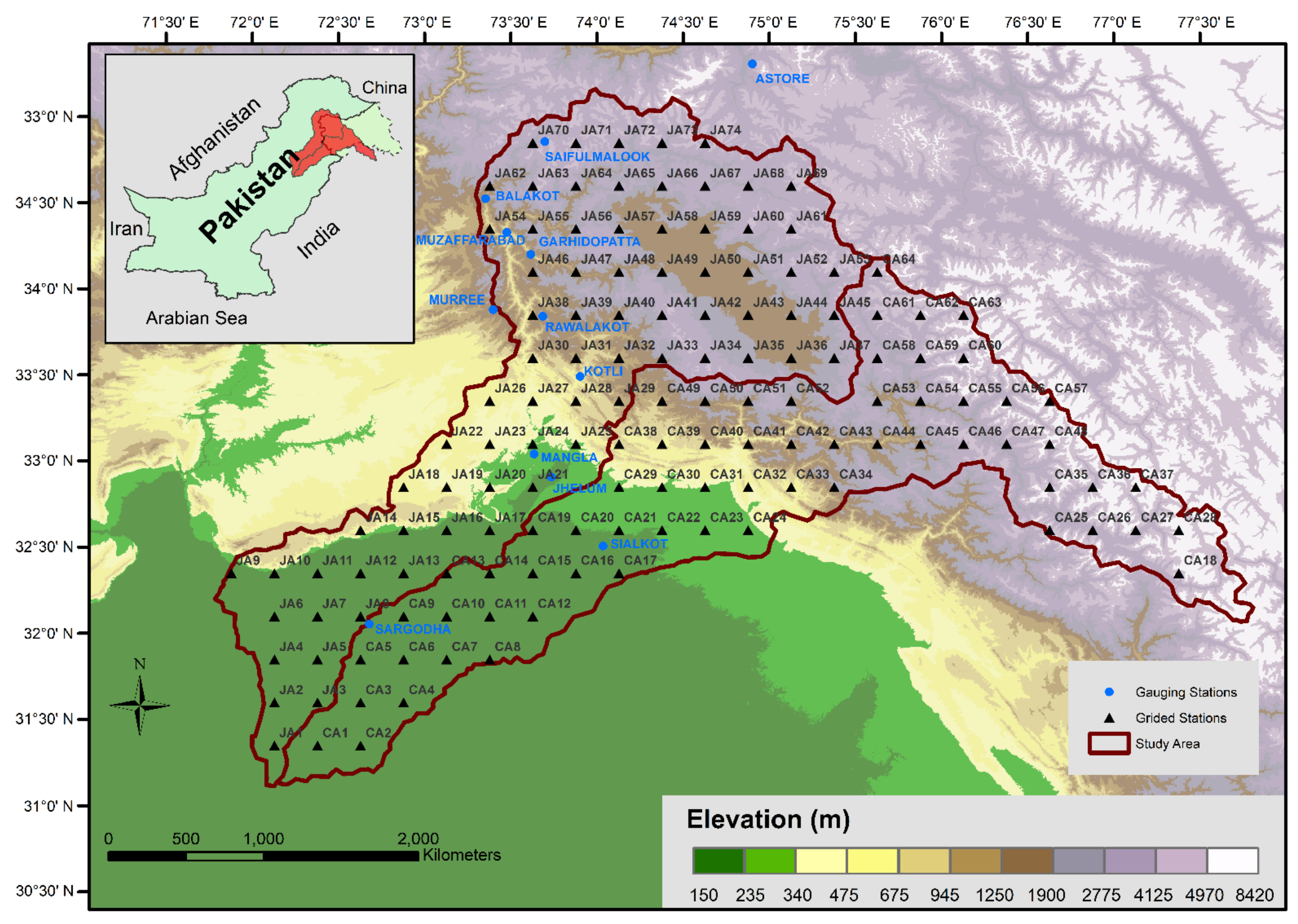
2.1. Study Area

The area under study is approximately 100,845 km2, which comprises two basins of Pakistan’s rivers, namely the Jhelum and Chenab. The altitude from the mean sea level varies between 146 and 6915 m. Figure 1 presents the digital elevation model and geographic location of the study area. The precipitation gauging stations and the points on which gridded data have been sampled is also shown in Figure 1. The westerly aggravations and the southwest monsoon are the major cause of 60% and 40% of the annual precipitation, respectively [16]. The variable climatic conditions depend upon the atmospheric circulation patterns, advected moisture, and a considerable range of variations in topography. The depleting water resources and recurrence of extreme events due to high hydro-climatic variability in the region have made it an important research arena.

2.2. Climatology

The westerly aggravations and the southwest monsoon are the major cause of 60% and 40% of the annual precipitation, respectively [16]. The variable climatic conditions depend upon the atmospheric circulation patterns, advected moisture, and a considerable range of variations in topography. The depleting water resources and recurrence of extreme events due to high hydro-climatic variability in the region have made it an important research arena. Seasonal precipitation in Pakistan is affected by weather systems of three types: the monsoon depressions originating from the Bay of Bengal cause summer precipitation [34], western disturbances emanate from the Mediterranean Sea are reasons for the winter precipitation [35], and tropical cyclones from the Arabian Sea in spring and fall [36]. In Pakistan, the monsoon season lasts from June to September, with the post-monsoon season lasting from October to November [37]. On examining the mean monthly historical precipitation in Jhelum and Chenab river basins [38,39,40], the seasons have been defined in the present study. The seasons are warm wet (July, August, and September) Cold Dry (October, November, and December), cold wet (January, February, and March), and warm dry (April, May, and June).
For warm wet season, the average total seasonal precipitation based on APHRODITE (1970–2004) varies from 140 mm to 230 mm in north and east of the study area, 440 mm to 1050 mm in the central region, and 160 mm to 230 mm in the southwest region.
For the cold dry season, the precipitation varies between 8.93 mm and 120 mm, minimum in southwest and maximum in north and east of the study area.
For the cold wet season, in the southwest region, it varies from 120 mm to 160 mm, in the central region 230 mm to 340 mm, and in the north and northeast region 160 mm to 340 mm.
For the warm dry season, in the southwest region 100 mm to 140 mm, and the central region 140 mm to 230 mm, and 140 mm to 250 mm in the north and southwest region.

2.3. APHRODITE Data

The trend of using the gridded climate data in the climate and hydrologic assessment studies has been increasing due to its easy accessibility and reliability. A reliable gridded data network of stations is required to divide the study area into the number of homogeneous climatic zones. The reliability of the Asian Precipitation—Highly Resolved Observational Data Integration Towards Evaluation of Water Resources (APHRODITE) dataset has been advocated by many previous studies [41,42,43] and it is considered as the best-gridded dataset available as of yet, for the high elevated mountainous areas of Asia [44]. There are many other gridded datasets available as an open-source e.g., European Reanalysis gridded dataset (ERA5) [45] and Global Meteorological forcing dataset for land surface Modelling (GMFD) [46]. ERA5 is also famous for its good resolution and accuracy. Our decision of using the APHRODITE product (V1101) [43] for the regionalization of the study area, was based on the comparative analysis of these three datasets in a study by Nusrat et al. [25]. In this study, monthly precipitation data of APHRODITE, ERA5 and GMFD were sampled at the 11 gauging stations, mentioned in Supplementary Materials Table S1. All these gauging stations are situated at different elevations. The three datasets were compared with the monthly observed precipitation data using the Kolmogorov Smirnov Test and Pearson Correlation Coefficient test. The criteria of better performance were based on a higher correlation coefficient and p-value of KS test more than 0.05 to reject the alternative hypothesis of a dissimilar probability distribution. The results suggested that the APHRODITE dataset is more reliable than the other two datasets at nearly all the gauging stations at different altitudes.

2.4. NEX-GDDP-GCMs-CMIP5 Data
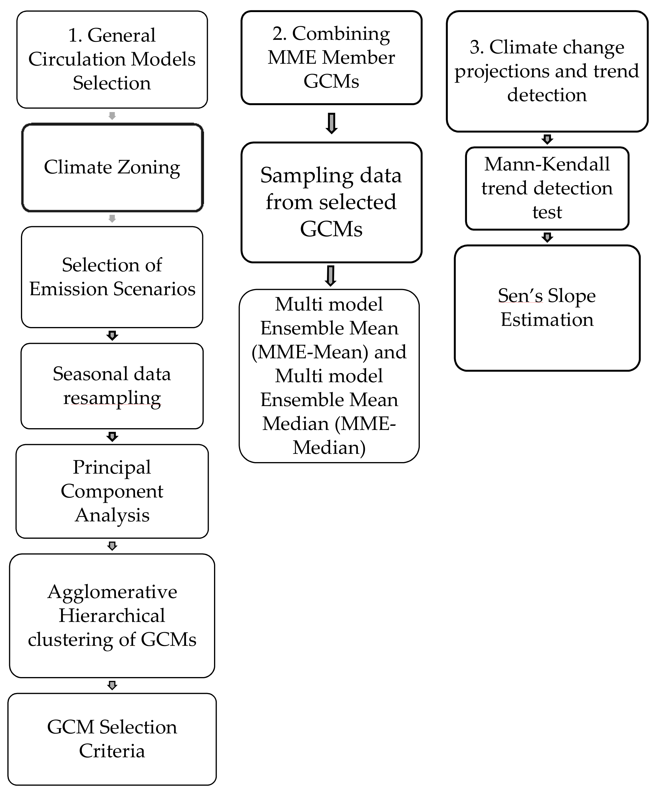
NASA Earth Exchange Global Daily Downscaled Projections (NEX-GDDP) dataset [47,48] has been used in this study for the historical and projected climate data. The outputs of the Coupled Model Intercomparison Project 5 (CMIP5) were used by National Aeronautics and Space Administration (NASA) to form NEX-GDDP. The list of 21 GCMs in the NEX-GDDP is provided in Supplementary Materials Table S1.
However, the CMIP5 experiments were meant to address the questions raised in the Assessment Report (AR4) of the Intergovernmental Panel on climate change IPCC [49]. Therefore, when fine-scale modeling is required, the climate impact modeling and Local-scale decision support system cannot rely on the coarser spatial resolution of CMIP5 GCMs. The NEX-GDDP dataset of 21 GCMs is downscaled to a finer resolution of 0.25° and bias-corrected using the bias-corrected spatial disaggregation method (BCSD) [47].
NEX-GDDP climate (maximum and minimum temperature and precipitation) datasets for the baseline period (1950–2005) and projected period (2005–2099) are publicly available. The projected data of CMIP5 GCMs have been bias-corrected and downscaled for the two forcing scenarios of representative concentration pathways (RCPs), i.e., RCP 4.5 and RCP 8.5, which were employed by IPCC for the fifth assessment report (AR5) [49].

3. Methodology

In this study, the Python module of Scikit–learn [50] has been used, assimilating many machine learning algorithms for supervised/unsupervised learning. The study area has been divided into different climate zones, of homogeneous climate, for each season, i.e., warm wet (July, August, and September), cold dry (October, November, and December), cold wet (January, February, and March) and warm dry (April, May, and June), following the methodology employed by [25].
With the help of Machine learning algorithms, large datasets of multivariate atmospheric parameters can easily be assessed and analyzed for the pattern/distribution variability study and impact modeling. Each step of the framework developed in this study has been translated into Python code. This framework of the study consists of three major steps (1) GCMs selection; (2) Combining the GCMs; and (3) climate change projections and trend detection. Figure 2 presents the flow chart of the methodology adopted in this study. Further details of all steps are discussed in the subsequent sections.

3.1. Climate Zoning

The first pre-requisite step in this framework is regionalization based on the climate of the region. Regionalization is the process of grouping the stations with homogeneous climate statistics and demarcating them into specific climate zones. For this process, long climate data records are required at various stations in the study area [51]. In the present study, the daily precipitation dataset of APHRODITE of 35 years was used for regionalization after its comparative performance evaluation with other gridded datasets.
There are various applications of regionalization of climate statistics e.g., in agricultural practices, hydrological extremes forecasting, and basin management [52]. The methods used to delineate climate regions are geographical convenience, subjective and objective partitioning [53,54]. In all these methods multivariate analysis techniques such as principal component analysis (PCA), correlation analysis, and clustering are widely used to demarcate the regions of homogeneous climate [55,56]. The geographical convenience method is an arbitrary and somewhat misleading approach based on the demarcation of the administrative boundaries. The subjective and objective partitioning methods are based on the demarcation of the region by grouping the meteorological sites having homogeneous climate statistics. The method employed for regionalization in the present study is agglomerative hierarchical clustering (AHC) of the principal components (PCs) of the precipitation data, at various stations of the region. Different Cluster validity indices were used to validate the number of clusters. The whole framework of regionalization step by step has been presented in the following sections.

3.1.1. Seasonal Data Resampling

The daily precipitation dataset of APHRODITE, at 138 Grid stations for the period 1975–2005, was sampled for hydrological seasons cycle: warm wet (July, August, and September), cold dry (October, November, and December), cold wet (January, February, and March) and warm dry (April, May, and June).

3.1.2. Principal Component Analysis (PCA)

The objective was to decrease the dimensions of the large matrix of the dataset of daily time series of 35 years for 138 grid stations. Principal Component Analysis (PCA) enabled us to reduce such a large matrix to a smaller sized matrix in addition to retaining as much descriptive of the data as possible. According to PCA, the data are projected onto different orthogonal axes which are called principal components. The symmetric covariance matrix is developed through the dataset, and then through the linear transformation technique principal components were identified. The eigenvectors depict the direction and the eigenvalues represent the magnitude of the extent of the axis or principal components representative of the data spread. The highly ranked principal components (PCs) which explained maximum cumulative variance in the dataset were identified through the scree plot and were used for the subsequent step. The component scores are derived by eigenvectors and the eigenvalues for all the stations in each PC. These component scores represent climate change patterns/signals in that specific site and may be considered an alternative to the meteorological parameters, which are statistically independent [14,55]. The function of scikit-learn [50] has been used to develop the code for the PCA.

3.1.3. Agglomerative Hierarchical Clustering (AHC)

Through this step, we were able to identify the clusters or groups of sites having similar climate signals. The climate change signals were estimated in the previous step of PCA, in the form of component scores. The component scores of the leading PCs were used in the clustering algorithm. The algorithm of Agglomerative Hierarchical Clustering [57,58] is an iterative process. It works on a bottom-up approach which starts from one point/self-cluster. Then, the size of the cluster keeps on increasing through nearest points one by one. In this way number of sequential combinations of clusters of the data points may be obtained. The optimum number of clusters is based upon the Euclidian distance [59] between the clusters. The dendrogram tree presents the meaningful information of different clusters and the Euclidian distances between the clusters, which forms the basis of the optimum number of clusters. The optimum number of clusters was determined with the help of cluster validity indices. Maximum Euclidian distance corresponding to the optimum number of clusters for each season was determined to truncate the dendrogram obtained through agglomerative clustering. Then number and identity of stations in each cluster were identified. The algorithm of scikit-learn [50] was used for agglomerative hierarchical clustering. The literature regarding different clustering techniques can be found in [14,60,61].

3.1.4. Formation of Climate Zones

There are different cluster validity tests, through which the number of clusters (NC) is decided. In the present study, the silhouette score (𝑆) [62] (described in Section 3.1.5) was used to determine the optimum number of clusters/groups of sites with statistically similar climates. The number and identity of the stations in each cluster were determined by truncating the dendrogram corresponding to Euclidian distance so that the estimated optimum number of clusters could be produced.
Different clusters of stations are plotted in the map of the study area in ArcGIS Tool (Environmental Systems Research Institute, Redlands, CA, USA). To enable a clearer presentation, regions are demarcated with the visible boundaries representing the climate zone. The reference station in each climate zone was selected based on the average climate signals of all the grid stations in the respective zone. The climate of the reference station is considered representative of the climate of the respective zone.

3.1.5. Silhouette Score

The Silhouette score [62] is calculated as the average of the Euclidian distances between the clusters. The number of clusters with maximum Silhouette Score is considered optimum. The Silhouette score (𝑆) can be calculated as
S = 1 N C i 1 n i r C i b r a r max b r , a r
and
a r = 1 n i 1 s C i , s r d r , s , b r = m i n j , j i 1 n j y C j d r , s ]
where NC is the symbol of the number of clusters; the ith cluster is represented by 𝐶𝑖 symbol for the number of objects in 𝐶𝑖 is 𝑛𝑖; the center of 𝐶𝑖 is denoted by 𝑐𝑖; and distance between r and s is denoted by 𝑑(r,s) [62].

3.2. GCM Selection in Climate Zones

The climate forcing scenarios, as four Representative Concentration Pathways (RCPs), have been used for AR5 by IPCC. These RCPs are RCP 2.6, a mitigation scenario; RCP4.5 and RCP6.0, scenarios of medium stabilization, and RCP8.5, high baseline emissions scenario [63]. We used RCP 4.5 and 8.5 future scenarios to cover the wide range of greenhouse gas emissions assumed in these scenarios. The projected daily precipitation data (2005–2099) of the selected GCMs in each climate were sampled for these forcing scenarios and combined with the mean and median for the projected climate trends. The selection of GCMs out of 21 CMIP5 GCMs was done using the daily precipitation data of historical (1971–2005) and projected period (2005–2099) at every reference station. We have illustrated the method using the example of GCMs selection in the ninth climate zone of the cold dry season for RCP 8.5. The climate zones for the cold dry season have been shown in Figure 3a, highlighting the ninth climate zone in the study area. The steps are as follows:
  • For the projected period, the precipitation data were sampled for two forcing scenarios, RCP 4.5 and RCP 8.5. The set of GCMs was selected using each of the forcing scenarios separately. It means that each climate zone would have two sets of selected GCMs, each corresponding to one forcing scenario. The idea was to incorporate every possible spread and diversity of climate signals to select GCMs, which is the basis of the envelope-based selection approach.
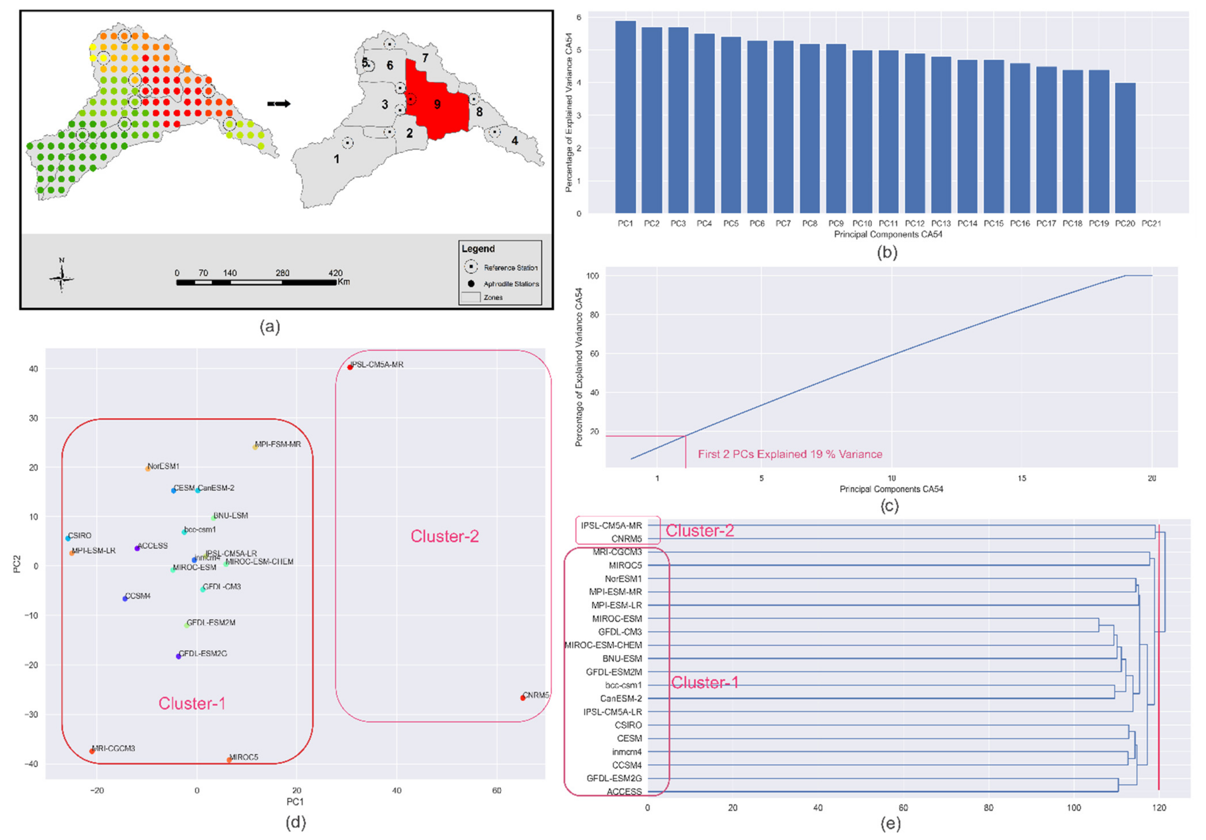
  • After combining the data of 21 GCMs for the historical and projected periods for RCP 4.5 and RCP 8.5 for all the reference stations, Principal Component Analysis (PCA) was performed on 21 GCMs data at each of the reference stations. The objective was to reduce the dimensions of the large matrix of the daily time series of 129 years (base period: 1971–2004 and projected period: 2005–2099) for the reference stations in each of the climate zone of every season. In addition, to retain as much descriptive of the data as possible, PCA enabled us to reduce such a large matrix into a smaller-sized matrix. The Principal Components (PCs) were obtained using the data of 21 GCMs at each of the reference stations. The highly ranked PCs which explained maximum cumulative variance in the dataset were identified through the scree plot. The component scores are derived by eigenvectors and the eigenvalues for all the GCMs in each PC. These component scores represent climate change patterns/signals in that specific site and may be considered an alternative to the meteorological parameters, which are statistically independent [14,55]. Figure 3b,c are the scree plot showing the percentage of explained variance by individual GCM and the line plot representing the cumulative percentage of explained variance, respectively. The variance explained by the individual PCs as shown in Figure 3b ranges between 4 and 6%, which means that all the PCs are equally important in deciding the hierarchy of the clusters of the GCMs for this zone 9 of the cold dry season. The gradient of the line plot in Figure 3c depicts that 18 PCs have explained the cumulative variance of 90%. All principal components have been included for the agglomerative hierarchical clustering to accommodate the maximum variance of the data. Figure 3d presents the scatter of the component scores of all the GCMs for the first two PCs, which cumulatively explained 19% variance in the data at the reference station of climate zone 9. The dendrogram tree is presented in Figure 3e, which presents the agglomerative hierarchical clustering of the GCMs for this climate zone.
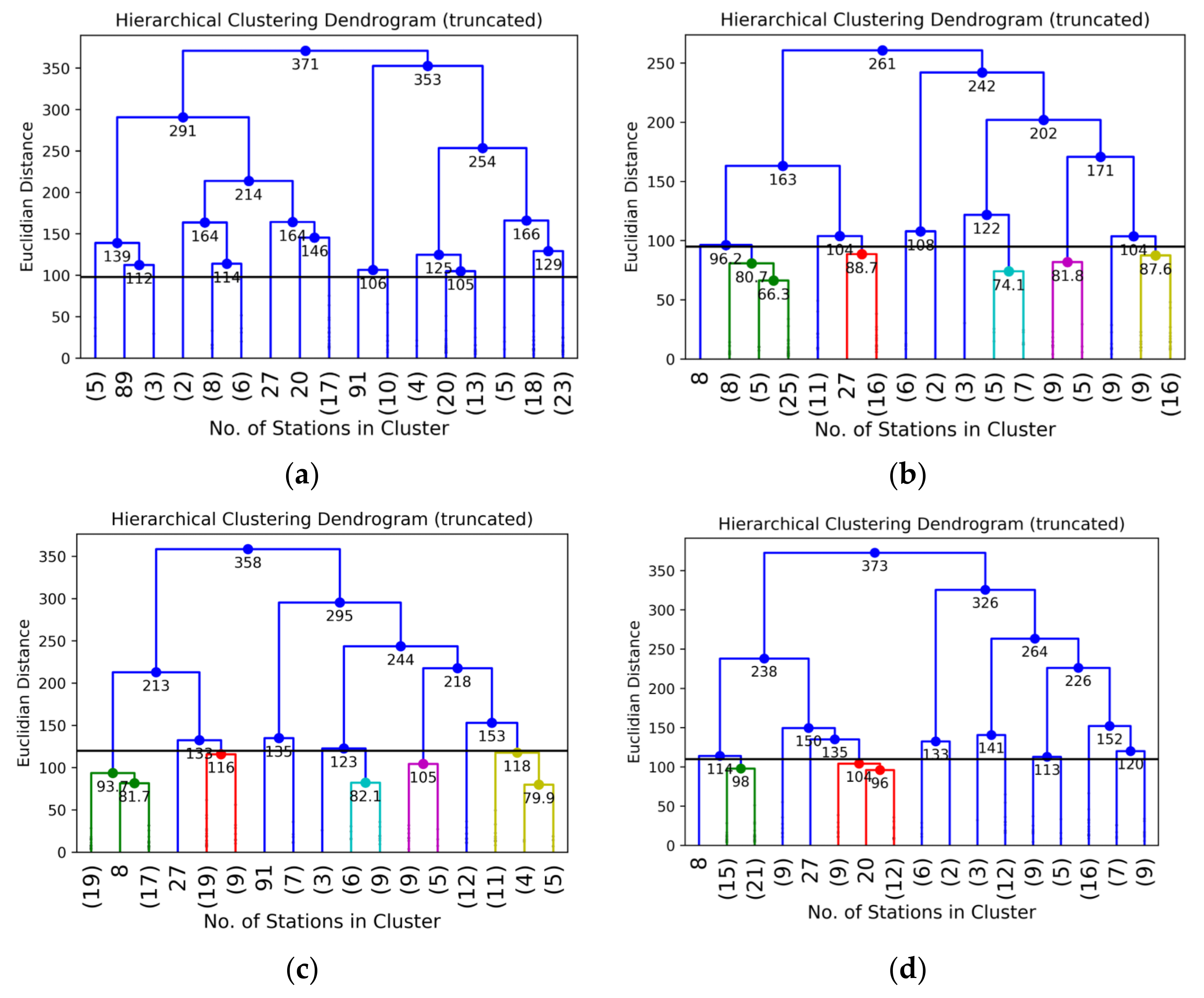
  • The climate signals in the form of component scores were obtained for the PCs, which cumulatively explained 90% of the data variance. These component scores were then used in the Agglomerative Hierarchical clustering (AHC) of the GCM. AHC would result in the clusters of GCMs having similar descriptive statistics. Through this step, we were able to identify the clusters or groups of GCMs having similar climate signals. The method has been described in Section 3.1.2; the clustering of GCMs has been illustrated with the help of a dendrogram tree of GCMs shown in Figure 3e for the climate zone 9 of the cold dry season. The optimum number of clusters is based upon the Euclidian distance [59] between the clusters. The dendrogram tree presents the meaningful information of different clusters and the Euclidian distances between the clusters.
  • The optimum number of clusters was determined with the help of a cluster validity index called the silhouette score (described in Section 3.1.5). The silhouette scores for different numbers of clusters have been shown in Table 1 for the climate zone 9 of the cold dry season. Two clusters are optimum for this case, as they produce the highest silhouette score. Euclidian distance of 120 has been evaluated, corresponding to the optimum number of clusters. The dendrogram tree was then truncated at a value of 120 Euclidian distance, as shown in Figure 3e, to obtain the number and identity of GCMs in each cluster.
GCMs presenting the extreme climate signals, in the form of a component score, were selected in each cluster in each climate zone [18].
Figure 4 illustrates the two clusters of GCMs for climate zone 9 of the cold dry season. Cluster 1 has 19 GCMs as shown in Figure 4a, and Cluster 2 has 2 GCMs as shown in Figure 4b. MIROC5 and MIROC-ESM are selected in cluster 1 and CNRM5 is selected in cluster 2, as they are presenting the extreme climate signals in the form of component scores.

3.3. Combining GCMs and Data Sampling

Multimodel combination is a practical methodology, which is employed by the climate research community to incorporate all the model outputs (historical or projections) for the climate impact modeling to reduce the uncertainty that may originate by the use of a single model [17,64]. The approaches which are generally used to combine the models are equally weighted mean and optimum weighted mean [65], and median. In this study, two methods have been used for combining the data of the selected GCMs at each zone. The one is taking the mean and the second is the median of the data of the selected GCMs in a climate zone.

3.4. Climate Change Trends Projections

Mann–Kendall (MK) test was used to detect the trend of the precipitation change in the study for the four seasons for the century. The study period has been divided into three parts to visualize the results every three decades. The magnitudes of the trends were determined through Sen’s slope. MK Test and Sen’s slope test have been described as follows.

3.4.1. Mann-Kendall Test (MK Test)

The MK test [66] is used to statistically detect monotonic increasing or decreasing trends. In this study, the MK test has been used to detect the seasonal precipitation trend for the projected period to detect statistically significant trends in the chronological precipitation data. In this non-parametric distribution test, “No trend” is assumed in the Null Hypothesis (Ho) and vice versa. Equations (3)–(5) are used to calculate the test statistics Z. Equation (6) presents the test statistics.
T = i = 1 n 1 j = i + 1 n s i g D j D i
s g n D j D i = + 1 i f   D j D i > 0 0 i f   D j D i = 0   1 i f   D j D i < 0
σ T = 1 18 n n 1 2 n + 5 p = 1 q t p t p 1 2 t p + 5
Z = T 1 σ   T i f   T > 0 0 i f   T = 0 T 1 σ   T i f   T < 0
where Di and Dj are the ith and jth observations in the time series in chronological order; the length of data is n; tp is the total number of data points in pth tied group, and the total number of tied groups is q; σ represents the variance. The negative Z value denotes the downward trend and vice versa. The Null Hypothesis of “No trend” is rejected, Z   >   Z 1 α / 2 indicates a statistically significant trend. The critical value Z 1 α / 2 corresponds to p-value 0.05. This trend has been detected at 138 stations in a region for each scenario.

3.4.2. Sen’s Slope Evaluation

The magnitude/slopes of the trends in the data were obtained using Sen’s method [67]. Sen’s slope is the median value in the set of linear slopes in the data. Sen’s slope is estimated through the following Equation (7).
T i = D j D k j k   for   ( 1     i   <   j     n ) ,
where the slope is denoted by Ti, Dj and Dk are the values at time steps j and k, respectively, and n is the total number of the data points number.

4. Results and Discussion

This section presents the results of each step of the study methodology. Section 4.1 shows the results of GCM selection. In Section 4.2, the significance of precipitation trends and magnitude are presented.

4.1. Formation of Climate Zones

The two major steps involved in the regionalization of the study are (1) Principal Component analysis and (2) Agglomerative Hierarchical Clustering. Climate change patterns have been visualized through the application of PCA on the historical daily precipitation data (1971–2005) of 138 stations for every season. Then the clusters of sites/stations presenting similar climate signals were identified through agglomerative hierarchical clustering, the results of each step of the clustering procedure are presented as follows.

4.1.1. Principal Component Analysis (PCA)

After execution, 20 significant principal components were identified which explained the cumulative variance of 95% of the data for each season in the study area. The cumulative variance by five, ten, fifteen, and twenty principal components have been shown in Table 2. According to these plots, approximately the first 20 PCs explained 94–95% of the variance in every season. These 20 PCs were engaged for the agglomerative cluster analysis in the next step of regionalization. The component scores were obtained for each PC at every station. These component scores represent the climate signals generated at the respective station. The climate signals of the first two leading principal components in the study area have been visualized for each season in Figure 5.
In the warm wet season, the first two principal components explained a cumulative variance of 44.8%. In cold dry, cold wet, and warm dry seasons, the cumulative variance of 41.2%, 45.7%, and 41.5%, respectively, were explained. The higher negative or positive signals/component scores correspond to high variability in the precipitation data and the lower signals depict the low variability. The percentage variance explained by each PC in different seasons has been mentioned in each panel of Figure 5. In the southwest of the region, the high negative climate signals were obtained in the cold wet and warm dry season but low negative signals were obtained in the warm wet and cold dry season, for the first principal component. For the second principal component, low negative component scores were obtained in all the seasons in the southwest of the region. In the north, according to the first Principal component, the positive medium to high component scores were obtained in cold dry, cold wet, and warm dry season, and negative high component scores were obtained in the warm wet season. Low negative climate signals in the northern region were obtained in all the seasons for the second-highest leading Principal Component. In the southeast of the region, highest spatial heterogeneity in climate signals has been observed, as positive highest component scores were obtained for the warm wet, cold wet, and warm dry season in the second principal component. The heterogeneity of the component scores, depicting the variability of the climate in the region, forms the basis of the clustering of the sites.

4.1.2. Agglomerative Hierarchical Clustering (AHC)

The clustering of the component scores of 138 stations for the first 20 leading PCs was done using Agglomerative Hierarchical Clustering. The number of optimum clusters was determined through a cluster validity test of silhouette score. The optimum clustering based on the silhouette score is decided corresponding to the highest score. The test suggested that the climate signals corresponding to the stations be optimally clustered into 17, 11, 10, and 14 for the warm wet, cold dry, cold wet seasons, and warm dry, respectively.
The maximum Euclidian distances were determined as 98, 95, 120, and 110, corresponding to the optimal number of clusters of 17, 11, 10, 14 for warm wet, cold dry, cold wet, and warm dry seasons, respectively. The dendrogram trees, as shown in Figure 6, were obtained through AHC. These trees were truncated at maximum Euclidian distances of 98, 95, 120, and 110 to obtain the optimum number of clusters and the station points in every cluster. The truncation bar in each season is also shown in Figure 6.

4.1.3. Climate Zones and Reference Site

All the clusters of stations were plotted on the map of the study area. Each cluster of stations having a homogeneous climate has been given a different color to differentiate them. For clear presentation, the cluster boundaries are made to demarcate the region into several climate zones. The transformation of the clusters of stations to the climate zones for each season has been presented in Figure 7.
After merging the outliers with the nearest clusters, the river basins are apportioned into 12, 9, 9, and 10 clusters for the warm wet, cold dry, cold wet, and warm dry seasons, respectively. The sites/station, which represented approximately the average of the climate signals of the stations in the cluster, has been termed as a reference station. These reference stations were identified in every cluster/climate zone of all the seasons.

4.2. GCM Selection

The GCMs were selected in every climate zone in every season based on the envelope-based approach. For the study area, selected GCMs using base period data (1971–2004) and projected data of RCP 4.5 and RCP 8.5 of 21 GCMs in different climate zones and seasons have been presented in Tables S2 and S3, respectively (in Supplementary Materials).

4.3. Seasonal Precipitation Trend Projection

Although some studies have evaluated climatic variability and its implications on the hydrological regime of the Jhelum and Chenab River basins, there is no clear agreement among them regarding climate change trends projections and their effects on the hydrological regime, specifically for the next century [16,68,69,70].
The seasonal trends of precipitation were evaluated for the projected data for two forcing scenarios of RCP 4.5 and RCP 8.5 and two combinations (mean and median) of the Ensemble members’ data. The trends and slopes have been assessed for consecutive three decadal projected periods, i.e., 2005–2040, 2041–2070, and 2071–2099 as well as the whole projected period of 2005–2099. The results show that the trends were statistically non-significant in most of the parts of the study area when the analyses were performed for the 3-decadal period. Whereas the trends were significant when the whole projected period was used in the analyses. Figure 8 and Figure 9 present the trend analyses for the period 2005–2099 for the two ensemble combination of MME-mean and MME-median, respectively.
The spatial distributions of the significance of the trends and the slopes have been presented in Figures S1–S4 (in Supplementary Materials). MK Test p-value has been mapped spatially for a region, and the green shades depict that the trend is significant for α ≤ 0.05. When the p-value is greater than 0.05, the trend is non-significant. p-value equals unity, and depicts no trend.

4.3.1. For 2005–2040

The data for the scenarios MME-mean and median of RCP 4.5, projected the significant increasing trends of 5–6 mm/year and 4–5 mm/year, respectively, in the warm dry season in the central part of the study area. For MME mean and median RCP 8.5, some traces of significant trends have been observed in the central part for cold dry season with magnitude ranges from 4 to 5 mm/year and 2 to 3 mm/year, respectively. In the north of the area, the data of MME-mean RCP 8.5 have projected significant positive trends of range 4–5 mm/year in east of the area.

4.3.2. For 2041–2070

The data of MME-mean RCP 8.5 have projected traces of significant decreasing trends in the warm wet season of magnitude ranging from 3 to 5 mm/year in the central part and positive significant trends ranging from 5 to 6 mm/year in the cold dry season in east. Some traces of increasing trends of magnitude 5–6 mm/year have been projected in the east of the study area for the cold dry season.
The data of MME-median RCP 8.5 have projected decreasing trends of 1–2 mm/year in east of the area for the cold dry season and increasing trends of 5–6 mm/year in the southwest for the warm dry season.

4.3.3. For 2071–2099

MME-mean and median RCP 4.5 have projected increasing trends for the warm dry season in the southeast and cold dry season in the west, respectively, with magnitude varies from 2–3 mm/year.

4.3.4. For 2005–2099

For MME-mean RCP 4.5 (refer to Figure 8), the significant decreasing trends have been projected in the whole study area for the warm wet season with magnitude varying between 1.85 and 4.9 mm/year in the central and north, 0.6–1.2 mm/year in southeast and southwest. In the cold dry season, the significant increasing trends range between 0.04 and 1.2 mm/year have been projected in central, north, east, and southeast. In the cold wet season, significant increasing trends have been projected in the north of the region with magnitude varying between 0.8 and 1.22 mm/year. Significant increasing trends have been noticed in warm dry in nearly all parts of the area except north, with magnitude varies between 0.81 and 3.27 mm/year.
For MME-mean RCP 8.5, significant increasing trends have been projected in the study area for cold dry and warm dry seasons with magnitude varying between 0.2 and 1.2 mm/year and 0.5–3.27 mm/year, respectively. Significant increasing trends have been projected in the north and southeast for the cold wet season with magnitudes varying between 0.5 and 1.63 mm/year.
For MME-median RCP 4.5 (refer to Figure 9), significant decreasing trends have been projected in the warm wet season in the north and central parts with magnitudes varying between 1.23 and 2.47 mm/year. For the cold dry season, significant positive trends have been projected in the east with magnitude ranges between 0.81 and 1.22 mm/year. Significant positive trends have been projected in nearly all of the study areas for the warm dry season with a magnitude that varies between 0.5 and 1.63 mm/year.
For MME-median RCP 8.5, significant increasing trends have been projected in cold dry in north and east and warm dry season in nearly all the area with magnitude varying between 0.5 and 1.22 mm/year.

5. Conclusions

There is currently no consensus on widely agreed criteria and approaches for GCM selection in previous research [71,72]. Studies continue to explore ways, be it statistical or dynamic, to minimize the uncertainty in the climate change projections [25]. To minimize uncertainty associated with the GCMs suitability across various regions with heterogeneous climates, this research proposed a novel method for the selection of GCMs in homogeneous climate zones based on daily seasonal precipitation statistics. These statistics are reflected by the reanalysis gridded data series spanning throughout 1970–2005 for the Jhelum and Chenab River basins. The GCMs were selected by agglomerative hierarchical clustering of PCs obtained through the data spanning over the baseline period of 1970–2005 and the projected data for two forcing scenarios spanning between 2005 and 2099. The PCs represented the climate variability signals produced by various GCMs’ data in the specific climate zone. Agglomerative hierarchical clustering of these climate signals produced the clusters of GCMs having the homogeneous variability of climate signals. The GCMs, producing the extreme climate signals in every cluster, were selected for the specific climate zone and season, thus fulfilling the criteria of envelope-based selection.
We sampled the daily precipitation data for the projected period using the selected GCMs for the two radiative forcing scenarios of RCP 4.5 and 8.5 and combining the data as mean and the median at every grid point, to detect the trends in the precipitation variability, in the Jhelum and Chenab River basins for the period spanning 2005 to 2099.
The machine learning algorithms modules of the Scikit-learn library of Python were used to develop a program for GCM selection, Data sampling, and trend detection. The program can be used to augment the decision support system for water resource management, even with the data of the new versions of the GCMs. However, the assessment of the future projections derived from the GCMs outputs are based on the forcing scenarios, which are unknown in the future, thus are fundamentally uncertain. So, it is important to understand the uncertainty associated with the GCMs’ outputs to use such simulations for the climate change impact assessment [73,74,75,76]. The following conclusions can be drawn from the results presented in the study:
(1)
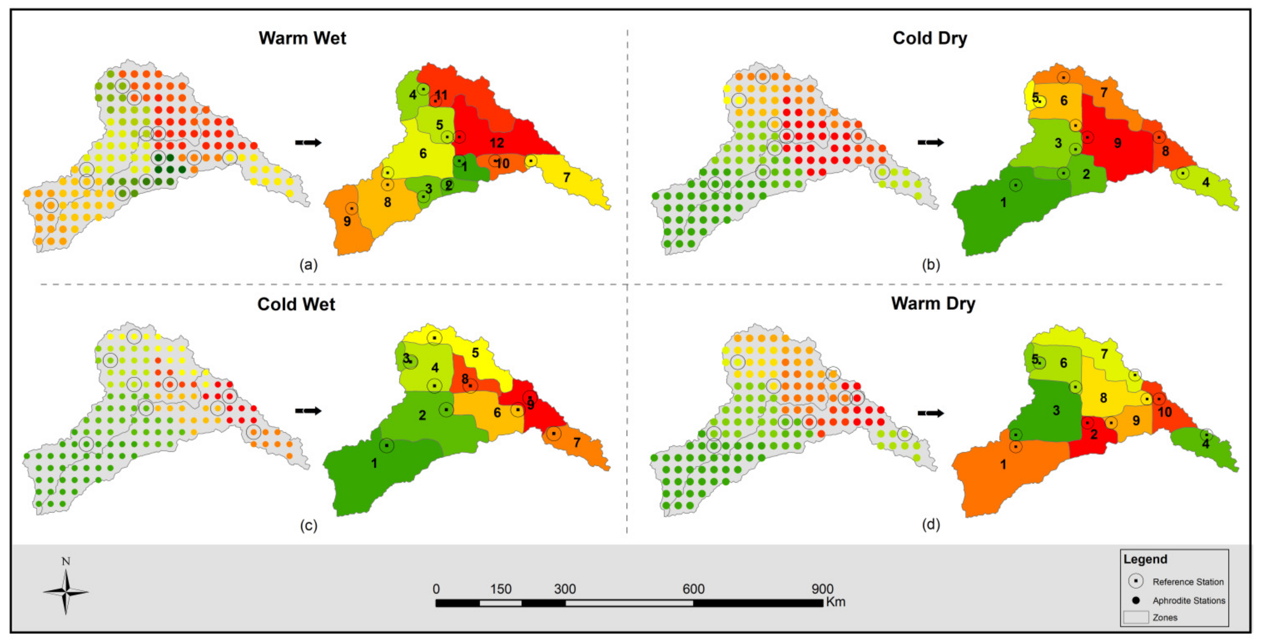
The high variability in the climate in Pakistan poses a major challenge to the scientific community to project the plausible trends in climate, specifically precipitation change, which is considered to be the basic representative of climate and covariates. It was intended to select the suitable GCMs across the multiple homogeneous climate zones, which are representative of spatiotemporal variability of the climate in a region. The conventional method of using the spatiotemporal area average [13,31,77] of the climate data or various spatial metrics after analyzing the individual grid point data [66,78,79] is very common among the climate research community. However, the selected GCMs, through these methods, may not represent variability and range of climate signals in the region having spatially heterogeneous climate statistics, which poses uncertainty in projecting the climate data using these GCMs. Therefore, the entire study area was divided into 12, 9, 9, and 10 homogeneous precipitation regions for the warm wet, cold dry, cold wet, and warm dry season, respectively. The selection of GCMs was made in each homogeneous climate zone.
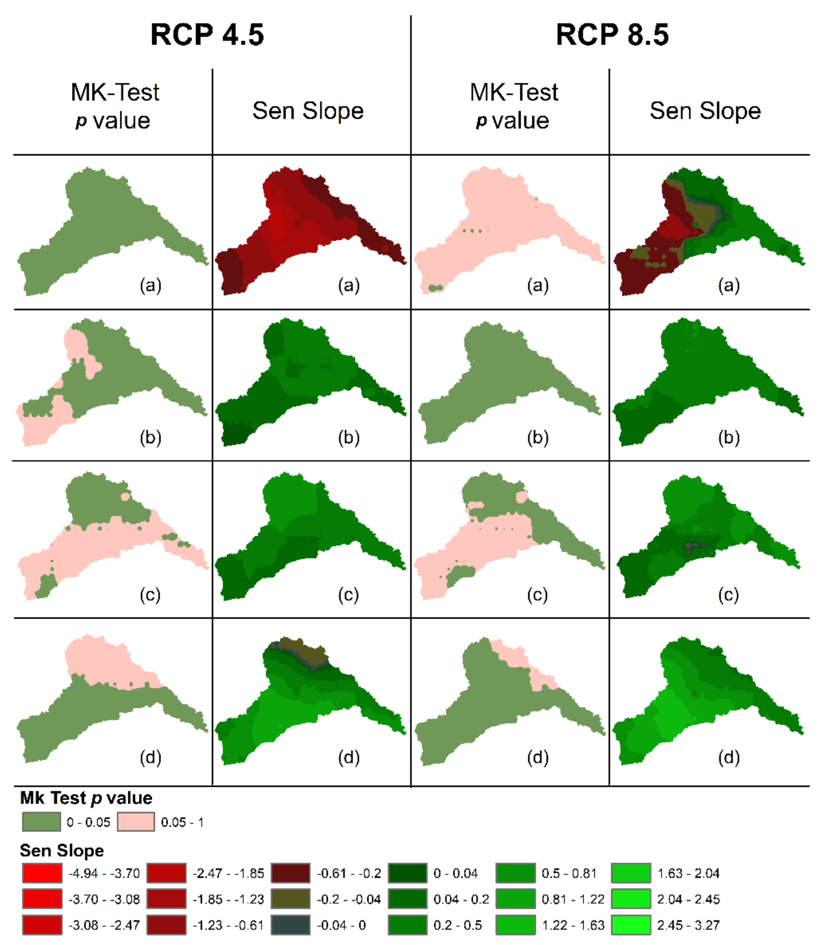
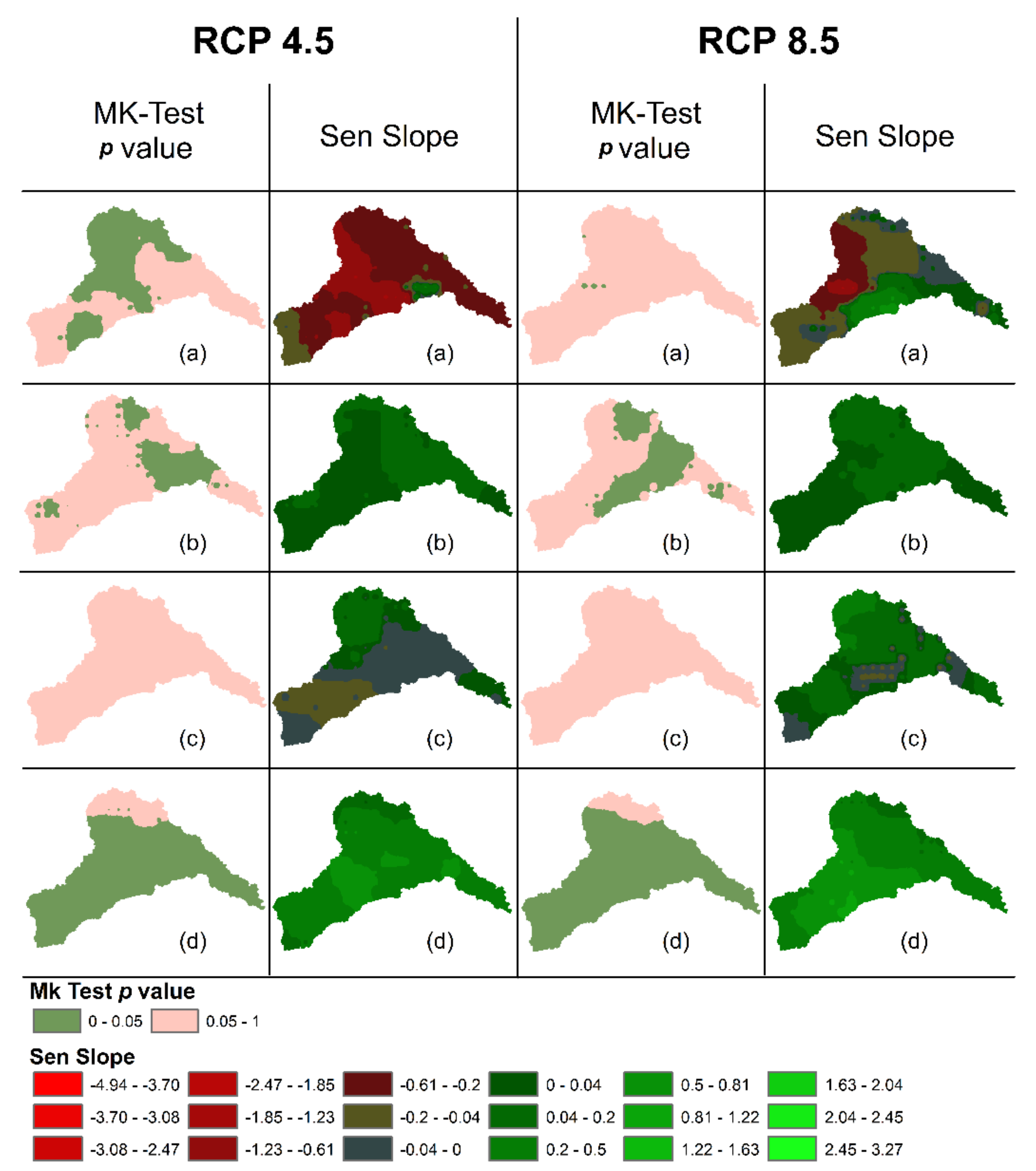
(2)
The precipitation trends were projected using the selected GCMs data on two forcing scenarios, RCP 4.5 and RCP 8.5, and two ensemble combinations; mean and median, thus making the total of four scenarios (RCP 4.5 Mean, RCP 4.5 Median, RCP 8.5 Mean, and RCP 8.5 Median). The trends projected using these scenarios provide the details of the range of trend variability of climate change in the region, with the knowledge of maximum increasing and decreasing trend quantification in the region seasonally, which is the purpose of envelope-based selection of GCMs.
Statistically significant trends were projected when the analyses were performed using the study period of 2005–2099. Significant negative trends were projected in the warm wet season and significant positive trends were projected in warm dry seasons for RCP 4.5. For RCP 8.5, statistically significant positive trends were projected in cold dry and warm dry seasons. The high evaporation and convection rate over the agro-economic zones is anticipated to be the cause of increasing trends in high emission scenarios.
Further research avenues that can be explored include a redefinition of the homogeneous climate zones based on GCMs’ output and selection of GCMs based on spatial coherence of these climate regions with the regions derived through observed or high-resolution reanalysis data.

Supplementary Materials

The following supporting information can be downloaded at: https://www.mdpi.com/article/10.3390/atmos13020190/s1. Table S1. Comparative analysis of APHRODITE and ERA5 monthly dataset. Pearson correlation coefficients and Kolmogorov Smirnov Test results (KS Test). (The shaded p-values are >0.05, depicting the null hypothesis of similar distribution, is not rejected). Table S2. Descriptions of the general circulation models (GCMs) used in the study. Table S2. Selected GCMs using RCP 4.5 and climate Zones for seasons warm wet cold dry cold wet and warm dry. Table S3: Selected GCMs using RCP 8.5 scenarios for seasons Warm Wet, Cold Dry, Cold Wet and Warm Dry. Figure S1. Mann Kendall trend detection and Sen’s slope results for MME-Mean using RCP 4.5 (a) Warm Wet (b) Cold Dry (c) Cold Wet (d) Warm Dry. Figure S2. Mann Kendall trend detection and Sen’s Slope results for MME-Median using RCP 4.5 (a) Warm Wet (b) Cold Dry (c) Cold Wet (d) Warm Dry. Figure S3. Mann Kendall trend detection and Sen’s slope results for MME-Mean using RCP 8.5 (a) Warm Wet (b) Cold Dry (c) Cold Wet (d) Warm Dry. Figure S4. Mann Kendall trend detection and Sen’s slope results for MME-Median using RCP 8.5 (a) Warm Wet (b) Cold Dry (c) Cold Wet (d) Warm Dry.

Author Contributions

Conceptualization: A.N. and H.U.R.; Data curation: U.e.H., S.A.J., J.A. and M.S., Formal analysis: A.N., S.H. and S.A.; Investigation: U.e.H., H.F.G. and A.N.; Methodology: S.A. and J.A.; Project administration: S.A. and H.U.R.; Software: S.A.J. and A.N.; Supervision: H.F.G.; Validation: A.N. and H.U.R.; Visualization: S.A.J., A.N.; Writing—S.H., S.A. and H.F.G. All authors have read and agreed to the published version of the manuscript.

Funding

This research received no external funding.

Data Availability Statement

The data presented in this study are openly available in [GitHub—SaadAhmedJamal/PlausiblePrecipitationTrends: for jehlum and chenab basin https://github.com/SaadAhmedJamal/PlausiblePrecipitationTrends, accessed on 2 November 2021].

Acknowledgments

The authors highly acknowledge the resources and facilities provided by NUST Institute of Civil Engineering for the successful compliance of the present study.

Conflicts of Interest

The authors declare no conflict of interest.

References

  1. Shah, S.M.H.; Mustaffa, Z.; Teo, F.Y.; Imam, M.A.H.; Yusof, K.W.; Al-Qadami, E.H.H. A review of the flood hazard and risk management in the South Asian Region, particularly Pakistan. Sci. Afr. 2020, 10, e00651. [Google Scholar] [CrossRef]
  2. Tariq, M.A.U.R.; Van De Giesen, N. Floods and flood management in Pakistan. Phys. Chem. Earth Parts A/B/C 2012, 47, 11–20. [Google Scholar] [CrossRef]
  3. Ahmed, K.; Shahid, S.; Chung, E.-S.; Wang, X.; Harun, S.B. Climate Change Uncertainties in Seasonal Drought Severity-Area-Frequency Curves: Case of Arid Region of Pakistan. J. Hydrol. 2019, 570, 473–485. [Google Scholar] [CrossRef]
  4. Anjum, M.N.; Ding, Y.J.; Shangguan, D.H. Simulation of the projected climate change impacts on the river flow regimes under CMIP5 RCP scenarios in the westerlies dominated belt, northern Pakistan. Atmos. Res. 2019, 227, 233–248. [Google Scholar] [CrossRef]
  5. Bosshard, T.; Carambia, M.; Goergen, K.; Kotlarski, S.; Krahe, P.; Zappa, M.; Schär, C. Quantifying uncertainty sources in an ensemble of hydrological climate-impact projections. Water Resour. Res. 2013, 49, 1523–1536. [Google Scholar] [CrossRef] [Green Version]
  6. Sood, A.; Smakhtin, V. Global hydrological models: A review. Hydrol. Sci. J. 2015, 60, 549–565. [Google Scholar] [CrossRef]
  7. Pradhan, P.; Shrestha, S.; Sundaram, S.M.; Virdis, S.G.P. Evaluation of the CMIP5 general circulation models for simulating the precipitation and temperature of the Koshi River Basin in Nepal. J. Water Clim. Chang. 2021, 12, 3282–3296. [Google Scholar] [CrossRef]
  8. Almazroui, M.; Islam, M.N.; Saeed, F.; Saeed, S.; Ismail, M.; Ehsan, M.A.; Diallo, I.; O’Brien, E.; Ashfaq, M.; Martínez-Castro, D.; et al. Projected Changes in Temperature and Precipitation Over the United States, Central America, and the Caribbean in CMIP6 GCMs. Earth Syst. Environ. 2021, 5, 1–24. [Google Scholar] [CrossRef]
  9. Jang, D. An Application of ANN Ensemble for Estimating of Precipitation Using Regional Climate Models. Adv. Civ. Eng. 2021, 2021, 7363471. [Google Scholar] [CrossRef]
  10. Shiru, M.S.; Chung, E.-S. Performance evaluation of CMIP6 global climate models for selecting models for climate projection over Nigeria. Theor. Appl. Climatol. 2021, 146, 599–615. [Google Scholar] [CrossRef]
  11. Chen, J.; Brissette, F.P.; Poulin, A.; Leconte, R. Overall uncertainty study of the hydrological impacts of climate change for a Canadian watershed. Water Resour. Res. 2011, 47. [Google Scholar] [CrossRef]
  12. IPCC. IPCC Expert Meeting on Emission Scenarios; IPCC: Washington, DC, USA, 2005. [Google Scholar]
  13. Lutz, A.F.; ter Maat, H.W.; Biemans, H.; Shrestha, A.B.; Wester, P.; Immerzeel, W.W. Selecting Representative Climate Models for Climate Change Impact Studies: An Advanced Envelope-Based Selection Approach. Int. J. Climatol. 2016, 36, 3988–4005. [Google Scholar] [CrossRef] [Green Version]
  14. Mendlik, T.; Gobiet, A. Selecting Climate Simulations for Impact Studies Based on Multivariate Patterns of Climate Change. Clim. Chang. 2016, 135, 381–393. [Google Scholar] [CrossRef] [PubMed] [Green Version]
  15. Chhin, R.; Yoden, S. Ranking CMIP5 GCMs for Model Ensemble Selection on Regional Scale: Case Study of the Indochina Region. J. Geophys. Res. Atmos. 2018, 123, 8949–8974. [Google Scholar] [CrossRef]
  16. Azmat, M.; Qamar, M.U.; Huggel, C.; Hussain, E. Future Climate and Cryosphere Impacts on the Hydrology of a Scarcely Gauged Catchment on the Jhelum River Basin, Northern Pakistan. Sci. Total Environ. 2018, 639, 961–976. [Google Scholar] [CrossRef]
  17. Weigel, A.P.; Knutti, R.; Liniger, M.A.; Appenzeller, C. Risks of Model Weighting in Multimodel Climate Projections. J. Clim. 2010, 23, 4175–4191. [Google Scholar] [CrossRef]
  18. Knutti, R.; Furrer, R.; Tebaldi, C.; Cermak, J.; Meehl, G. Challenges in Combining Projections from Multiple Climate Models. J. Clim. 2010, 23, 2739–2758. [Google Scholar] [CrossRef] [Green Version]
  19. McSweeney, C.F.; Jones, R.G.; Lee, R.W.; Rowell, D.P. Selecting CMIP5 GCMs for downscaling over multiple regions. Clim. Dyn. 2015, 44, 3237–3260. [Google Scholar] [CrossRef] [Green Version]
  20. Zhang, H.; Huang, G.H.; Wang, D.; Zhang, X. Uncertainty assessment of climate change impacts on the hydrology of small prairie wetlands. J. Hydrol. 2011, 396, 94–103. [Google Scholar] [CrossRef] [Green Version]
  21. Cannon, A.J. Selecting GCM Scenarios that Span the Range of Changes in a Multimodel Ensemble: Application to CMIP5 Climate Extremes Indices. J. Clim. 2015, 28, 1260–1267. [Google Scholar] [CrossRef]
  22. Carter, T.R. General Guidelines on the Use of Scenario Data for Climate Impact and Adaptation Assessment, 2nd ed.; Task Group on Data and Scenario Support for Impact and Climate Assessment (TGICA); Intergovernmental Panel on Climate Change (IPCC): Helsinki, Finland, 2007; p. 66. [Google Scholar]
  23. Pennell, C.; Reichler, T. On the Effective Number of Climate Models. J. Clim. 2011, 24, 2358–2367. [Google Scholar] [CrossRef]
  24. Masson, D.; Knutti, R. Climate model genealogy. Geophys. Res. Lett. 2011, 38, 1–4. [Google Scholar] [CrossRef]
  25. Nusrat, A.; Gabriel, H.F.; Haider, S.; Ahmad, S.; Shahid, M.; Ahmed Jamal, S. Application of Machine Learning Techniques to Delineate Homogeneous Climate Zones in River Basins of Pakistan for Hydro-Climatic Change Impact Studies. Appl. Sci. 2020, 10, 6878. [Google Scholar] [CrossRef]
  26. Khan, F.; Pilz, J.; Ali, S. Evaluation of CMIP5 models and ensemble climate projections using a Bayesian approach: A case study of the Upper Indus Basin, Pakistan. Environ. Ecol. Stat. 2021, 28, 383–404. [Google Scholar] [CrossRef]
  27. Yaseen, M.; Ahmad, I.; Guo, J.L.; Azam, M.I.; Latif, Y. Spatiotemporal Variability in the Hydrometeorological Time-Series over Upper Indus River Basin of Pakistan. Adv. Meteorol. 2020, 2020. [Google Scholar] [CrossRef]
  28. Asmat, U.; Athar, H.; Nabeel, A.; Latif, M. An AOGCM based assessment of interseasonal variability in Pakistan. Clim. Dyn. 2018, 50, 349–373. [Google Scholar] [CrossRef]
  29. Azmat, M.; Wahab, A.; Huggel, C.; Qamar, M.U.; Hussain, E.; Ahmad, S.; Waheed, A. Climatic and hydrological projections to changing climate under CORDEX-South Asia experiments over the Karakoram-Hindukush-Himalayan water towers. Sci. Total Environ. 2020, 703, 135010. [Google Scholar] [CrossRef]
  30. Ahmad, M.; Chand, S.; Yaseen, M. High resolution bayesian spatio-temporal precipitation modelling in pakistan for the appraisal of trends. Pak. J. Agric. Sci. 2020, 57, 1669–1680. [Google Scholar] [CrossRef]
  31. Mahmood, R.; Jia, S.; Tripathi, N.K.; Shrestha, S. Precipitation Extended Linear Scaling Method for Correcting GCM Precipitation and Its Evaluation and Implication in the Transboundary Jhelum River Basin. Atmosphere 2018, 9, 160. [Google Scholar] [CrossRef] [Green Version]
  32. Ateequr, R.; Ghumman, A.R.; Ahmad, S.; Hashmi, H.N. Performance assessment of artificial neural networks and support vector regression models for stream flow predictions. Environ. Monit. Assess. 2018, 190. [Google Scholar] [CrossRef]
  33. Lenderink, G.; van Ulden, A.; van den Hurk, B.; Keller, F. A study on combining global and regional climate model results for generating climate scenarios of temperature and precipitation for the Netherlands. Clim. Dyn. 2007, 29, 157–176. [Google Scholar] [CrossRef] [Green Version]
  34. Wang, B. The Asian Monsoon; Springer Science & Business Media: Cham, Switzerland, 2006. [Google Scholar]
  35. Dimri, A.; Niyogi, D.; Barros, A.; Ridley, J.; Mohanty, U.; Yasunari, T.; Sikka, D. Western disturbances: A review. Rev. Geophys. 2015, 53, 225–246. [Google Scholar] [CrossRef]
  36. Khatri, W.D.; Xiefei, Z.; Ling, Z. Interannual and Interdecadal Variations in Tropical Cyclone Activity over the Arabian Sea and the Impacts over Pakistan. In High-Impact Weather Events over the SAARC Region; Springer: Berlin/Heidelberg, Germany, 2015; pp. 129–145. [Google Scholar]
  37. Rasul, G.; Chaudhry, Q. Review of advance in research on Asian summer monsoon. Pak. J. Meteorol. 2010, 6, 1–10. [Google Scholar]
  38. Parvaze, S.; Ahmad, D. Meteorological Drought Quantification with Standardized Precipitation Index for Jhelum Basin in Kashmir Valley. Int. J. Adv. Res. Comput. Sci. Manag. 2018, 7, 688–697. [Google Scholar]
  39. Mahmood, R.; Babel, M.S.; Jia, S. Assessment of temporal and spatial changes of future climate in the Jhelum river basin, Pakistan and India. Weather Clim. Extrem. 2015, 10, 40–55. [Google Scholar] [CrossRef] [Green Version]
  40. Rizwan, M.; Jamal, K.; Chen, Y.; Chauhdary, J.N.; Zheng, D.; Anjum, L.; Youhua, R.; Pan, X. Precipitation Variations under a Changing Climate from 1961-2015 in the Source Region of the Indus River. Water 2019, 11, 1366. [Google Scholar] [CrossRef] [Green Version]
  41. Immerzeel, W.W.; Wanders, N.; Lutz, A.F.; Shea, J.M.; Bierkens, M.F.P. Reconciling High-Altitude Precipitation in the Upper Indus Basin with Glacier Mass Balances and Runoff. Hydrol. Earth Syst. Sci. 2015, 19, 4673–4687. [Google Scholar] [CrossRef] [Green Version]
  42. Lutz, A.; Immerzeel, W.; Kraaijienbrink, P.D.A. Gridded Meteorological Datasets and Hydrological Modelling in the Upper Indus Basin; Future Water: Wageningen, The Netherlands, 2014; p. 83. [Google Scholar]
  43. Yatagai, A.; Kamiguchi, K.; Arakawa, O.; Hamada, A.; Yasutomi, N.; Kitoh, A. APHRODITE: Constructing a Long-Term Daily Gridded Precipitation Dataset for Asia Based on a Dense Network of Rain Gauges. Bull. Am. Meteor. Soc. 2012, 93, 1401–1415. [Google Scholar] [CrossRef]
  44. Lutz, A.; Immerzeel, W. Water Availability Analysis for the Upper Indus, Ganges and Brahmaputra River Basins; Future Water: Wageningen, The Netherlands, 2013; p. 85. [Google Scholar]
  45. Hersbach, H.; Bell, B.; Berrisford, P.; Biavati, G.; Horányi, A.; Muñoz Sabater, J.; Nicolas, J.; Peubey, C.; Radu, R.; Rozum, I.; et al. ERA5 Hourly Data on Single Levels from 1979 to Present. Available online: https://cds.climate.copernicus.eu/cdsapp#!/dataset/reanalysis-era5-single-levels?tab=form (accessed on 2 November 2021).
  46. Department of Civil and Environmental Engineering Princeton University. Global Meteorological Forcing Dataset for Land Surface Modeling; Computational and Information Systems Laboratory, Research Data Archive at the National Center for Atmospheric Research: Boulder, CO, USA, 2006. [Google Scholar] [CrossRef]
  47. Chen, H.-P.; Sun, J.-Q.; Li, H.-X. Future changes in precipitation extremes over China using the NEX-GDDP high-resolution daily downscaled data-set. Atmos. Ocean. Sci. Lett. 2017, 10, 403–410. [Google Scholar] [CrossRef] [Green Version]
  48. Kumar, P.; Kumar, S.; Barat, A.; Sarthi, P.P.; Sinha, A.K. Evaluation of NASA’s NEX-GDDP-simulated summer monsoon rainfall over homogeneous monsoon regions of India. Theor. Appl. Climatol. 2020, 141, 525–536. [Google Scholar] [CrossRef]
  49. Taylor, E.K.; Ronald, S.; Meehl, G. An Overview of CMIP5 and the Experiment Design. Bull. Am. Meteor. Soc. 2011, 93, 485–498. [Google Scholar] [CrossRef] [Green Version]
  50. Pedregosa, F.; Varoquaux, G.; Gramfort, A.; Michel, V.; Thirion, B.; Grisel, O.; Blondel, M.; Prettenhofer, P.; Weiss, R.; Dubourg, V.; et al. Scikit-learn: Machine Learning in Python. J. Mach. Learn. Res. 2011, 12, 2825–2830. [Google Scholar]
  51. Asong, Z.E.; Khaliq, M.N.; Wheater, H.S. Regionalization of Precipitation Characteristics in the Canadian Prairie Provinces Using Large-scale Atmospheric Covariates and Geophysical Attributes. Stoch. Environ. Res. Risk Assess. 2015, 29, 875–892. [Google Scholar] [CrossRef]
  52. Liu, M.; Huang, Y.; Li, Z.; Tong, B.; Liu, Z.; Sun, M.; Jiang, F.; Zhang, H. The Applicability of LSTM-KNN Model for Real-Time Flood Forecasting in Different Climate Zones in China. Water 2020, 12, 440. [Google Scholar] [CrossRef] [Green Version]
  53. Zeraatpisheh, M.; Bakhshandeh, E.; Emadi, M.; Li, T.; Xu, M. Integration of PCA and Fuzzy Clustering for Delineation of Soil Management Zones and Cost-Efficiency Analysis in a Citrus Plantation. Sustainability 2020, 12, 5809. [Google Scholar] [CrossRef]
  54. Chen, Y.; Zheng, B.; Hu, Y. Mapping Local Climate Zones Using ArcGIS-Based Method and Exploring Land Surface Temperature Characteristics in Chenzhou, China. Sustainability 2020, 12, 2974. [Google Scholar] [CrossRef] [Green Version]
  55. Benestad, R.E.; Chen, D.; Mezghani, A.; Fan, L.; Parding, K. On Using Principal Components to Represent Stations in Empirical–Statistical Downscaling. Tellus A 2015, 67, 28326. [Google Scholar] [CrossRef]
  56. Liu, Q.; Huang, C.; Li, H. Quality Assessment by Region and Land Cover of Sharpening Approaches Applied to GF-2 Imagery. Appl. Sci. 2020, 10, 3673. [Google Scholar] [CrossRef]
  57. Abbasi, F.; Bazgeer, S.; Kalehbasti, P.R.; Oskoue, E.A.; Haghighat, M.; Kalebasti, P.R. New climatic zones in Iran: A comparative study of different empirical methods and clustering technique. Theor. Appl. Climatol. 2021, 147, 47–61. [Google Scholar] [CrossRef]
  58. Sammour, M.; Othman, Z.A.; Muda, Z.; Ibrahim, R. An agglomerative hierarchical clustering with association rules for discovering climate change patterns. Int. J. Adv. Comput. Sci. Appl. 2019, 10, 233–240. [Google Scholar] [CrossRef]
  59. Mimmack, G.M.; Mason, S.J.; Galpin, J.S. Choice of Distance Matrices in Cluster Analysis: Defining Regions. J. Clim. 2001, 14, 2790–2797. [Google Scholar] [CrossRef]
  60. Nam, W.; Shin, H.; Jung, Y.; Joo, K.; Heo, J.-H. Delineation of the Climatic Rainfall Regions of South Korea Based on a Multivariate Analysis and Regional Rainfall Frequency Analyses. Int. J. Climatol. 2015, 35, 777–793. [Google Scholar] [CrossRef]
  61. Carvalho, M.J.; Melo-Gonçalves, P.; Teixeira, J.C.; Rocha, A. Regionalization of Europe Based on a K-Means Cluster Analysis of the Climate Change of Temperatures and Precipitation. Phys. Chem. Earth Parts A/B/C 2016, 94, 22–28. [Google Scholar] [CrossRef] [Green Version]
  62. Rousseeuw, P.J. Silhouettes: A graphical aid to the interpretation and validation of cluster analysis. J. Comput. Appl. Math. 1987, 20, 53–65. [Google Scholar] [CrossRef] [Green Version]
  63. Van Vuuren, D.P.; Edmonds, J.; Kainuma, M.; Riahi, K.; Thomson, A.; Hibbard, K.; Hurtt, G.C.; Kram, T.; Krey, V.; Lamarque, J.-F.; et al. The Representative Concentration Pathways: An Overview. Clim. Change 2011, 109, 5–31. [Google Scholar] [CrossRef]
  64. Rozante, J.; Moreira, D.; Godoy, R.C.M.; Fernandes, A. Multi-model ensemble: Technique and validation. Geosci. Model Dev. Discuss. 2014, 7, 2933–2959. [Google Scholar] [CrossRef] [Green Version]
  65. Stephenson, D.B.; Coelho, C.A.S.; Doblas-Reyes, F.J.; Balmaseda, M. Forecast assimilation: A unified framework for the combination of multi-model weather and climate predictions. Tellus A Dyn. Meteorol. Oceanogr. 2005, 57, 253–264. [Google Scholar] [CrossRef]
  66. Salman, S.A.; Shahid, S.; Ismail, T.; Ahmed, K.; Wang, X.-J. Selection of Climate Models for Projection of Spatiotemporal Changes in Temperature of Iraq with Uncertainties. Atmos. Res. 2018, 213, 509–522. [Google Scholar] [CrossRef]
  67. Sen, P.K. Estimates of the Regression Coefficient Based on Kendall’s Tau. J. Am. Stat. Assoc. 1968, 63, 1379–1389. [Google Scholar] [CrossRef]
  68. Mahmood, R.; Jia, S.F. Spatial and temporal hydro-climatic trends in the transboundary Jhelum River basin. J. Water Clim. Change 2017, 8, 423–440. [Google Scholar] [CrossRef] [Green Version]
  69. Jasrotia, A.S.; Baru, D.; Kour, R.; Ahmad, S.; Kour, K. Hydrological modeling to simulate stream flow under changing climate conditions in Jhelum catchment, western Himalaya. J. Hydrol. 2021, 593. [Google Scholar] [CrossRef]
  70. Dahri, Z.H.; Ludwig, F.; Moors, E.; Ahmad, S.; Ahmad, B.; Ahmad, S.; Riaz, M.; Kabat, P. Climate change and hydrological regime of the high-altitude Indus basin under extreme climate scenarios. Sci. Total Environ. 2021, 768, 144467. [Google Scholar] [CrossRef] [PubMed]
  71. McMahon, T.A.; Peel, M.C.; Karoly, D.J. Assessment of Precipitation and Temperature Data from CMIP3 Global Climate Models for Hydrologic Simulation. Hydrol. Earth Syst. Sci. 2015, 19, 361–377. [Google Scholar] [CrossRef] [Green Version]
  72. Smith, I.; Chandler, E. Refining Rainfall Projections for the Murray Darling Basin of South-East Australia—The Effect of Sampling Model Results Based on Performance. Clim. Chang. 2010, 102, 377–393. [Google Scholar] [CrossRef]
  73. Xu, C.-y.; Widén, E.; Halldin, S. Modelling Hydrological Consequences of Climate Change—Progress and Challenges. Adv. Atmos. Sci. 2005, 22, 789–797. [Google Scholar] [CrossRef]
  74. Kay, A.L.; Davies, H.N.; Bell, V.A.; Jones, R.G. Comparison of Uncertainty Sources for Climate Change Impacts: Flood Frequency in England. Clim. Change 2009, 92, 41–63. [Google Scholar] [CrossRef]
  75. Woldemeskel, F.M.; Sharma, A.; Sivakumar, B.; Mehrotra, R. An Error Estimation Method for Precipitation and Temperature Projections for Future Climates. J. Geophys. Res. 2012, 117, D22. [Google Scholar] [CrossRef]
  76. Zhang, X.; Xu, Y.-P.; Fu, G. Uncertainties in SWAT Extreme Flow Simulation under Climate Change. J. Hydrol. 2014, 515, 205–222. [Google Scholar] [CrossRef]
  77. Latif, M.; Hannachi, A.; Syed, F.S. Analysis of Rainfall Trends over Indo-Pakistan Summer Monsoon and Related Dynamics Based on CMIP5 Climate Model Simulations. Int. J. Climatol. 2018, 38, e577–e595. [Google Scholar] [CrossRef]
  78. Srinivasa Raju, K.; Sonali, P.; Nagesh Kumar, D. Ranking of CMIP5-based global climate models for India using compromise programming. Theor. Appl. Climatol. 2017, 128, 563–574. [Google Scholar] [CrossRef]
  79. Khan, N.; Shahid, S.; Ahmed, K.; Ismail, T.; Nawaz, N.; Son, M. Performance Assessment of General Circulation Model in Simulating Daily Precipitation and Temperature Using Multiple Gridded Datasets. Water 2018, 10, 1793. [Google Scholar] [CrossRef] [Green Version]
Figure 1. Study Area Digital Elevation Model (DEM) also presents the observed gauging station and Grid stations in the study area.
Atmosphere 13 00190 g001
Figure 2. Methodology Flow Chart.
Atmosphere 13 00190 g002
Figure 3. Climate zones for the season cold dry and indication of the zone 9 which is considered for illustration (a) orientation of Zone 9 in study area (stations with similar climate have been given same colored marker in first map) (b) cumulative percentage of explained variance by each PCs (c) scatter plot of PC1 and PC2 (d) scree plot showing the percentage of explained variance by individual PCs (e) dendrogram tree with cut off bar in red.
Atmosphere 13 00190 g003
Figure 4. Agglomerative Hierarchical Clustering of GCMs at climate Zone 9 (a) cluster 1 with 19 GCMs and component scores (b) cluster 2 with 2 GCMs and respective component score.
Atmosphere 13 00190 g004
Figure 5. The spatial distribution of the component scores for the first two principal components (PC), percentage variance explained by the PCs are written in each panel (a) warm-wet (PC1), (b) cold dry (PC1), (c) cold wet (PC1), (d) warm dry (PC1), (e) warm wet (PC2), (f) cold dry (PC2), (g) cold wet (PC2) and (h) warm dry (PC2) seasons.
Atmosphere 13 00190 g005
Figure 6. Dendrogram trees presenting the number of stations in each cluster (in Bracket) and cut-off bars corresponding to the optimum Euclidean distance, based on the Silhouette Score for climate zoning for: (a) warm wet, (b) cold dry, (c) cold wet, and (d) warm dry seasons.
Atmosphere 13 00190 g006
Figure 7. The transition of clusters into Climate zones in the study area in the (a) warm wet, (b) cold dry, (c) cold wet, and (d) warm dry seasons.
Atmosphere 13 00190 g007
Figure 8. Mann Kendall trend detection and Sen’s slope results for MME-Mean using RCP 4.5 and RCP 8.5 for analysis period (2005–2099) (a) Warm Wet (b) Cold Dry (c) Cold Wet (d) Warm Dry.
Atmosphere 13 00190 g008
Figure 9. Mann Kendall trend detection and Sen’s slope results for MME-Median using RCP 4.5 and RCP 8.5 for analysis period (2005–2099) (a) Warm Wet (b) Cold Dry (c) Cold Wet (d) Warm Dry.
Atmosphere 13 00190 g009
Table 1. Silhouette score corresponding to the different number of clusters of GCMs at the reference station of Climate Zone 9 of Cold Dry Season. The highlighted cells are the optimum number of clusters and maximum Silhouette Score.
Number of ClustersSilhouette Score Number of ClustersSilhouette Score
20.027960.0056
30.024970.0028
40.018480.0033
50.017190.0032
Table 2. Cumulative percentage of explained variance of Principal Components.
Season5 PCs10 PCs15PCs 20 PCs
Warm Wet78889395
Cold Dry77879194
Cold Wet77889295
Warm Dry77869295
Publisher’s Note: MDPI stays neutral with regard to jurisdictional claims in published maps and institutional affiliations.

