Article

Extreme Low Flow Estimation under Climate Change

1
EDF/R&D 7 boulevard Gaspard Monge, 91120 Palaiseau, France
2
EDF/DTG, 134 rue de l’étang, 38950 Saint-Martin-le-Vinoux, France
*
Author to whom correspondence should be addressed.
Atmosphere 2022, 13(2), 164; https://doi.org/10.3390/atmos13020164
Submission received: 27 October 2021 / Revised: 11 January 2022 / Accepted: 15 January 2022 / Published: 20 January 2022
(This article belongs to the Special Issue Extreme Climate Events in France)

Abstract

:
Climate change’s impact on water availability has been widely studied, including its impact on very rare values quantified by return levels using the statistical extreme value theory. However, the application of this theory to estimate extreme low flows is barely justified due to a large temporal dependency and a physically highly bounded lower tail. One possible way of overcoming this difficulty is to simulate a very large sample of river flow time series consistent with the observations or the climate projections in order to enable empirical rare percentile estimations. In this paper, such an approach based on simulation is developed and tested for a small mountainous watershed in the French Alps. A bivariate generator of daily temperature and rainfall, developed in collaboration with Paris-Saclay University and based on hidden Markov models, is used to produce a large number of temperature and rainfall time series, further provided as input to a hydrological model to produce a similarly large sample of river flow time series. This sample is statistically analyzed in terms of low flow occurrence and intensity. This framework is adapted to the analysis of both current climate conditions and projected future climate. To study historical low flow situations, the bivariate temperature and rainfall model is fitted to the observed time series while bias-adjusted climate model outputs are used to calibrate the generator for the projections. The approach seems promising and could be further improved for use in more specific studies dedicated to the climate change impact on local low flow situations.

1. Introduction

The adaptation to climate change of hydropower or thermal power plants necessitates the identification and characterization of high impact hazards. Extremely low river flow is one of these situations. Climate change impact on water availability has been studied for a long time, both at a global scale [1] and for particular regions [2,3,4,5,6], and so it is only possible to cite the most recent ones. In these studies, low flow is defined either as the flow during the dry season or as the 10th or 5th percentile of flow distribution. However, safe engineering design is commonly based on return levels, with return periods generally required by the regulation in accordance with the sensitivity of the asset under consideration. Ref. [7] addresses this question by first expanding the range of possible futures by use of a stochastic weather generator and then by estimating low flow return levels with the help of the statistical extreme value theory. Extreme Value Theory (EVT) [8] defines the limit distributions for the highest values, such as block maxima or peaks over threshold when the block size or the threshold tend to infinity, and enables the estimation of very rare levels. EVT is valid for stationary variables—that is, variables showing limited time dependence and an identical distribution [9]—and is asymptotical. Therefore, the application of the theory necessitates the best possible balance between the need for selecting the highest values among a large enough number of events so that the convergence to the limit distributions can be assumed, and selecting a large enough number of values so that the fitting of the limit distribution can be reliable. Such a balance is difficult to achieve when dealing with low river flows, because these situations are long lasting, which means, on the one hand, that temporal dependence is high and, on the other hand, that only a low number of such events generally occur each year. Therefore, an alternative way of estimating extreme low flow values must be studied, even if climate could be considered as stationary in time, which is not the case anymore. A method based on the generation of very large samples that allows empirical estimations of return levels is proposed and tested in this paper. As in [7], the computation of a large sample of time series with similar characteristics is made with a stochastic weather generator.
Single site multivariate weather generators have been studied for several decades. The most widely mentioned model for weather variables has been proposed by Richardson [10] in the framework of crop development, and lots of models have then been developed on the same basis [11]. These models condition the evolution of the non-precipitation variables on two states based on the occurrence and non-occurrence of rainfall. Then, the simulation of the other variables is obtained through a multivariate autoregressive process, mostly using Gaussian distributions. In some cases, the autoregressive parameters depend on meteorological weather types. This concept is extended in [12] by using more weather types and skew normal distributions. The weather types are generally identified through classifications of the rainy and non-rainy days separately for each season and the number of weather types is chosen according to the BIC criterion (Bayesian Information Criterion). A model used for precipitation downscaling is proposed in [13]. It is based on weather types identified a priori through classifications either of the precipitation data or of exogenous atmospheric variables. However, such a priori definitions of the weather types may not be optimal for inferring the stochastic properties of the variable to generate.
Hidden Markov Models (HMM) introduce the weather types as latent variables. These models consider a latent Markov chain of states, conditionally of which the observations are independent. Although simple, they are very flexible for different reasons: the determination of the states is data driven instead of depending on arbitrarily chosen exogeneous variables; they allow non-parametric state-dependent distributions using few parameters; and they are able to model complex time dependence for the observations. Homogeneous HMMs are generally used for multisite generation either of rainfall occurrences [14] or of the whole rainfall field. An overview is proposed in [15] together with tests of different options for the multivariate emissions: from conditional independence to complex dependence structures, going through tree structures. A more recent overview of the weather type-based stochastic weather generators, including HMMs, can be found in [16]. Extensions to Non-Homogenous HMMs are also proposed in order to introduce a diurnal cycle [17] or to let the probability of a hidden state depend on the value of an external input variable [18,19].
Recently, new ways of generating meteorological variables have been studied. As an example, a model mixing physically and stochastically based features in order to generate gridded climate variables at high spatial and temporal resolution is described in [20], while [21] use a gridded generator in the context of climate change.
The aim of this paper is thus the design and testing of an approach dedicated to the estimation of extreme low river flow values under both current and future climate conditions without applying the statistical EVT. The focus is on the methodological development and testing, and the study does not intend to analyze climate change impact on low river flows for the considered watershed. Such a careful analysis is left for future work, once the methodology has been consolidated. The proposed approach consists in using a weather generator to produce a very large sample of river flow time series enabling more robust statistical estimations. For a chosen location, a bivariate temperature and rainfall generator is implemented to produce a large number of temperature and rainfall data, which are then used as inputs by a hydrological model in order to simulate a similarly large sample of river flow time series. The used generator is the non-homogeneous HMM for the single site generation of temperature and rainfall studied in [22]. The HMM is non-homogeneous because the seasonality is introduced in the transition matrix between the hidden states, as well as in the state-dependent distributions, and a trend is explicitly introduced in the temperature generation. As in [21], the generator is used in both future and current climate contexts in order to study the impact of climate change on extreme low river flows. Therefore, compared to [7], the weather generator is different, and the generation is used not only to expand the range of possible future situations, but also to enable an empirical estimation of the return levels, even under current climate conditions. Ref. [23] compared five weather generators’ performance for the generation of climate time series used to analyse the risk linked to water resources, but none of them was an HMM.
The paper is organized as follows: Section 2 is devoted to the description of the data and methodologies. The watershed considered to illustrate the approach is presented together with the related observations and the projection used to study climate change impacts. Then, the principle of the non-homogenous HMM is briefly described and the simulation strategy exposed. The results obtained for the extreme low flows under both current and future climate conditions are presented in Section 3, prior to the discussion of Section 4 and the conclusion of Section 5.

2. Data and Methodology

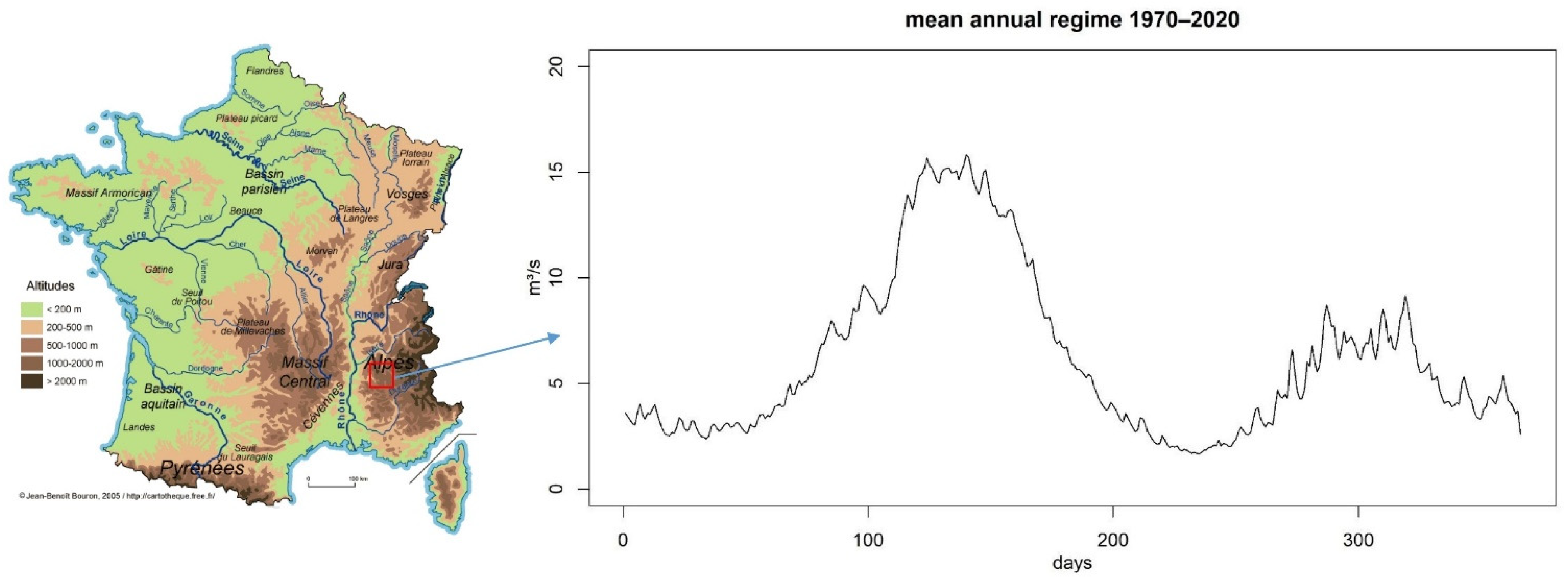
2.1. Description of the Watershed

A small watershed in the French Alps, the river Souloise at Infernet, is used here as an example for the test of the proposed methodology. Figure 1 illustrates the location of the watershed together with its mean annual regime. The basin has a drainage area of 214 km2. The Souloise is an alpine river, with a nival regime as illustrated in Figure 1. Additional descriptive information of the watershed is reported in Table 1. At the location of the watershed, temperature, precipitation and flow observations were easily available for the period 1970–2013 when the experience was first conducted. This is why all of the computations are made on the 1970–2013 period even if the data could be extended to a more recent period. Over this period, the lowest observed flow is 0.56 m3/s on the 4 November 1985 and the highest is 98 m3/s on the 30 September 1991. This watershed has been chosen for this methodological experiment for various reasons. Firstly, the fact that snow plays an important role in the generation of flows (cf. Table 1) was challenging for the bivariate temperature and rainfall generator, the good reproduction of flow seasonality via the hydrological model depending directly on the ability of the weather generator to produce realistic bivariate snowy events. Secondly, being a small mountainous watershed, this basin has still been preserved, to our knowledge, from any human activity which could strongly influence low water levels (for example, there is no upstream reservoir, the Souloise being in fact a tributary of the Sautet reservoir located downstream). Finally, the discharge series is considered to be of good quality, especially at low flow, due to the regular periodic visit and gauging of the field hydrologists (approximately four gaugings per year) and to a favorable location: upstream of a rocky canyon with a stable bed. These result in a reliable rating curve.

2.2. The Non-Homogenous Hidden Markov Model

A Hidden Markov Model (HMM) with state space X and observation space Y is a stochastic process indexed on time t such that:
(Xt)t≥1 is a Markov chain with state space X.
For all t ≥ 1, the distribution of Yt given (Xt)t≥1 only depends on t and Xt, and conditionally on (Xt)t≥1, the Yt’s are independent.
From a statistical point of view, however, the state sequence (Xt)t≥1 is not observed, only the Yt’s are, which is why the sequence Xt is called hidden states. The law of the Markov chain (Xt)t≥1 is determined by its initial distribution π such that, πk = P(X1 = k), where k designs state k, and its transition matrices (Q(t))t≥1.
The conditional distributions of Yt given Xt are called the emission distributions.
The model is used here to consistently simulate two variables: temperature and precipitation. Therefore, the observation space is Yt = R+ × R and Y t = Y t 1 , Y t 2 . The superscript (1) refers to precipitation and (2) refers to temperature. The transition matrix at time t in the model is given by:
Q t i j = exp P i j t 1 + l = 1 K 1 exp P i l t ,   1 j K 1 ,   1 i K
Q t i K = 1 1 + l = 1 K 1 exp P i l t ,   1 i K ,   with   K   the   number   of   states  
where Pij(t) is the probability for shifting from state i at time t to state j at time t + 1.
This is indeed a stochastic matrix, as for all 1 ≤ iK, j = 1 K Q t i j = 1   and Q(t)ij > 0. For 1 ≤ iK and 1 ≤ jK − 1, Pij is a trigonometric polynomial with known degree d and period T:
P i j t = β i j 0 + l = 1 d β i j , 2 l 1 cos 2 π T l t + β i j , 2 l sin 2 π T l t
Hence, the transition probabilities of the hidden Markov chain are a periodic function of time, which makes the Hidden Markov Model non-homogenous. This allows the model to reproduce some of the seasonal behaviours of climate variables.
Then, in order to allow for flexibility, mixtures are chosen as emission distributions. More precisely, the conditional distribution of Yt given Xt = k is
ν k t = p k m ν k , m 1 t ν k , m 2
The pkm are the weights of the mixture, satisfying pkm 0 and m = 1 M p k m = 1 . The emission distributions are defined as:
ν k m , t 1 = δ 0                                                                           1 m M 1 ε λ k m 1 + σ k t                                                 M 1 + 1 m M                                    
Thus, the marginal distribution of precipitation in state k at time t is a mixture of a Dirac mass with weight m = 1 M 1 p k m   and exponential distributions with parameters λ k m 1 + σ k t   and weights pkm, M1 + 1 ≤ mM. On the temperature side,
ν k m , t 2 = N T k t + S k t + μ k m , σ k m
so that the marginal distribution of temperature in state k at time t is a mixture of gaussian distributions, with variances σ k m 2 . The parameter μkm is a mean parameter that depends on both the state k and the component m, Tk(t) is a function corresponding to the temperature trend, modeled by a continuous, piecewise linear function and Sk(t) is a trigonometric polynomial with degree d corresponding to the seasonal cycle of temperature. Therefore, the temperature is generated through a mixture of gaussian distributions with a variance depending on the state k and on the component m of the mixture and a seasonal mean with a trend component. Both the trend and the seasonality of temperature are allowed to depend on the hidden state, hence the subscript k. Equation (4) shows that, in each state and each component of the mixture, precipitation and temperature are independent, but of course they are not globally independent.
The inference of the model parameters is based on maximum likelihood by use of the EM algorithm [24]. The model necessitates the specification of so-called hyper-parameters: the number of hidden states K, the degree d of the trigonometric polynomials, which sets the complexity of the seasonality, and the numbers M and M1 of distributions in the mixtures for the emission distributions. They must be chosen according to the parsimony principle in order to ensure a balance between the complexity of the model, conditioning its ability to capture the statistical properties of the data and the necessity of avoiding overfitting and maintaining the interpretability of the hidden states. The selection of the number of states, which is by far the most important hyper-parameter because the number of parameters of the model is quadratic in K, is made according to a BIC criterion [25]. To do so, models with four to seven states are calibrated against the observations, and the BIC criterium estimated. The model with seven states is the one which minimises the criterium. For the other hyper-parameters, d = 2, M = 4 and M1 = 2 are used based on previous experience of univariate models.

2.3. The Hydrological Model MORDOR

The MORDOR (MOdèle à Réservoirs de Détermination Objective du Ruissellement) model is a lumped conceptual rainfall-runoff model. Its structure is similar to that of many conceptual type models, with different interconnected stores. It works continuously and can be used with a time step ranging from hourly to daily. Required input data are areally averaged rainfall and air temperature. The details and the equations of the model are described in [26]. We use here the semi-distributed version of the MORDOR model that includes a spatial discretization scheme based on an elevation zone approach. In the Souloise watershed application the model was discretized into eight different elevation zones ranging from 1100 to 2430 m.
The model is composed for each elevation zone of:
-
a snow accumulation function calculated from the temperature and a rain–snow transition curve;
-
a snowmelt function based on an improved degree-day formulation;
-
an evaporation function that determines the potential evaporation as a function of the air temperature;
-
a rainfall excess and soil moisture accounting storage that contribute to the actual evaporation and to the direct runoff;
-
an evaporating storage filled by a part of the indirect runoff component that contributes to the actual evaporation;
-
an intermediate storage that determines the partitioning between a direct runoff, an indirect runoff and the percolation to a deep storage.
The last two components considered as global and calculated on the catchment scale are:
-
a deep storage that determines a baseflow component;
-
a unit hydrograph that determines the routing of the total runoff.
An automatic calibration scheme based on a genetic algorithm has been used to optimize the free parameters (14 free parameters were used in this case). It has been calibrated at EDF (Electricité de France) for operational inflow and for the forecasting of long-term water resources. Indeed, as mentioned earlier, the Souloise river is a tributary of a dam operated by EDF and located downstream. The multi-criterion composite objective function used during the calibration process [26] is designed to make a triple focus on time series, seasonal streamflow and flow duration curve. This objective function has been successfully used to optimize the parameters of numerous models, allowing a good trade-off between the day-to-day performance of the model and a good representation of the highest observed discharges. In this case, no specific criterion is designed to help the model fit the low flows properties, and this is the main reason why the model exhibits an important bias on the very low flows (see Section 3 below). The model could be recalibrated with a criterion allowing a better fit for low flows. The choice of such a criterion is not an easy task and this will be undoubtedly an issue if it comes someday to move on to real impact studies.
For the moment, the model will be used to produce river flow time series corresponding to the temperature and rainfall time series simulated by the bivariate generator previously described. In a way, we test the realism of the climate generator via the filter of the hydrological model. For this same reason, no calibration versus validation protocol has been designed for the hydrological model, and the MORDOR model has been used as calibrated by EDF for its operational needs.

2.4. Simulation Strategy and Return Level Estimation

As previously mentioned, the aim of the study is to simulate a large number of river flow time series in order to estimate rare low flow events. To do so, the stochastic model is first calibrated with the temperature and precipitation time series and used to simulate 1000 new temperature and precipitation time series. Then, these simulated time series are provided as inputs to the hydrologic MORDOR model in order to produce 1000 river flow time series. Depending on the total number N of years in the time series used for the model calibration, this strategy allows the generation of N × 1000 years of river flow.
From this large sample, the desired return level is estimated empirically. Coming back to the definition of a A-year return level, which is a value exceeded on average once in A years, the 100-year return level, for example, corresponds to the quantile 1 − 1/(nby × 100) of the distribution, nby being the number of events per year. Here, the desired extreme value is a minimum, which means that the A-year return level corresponds to a value non exceeded on average once in A years, and the 100-year return level corresponds to the 1/(nby × 100) quantile of the distribution. Such quantiles are so high or low that they are generally estimated by the observed maximum or minimum, which is why the statistical extreme value theory is used for return level estimations. But here, because the sample is very large, this empirical estimation is achievable. Then, the confidence interval is obtained by a non-parametric bootstrap: 1000 samples of the total number of simulated low flows are drawn with replacement from the original sample, and the quantile corresponding to the 100-year return level is estimated for each sample. Having done that, one attains a distribution of 1000 possible 100-year return values. From this distribution, different methods are proposed in the literature to estimate a confidence interval [27]. The simplest one is to estimate the confidence bounds as the corresponding quantiles of the bootstrap distribution (quantiles α/2 and 1 − α/2 for a 100(1 − α)% confidence interval). The normal approximation consists of considering the distribution obtained by the bootstrap as normal, and the confidence interval bounds are estimated as θ ^ + θ ^ θ ¯ b ±   z α 2 s d θ ^ b , where θ ^ is the value obtained from the original sample, θ ¯ b is the mean of the values given by the bootstrap samples, s d θ ^ b is their standard deviation and zα/2 is the α/2 quantile of the normal distribution, 100(1 − α)% being the confidence level. Another approach called “basic bootstrap” consists in using the bootstrap estimates to compute the distribution of the differences between each estimate and the value obtained from the original sample. Then, this distribution is considered as an estimation of the distribution of the differences between the “real” return level value and its estimation. The confidence intervals are then built following this consideration.
Then, depending on the period for which the return level estimation is made, the stochastic model is calibrated either with the observed time series, if the estimation is for the current climate, or with the time series taken from the climate projections and bias-adjusted, if the estimation is for a future period.

3. Results

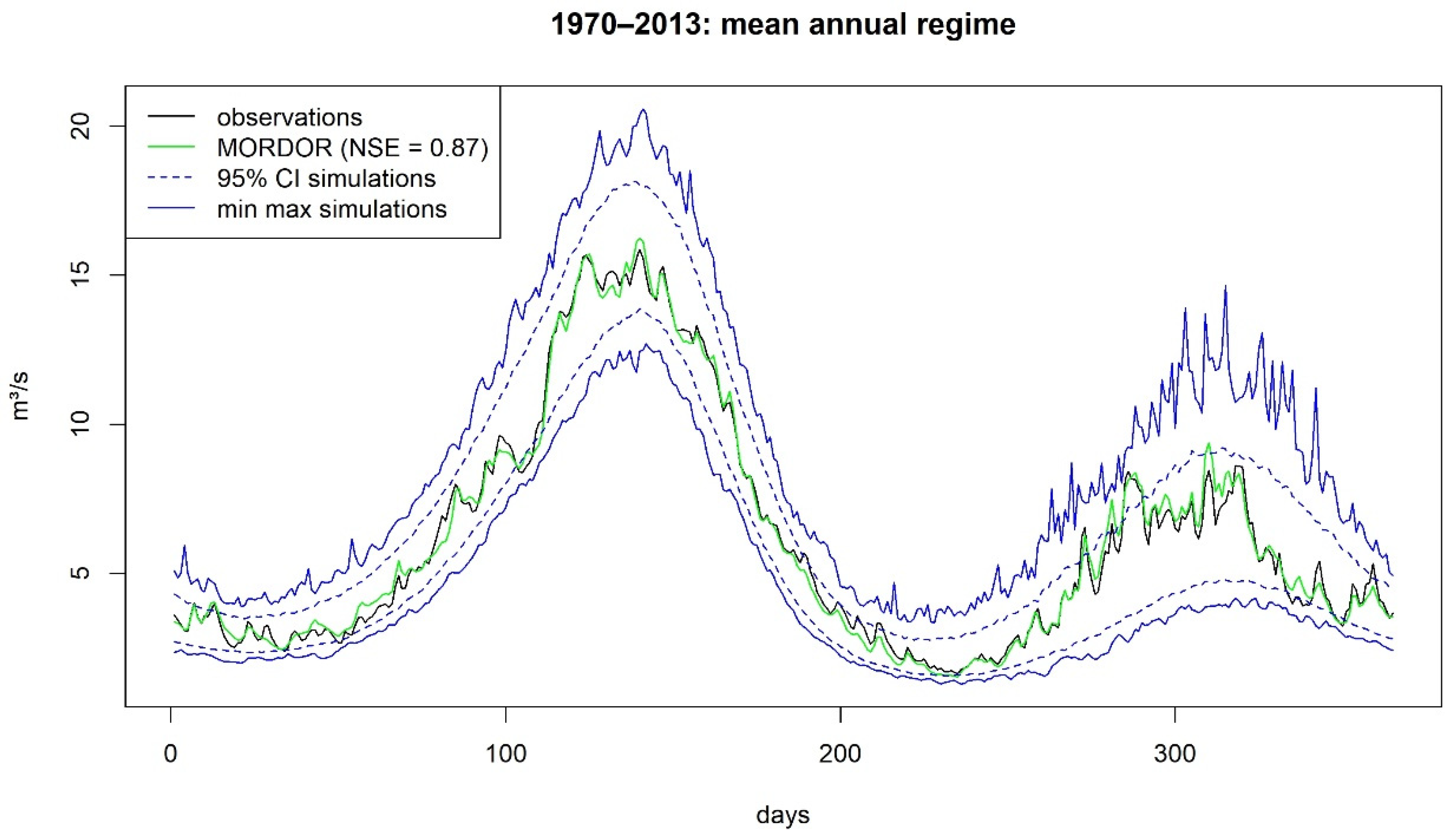
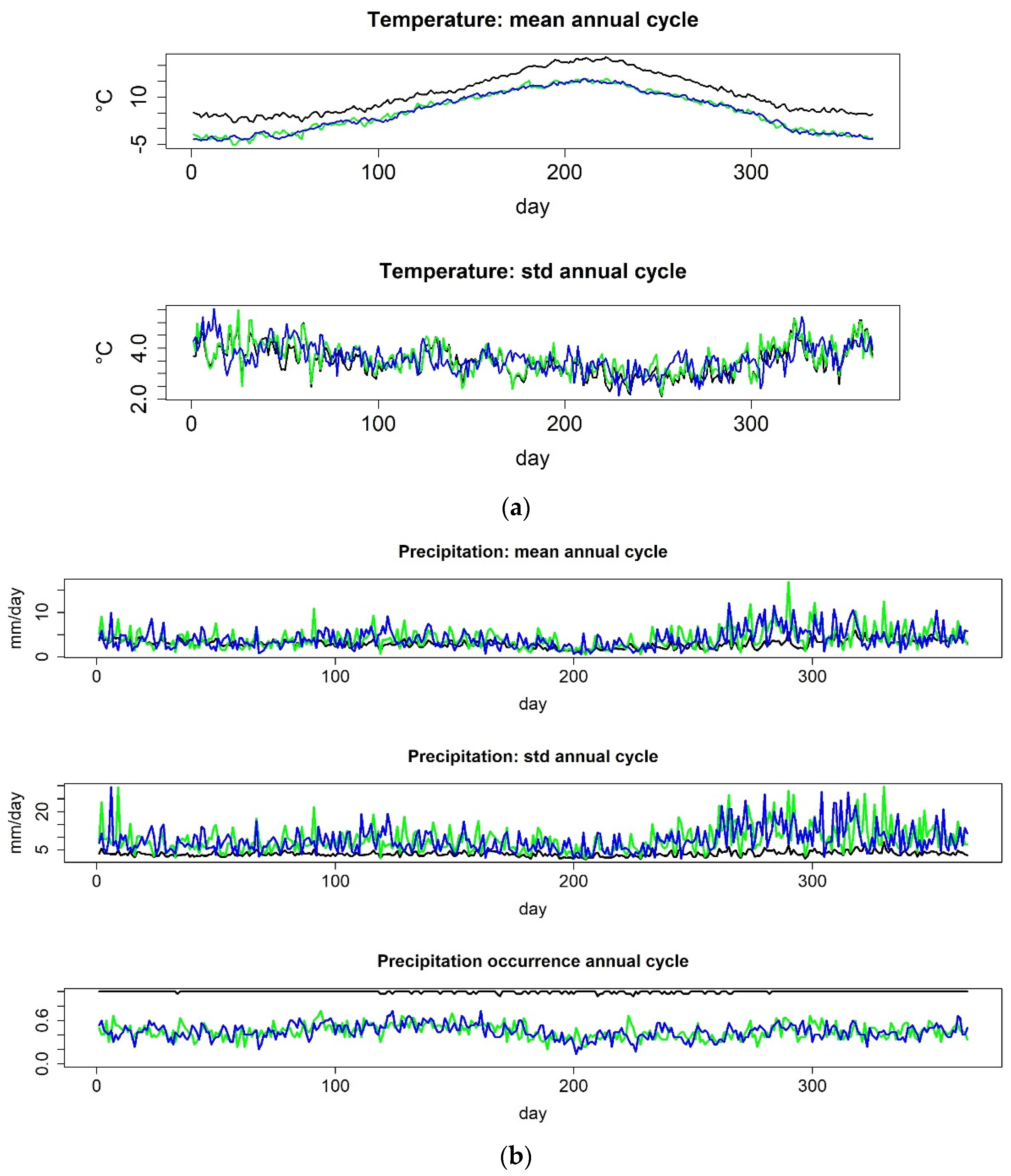
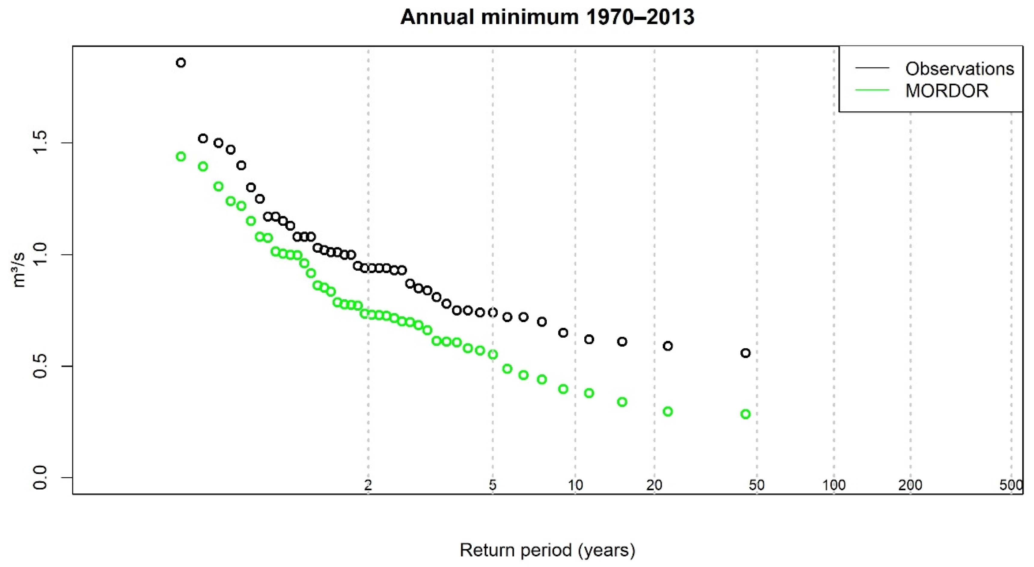
3.1. Validation over the Historical Period

The first step has thus been devoted to the validation of the simulations. Starting from the observed precipitation and temperature time series for the Souloise at Infernet watershed covering the period 1970–2013, the bivariate stochastic model has been calibrated and used to simulate 1000 equivalent 44-year time series of joint precipitation and temperature evolutions.
These time series have then been used as inputs for the hydrological MORDOR model to produce 1000 44-year river flow time series. This set of simulations has been compared to the observations over the period 1970–2013 in order to check that they correctly reproduce the observed features while giving potentially higher and lower values than observed. The 95% confidence interval is considered here together with the absolute minimum and maximum because the aim is to analyze the model behavior through the largest possible range of simulations. Figure 2 shows the comparison of the mean annual regime as obtained from the observations with the range of mean annual regimes given by the simulations. The first validation concerns the MORDOR model, through the comparison of the observed annual mean regime to that obtained with MORDOR while forced with the observed temperature and precipitation evolutions over the observation period. It can be seen in Figure 2 that, firstly, MORDOR faithfully reproduces the mean annual regime (comparison of the black and green curves: the Nash-Sutcliffe coefficient of Efficiency—NSE—is also reported in the caption) and, secondly, the 1000 simulations encompass the observations, with a realistic behavior and an expected capacity of simulating higher and lower flows than observed. The dotted lines represent the 95% confidence interval obtained from the simulations. The observation-driven MORDOR regime is outside of the 95% interval approximately 8% of the time, which, considering the temporal dependence, is quite correct.
If we now focus on the lowest flows, Figure 3 shows that MORDOR tends to underestimate the lowest values.
Therefore, from now on, the flow time series obtained with MORDOR forced with the observed temperature and precipitation will be considered as the observations, so that the comparison with the stochastically generated sample can be fair. In this time series, the observed minimum is 0.29 m3/s and the observed maximum 106.7 m3/s.
Then, the distributions of low flow durations for different thresholds used to define low flows (9th, 7th, 5th and 3rd percentiles of observation-based flows estimated by MORDOR) are compared between observations and stochastic simulations (Figure 4). The observed sequences’ proportions lie inside the 95% confidence interval of that given by the simulations, whatever the duration, which means that the generation is able to correctly reproduce the observed proportions of sequences of different durations, even the longest ones, and can even simulate longer low flow periods, at least until a duration of 60 days.

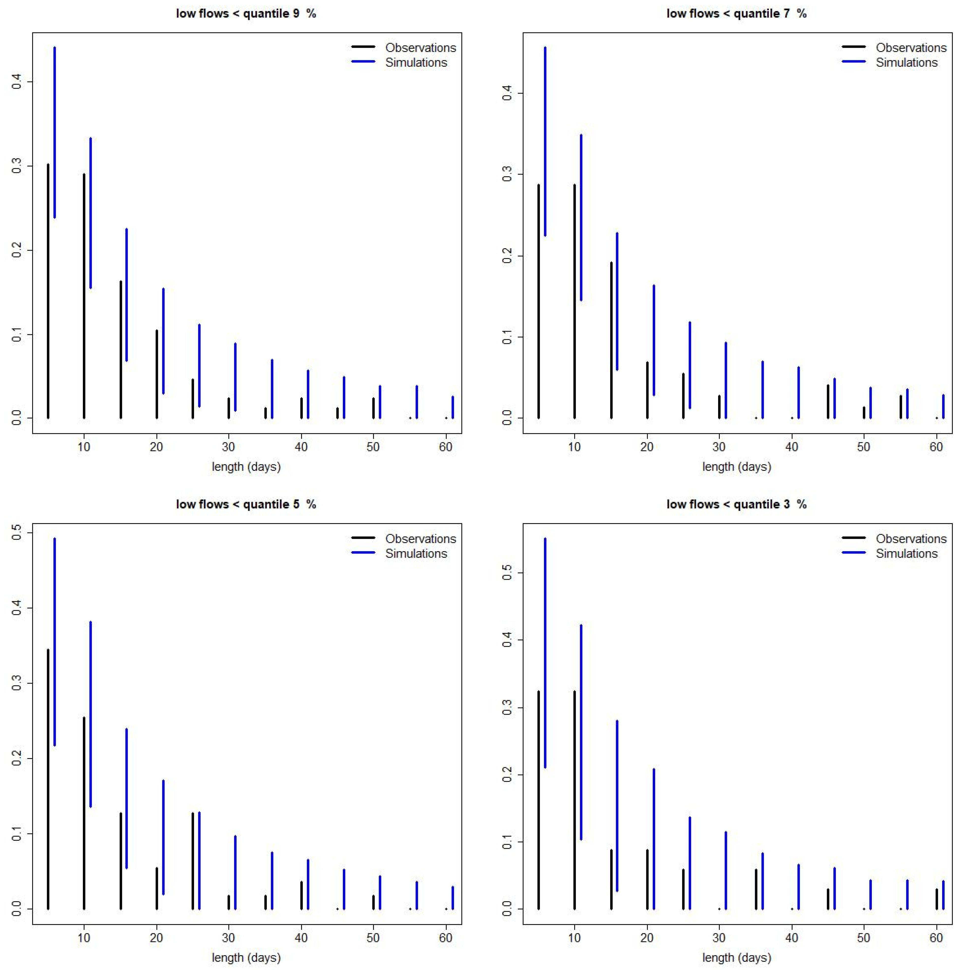
3.2. Extreme Low Flow Estimation

Once the capacity of the simulations to reproduce low flows has been checked, it seems reasonable to use the large sample produced, which now consists of 44,000 years, in order to estimate rare events. If the 5th percentile of the MORDOR-based observed distribution is used to select low flow sequences (which corresponds to 0.85 m3/s), 57 low flow events are identified from these observations, which means around 1.29 event per year on average, with minimum flow over the events ranging from 0.29 m3/s to 0.84 m3/s. In the stochastically simulated large sample, the same threshold yields to the selection of 45598 low flow events, which equates to approximately 1.04 events per year, with minimum flow over the events ranging from 0.21 m3/s to 0.85 m3/s. The estimation of an extreme low flow is based on the distribution of the minimum flows of each event. As far as very low flows are concerned, the data driven MORDOR simulation gives one occurrence of a flow lower than 0.3 m3/s over 44 years (around 2.3%) while the stochastically simulated sample presents 126 such occurrences in the 44,000 simulated years (around 0.3%). It is difficult at this point to decide if the stochastic model tends to underestimate the proportion of very low flows or if the observed one is exceptional and would have been unique even in a longer observation period; it is probably both.
If the 100-year return level is now estimated as the 1/(nby × 100) percentile of the low flow distribution as described in the previous section, then, as in the simulated sample, there are 45,598 values with 1.04 events per year on average, the 1/(1.04 × 100) = 0.96% quantile has to be estimated. This value is 0.34 m3/s.
The estimation of a confidence interval around the value is here based on the bootstrap described in the previous section. All of the three approaches considered to derive the lower and upper bounds give similar results, and the 100-year extreme low flow is then 0.342 m3/s within the 70% confidence interval [0.340; 0.344]. The 70% confidence interval is conventionally considered here, in line with the requirements of the regulation.
This estimation is not sensitive to the threshold chosen for the identification of the low flow sequences. If the 10th percentile is chosen instead of the 5th, 99 sequences are identified in the observation-driven MORDOR time series (that is 2.25 per year on average) and 88,633 (that is 2.01 per year on average) in the stochastically simulated sample. The percentile corresponding to the 100-year return level is again 0.342 m3/s with the same 70% confidence interval.
Because MORDOR tends to underestimate the lowest flows, one way of retrieving a value compatible with the observations could be to add to this value the difference between the observed lowest flow and the MORDOR-simulated one (0.56 − 0.29 = 0.27). Then, the 100-year return level can be estimated as 0.612 m3/s [0.610; 0.614].

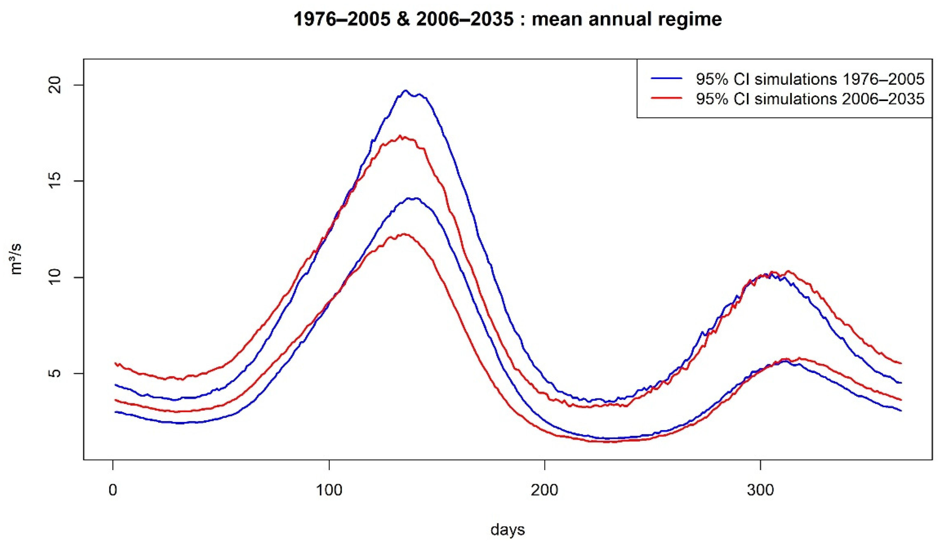
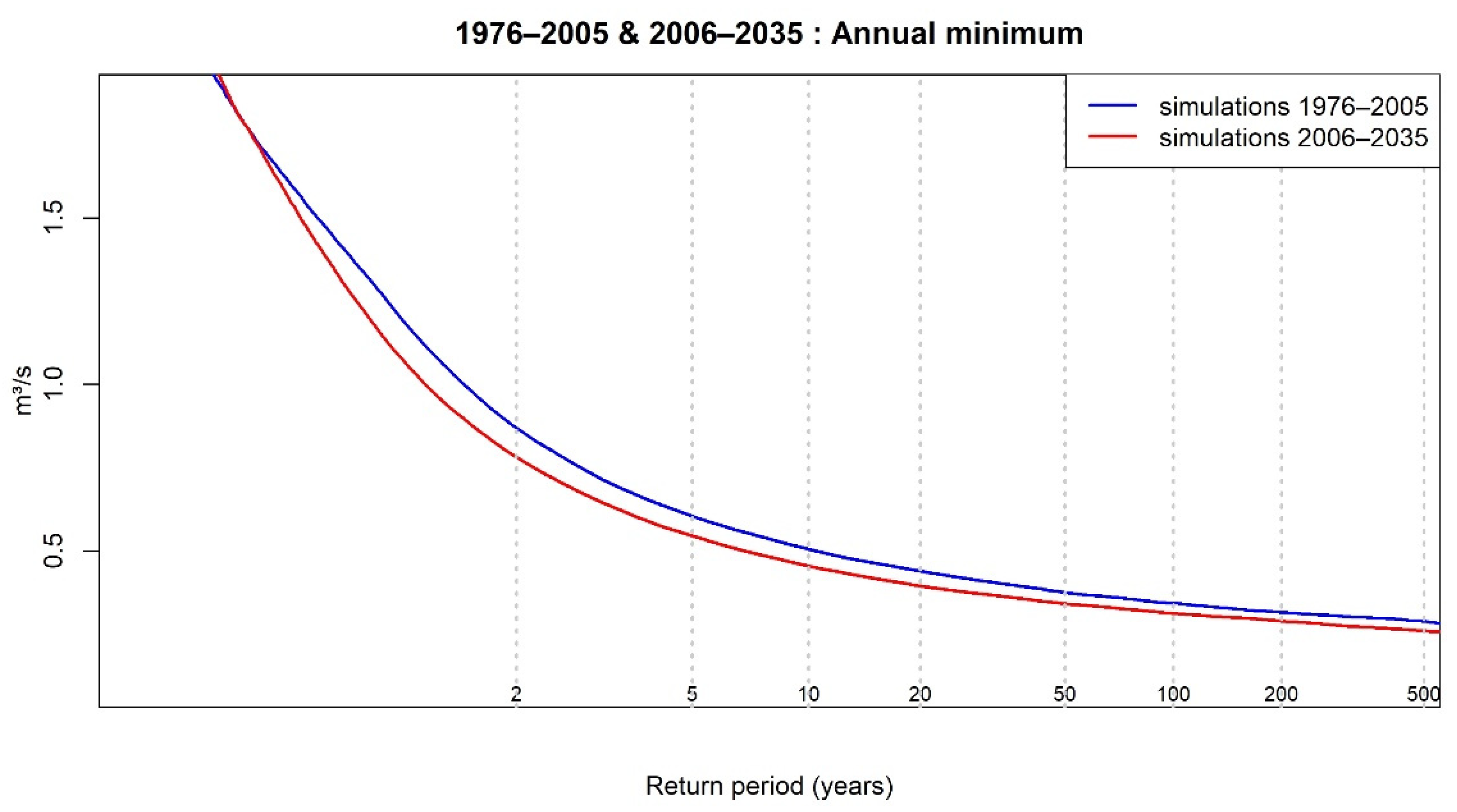
3.3. Future Extreme Low Flow

The framework previously developed and tested to estimate extreme low flow values can be used to study the impact of climate change on this type of extreme. To do so, the stochastic model is calibrated to reproduce a large sample of temperature and precipitation time series given by climate projections downscaled at the watershed level. This is illustrated in the following by the use of the projection under scenario RCP8.5 made by model BNU-ESM in the framework of the project CMIP5 (5th Coupled Model Intercomparison Project) in support of the 5th IPCC (Intergovernmental Panel on Climate Change) assessment report. This model has been chosen because it projects a warming in summer over France which is around the median of the projections of the CMIP5 ensemble. Only one projection is used here because the aim is to illustrate the application of the proposed approach in the climate change context, not to study the impact of climate change on extreme low flow for this basin. In the latter case, it would have been necessary to use an ensemble of projections and not only one. This will be studied in future work, once the methodology is in place.
The first task has then been to extract the climate model projection data for the grid point nearest to the location of the watershed. This has been made for the period 1976–2035. The time series of precipitation and temperature have first been bias-adjusted against the observations with the commonly used CDFt method [28]. This method aims at adjusting the distribution of the variable given by the climate projection so that it matches the observed distribution. The adjustment is made independently for temperature and precipitation, and month by month in order to deal with the seasonality of the distributions. Figure 5 compares the annual cycles before and after adjustment, compared to the observations over the period 1976–2005, for temperature mean and standard deviation and for precipitation mean, standard deviation and proportion of rainy days, and shows that the bias adjustment is efficient.
Then, the bivariate stochastic model is fitted to the bias-adjusted temperature and precipitation time series over the whole 1976–2035 period in order to simulate 1000 replicates of these 60-year time series, then used as input for the MORDOR model. The (GCM+CDFt+HMM+MORDOR) whole framework produces 1000 streamflow series over the period 1976–2035 that can be split in two sub-periods: the historical period 1976–2005 and the future period 2006–2035.
Figure 6 shows the evolution of the average annual regime between the period 1976–2005 and the period 2006–2035: flows tend to increase in winter due to the rise in temperature (less snowfall). For the same reasons (decrease in the snowpack), snowmelt is less important in the spring while occurring earlier, once again due to the rise in temperature. In summer, the low flows tend to decrease because of the earlier snowmelt and the rise of the evapotranspiration.
Figure 7 makes a special focus on annual minimum, showing the decrease in the extreme low flows.
In order to further quantify the observed decrease in the lowest flows, different low flow return levels are successively estimated as the 1/(nby × N) quantile of the distribution of low flows over each period, the historical period 1976–2005 and the future period 2006–2035, N being the return period. Table 2 summarizes the results. It shows both an increase in the mean number of events per year and a significant decrease in the extreme low flows. For instance, the 100-year return level for the historical period becomes a 50-year return level in the future period, and the 200-year return level is close to the 100-year return level in the future.

4. Discussion

In this paper, a methodology designed to estimate extreme low flows has been proposed and tested. Since for these events, the application of the extreme value theory is not theoretically justified, the proposed approach consists in creating a very large sample of flow time series equivalent to the observed one in order to be able to do more robust empirical statistics. A bivariate stochastic model based on a non-homogenous hidden Markov model is used to produce a very large sample of temperature and precipitation time series, which are in turn transformed into river flow thanks to a rainfall runoff model.
The approach has first been validated and proven to be useful both to estimate historical extreme low flows and to study the impact of climate change on these extremes. However, different weaknesses have been identified. First, the rainfall-runoff model tends to underestimate the low flows. Secondly, the lowest flows produced with precipitation and temperature given by the stochastic generator seem to be less frequent than observed. Further investigations proved that the duration of the longest sequences seem to be underestimated, too. With these biases in mind, the potential of the proposed framework to estimate extreme low flows and their changes in the climate change context has nevertheless been demonstrated. This study is not devoted to the understanding of the impact of climate change on extreme low flows. Such a study would necessitate the use of an ensemble of climate models, not just the one considered here. However, the merit of the proposed framework is to present another methodology to estimate the climate change impact on extreme low flow values. This methodology can represent an alternative to [6] which relies on a large ensemble of climate change factors applied to the meteorological variables used as input to runoff models. The use of climate change factors does not allow taking possible changes in variability into account, whereas the approach proposed here does. Besides, the changes in [6] are studied for the 5th and 95th percentiles of the flow distribution, again not for the rarer extremes focused on here with the proposed methodology. It also represents an extension of [7] with the use of another type of stochastic generator and another way of estimating return values.
As previously stated, the work here must be considered as a first proof of concept, and deserves further investigations. It has been shown that the choice of the threshold used to identify the low flow sequences does not impact the results. Other sensitivity experiments will be made to test the robustness of the approach. For example, the number of stochastic simulations could be questioned: how sensitive are the results to this number? Is the number of very low flows steadily increasing with the number of simulations or is there some sort of asymptotic behavior? This question had been considered in [29] in the context of different autoregressive weather generators, and the conclusion was that the essential statistics were well reproduced with only 25 simulations. However, they did not look at the extremes, as is the case here. Besides, one needs to check if this holds for a non-homogenous HMM. The stochastic model’s ability to represent very long duration sequences will also be further analyzed, and ways to improve it will be designed and tested. Then, for use in the climate change context, a real impact study would necessitate the consideration of an ensemble of projections. But, here again, possible improvements could be tested, such as the potential benefit brought if the two variables, precipitation and temperature, were jointly bias-adjusted instead of separately. Finer resolution regional climate projections could also be better adapted, due to their more realistic representation of the local climate. Finally, the setting will be applied to a larger set of watersheds with different hydrological behaviors in order to assess its ability in different contexts.

5. Conclusions

In this paper, a methodology involving stochastic generation of precipitation and temperature time series and a hydrological model has been proposed to estimate low flow return values. The very large sample of river flow obtained in this way enables the empirical estimation of return values. This approach can be applied both to observation time series, in order to estimate current climate return levels, and to downscaled climate projection outputs, in order to evaluate the impact of climate change on those rare values. The framework has been applied here to a small watershed without any large human influence. This is obviously not the common case, and climate change is far from being the only driver of river flow changes. Human influence complicates the return value estimation as well. Therefore, for future work devoted to the application of the approach in a larger hydrological context with an ensemble of climate projections, human influence on the flow management will have to be taken into account. Flow management can first be removed in order to get the most natural flow possible, but then scenarios will have to be imagined for the estimated flows to be as close to the real situation as possible.

Author Contributions

Conceptualization, S.P. and J.G.; methodology, S.P.; software, J.G. and S.P.; validation, S.P. and J.G.; investigation, S.P. and J.G.; writing—original draft preparation, S.P.; writing—review and editing, S.P. and J.G.; visualization, S.P. and J.G. All authors have read and agreed to the published version of the manuscript.

Funding

This research received no external funding.

Institutional Review Board Statement

Not applicable.

Informed Consent Statement

Not applicable.

Data Availability Statement

The data presented in this study are available within the manuscript.

Acknowledgments

We acknowledge the World Climate Research Programme’s Working Group on Coupled Modelling, which is responsible for CMIP, and we thank the climate modeling group (College of Global Change and Earth System Science, Beijing Normal University) for producing and making available their model output. For CMIP, the U.S. Department of Energy’s Program for Climate Model Diagnosis and Intercomparison provides coordinating support and leads development of software infrastructure in partnership with the Global Organization for Earth System Science Portals.

Conflicts of Interest

The authors declare no conflict of interest.

References

  1. Krysanova, V.; Vetter, T.; Eisner, S.; Huang, S.; Pechlivanidis, I.; Strauch, M.; Gelfan, A.; Kumar, R.; Aich, V.; Arheimer, B.; et al. Intercomparison of regional-scale hydrological models and climate change impacts projected for 12 large river basins worldwide—A synthesis. Environ. Res. Lett. 2017, 12, 105002. [Google Scholar] [CrossRef]
  2. Marx, A.; Kumar, R.; Thober, S.; Rakovec, O.; Wanders, N.; Zink, M.; Wood, E.F.; Pan, M.; Sheffield, J.; Samaniego, L. Climate change alters low flows in Europe under global warming of 1.5, 2, and 3 °C, Hydrol. Earth Syst. Sci. 2018, 22, 1017–1032. [Google Scholar] [CrossRef] [Green Version]
  3. Donnelly, C.; Greuell, W.; Andersson, J.; Gerten, D.; Pisacane, G.; Roudier, P.; Ludwig, F. Impacts of climate change on European hydrology at 1.5, 2 and 3 degrees mean global warming above preindustrial level. Clim. Change 2017, 143, 13–26. [Google Scholar] [CrossRef] [Green Version]
  4. Oo, H.T.; Zin, W.W.; Kyi, C.T. Analysis of Streamflow Response to Changing Climate Conditions Using SWAT Model. Civ. Eng. J. 2020, 6, 194–209. [Google Scholar] [CrossRef]
  5. AlSafi, H.I.J.; Sarukkalige, P.R. The application of conceptual modelling to assess the impacts of future climate change on the hydrological response of the Harvey River catchment. J. Hydro-Environ. Res. 2020, 28, 22–33, ISSN 1570-6443. [Google Scholar] [CrossRef]
  6. Kay, A.L.; Watts, G.; Wells, S.C.; Allen, S. The impact of climate change on U.K. river flows: A preliminary comparison of two generations of probabilistic climate projections. Hydrol. Process. 2020, 34, 1081–1088. [Google Scholar] [CrossRef]
  7. Alodah, A.; Seidou, O. Assessment of Climate Change Impacts on Extreme High and Low Flows: An Improved Bottom-Up Approach. Water 2019, 11, 1236. [Google Scholar] [CrossRef] [Green Version]
  8. Coles, S.; Bawa, J.; Trenner, L.; Dorazio, P. An Introduction to Statistical Modeling of Extreme Values; Springer Series in Statistics; Springer: Berlin/Heidelberg, Germany, 2001. [Google Scholar]
  9. Leadbetter, M.R. Extremes and local dependence in stationary sequences. Z. Wahrscheinlichkeitstheorie Verw. Gebiete 1983, 65, 291–306. [Google Scholar] [CrossRef]
  10. Richardson, C.W. Stochastic simulation of daily precipitation, temperature, and solar radiation. Water Resour. Res. 1981, 17, 182–190. [Google Scholar] [CrossRef]
  11. Wilks, D.S.; Wilby, R.L. The weather generation game: A review of stochastic weather models. Prog. Phys. Geogr. 1999, 23, 329–357. [Google Scholar] [CrossRef]
  12. Fletcher, C.; Naveau, P.; Allard, D.; Brisson, N. A stochastic daily weather generator for skewed data. Water Resour. Res. 2010, 46, W07519. [Google Scholar] [CrossRef]
  13. Vrac, M.; Stein, M.; Hayhoe, K. Statistical downscaling of precipitation through nonhomogeneous stochastic weather typing. Clim. Res. 2007, 34, 169–184. [Google Scholar] [CrossRef]
  14. Zucchini, W.; Guttorp, P. A hidden Markov model for space-time precipitation. Water Resour. Res. 1991, 27, 1917–1923. [Google Scholar] [CrossRef]
  15. Kirshner, S. Modeling of Multivariate Time Series Using Hidden Markov Models. Ph.D. Thesis, University of California, Irvine, CA, USA, 2005. [Google Scholar]
  16. Ailliot, P.; Pene, F. Consistency of the maximum likelihood estimate for non-homogeneous markov-switching models. ESAIM Probab. Stat. 2015, 19, 268–292. [Google Scholar] [CrossRef] [Green Version]
  17. Ailliot, P.; Monbet, V. Markov-switching autoregressive models for wind time series. Environ. Model. Softw. 2012, 30, 92–101. [Google Scholar] [CrossRef] [Green Version]
  18. Hugues, J.P.; Guttorp, P. A class of stochastic models for relating synoptic atmospheric patterns to regional hydrologic phenomena. Water Resour. Res. 1994, 30, 1535–1546. [Google Scholar] [CrossRef]
  19. Hugues, J.P.; Guttorp, P.; Charles, S.P. A non-homogeneous hidden Markov model for precipitation occurrence. J. R. Stat. Soc. Ser. C 1999, 48, 15–30. [Google Scholar] [CrossRef] [Green Version]
  20. Peleg, N.; Fatichi, S.; Paschalis, A.; Molnar, P.; Burlando, P. An advanced stochastic weather generator for simulating 2-d high-resolution climate variables. J. Adv. Modeling Earth Syst. 2017, 9, 1595–1627. [Google Scholar] [CrossRef]
  21. Dubrovsky, M.; Huth, R.; Dabhi, H.; Rotach, M.W. Parametric gridded weather generator for use in present and future climates: Focus on spatial temperature characteristics. Theor. Appl. Climatol. 2020, 139, 1031–1044. [Google Scholar] [CrossRef]
  22. Touron, A. Consistency of the maximum likelihood estimator in seasonal hidden markov models. Stat. Comput. 2019, 29, 1055–1075. [Google Scholar] [CrossRef] [Green Version]
  23. Alodah, A.; Seidou, O. The adequacy of stochastically generated climate time series for water resources systems risk and performance assessment. Stoch. Environ. Res. Risk Assess. 2019, 33, 253–269. [Google Scholar] [CrossRef]
  24. Dempster, A.P.; Laird, N.M.; Rubin, D.B. Maximum likelihood from incomplete data via the EM algorithm. J. R. Stat. Soc. Ser. B 1977, 39, 1–22. [Google Scholar] [CrossRef]
  25. Schwarz, G. Estimating the dimension of a model. Ann. Stat. 1978, 6, 461–464. Available online: http://www.jstor.org/stable/2958889 (accessed on 25 October 2021). [CrossRef]
  26. Garavaglia, F.; Le Lay, M.; Gottardi, F.; Garçon, R.; Gailhard, J.; Paquet, E.; Mathevet, T. Impact of model structure on flow simulation and hydrological realism: From a lumped to a semi-distributed approach. Hydrol. Earth Syst. Sci. 2017, 21, 3937–3952. [Google Scholar] [CrossRef] [Green Version]
  27. Panagoulia, D.; Economou, P.; Caroni, C. Stationary and nonstationary generalized extreme value modelling of extreme precipitation over a mountainous area under climate change. Environmetrics 2014, 25, 29–43. [Google Scholar] [CrossRef]
  28. Michelangeli, P.-A.; Vrac, M.; Loukos, H. Probabilistic downscaling approaches: Application to wind cumulative distribution functions. Geophys. Res. Lett. 2009, 36, L11708. [Google Scholar] [CrossRef]
  29. Guo, T.; Mehan, S.; Gitau, M.W.; Wang, Q.; Kuczek, T.; Flanagan, D.C. Impact of number of realizations on the suitability of simulated weather data for hydrologic and environmental applications. Stoch. Environ. Res. Risk Assess. 2017, 32, 2405–2421. [Google Scholar] [CrossRef]
Figure 1. Location of the watershed and mean annual regime over the observation period 1970–2013.
Atmosphere 13 00164 g001
Figure 2. Observed mean annual regime over period 1970–2013 (black curve) compared to the same regime as simulated by the MORDOR model using observed precipitation and temperature (green curve) and to the range of the 1000 simulations (blue curves: simulated minimum and maximum regimes, dotted 95% confidence interval obtained from the simulations).
Atmosphere 13 00164 g002
Figure 3. Comparison of the distributions of the lowest flows as observed (black dots) and simulated with MORDOR using observed temperature and precipitation (green dots) over period 1970–2013.
Atmosphere 13 00164 g003
Figure 4. Proportions of low flow sequences of different durations (durations lower than 5 days, between 5 and 10 days, …, between 55 and 60 days) in the time series computed with MORDOR using observed precipitation and temperature (black bars) and 95% interval of the same proportions given by MORDOR using the stochastic simulations of precipitation and temperature (blue segments) for different thresholds defining low flows (quantile 9, 7, 5 and 3% of the observation-based flows).
Atmosphere 13 00164 g004
Figure 5. (a) mean and standard deviation annual cycles of temperature over period 1976–2005 given by the raw climate projection (black), the observations (blue) and the bias adjusted-climate projection (green). (b) same as (a) but for precipitation, with the addition of the annual cycle of the proportion of rainy days.
Atmosphere 13 00164 g005
Figure 6. Mean annual regime: range of the 1000 simulations obtained with the whole framework (GCM+CDFt+HMM+MORDOR) (95% confidence interval): over period 1976–2005 (blue curves) and period 2006–2035 (red curves).
Atmosphere 13 00164 g006
Figure 7. Annual minimum: sorted values of the 1000 simulations obtained with the whole framework (GCM+CDFt+HMM+MORDOR): over period 1976–2005 (blue curves) and period 2006–2035 (red curves).
Atmosphere 13 00164 g007
Table 1. General descriptive information of the watershed (average values over the period 1970–2013).
Hydrological Budget (mm/Year)Descriptors
Precipitation1421Drainage Area214 km2
Rainfall911Mean Elevation1628 m
Snow 510Maximum Elevation2790 m
Actual Evapotranspiration522Minimum Elevation854 m
Runoff899
Table 2. Different return levels for low flows for each sub-period with their 70% bootstrap confidence interval in brackets.
1976–20052006–2035
Mean number of events per year0.801.02
2-year return level0.743 [0.742; 0.744]0.679 [0.678; 0.681]
10-year return level0.496 [0.495; 0.498]0.448 [0.446; 0.450]
20-year return level0.436 [0.434; 0.438]0.392 [0.390; 0.394]
50-year return level0.374 [0.371; 0.377]0.340 [0.338; 0.342]
100-year return level0.342 [0.340; 0.344]0.311 [0.309; 0.314]
200-year return level0.315 [0.312; 0.318]0.289 [0.286; 0.292]
Publisher’s Note: MDPI stays neutral with regard to jurisdictional claims in published maps and institutional affiliations.

