


Contribution of Airplane Engine Emissions on the Local Air Quality around Stuttgart Airport during and after COVID-19 Lockdown Measures


Abstract
1. Introduction
2. Methodology
2.1. Measurement Phases
2.1.1. Phase 1—No Flight Operation
2.1.2. Phase 2—Partial Flight Operation
2.1.3. Phase 3—Full Flight Operation
2.2. Flight Operation
2.3. Setup and Protocol
2.4. Measurement Devices
2.4.1. Particle Counters
2.4.2. Aethalometers
2.4.3. Gas Measurement Devices
2.4.4. Meteorological Devices
3. Results and Discussion
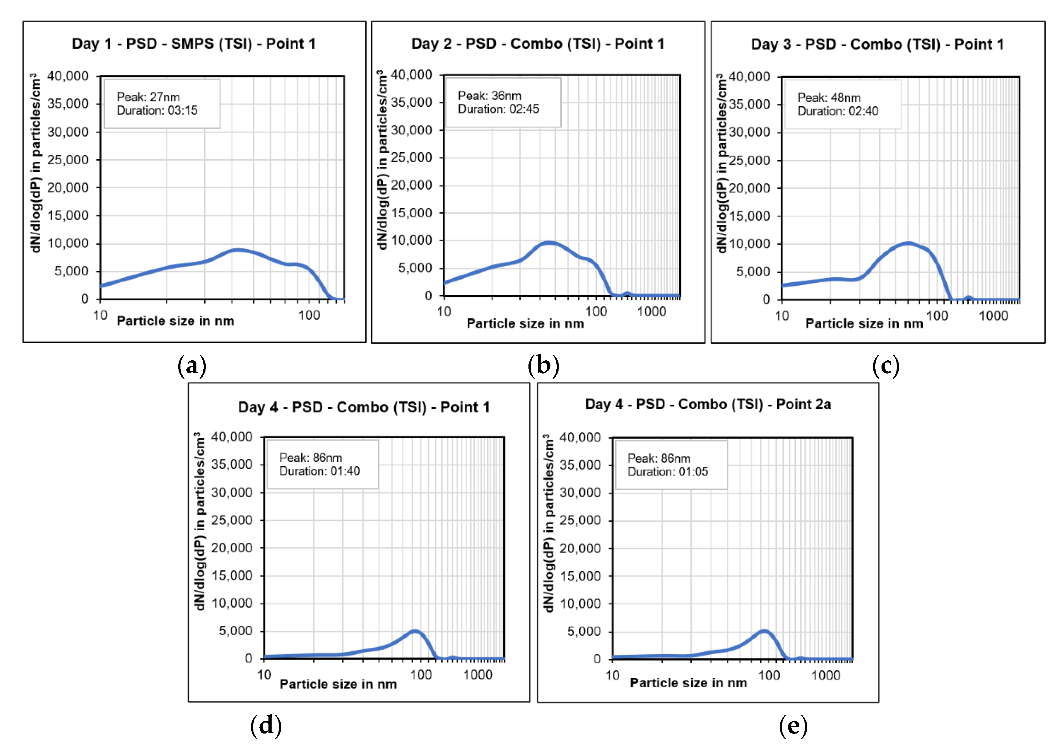
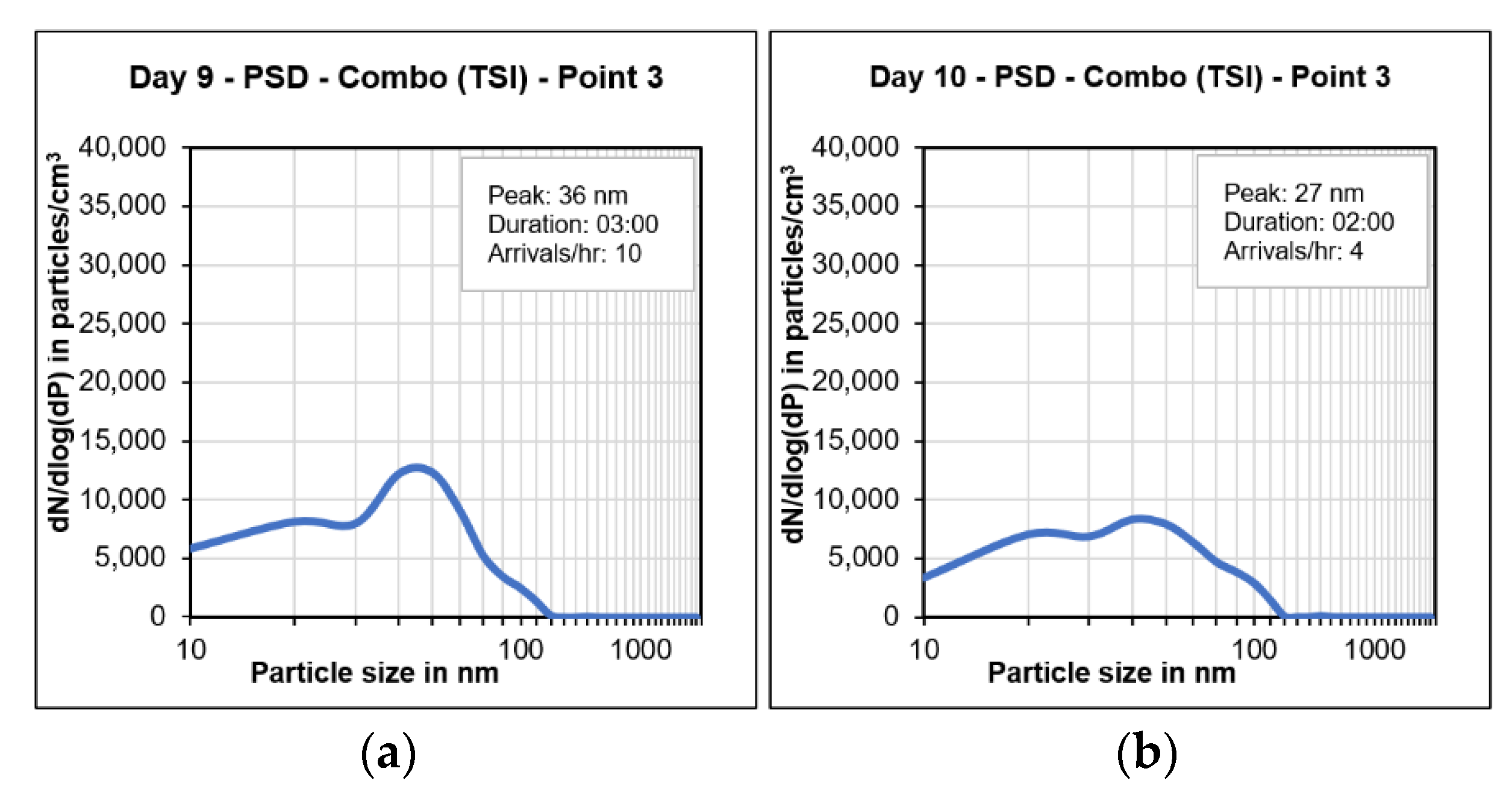
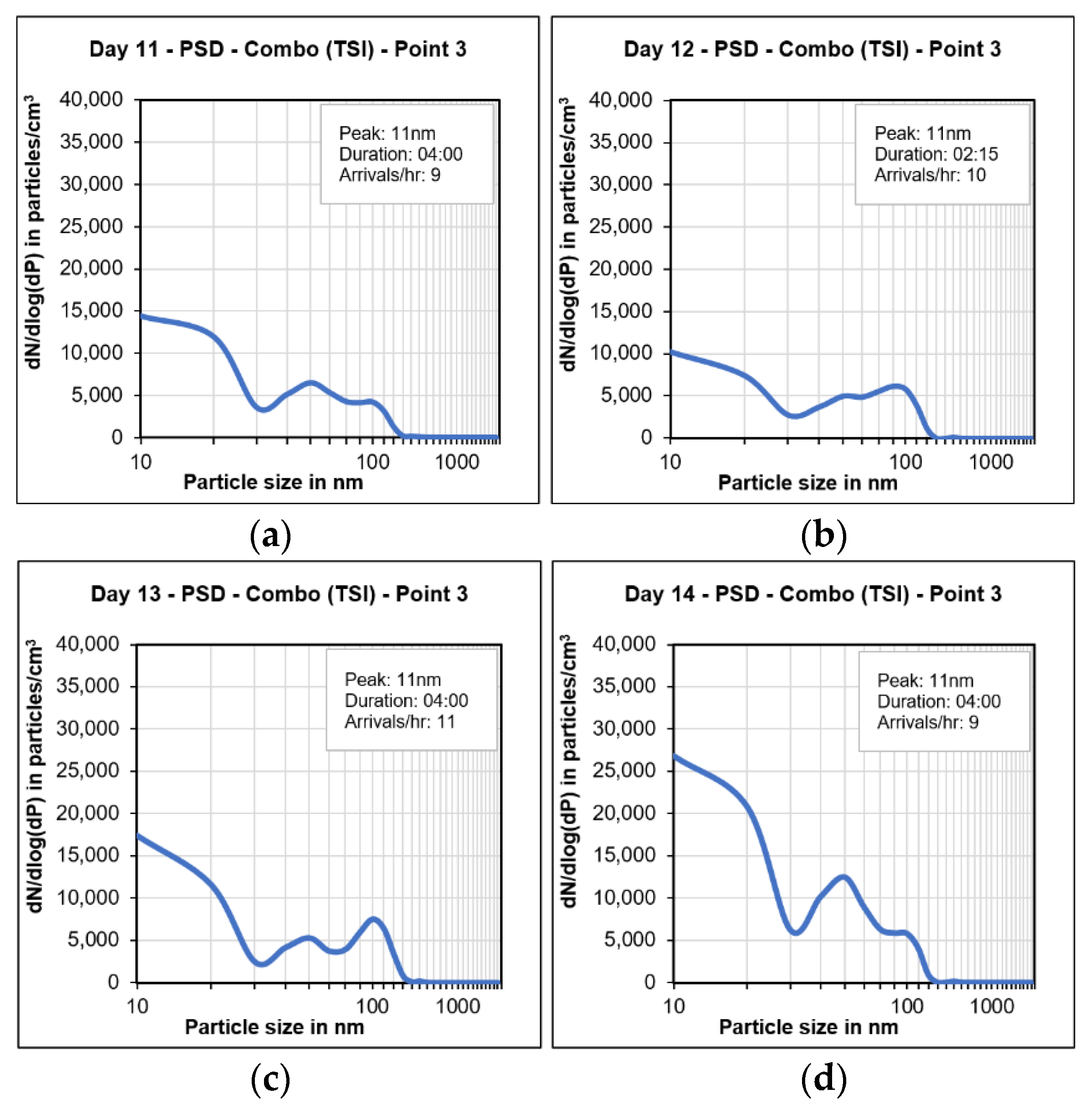
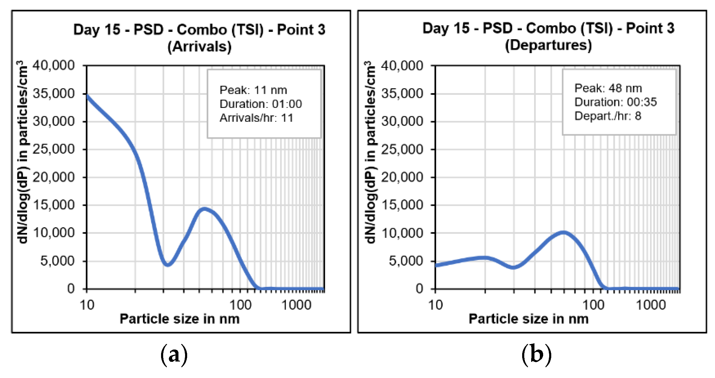
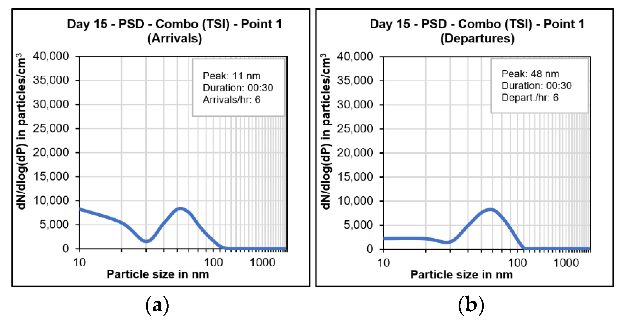
3.1. Particle Size Distribution (PSD)
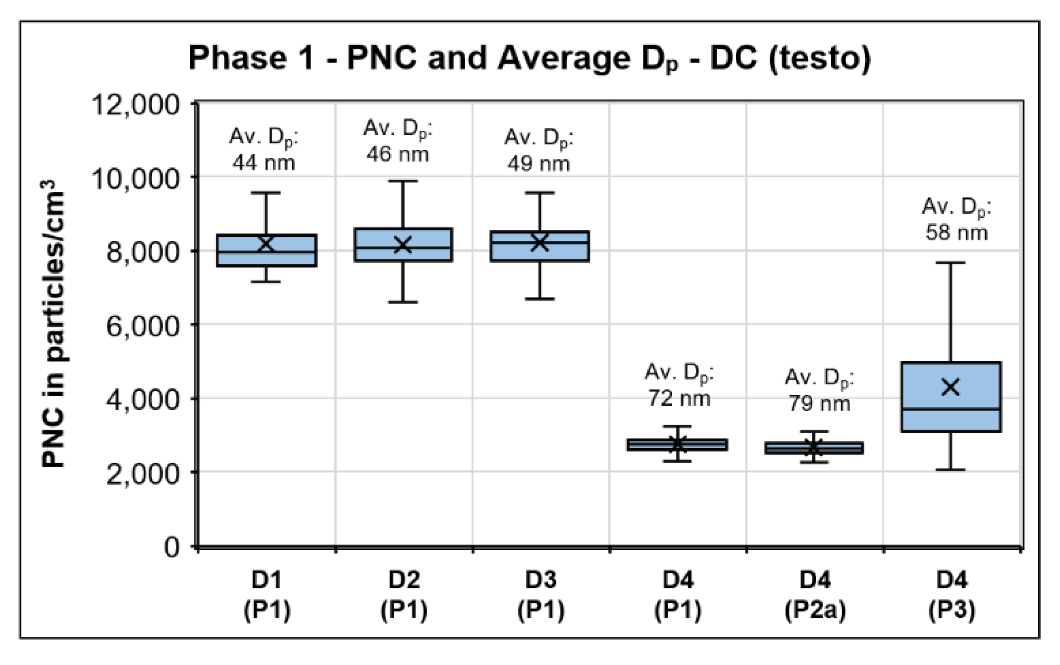
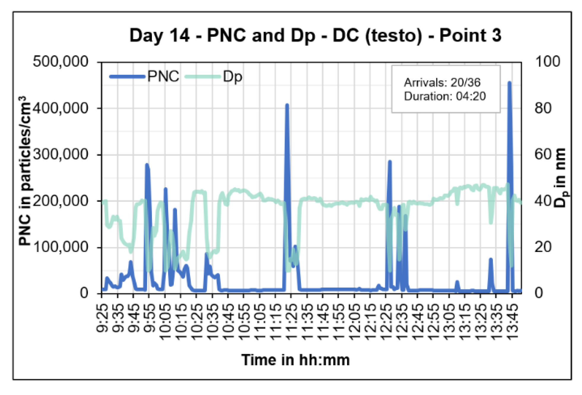
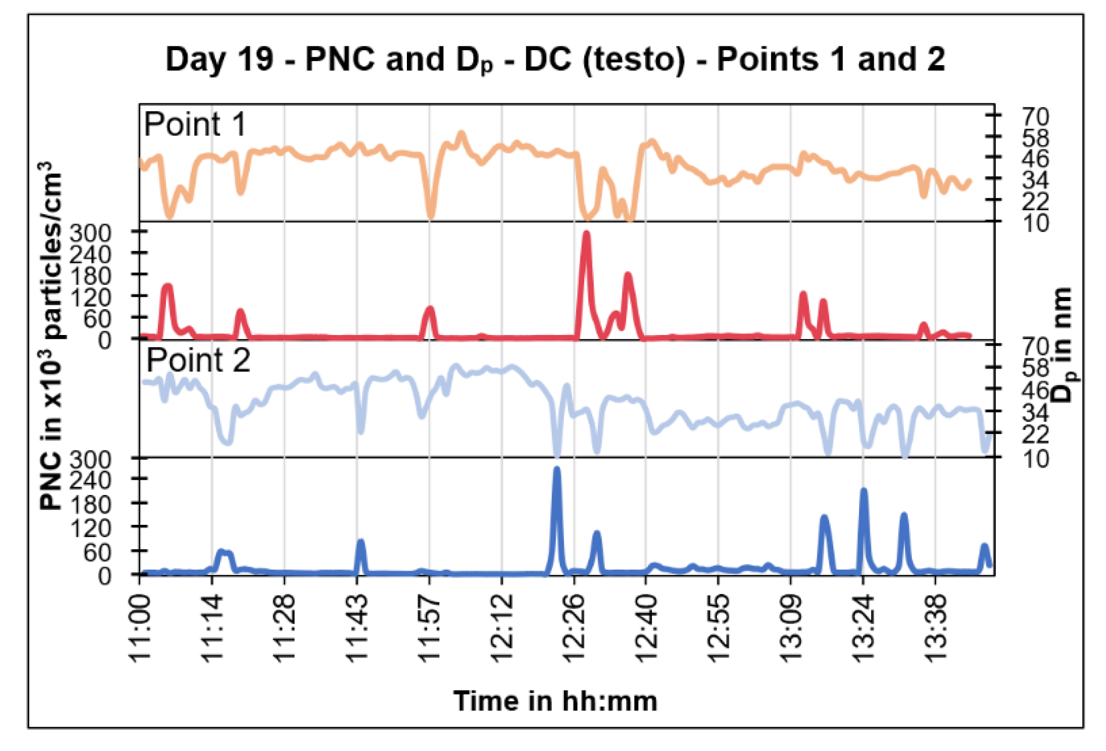
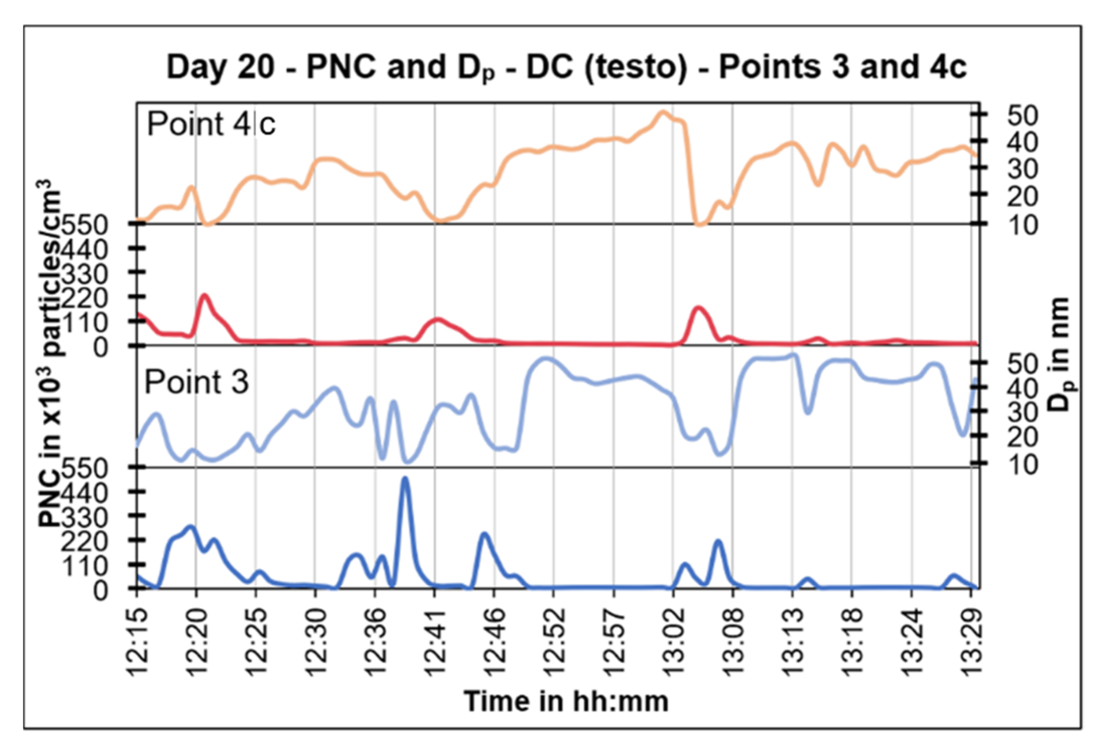
3.1.1. Particle Number Concentrations
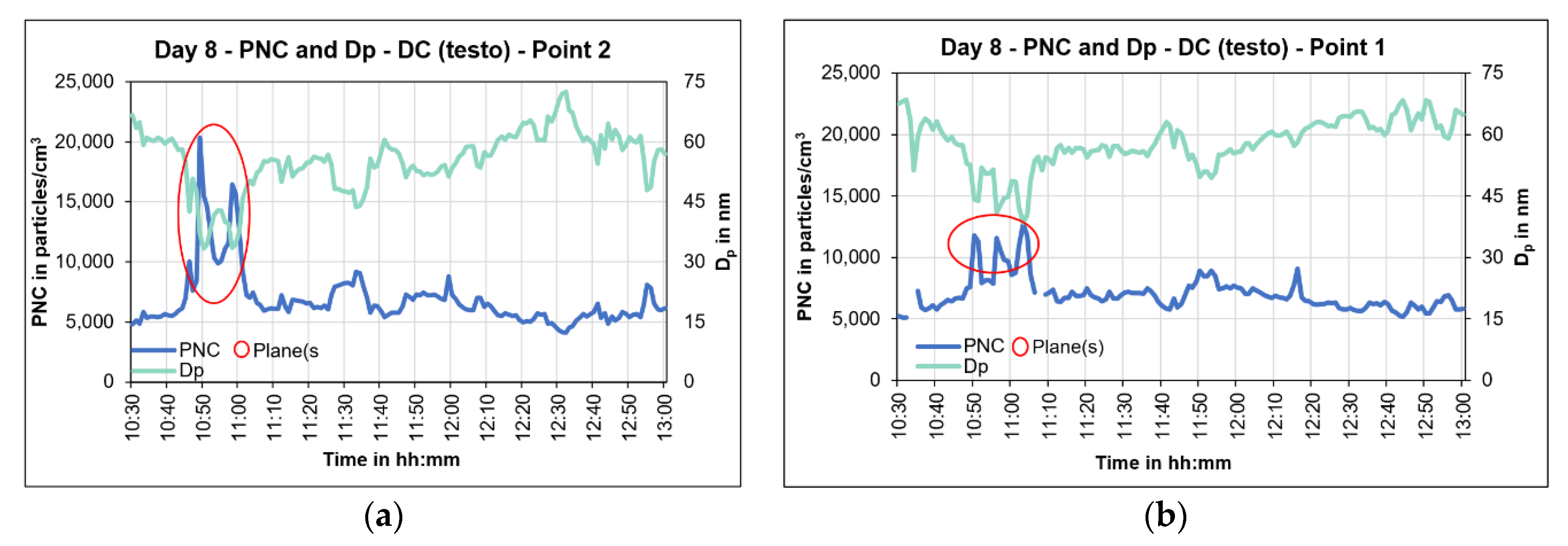
3.1.2. Parallel Measurements
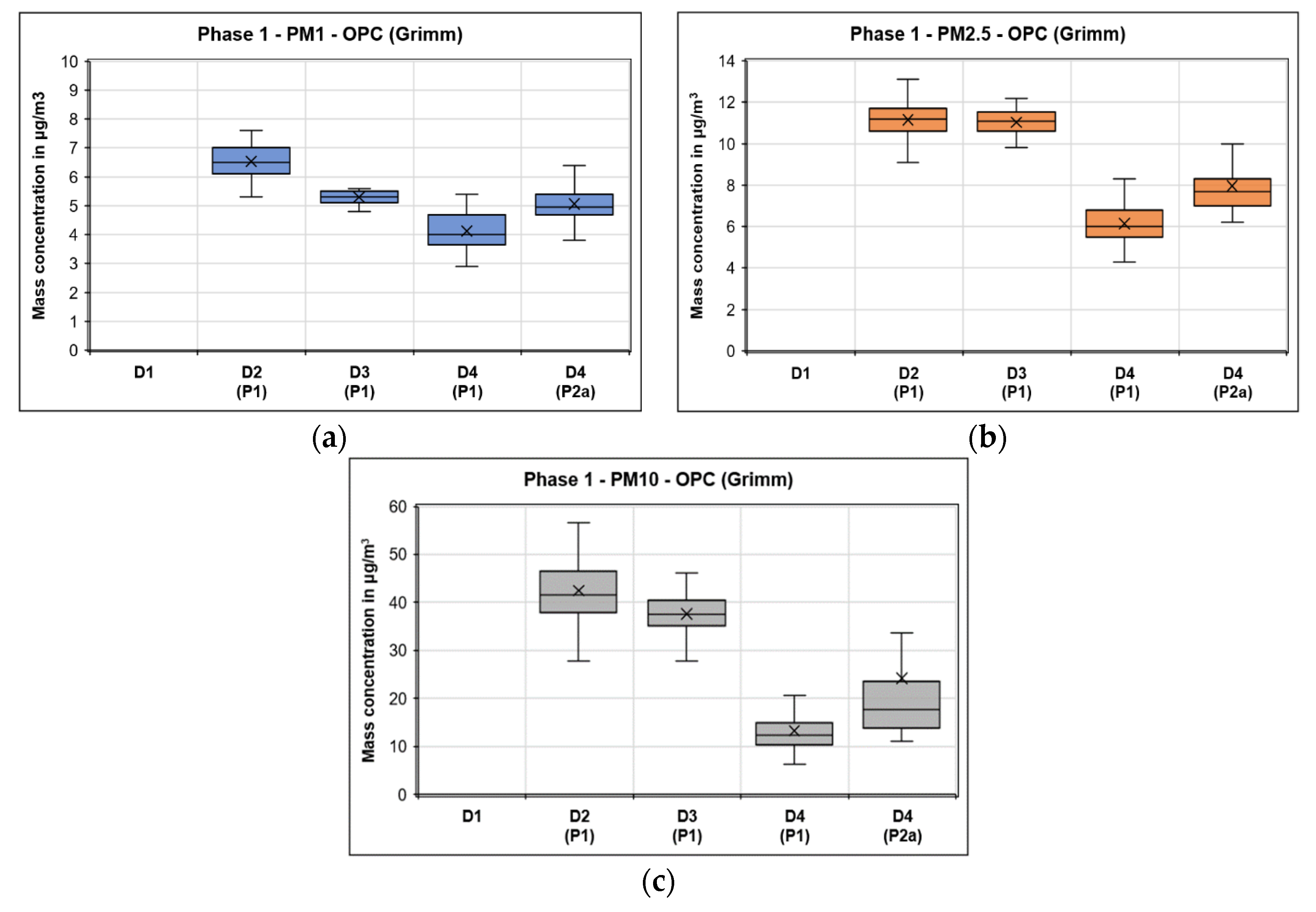
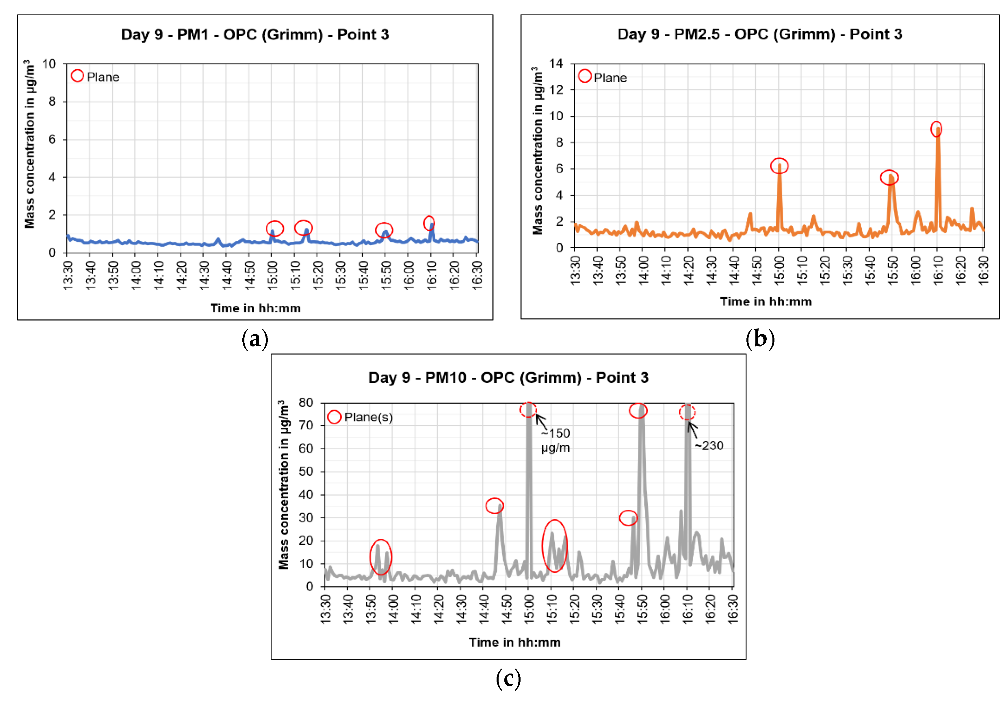
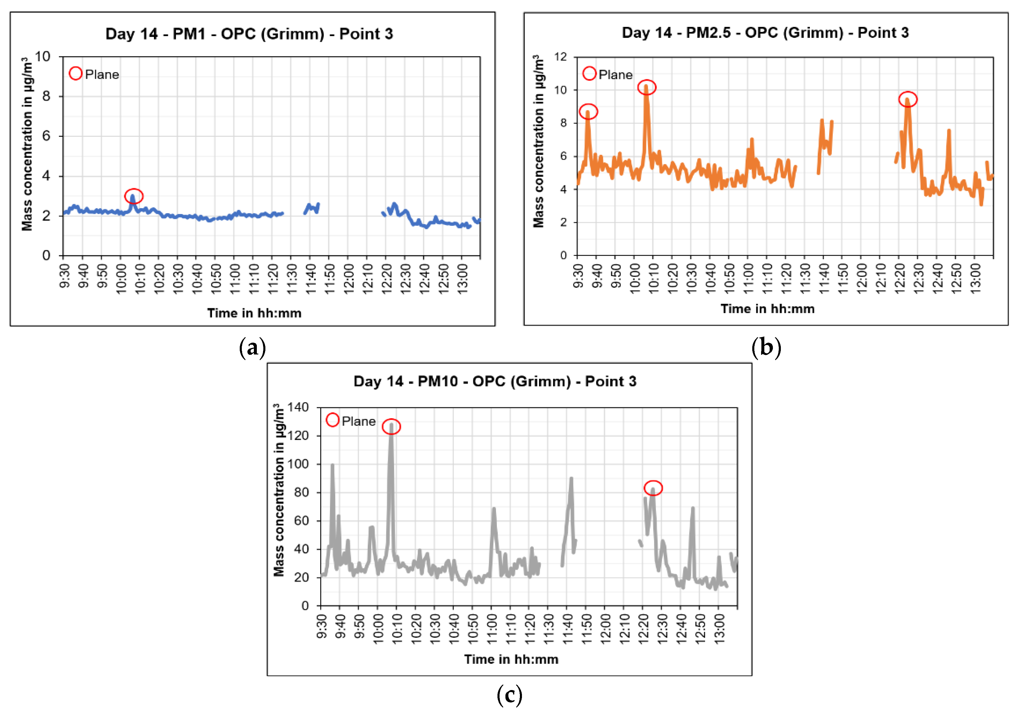
3.1.3. Particle Mass Concentrations
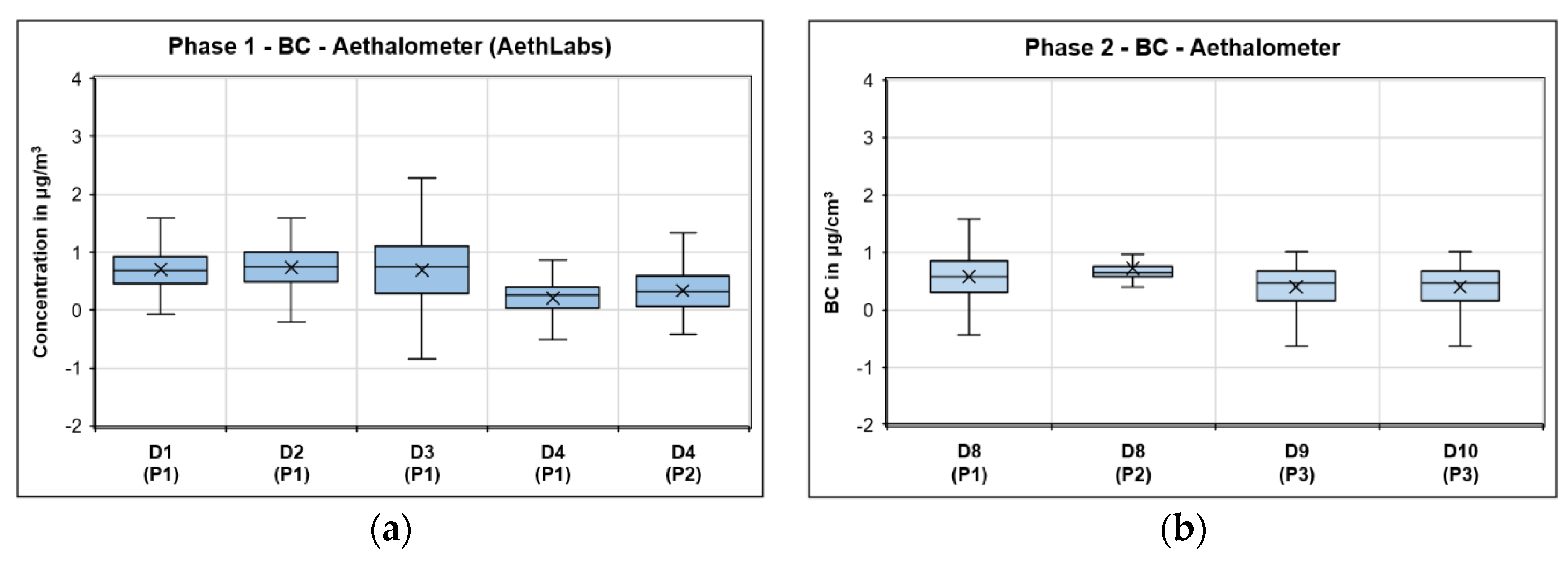
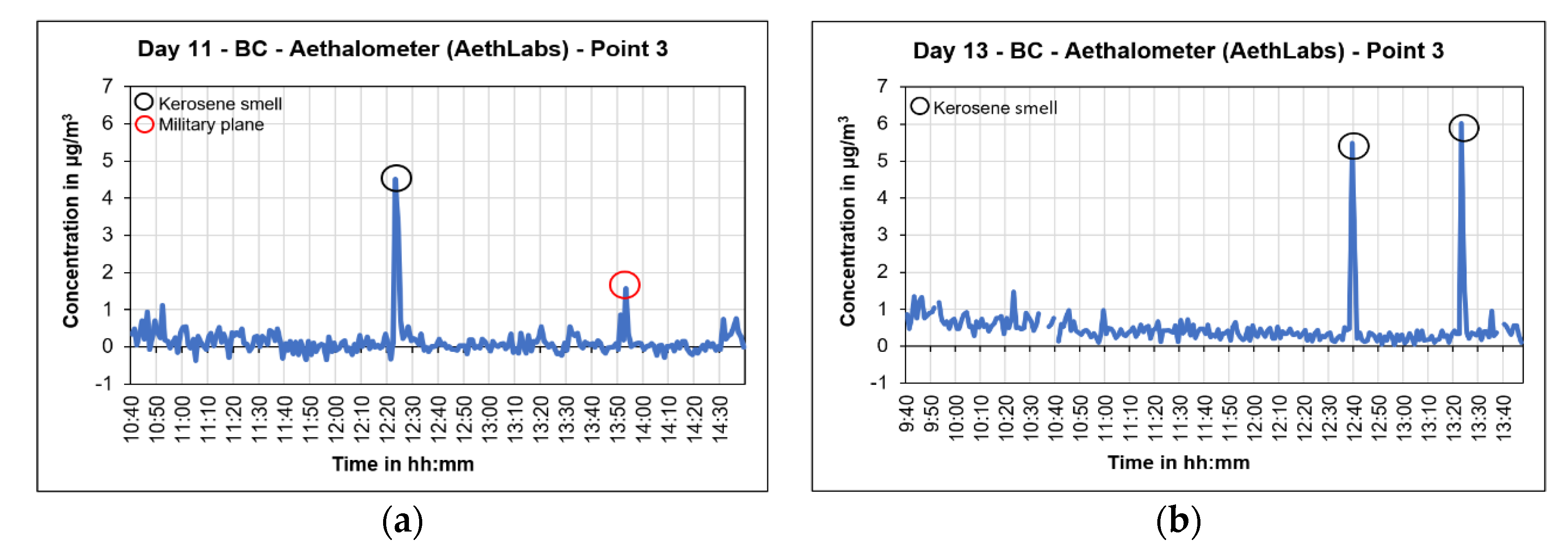
3.1.4. Black Carbon
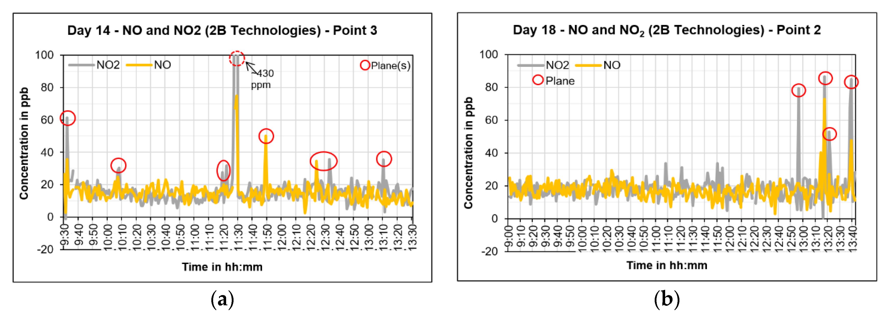
3.1.5. Nitrogen Oxides (NO and NO2)
3.2. Other Sources
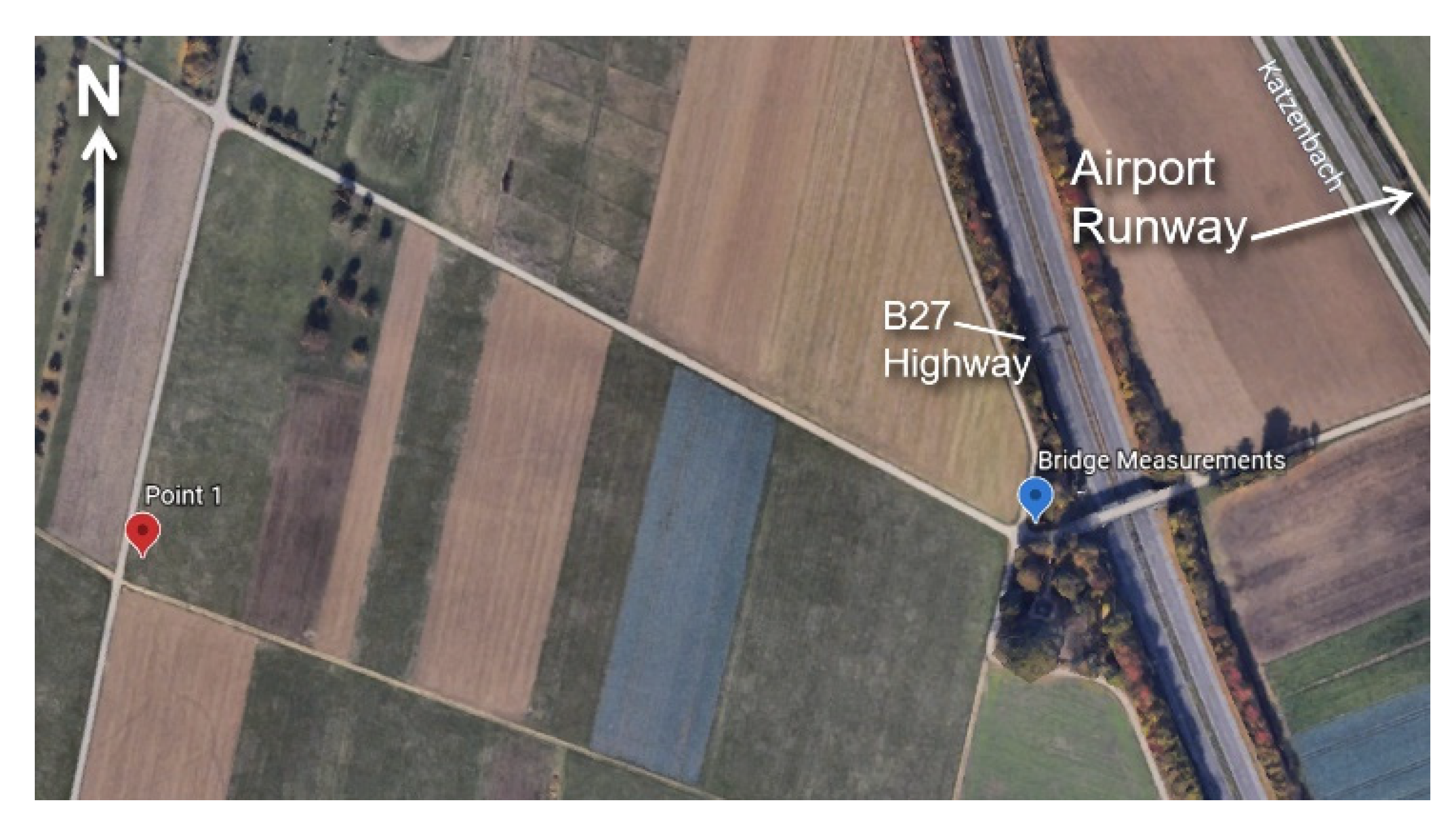
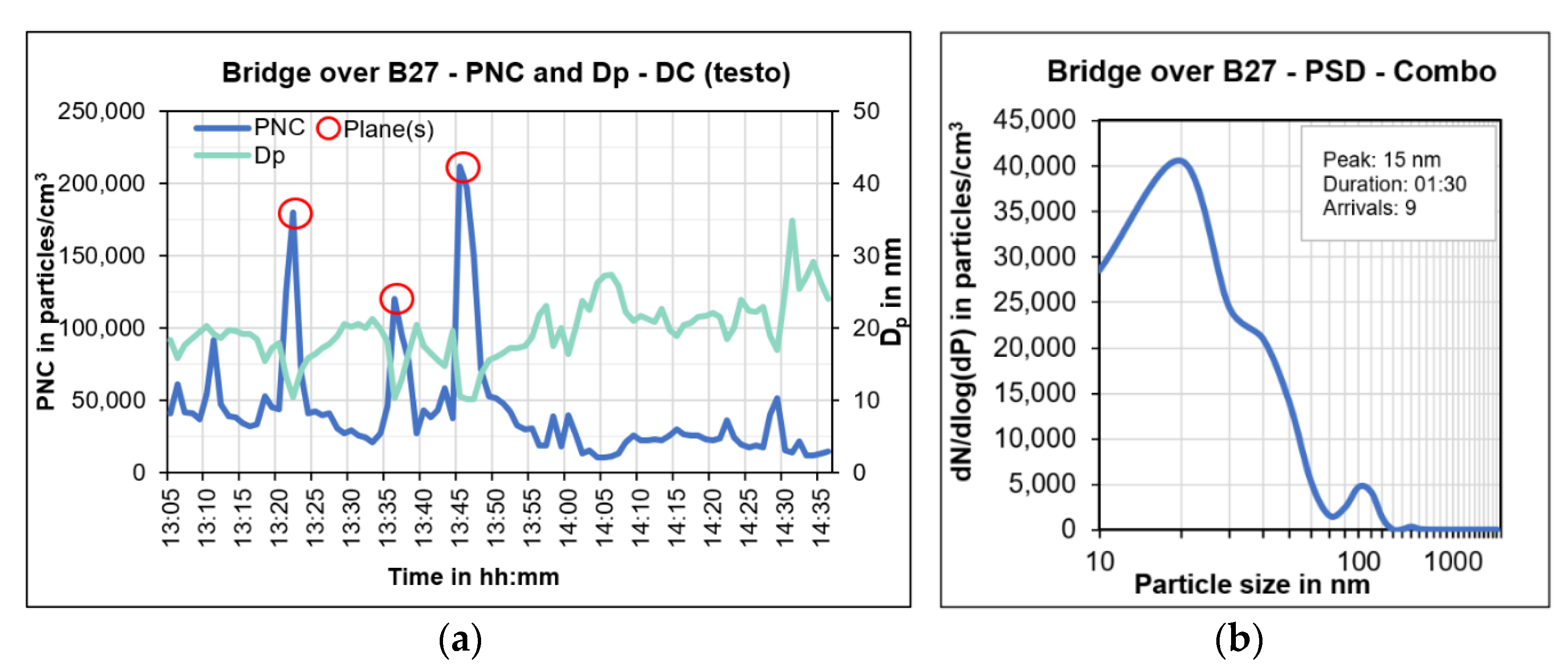
3.2.1. Freeway Measurements
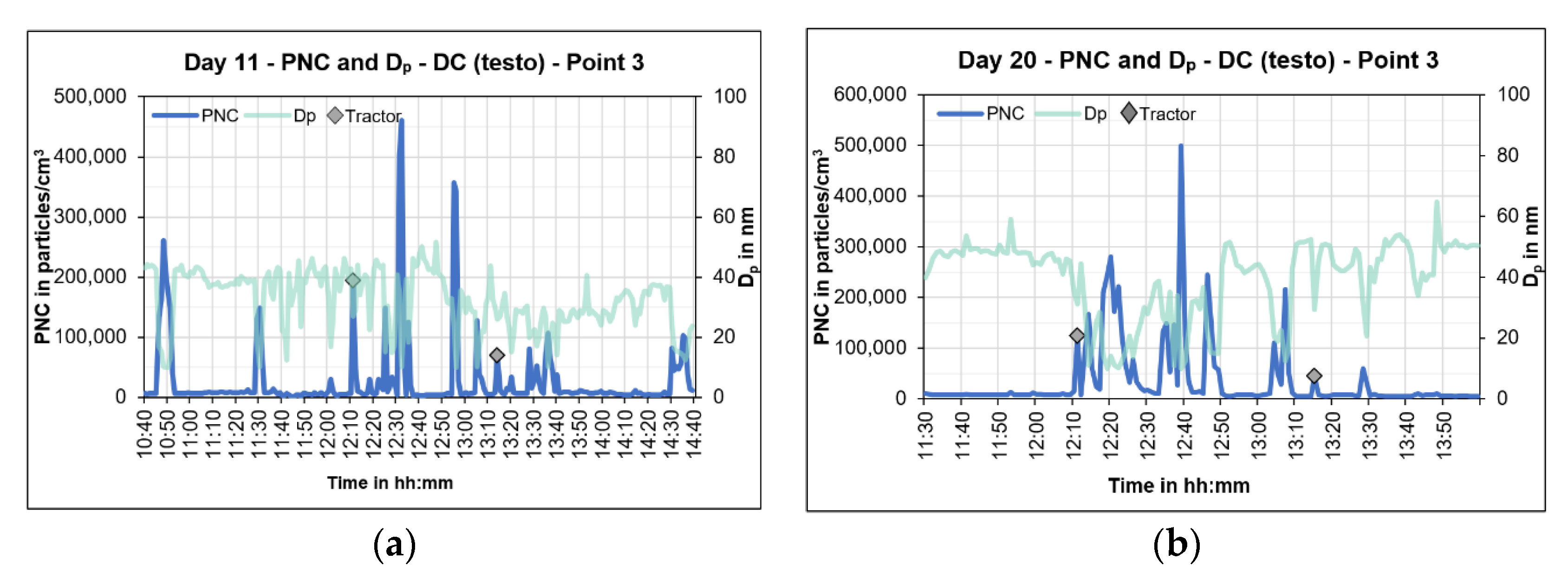
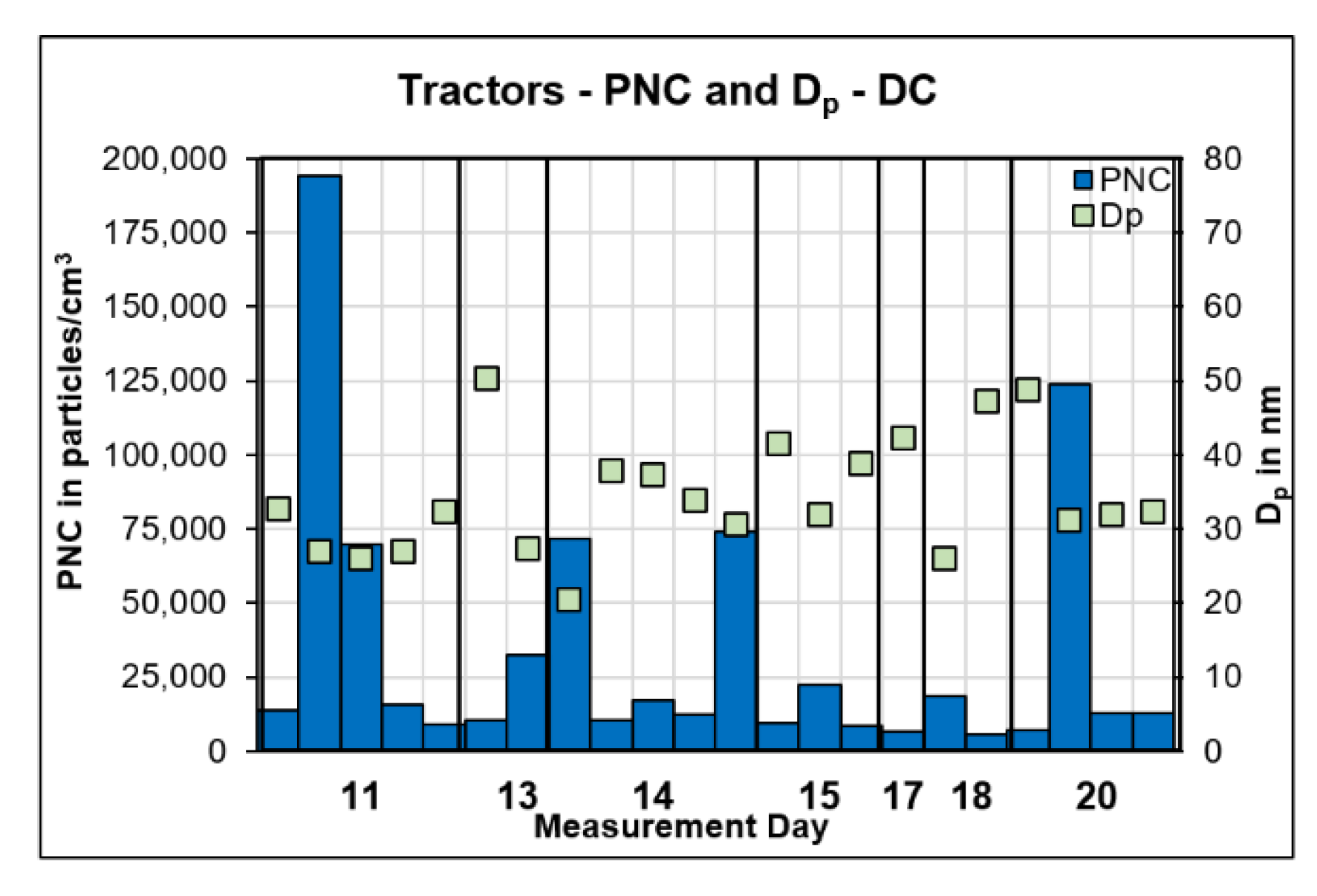
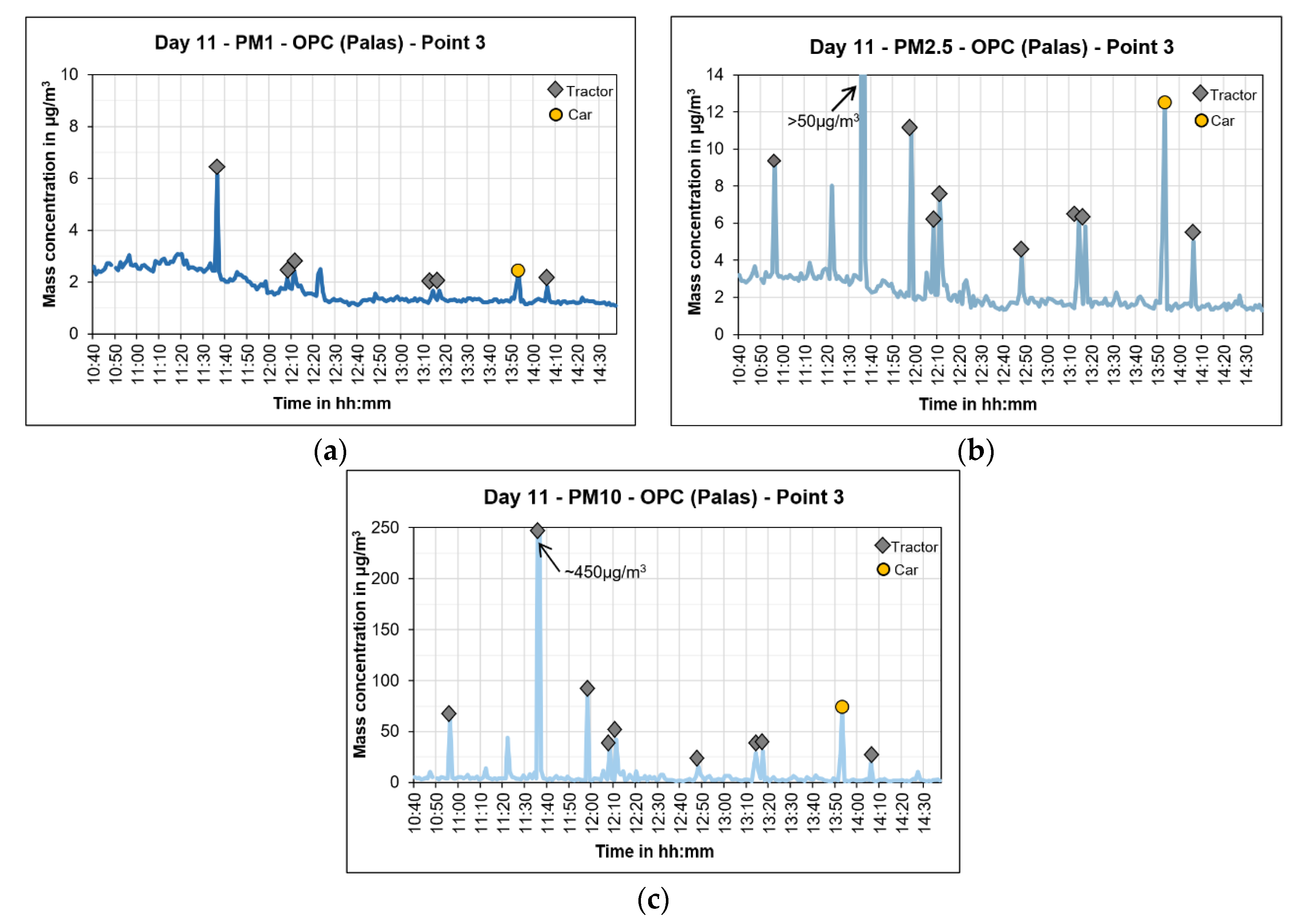
3.2.2. Tractors
3.3. Quality Assurance
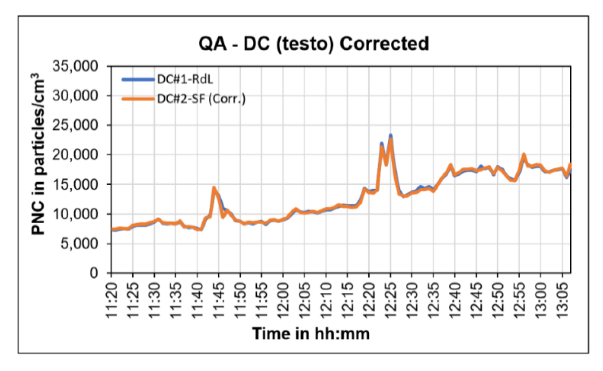
3.3.1. UFP from DC DiSCmini (Testo)
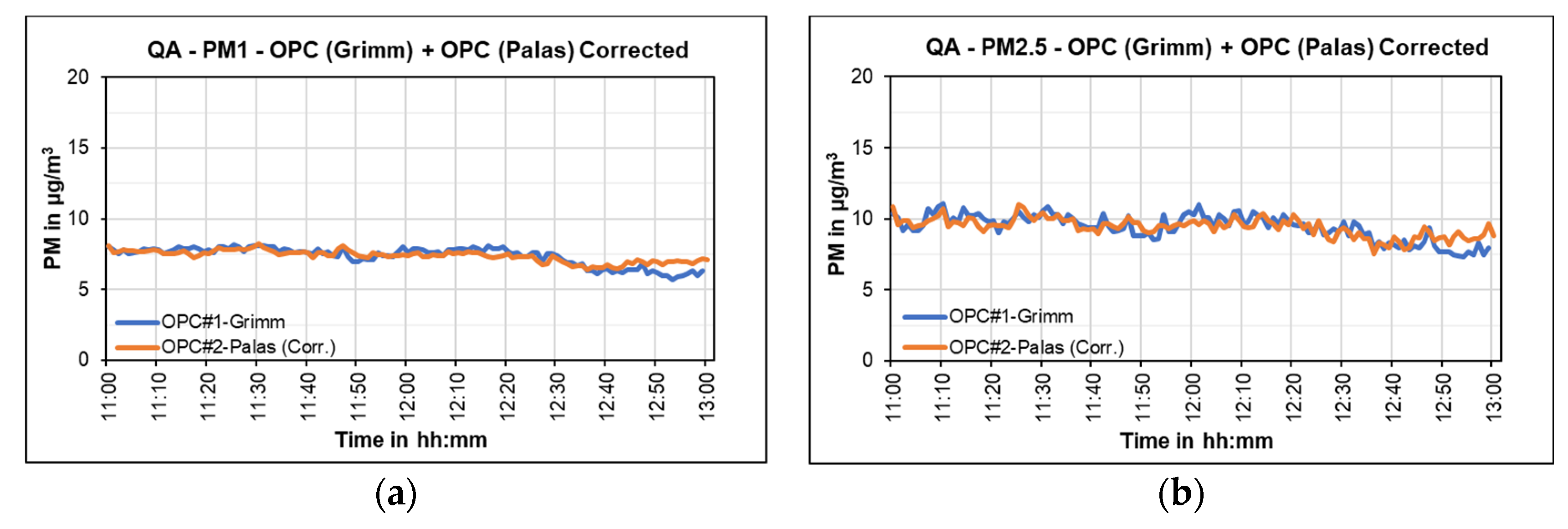
3.3.2. PM from OPC Model 1.108 (Grimm) and OPC Frog (Palas)
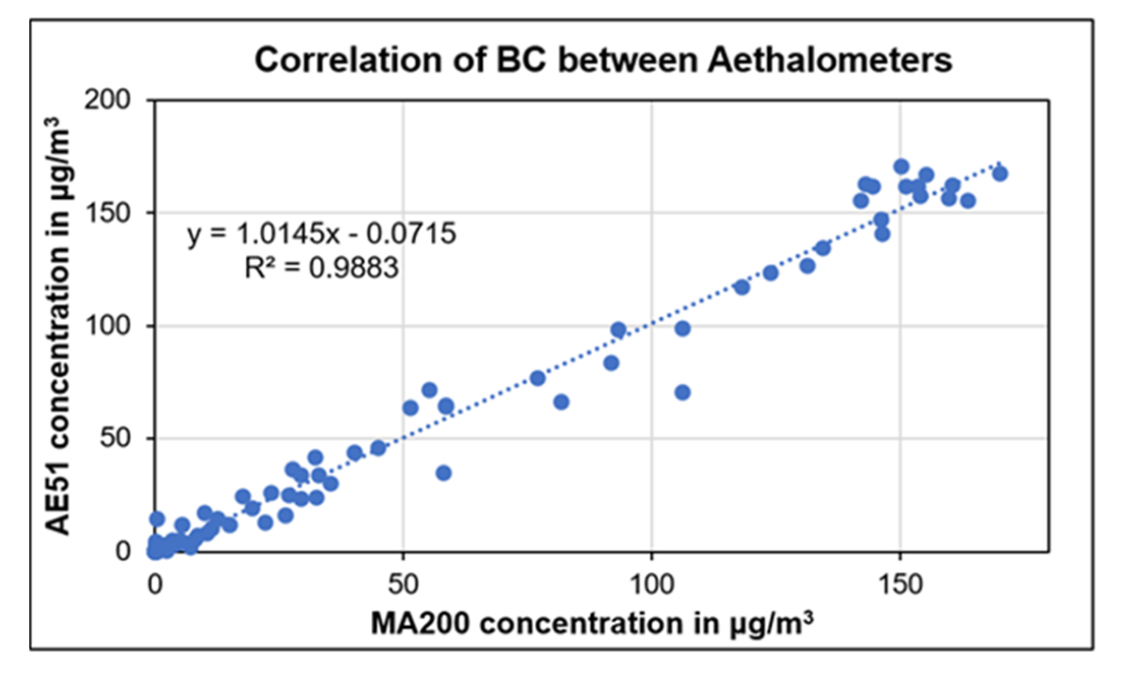
3.3.3. BC Aethalometers from AethLabs
4. Conclusions and Outlook
Author Contributions
Funding
Institutional Review Board Statement
Informed Consent Statement
Data Availability Statement
Conflicts of Interest
References
- Mazareanu, E. Coronavirus: Impact on the Transportation and Logistics Industry Worldwide. Statista. 10 September 2020. Available online: https://www.statista.com/topics/6350/coronavirus-impact-on-the-transportation-and-logistics-industry-worldwide (accessed on 25 September 2022).
- Flughafen Stuttgart GmbH. In Bewegung—Berecht 2018. Inklusive Aktualisierter Umwelterklärung. 2018. Available online: https://www.flughafen-stuttgart.de/media/306484/stuttgart_airport_bericht_2018.pdf (accessed on 22 June 2022).
- Gössling, S.; Hanna, P.; Higham, J.; Cohen, S.; Hopkins, D. Can we fly less? Evaluating the ‘necessity’ of air travel. J. Air Transp. Manag. 2019, 81, 101722. [Google Scholar] [CrossRef]
- Sullivan, A. To Fly or Not to Fly? The Environmental Cost of Air Travel. DW. 2020. Available online: https://www.dw.com/en/to-fly-or-not-to-fly-the-environmental-cost-of-air-travel/a-42090155 (accessed on 24 January 2022).
- Westerdahl, D.; Fruin, S.A.; Fine, P.L.; Sioutas, C. The Los Angeles International Airport as a source of ultrafine particles and other pollutants to nearby communities. Atmos. Environ. 2008, 42, 3143–3155. [Google Scholar] [CrossRef]
- Hudda, N.; Gould, T.; Hartin, K.; Larson, T.V.; Fruin, S.A. Emissions from an international airport increase particle number concentrations 4-fold at 10 km downwind. Environ. Sci. Technol. 2014, 48, 6628–6635. [Google Scholar] [CrossRef] [PubMed]
- Keuken, M.P.; Moerman, M.; Zandveld, P.; Henzing, J.S.; Hoek, G. Total and size-resolved particle number and black carbon concentrations in urban areas near Schiphol airport (the Netherlands). Atmos. Environ. 2015, 104, 132–142. [Google Scholar] [CrossRef]
- Weber, K.; Pohl, T.; Böhlke, C.; Fischer, C.; Kramer, T. Investigation of UFP-Distributions with Stationary and Mobile Measurements at the Düsseldorf Airport. In Proceedings of the 7th International Symposium on Ultrafine Particles, Air Quality and Climate. Institut für Meteorologie und Klimaforschung—Atmosphärische Aerosolforschung (IMK-AAF), Brüssel, Belgien, 15–16 May 2019; Available online: https://publikationen.bibliothek.kit.edu/1000096845 (accessed on 7 August 2020).
- EASA—European Union Aviation Safety Agency. Overview of Aviation Sector. Emissions. With assistance of EEA and EUROCONTROL. 2019. Available online: https://www.easa.europa.eu/eaer/topics/overview-aviation-sector (accessed on 24 June 2022).
- Penman, J. Good Practice Guidance and Uncertainty Management in National Greenhouse Gas Inventories; Institute for Global Environmental Strategies (IGES): Kanagawa, Japan, 2000. [Google Scholar]
- Liu, H.-Y.; Dunea, D.; Iordache, S.; Pohoata, A. A Review of Airborne Particulate Matter Effects on Young Children’s Respiratory Symptoms and Diseases. Atmosphere 2018, 9, 150. [Google Scholar] [CrossRef]
- Raaschou-Nielsen, O.; Andersen, Z.J.; Beelen, R.; Samoli, E.; Stafoggia, M.; Weinmayr, G.; Hoffmann, B.; Fischer, P.; Nieuwenhuijsen, M.J.; Brunekreef, B.; et al. Air pollution and lung cancer incidence in 17 European cohorts: Prospective analyses from the European Study of Cohorts for Air Pollution Effects (ESCAPE). Lancet Oncol. 2013, 14, 813–822. [Google Scholar] [CrossRef] [PubMed]
- Raaschou-Nielsen, O.; Beelen, R.; Wang, M.; Hoek, G.; Andersen, Z.J.; Hoffmann, B.; Stafoggia, M.; Samoli, E.; Weinmayr, G.; Dimakopoulou, K.; et al. Particulate matter air pollution compo-nents and risk for lung cancer. Environ. Int. 2016, 87, 66–73. [Google Scholar] [CrossRef] [PubMed]
- Bentayeb, M.; Wagner, V.; Stempfelet, M.; Zins, M.; Goldberg, M.; Pascal, M.; Larrieu, S.; Beaudeau, P.; Cassadou, S.; Eilstein, D.; et al. Association be-tween long-term exposure to air pollution and mortality in France: A 25-year follow-up study. Environ. Int. 2015, 85, 5–14. [Google Scholar] [CrossRef]
- Ohlwein, S.; Kappeler, R.; On behalf of the German Environmental Agency and the Swiss Federal Office for the Environment. Health Effects of Ultrafine Particles. UMWELT & GESUNDHEIT. 2018. Available online: https://www.umweltbundesamt.de/sites/default/files/medien/376/publikationen/uba_ufp_health_effects_haupt_final.pdf (accessed on 20 July 2022).
- Kumar, P.; Morawska, L.; Birmili, W.; Paasonen, P.; Hu, M.; Kulmala, M.; Harrison, R.M.; Norford, L.; Britter, R. Ultrafine particles in cities. Environ. Int. 2014, 66, 1–10. [Google Scholar] [CrossRef]
- Flughafenverband ADV. Arbeitsgemeinschaft Deutscher Verkehrsflughäfen-Monatsstatistik. 2019. Available online: https://www.adv.aero/service/downloadbibliothek (accessed on 20 July 2022).
- Baumüller, J. (Ed.) Klimaatlas Region Stuttgart—Stadtklima 21: Grundlagen zum Stadtklima und zur Planung. 2018, p. 28. Available online: https://www.stadtklima-stuttgart.de/index.php?klima_klimaatlas_region (accessed on 20 July 2022).
- Stuttgart Airport. The Project. Stuttgart Flughafen GmbH. 2020. Available online: https://www.stuttgart-airport.com/company-information/runway-renewal/the-project/ (accessed on 4 September 2022).
- Schröder, D. Verheerender Waldbrand: Feuerwehr Löscht Weiter Glutnester—Mann Macht Geständnis. WA Medien Gruppe. 2020. Available online: https://www.wa.de/nordrhein-westfalen/gummersbach-grosser-waldbrand-feuerwehr-polizei-gestaendnis-13668308.html (accessed on 8 May 2020).
- TSI Incorporated. Nanoscan SMPS Nanoparticle Sizer Model 3910. 2012. Available online: https://tsi.com/getmedia/3188cb1d-2362-44c0-82b4-f2cc60afef17/NanoScan%20SMPS%203910_5001411?ext=.pdf (accessed on 1 September 2022).
- TSI Incorporated. Hand-Held Condensation Particle Counter Model 3007. 2022. Available online: https://www.tsi.com/getmedia/8c0677b4-6cda-43b6-9a74-1c96acc30d4e/3007_5001117_A4?ext=.pdf (accessed on 1 September 2022).
- Palas GmbH. Fine Dust Measuring Device Operating Manual—Fidas Frog. 2017. Available online: https://www.manualslib.com/manual/2052143/Palas-Fidas-Frog.html (accessed on 1 September 2022).
- TSI Incorporated. Model 3330 Optical Particle Sizer Spectrometer Manual. 2013. Available online: https://www.kenelec.com.au/wp-content/uploads/2016/06/TSI_3330_Opticle_Particle_Sizer_Manual.pdf (accessed on 1 September 2022).
- Grimm Aerosol Technik GmbH & Co. KG. Portable Laser Aerosolspectrometer and Dust Monitor Model 1.108/1.109. 2010. Available online: https://cires1.colorado.edu/jimenez-group/Manuals/Grimm_OPC_Manual.pdf (accessed on 1 September 2022).
- Testo DISCmini. Diffusion Size Classifier Miniature. 2016. Available online: https://static-int.testo.com/media/ae/87/df0045b6f8dd/pb-testo-DiSCmini-Brochure-US.pdf (accessed on 1 September 2022).
- AethLabs. microAeth AE51 Operating Manual. Rev 06 Updated July 2016. Available online: https://aethlabs.com/sites/all/content/microaeth/ae51/microAeth%20AE51%20Operating%20Manual%20Rev%2006%20Updated%20Jul%202016.pdf (accessed on 1 September 2022).
- AethLabs. MA200 MA300 MA350 Operating Manual. Rev 03 December 2018. Available online: https://aethlabs.com/sites/all/content/microaeth/maX/MA200%20MA300%20MA350%20Operating%20Manual%20Rev%2003%20Dec%202018.pdf (accessed on 1 September 2022).
- LI-COR, Inc. Using the LI-830 and LI-850 Gas Analyzers. 2022. Available online: https://www.licor.com/documents/gz8gaf0ls5vhvpl52xtmyr8mfoh5kwe8 (accessed on 1 September 2022).
- 2B Technologies, Inc. NO2/NO/NOX Monitor Operation Manual Model 405 nm. 2018. Available online: https://twobtech.com/docs/manuals/model_405nm_revG-5.pdf (accessed on 1 September 2022).
- 2B Technologies, Inc. Ozone Monitor Operation Manual Model 202. 2018. Available online: https://twobtech.com/docs/manuals/model_202_revJ-4.pdf (accessed on 1 September 2022).
- GILL Instruments Limited. MaxiMet-Manual-Iss-6. Compact Weather Stations. 2017. Available online: https://gillinstruments.com/wp-content/uploads/2022/08/1957-009-Maximet-gmx501-Iss-9.pdf (accessed on 1 September 2022).
- Vorage, M.; Madl, P.; Hubmer, A.; Lettner, H. Aerosols at Salzburg Airport: Long-term measurements of ultrafine particles at two locations along the runway. Gefahrst. Reinhalt. Luft 2019, 79, 227–234. [Google Scholar] [CrossRef]
- Lammers, A.; Janssen, N.A.H.; Boere, A.J.F.; Berger, M.; Longo, C.; Vijverberg, S.J.H.; Neerincx, A.H.; van der Zee, A.H.M.; Cassee, F.C. Effects of short-term exposures to ultrafine particles near an airport in healthy subjects. Environ. Int. 2020, 141, 105779. [Google Scholar] [CrossRef]


| Date | Weekday | Measurement Day | Point | Time |
|---|---|---|---|---|
| Phase 1 | ||||
| 16 April 2020 | Thursday | 1 | P1 | 15:15 |
| 17 April 2020 | Friday | 2 | P1 | 14:45 |
| 18 April 2020 | Saturday | 3 | P1 | 14:40 |
| 19 April 2020 | Sunday | 4 | P1 | 13:40 |
| P2 | 13:05 | |||
| 20 April 2020 | Monday | 5 | P1 | 13:05 |
| P2 | 13:45 | |||
| 21 April 2020 | Tuesday | 6 | P1 | 14:10 |
| 22 April 2020 | Wednesday | 7 | P1 | 14:55 |
| 23 April 2020 | Thursday | QA | P1 | 14:00 |
| Phase 2 | ||||
| 3 June 2020 | Wednesday | 8 | P1 | 14:35 |
| P2 | 13:00 | |||
| 18 June 2020 | Thursday | 9 | P3 | 15:00 |
| 19 June 2020 | Friday | 10 | P3 | 14:00 |
| Phase 3 | ||||
| 19 August 2020 | Wednesday | 11 | P3 | 16:00 |
| 20 August 2020 | Thursday | 12 | P1 | 14:45 |
| P4b | 14:00 | |||
| 21 August 2020 | Friday | 13 | P3 | 16:00 |
| P4b | 16:00 | |||
| 25 August 2020 | Tuesday | 14 | P3 | 16:00 |
| 27 August 2020 | Thursday | 15 | P4b | 14:50 |
| P1 | 13:00 | |||
| P4b | 13:30 | |||
| P2 | 12:50 | |||
| 3 September 2020 | Thursday | 16 | P4b | 14:50 |
| P3 | 14:50 | |||
| 4 September 2020 | Friday | 17 | P3 | 15:00 |
| P4b/c | 14:00 | |||
| 7 September 2020 | Monday | 18 | P2 | 17:00 |
| P1 | 14:30 | |||
| 8 September 2020 | Thursday | 19 | P2 | 14:30 |
| P1 | 14:20 | |||
| 9 September 2020 | Wednesday | 20 | P3 | 14:20 |
| P4c | 14:00 | |||
| Parameter | Measurement Technique and Principle | Equipment Model | Measurement Range | Phase |
|---|---|---|---|---|
| UFP + size distribution | Scanning Mobility Particle Sizer (SMPS) + Condensation Particle Counter (CPC) → Particle condensation | NanoScan 3910 (TSI) | 10–420 nm | 1, 2, 3 |
| UFP | Diffusion charger (DC) × 2 | DiSCmini (testo) | 10–700 nm | 1, 2, 3 |
| UFP | Condensation Particle Counter (CPC) | Model 3007 (TSI) | 10–1000 nm | 1, 2, 3 |
| PM2.5, PM10 + size distribution | Optical Particle Counter (OPC) → Light scattering | OPS 3330 (TSI) | 0.3–10 µm | 1, 2, 3 |
| PM2.5, PM10 + size distribution | Optical Particle Counter (OPC) → Light scattering | Fidas Frog (Palas) | 0.15–18 µm | 1, 2, 3 |
| PM2.5, PM10 + size distribution | Optical Particle Counter (OPC) → Light scattering | Model 1.108 (Grimm) | 0.3–20 µm | 1, 2, 3 |
| BC | Aethalometry → IR and visible light absorption | MA200 (AethLabs) | 0–1 mg BC/m3 | 1, 2, 3 |
| BC | Aethalometry → IR light absorption | AE51 (AethLabs) | 0–1 mg BC/m3 | 1, 2, 3 |
| CO2 | IR absorption | LI-830 (LI-COR) | 0–20,000 ppm | 2, 3 |
| NO2 NO | Light absorption (405 nm) | NO/NO2/NOX monitor 405 nm (2B technologies) | 0–10 ppm 0–2 ppm | 2, 3 |
| O3 | UV absorption (254 nm) | Ozone monitor 202 (2B technologies) | 3 ppb–250 ppm | 2, 3 |
| Wind speed + direction | Compact weather station | MaxiMet GMX501 (Gill) | - | 1, 2, 3 |
| Characteristics | Phase 1 | Phase 2 | Phase 3 |
|---|---|---|---|
| Number of flights | No flight activity | Six flights/hour on average | Ten flights/hour on average |
| Meteorological conditions | Primarily NE direction, low wind speed, clear weather/no rain | N and S winds, low wind speeds, rain between measurement days | Varying wind direction, low wind speeds, rain between measurement days |
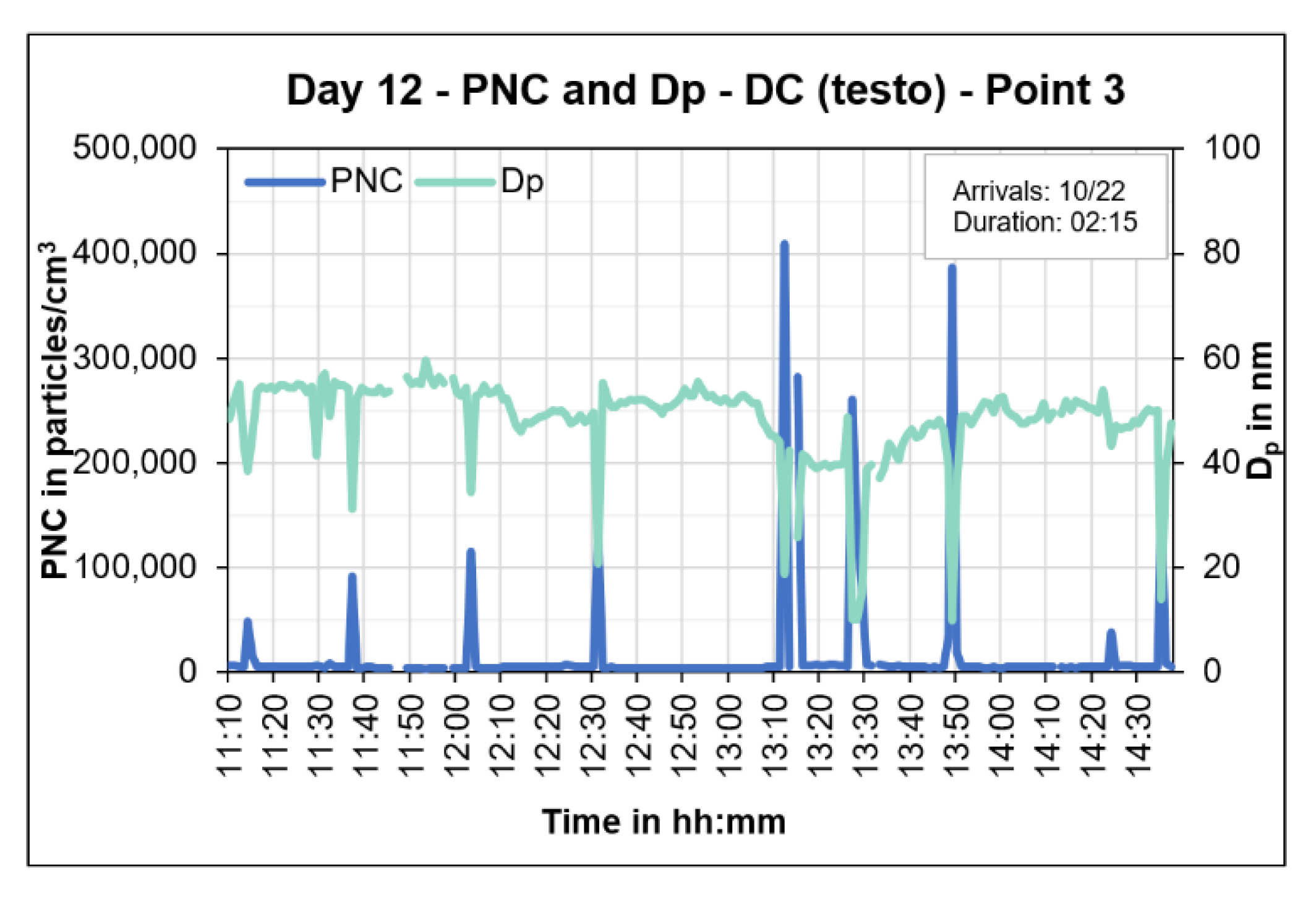
| PNC | <10,000 particles/cm3 with little variation | Peaks ranged from 20,000 to 40,000 particles/cm3 | Peaks ranged from 30,000 to 800,000 particles/cm3 |
| PM | PM1 and PM2.5 values were low. PM2.5 and PM10 under limit values | PM1 and PM2.5 values still low. PM2.5 within limit values. Several PM10 peaks > 50 µg/m3 from flights | PM concentrations slightly higher than Phase 2. PM2.5 within limit values. Several PM10 peaks > 50 µg/m3 from flights |
| Dp, second percentile | 38 to 65 nm | 21 to 42 nm | 10 to 22 nm |
| PSD peak | Between 27 nm and 86 nm | Between 27 nm and 36 nm | 10 nm |
| BC | <1 µg/m3 Minimal changes and variation | <1 µg/m3 Minimal changes and variation | Several BC peaks > 1 µg/m3 from aircraft related activity |
| Gas monitors | Not used | CO2: 433 ppm NO2: 9 ppb NO: - O3: 71 ppb | CO2: 400 ppm NO2: 16 ppb NO: 11 ppb O3: 50 ppb |
Publisher’s Note: MDPI stays neutral with regard to jurisdictional claims in published maps and institutional affiliations. |
© 2022 by the authors. Licensee MDPI, Basel, Switzerland. This article is an open access article distributed under the terms and conditions of the Creative Commons Attribution (CC BY) license (https://creativecommons.org/licenses/by/4.0/).
Share and Cite
Samad, A.; Arango, K.; Chourdakis, I.; Vogt, U. Contribution of Airplane Engine Emissions on the Local Air Quality around Stuttgart Airport during and after COVID-19 Lockdown Measures. Atmosphere 2022, 13, 2062. https://doi.org/10.3390/atmos13122062
Samad A, Arango K, Chourdakis I, Vogt U. Contribution of Airplane Engine Emissions on the Local Air Quality around Stuttgart Airport during and after COVID-19 Lockdown Measures. Atmosphere. 2022; 13(12):2062. https://doi.org/10.3390/atmos13122062
Chicago/Turabian StyleSamad, Abdul, Kathryn Arango, Ioannis Chourdakis, and Ulrich Vogt. 2022. "Contribution of Airplane Engine Emissions on the Local Air Quality around Stuttgart Airport during and after COVID-19 Lockdown Measures" Atmosphere 13, no. 12: 2062. https://doi.org/10.3390/atmos13122062
APA StyleSamad, A., Arango, K., Chourdakis, I., & Vogt, U. (2022). Contribution of Airplane Engine Emissions on the Local Air Quality around Stuttgart Airport during and after COVID-19 Lockdown Measures. Atmosphere, 13(12), 2062. https://doi.org/10.3390/atmos13122062