Abstract
On 15 January 2022, the Hunga Tonga-Hunga Ha’apai (HTHH) (175.38° W, 20.54° S) volcano erupted explosively. It is considered the most explosive volcanic eruption during the past 140 years. The HTHH volcanic eruption caused intense ripples, Lamb waves, and gravity waves in the atmosphere which encircled the globe several times, as reported by different studies. In this study, using OMI, SAGE-III/ISS, and CALIPSO satellite observations, we investigated the spread of the volcanic SO2 cloud due to the HTHH eruption and subsequent formation of sulfuric acid clouds in the stratosphere. It took about 19–21 days for the stratospheric SO2 injections of the HTHH to encircle the globe longitudinally due to a dominant westward jet with wind speeds of ~2500 km/day, and it slowly dispersed over the whole globe within several months due to poleward spread. The formation of sulfuric acid clouds intensified after about a month, causing the more frequent occurrence of high aerosol optical depth elevated layers in the stratosphere at an altitude of about 20–26 km. This study deals with the dynamics of volcanic plume spread in the stratosphere, knowledge of which is essential in estimating the accurate radiative effects caused by perturbations in the earth–atmosphere system due to a volcanic eruption. In addition, this knowledge provides important input for studies related to the geo-engineering of the earth’s atmosphere by injecting particulates and gases into the stratosphere.
1. Introduction
Vast amounts of gases and aerosol particles injected into the stratosphere due to volcanic eruptions result in the perturbation of the radiative balance of the earth and the chemical equilibrium of the stratosphere. Substantial increases in stratospheric aerosols from volcanic eruptions are considered as natural climate experiments as they provide an opportunity to examine the effects on the climate resulting from abrupt perturbations in the atmosphere [1,2,3].
There are a number of well-known processes that ensue gradually in the stratosphere succeeding a volcanic eruption. Strong volcanic eruptions directly inject large amounts of sulfur dioxide (SO2), carbon dioxide (CO2) [4,5,6], water vapor [7], and other trace gases into the stratosphere. The directly injected volcanic emissions disperse and cover the global stratosphere rapidly over a typical time period of about 20 days to 1 month [3,8,9,10].
In contrast to their much shorter lifetimes in the troposphere, the volcanic SO2 clouds in the stratosphere are converted to sulfuric acid (H2SO4) clouds consisting of tiny sulfate aerosol particles in the presence of hydroxyl (OH) radicals (due to oxidation), and the subsequent transformation leads to an increase in the total amount of stratospheric aerosol [11]. This increases the optical depth, causing an enhancement in scattering and absorption of solar radiation, resulting in an increase in albedo and a net loss of energy [3]. Winds rapidly disperse the particles throughout the lower stratosphere. Because of the typical 1–2-year residence time of the particles in the stratosphere, stratospheric aerosol injections become nearly global in extent, resulting in near-global perturbation to the radiative energy balance.
Volcanic eruptions inject large amounts of particles into the lower stratosphere. This causes the radiative heating of the stratosphere and the cooling of the surface/troposphere. The stratosphere gains shortwave radiative energy while the surface experiences a deficit due to the volcanic aerosol layer. Because of the dominant scattering of the solar radiation by the sulfate aerosols, the net effect of volcanic eruptions is to cool the planet [1,3]. Following radiative balance perturbations there are multiple complex feedback processes affecting the entire Earth–atmosphere system at different scales [12,13,14]. For example, the perturbation in solar flux due to the Mount Pinatubo volcanic eruption, with a volcanic explosivity index 6, injected approximately 30 Tg of volcanic ash into the stratosphere, was reported to cause an average global cooling of −0.5 °C for ~2 years [15,16].
An increase in the concentration or surface area density of sulfate aerosols provides additional pathways of heterogeneous chemistry and modifies the relative importance of the catalytic processes responsible for ozone depletion in the stratosphere due to changes in ClOx-induced ozone depletion chemistry through the intermediary of NOx chemistry [17]. The increase in stratospheric aerosol surface area resulting from a volcanic eruption also makes these catalytic processes more effective for ozone depletion [18,19].
The increase in stratospheric aerosol optical depth (AOD) causes local heating due to the absorption of solar radiation, which results in changes in thermal structure and mean circulation patterns. A change in mean circulation can affect the vertical distribution of ozone, causing local depletion. A temperature change can change the reaction rate constants for several reactions, causing a change in the production/destruction of ozone. Changes in actinic flux will also affect the photo dissociation rate and affect the ozone balance [18].
Several major eruptions, including Agung in 1963, El Chichón in 1982, and Pinatubo in 1991, occurred during the last century. Investigations of the Mt. Pinatubo eruption provided significant knowledge on the radiative forcing and response characteristics of stratospheric aerosols [20,21]. The eruption of Mount Pinatubo had significant effects on the earth’s climate. Top-of-atmosphere radiation measurements from satellites showed that the Mount Pinatubo eruption resulted in a significant decrease in absorbed solar radiation in the earth–atmosphere system. The global mean decrease in absorbed solar radiation in the period immediately following the eruption was about 5 Wm−2. The albedo of the earth–atmosphere system increased by up to 0.007 because of the reflection of up to an additional 2.5 Wm−2 of solar radiation over the following two years [22,23]. The most optically thick portions of the aerosols from Mt. Pinatubo were located between an altitude of 20 km and 25 km and were confined to 10° S–30° N during the early period [24,25]. The stratospheric aerosol optical depths up to latitudes of at least 70° N were observed to be affected within 2–3 months after the eruption. The global mean stratospheric aerosol optical depth increased by 1400% within the first year following the eruption (from approximately 0.01 to a peak value of 0.14) [22]. The stratospheric aerosol surface area concentrations at mid-latitudes increased by ~40% due to Mt. Pinatubo, and in the core of the volcanic plume they were increased by 70% [26,27].
The Hunga Tonga-Hunga Ha’apai (HTHH) volcano (175.38° W, 20.54° S) erupted explosively at 04:00–04:10 UTC on 15 January 2022. As this was a submarine explosion, it injected a substantial amount of water and ice into the stratosphere [28]. It has been reported that the eruption caused the formation of umbrella clouds at 31 km and at 17 km. The highest plume reached approximately 55–58 km [29,30,31]. A very strong westward propagation of the upper umbrella cloud was observed [30]. Gupta et al. [30] reported on the growth and spread of the umbrella cloud after the eruption based on Himawari satellite data. There are several studies reporting intense Lamb wave and gravity wave activity from the surface to the ionosphere due to the HTHH eruption based on joint satellite observations [32,33,34,35,36,37]. The radiative effects of the HTHH eruption have also been computed [38,39]. The HTHH eruption was reported to cause significant hydration of the stratosphere [40].
In this study, we investigated how the SO2 plume spread globally after the HTHH volcanic eruption, the subsequent formation of the sulfuric acid cloud, and its optical effects, based on multi-satellite observations. This study shows the following: (1) the SO2 plume encircled the globe within 19–21 days of the HTHH eruption, with a mean spread speed of ~2500 km/day. (2) The aerosol concentration was enhanced at an altitude range of 20–25 km due to new particle formation triggered by the increased amount of SO2 and subsequent growth. (3) The peak enhancement in the aerosol extinction coefficient was ~600% of the unperturbed pre-HTHH eruption level. (4) A visualization of the dynamics of the changes in aerosol population. (5) The effects of stratospheric circulation patterns, such as the quasi-biennial oscillation (QBO), Brewer Dobson circulation, and large scale Rossby waves, are clearly shown. (6) A prominent asymmetrical distribution of the sulfuric acid clouds in the southern hemisphere is observed.
2. Data and Methodology
The satellite data listed in Table 1 were used for this study.

Table 1.
List of satellite data products used for this study.
2.1. OMSO2 L2 Dataset from OMI Observations
The Aura Ozone Monitoring Instrument (OMI) level 2 sulfur dioxide (SO2) total column product (OMSO2) [41] data were used for this study. The retrieval was based on a principal component analysis (PCA)-based algorithm with new SO2 Jacobian lookup tables and a priori profiles. Each file contains data from the daylit half of an orbit (~53 min). There are approximately 14 orbits per day. The resolution of the data is 13 × 24 km2 at nadir, with a swath width of 2600 km and 60 pixels per scan line every 2 s.
For each OMI scene there are six different estimates of the vertical column density (VCD) of SO2 in Dobson Units (1DU = 2.69 × 10¹⁶ molecules/cm2), obtained by making different assumptions about the vertical distribution of SO2. ColumnAmountSO2_STL is the SO2 VCD corresponding to an assumed lower stratospheric SO2 profile with a center of mass altitude of 18 km. At these altitudes the averaging kernel is weakly dependent on altitude, so that differences in actual cloud height in the lower and middle stratosphere produce only small errors for a plume located at ~28 km altitude. The biases with latitude and viewing angle are generally less than 0.2 DU. The noise level in the background data is about 0.2 DU. This product is recommended for use in studies on explosive volcanic eruptions with plumes reaching the stratosphere. The sensitivity of the OMI measurements has permitted the tracking of volcanic SO2 clouds located at ~20 km altitudes encircling the entire globe in about 16 days (e.g., [42]). The OMSO2 is expected to provide good retrieval results when the SO2 loading is less than ~50 DU. When the SO2 loadings are higher than ~100 DU, the algorithm underestimates the true SO2 amount, and the higher the loading the larger the underestimation [43].
2.2. SAGE III Data
The g3bssp_52 level-2 solar event species profiles (HDF5) V052 data product from the Stratospheric Aerosol and Gas Experiment III (SAGE III) on the International Space Station (ISS) (SAGE III/ISS) [44] was used for this study [NASA/LARC/SD/ASDC, 2017]. It contains all the species products for a single solar event. This ISS-based instrument provides vertical profiles of aerosol extinction, temperature, water vapor, ozone, chlorine dioxide and nitrogen dioxide from occultation measurements along the line of sight between the Sun and the satellite through the earth’s atmosphere. The SAGE III data from January 2017 to September 2022 were used for this study.
2.3. CALIPSO Lidar Data
The CAL_LID_L2_05kmAPro-Standard-V4-20 and CAL_LID_L2_05kmAPro-Prov-V3-41 data products of the CALIPSO satellite [NASA/LARC/SD/ASDC, 2016 and 2018] were used for this study. These are Level 2 aerosol profiles derived from the CALIPSO Level 1B data (attenuated backscatter signal). CAL_LID_L2_05kmAPro-Standard-V4-20 is the standard version data product. CAL_LID_L2_05kmAPro-Prov-V3-41 is the provisional version 3.41 data product using the CALIPSO lidar ratio selection algorithm. The lidar Level 2 data products contain averaged aerosol profile data and ancillary data. The aerosol profile products are generated at a uniform horizontal resolution of 5 km. The aerosol backscatter and extinction coefficients are computed using a lidar ratio selected by the CALIPSO lidar ratio selection algorithm. The CALIPSO data products from 15 January 2022 to July 2022 were used to detect the occurrence of the stratospheric aerosol layer from the HTHH eruption.
2.4. MPTRAC Model
Massive-Parallel Trajectory Calculations (MPTRAC) is a Lagrangian particle dispersion model for the analysis of atmospheric transport processes in the free troposphere and stratosphere [45,46]. MPTRAC calculates air parcel trajectories by solving the kinematic equation of motion using horizontal wind and vertical velocity fields. The MPTRAC model solves the equation of motion using the midpoint method, giving an optimal balance between accuracy and computational efficiency. The MPTRAC model uses a constant vertical diffusivity of 0.1 m2 s−1 for the stratosphere as a default value. The source code of the MPTRAC model can be obtained from https://doi.org/10.5281/zenodo.4400597 (accessed on 5 November 2022). The ERA5 reanalysis [47] model level data downloaded from the Juelich supercomputing facility were used as the meteorological input data for the MPTRAC. ERA5 provides hourly outputs of a comprehensive set of variables at ~30 km horizontal resolution and 137 vertical levels spanning from the surface up to 0.01 hPa.
3. Results and Discussion
3.1. Initial Phase of the Plume Spread
3.1.1. Observation of Spread of the SO2 Plume Using OMI Satellite Measurements
The one-day time-averaged maps of total SO2 column amount from 15 January 2022 to 2 February 2022 are shown in Figure 1. This was generated using the ColumnAmountSO2_STL data of the OMI OMSO2 level 2 data product. It can be seen clearly that the volcanic SO2 cloud from the HTHH eruption spreads in a westward direction. It took about 21 ± 2 days to encircle the entire globe. Latitudinally, the SO2 plume was drifting slowly towards the equator, and most of the plume remained confined in the latitude band from 0 to 30° S. Initially, the plume was confined to a narrow latitude band having peak SO2 concentrations, but over time the plume was dispersed to a larger area and the column SO2 concentrations decreased gradually. By the end of the third week, the plume was dispersed such that it was below the detection limit of the OMI, and it could not be traced any further.
The daily averaged longitude–time plot of the SO2 column amount in the latitude band of 0 to 30° S is shown in the upper panel of Figure 2. This shows the gradual encircling by the SO2 cloud emitted by the volcanic eruption. The daily averaged latitude–time plot of the SO2 column amount is shown in lower panel of Figure 2. The gradual shifting of the plume toward the equator can be seen clearly. After about 20 days, the plume has dispersed almost uniformly in the altitude band of 0 to 30° S.
Based on the daily averaged column amount of SO2, an approximate calculation has been carried out for estimating the speed of the westward longitudinal spread of the SO2 plume, as shown in Figure 3, by using the spread length per day. Along with this, the maximum value of the SO2 amount (in DU) of the plume in the daily averaged map of the OMI data is also plotted in Figure 3. The mean speed of the plume was about 2500 ± 500 km per day. Here we can see that the speed was initially ~1500 km/day and increased to >3500 km/day during the later days. This difference in speed was determined by the altitude at which plume was propagating. Initially, the plume was at higher altitude, so the speed was lower, but as it settled down the speed of the plume increased due to the prevailing background wind velocity. The differences in velocity at different altitudes are expected be the cause of the different transport velocities on different days.
At the time of the HTHH eruption, the QBO was in its easterly phase at ~10 hPa (https://acd-ext.gsfc.nasa.gov/Data_services/met/qbo/qbo.html (accessed on 28 November 2022)), which caused the dominant westward propagation of the SO2 cloud from the HTHH eruption.
Similar results were reported for El Chichon [48], for which it was found that the leading edge of the volcanic plume was moving towards the west all the time. During the first 12 days, the plume moved more slowly. It also had different transport velocities on different days. The speed of the El Chichon plume was ~22 m/s (~1900 km/day). Similarly, Mount Pinatubo injected a large amount of gas and aerosols into the stratosphere, and within two weeks most of the stratospheric aerosol clouds circled the planet while spreading to latitudes between 20° S–30° N [20,49,50,51]. During the early period of the Mount Pinatubo eruption, the cloud was composed of SO2 gas, crustal particles, and tiny sulfuric droplets. Gradually, the SO2 gas was converted to sulfuric acid aerosols. There were two types of transport regimes suggested for the dispersal of the Mt Pinatubo eruption, including a lower transport regime causing the rapid poleward and downward movement of volcanic material. At higher altitudes, the injected material tended to remain over the equator, bounded between 20° N to 20° S, and could persist for years [20].

Figure 1.
One-day time-averaged maps of column SO2 amount from 15 January 2022 to 2 February 2022 obtained using the ColumnAmountSO2_STL data of the OMI OMSO2 data product. Each panel corresponds to a one-day average, starting from the topmost panel for 15 January 2022. The limit of the color bar is kept very low compared with the real range of the SO2 concentration to enhance the appearance of the spatial extent. The daily maximum amount of SO2 is plotted in Figure 3. The location of the HTHH volcano is marked with a white x.

Figure 2.
Top panel: longitude–day plot of the SO2 column amount (DU) (OMSO2) from the day of the HTHH eruption in the latitude band of 0 to 30° S. Lower panel: latitude–day plot, similar to the top panel.

Figure 3.
Time series of maximum column amount of SO2 in the daily OMSO2 product starting from the day of the HTHH eruption. The approximate speed of the SO2 plume is calculated based on the longitude up to which the SO2 plume reached on a particular day with respect to its longitude the previous day. Here, it has been assumed that 1° longitude corresponds to 100 km.
3.1.2. HTHH Plume Observations Using SAGE III and CALIPSO Satellite Data
During the HTHH eruption, the SAGE III and CALIPSO satellites, which are mainly used for observing the vertical distribution of atmospheric gases and aerosols, also made measurements and detected an enhancement in stratospheric aerosol concentrations. Figure 4 shows the vertical distribution of the SAGE III observed aerosol extinction coefficients (a measure of the extinction of solar radiation due to the presence of aerosols) and shows the volcanic plume at heights of ~37 km, ~42 km, and ~34 km on 17, 18, and 19 January, respectively.
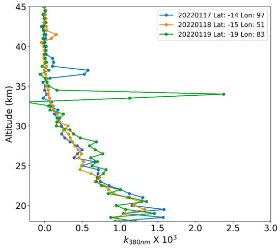
Figure 4.
Altitude profiles of aerosol extinction at 384 nm observed by the SAGE III satellite for three days during which elevated layers at altitudes greater than 30 km were seen.
The altitude variation in the range-corrected attenuated backscatter signals of the CALIPSO lidar observations during 17 and 19 January is shown in Figure 5, Figure 6 and Figure 7. These lidar measurement captured the volcanic plume between 20 km and 30 km of altitude very well. The plume seen in Figure 7 by the CALIPSO lidar also includes the region where the plume was observed by SAGE III (Figure 4) on 19 January 2022, showing that they both detected the enhancement in signal due to the same elevated stratospheric aerosol layer caused by the HTHH eruption. The CALIPSO and SAGE III observations are also consistent with the OMI observed columnar concentration shown in Figure 1. The HTHH plume observed by the SAGE III and CALIPSO lidar matched well with the spatial and temporal expansion of the plume as observed by the OMI satellite instrument. The remaining differences in Figure 1, Figure 4, Figure 5, Figure 6, Figure 7 and Figure 8 are due to different parts of the HTHH plume being observed at different times.
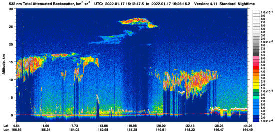
Figure 5.
Along-track curtain of attenuated backscatter signals observed by the CALIPSO lidar on 17 January 2022 showing the volcanic plume at altitudes from 20 km to 28 km, latitudes of ~8° S to 26° S, and longitudes of 149° E to 153° E. Image obtained from https://www-calipso.larc.nasa.gov/products/lidar/browse_images/std_v4_index.php (accessed on 12 July 2022).
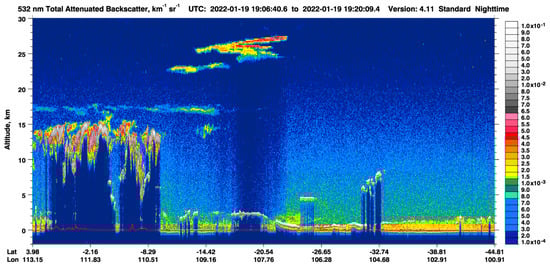
Figure 6.
Along-track curtain of attenuated backscatter signals observed by the CALIPSO lidar on 19 January 2022 showing the volcanic plume at altitudes from 22 km to 28 km, latitudes of ~10° S to 26° S, and longitudes of 106° E to 110° E. Image obtained from https://www-calipso.larc.nasa.gov/products/lidar/browse_images/std_v4_index.php (accessed on 12 July 2022).
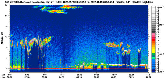
Figure 7.
Along-track curtain of attenuated backscatter signals observed by the CALIPSO lidar on 19 January 2022 showing the volcanic plume at altitudes from 28 km to >30 km, latitudes of ~2° S to 21° S, and longitudes of 83° E to 86° E. Image obtained from https://www-calipso.larc.nasa.gov/products/lidar/browse_images/std_v4_index.php (accessed on 12 July 2022).
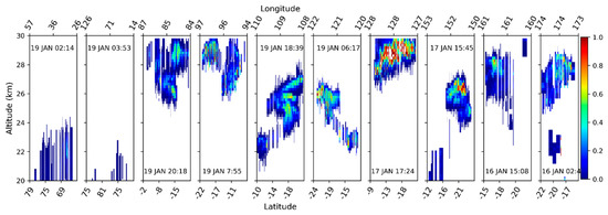
Figure 8.
Plot of aerosol extinction coefficients obtained from CALIPSO lidar observations on different days after the HTHH eruption. The altitude ranges from 20 km to 30 km.
Figure 8 shows the altitude variation in the aerosol extinction coefficients at 532 nm on selected days after the eruption (when the elevated layer was observed), as estimated using the CALIPSO lidar observations (level 2 data). We can see that the plume remained in an altitude band between 20 km and 30 km. It might even have existed above 30 km, as seen in the 19 January profile from SAGE III. However, the CALIPSO data are available only up to an altitude of 30 km. It is worth noting that the extinction coefficients often reached a very high value of 1, suggesting that the plume caused a significant reduction in the solar radiation reaching the surface.
3.1.3. Lagrangian Transport Modelling of the HTHH Plume Dispersal
The propagation of the SO2 plume injected by the HTHH volcanic eruption on 15 January 2022 has been simulated with the MPTRAC Lagrangian transport model. This model was already used in several studies for tracking the spread of volcanic eruption plumes [52,53,54]. The MPTRAC simulation was initiated at 04:15 UTC on 15 January 2022 at 175.38° W and 28° S. The altitude distribution and the spread of the plume immediately after the eruption have been detailed by many studies using observations from satellites, such as Himawari imagery [30]. The SO2 plume was initialized at this grid box at an altitude of 28 km. The SO2 mass was fixed at 400 kt. The meteorological inputs were provided by model level ERA5 hourly data files starting from the model initiation. The simulation was carried out from 15 January 2022 to 26 January 2022.
The simulated spread of the HTHH plume is shown in Figure 9 and Figure 10. Figure 9 shows the spatial distribution of the SO2 plume with colors representing the altitude of the plume in the stratosphere. Figure 10 is same as Figure 9, except that the colors show the column density of the SO2 plume in DU. Additional simulations were carried out by initiating the plume at different altitudes from 25 km to 35 km. However, the initial plume altitude of ~28 km provided the best match between the simulated transport with the OMI satellite data shown in Figure 1. The e-folding lifetime of SO2 in the stratosphere was kept fixed to 7 days. A comparison with the satellite observations shows that the plume injected into the stratosphere can be tracked for a long time using transport models such as MPTRAC.
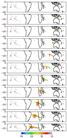
Figure 9.
Lagrangian transport simulation of the HTHH SO2 plume dispersal in the stratosphere from 16 to 26 January 2022. The initial plume height of the simulation was set to an altitude of 28 km. The initial latitude and longitude of the trajectories were set to the location of the HTHH eruption. The simulation starting time was 04:15 UTC on 15 January 2022. The colors show the altitude of the plume in km. The topmost panel is for 00:00 UTC on 16 January 2022. The location of the HTHH volcano is marked with a red x.
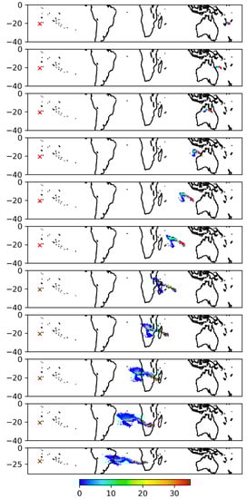
Figure 10.
Lagrangian transport simulation of the HTHH SO2 plume dispersal in the stratosphere from 16 to 26 January 2022, showing the column density of the stratospheric SO2 in DU. The topmost panel is for 00:00 UTC on 16 January 2022. The location of the HTHH volcano is marked with a red x.
3.2. Growth of the Sulfuric Acid Cloud and Its Optical Effects
A plot of monthly mean aerosol extinction coefficients with latitude at the wavelength of 384 nm from 2017 to 2021 using the SAGE III data is shown in Figure 11. It shows that a prominent aerosol layer above 20 km was not present throughout this period. There were years when the elevated layer was present below 20 km, which might have been caused by other volcanic eruptions. It is clear from Figure 11 that a state of unperturbed background stratospheric aerosol is rare due to injections of significant amounts of SO2 directly into the stratosphere by frequent volcanic eruptions. The sulfuric acid aerosol clouds are distributed globally over a period of months and have very high optical depths compared with background stratospheric aerosols. It typically takes a few years for the stratosphere to regain its natural background [11].
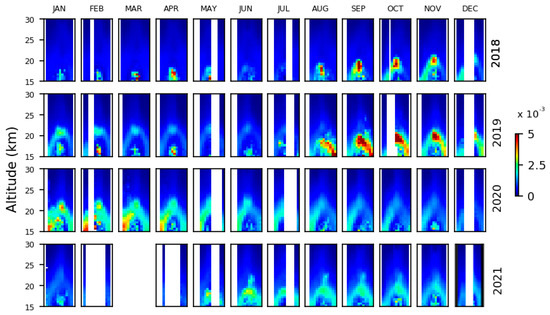
Figure 11.
Plots of monthly mean aerosol extinction coefficients at a 384 nm wavelength with latitude from 2017 to 2021 using SAGE III observations. The x-axis of each panel corresponds to a latitude range from 50° S to 50° N.
Figure 12 shows the altitude variation in the 384 nm aerosol extinction coefficients during the months following the 2022 HTHH volcanic eruption. Here we can see the overwhelming enhancement in aerosol extinction coefficients at the altitude range of 20 km to 26 km. This shows that the formation of the sulfuric acid clouds and subsequent growth in particle size caused a significant enhancement in the aerosol extinction coefficient. A histogram of aerosol extinction coefficients at 384 nm during the different months following the eruption is shown in Figure 13. This shows the dynamics of the sulfuric acid droplet growth happening at different altitudes each month. The post-eruption part of January 2022 appears to show an unperturbed state of the stratosphere, except for the occurrence of high aerosol extinction coefficient cases at the altitude of 33–40 km. With the progress of time, the occurrence of high aerosol extinction coefficient cases increased. The highest occurrences of aerosol extinction coefficient cases were observed during February 2022 and were located in the low latitude tropical belt. However, the frequency of occurrence were quite low compared with the March 2022–May 2022. The occurrences of high aerosol extinction coefficients were initially observed around an altitude of 25 km. However, after April 2022, the high aerosol extinction coefficient occurrence slowly shifted toward lower altitudes. During September 2022, high aerosol extinction coefficient occurrences were present at altitudes of 15 km to 26 km. This was due to the poleward transport of SO2 and sulfuric acid droplets and the subsequent growth in that area. At the same time, the concentration of sulfuric acid droplets reduced in the tropical region. As seen in Figure 12, the lower altitude occurrences were observed toward the poleward region and the higher altitude occurrences were observed over the tropical regions, mainly due to latitudinal variations in tropopause altitude.
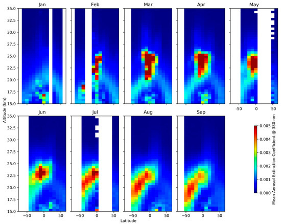
Figure 12.
Plots of monthly mean aerosol extinction coefficients at a 384 nm wavelength at different latitudes from January 2022 to September 2022 using SAGE III observations. The x-axis of each panel corresponds to a latitude range from 50° S to 50° N.
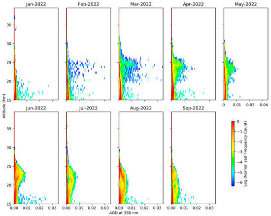
Figure 13.
Histogram of aerosol extinction coefficient observations at 384 nm by SAGE III/ISS during different months after the HTHH eruption.
The monthly mean Ångström exponent calculated using the 520 nm and 1021 nm aerosol extinction coefficient observations by SAGE III is plotted in Figure 14, and the colored histogram corresponding to this is plotted in Figure 15. The Ångström exponent (α) at each altitude has been computed by using the aerosol extinction coefficients measured by SAGE III at 520 nm and 1021 nm wavelengths,
where k(z)520nm and k(z)1021nm are the aerosol extinction coefficients at the 520 nm and 1021 nm wavelength channels of SAGE III, respectively, at altitude z.
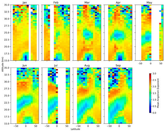
Figure 14.
Plots of monthly mean Ångström exponents with latitude using 520 nm and 1021 nm wavelength SAGE III observations during 2022. The x-axis of each panel corresponds to a latitude range from 50° S to 50° N.
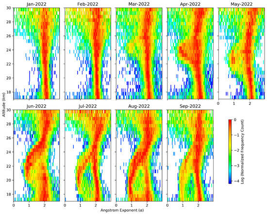
Figure 15.
Histogram of Ångström exponents calculated using the extinction coefficient observed at 520 nm and 1021 nm by SAGE III/ISS during the months after the HTHH eruption.
The Ångström exponent provides a measure of the sizes of the aerosol particles. A lower Ångström exponent corresponds to a larger size, and vice versa [55]. In the tropical region around the altitude of ~28 km during the February 2022, it can be seen that the Ångström exponents are reduced compared with those in the surrounding area. This region of reduced Ångström exponents grows from February to May due to the formation of sulfuric acid droplets, and subsequently due to coagulation, condensation, and coalescence. These droplets are transported toward the poles with time, altering the distribution of the aerosol particles therein. From June to September, the enhancement in the Ångström exponents is seen gradually at mid-latitudes due to poleward transport as well as the in-situ formation and growth of sulfuric acid droplets. Here it may be noted that the poleward transport in the southern hemisphere is much stronger compared with that in the northern hemisphere.
The method for calculating the surface area density (SAD) from the SAGE observations has been discussed in Thomason et al. [56]. Using the method described therein, the surface area densities for different months after the HTHH eruption were calculated using the aerosol extinction coefficient observations at 520 nm and 1021 nm wavelengths by SAGE III as given below.
Here, k1021 is the aerosol extinction coefficient of the 1021 nm channel in units of km−1 and r is the 520 nm to 1021 nm aerosol extinction coefficient ratio. This equation provides the surface area density in the units of µm2cm−3.
A plot of monthly mean surface area density with latitude during 2022 for different months is shown in Figure 16. The mean surface area density at a ~25 km altitude reached >15 µm2cm−3 from February 2022 to May 2022. This enhancement was mainly in the tropical region. Subsequently, the surface area density increase shifted towards the poleward latitudes but it was of a comparatively lower magnitude than that which occurred over the tropical region. The histogram plot (Supplementary Figure S1) of surface area density shows that the highest surface area density occurred during the month of February, reaching more than the 50 µm2cm−3. Over the following months, the occurrences of high surface area density reduced gradually. However, the frequency of occurrence of high surface area density of sulfuric acid droplets increased until May 2022. The frequency distribution of the surface area density and aerosol extinction coefficient are similar, as the aerosol extinction coefficient is directly dependent on the surface area density of the scatterers.
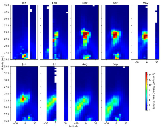
Figure 16.
Plots of monthly mean surface area density with latitude during 2022. The x-axis of each panel corresponds to a latitude range from 50° S to 50° N.
The altitude variation in the monthly mean of all SAGE III observations and the percentage enhancement in different months after the eruption with respect to January 2022 (pre-eruption) are shown in Figure 17. The peak enhancement occurred in the month of February 2022. However, the latitude–altitude extent of the sulfuric acid clouds was still limited in February. In the later months, the latitude as well as the altitude spread of the SO2 plume increased. However, peak enhancement was less than in February. The radiative impact would be much higher as it would be covering a larger latitude.
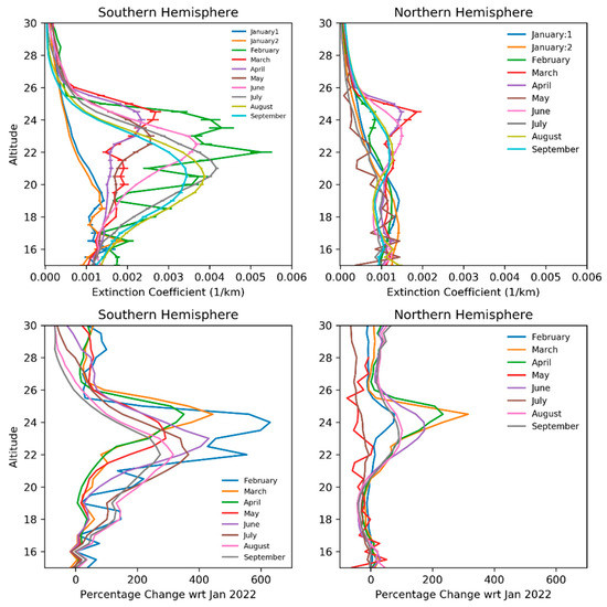
Figure 17.
Top panels: altitude variation in mean aerosol extinction coefficients of the SAGE-observed profiles for different months. January1 corresponds to days in January 2022 before the eruption, and January2 corresponds to days in January 2022 after the eruption. Bottom panels: altitude variation in percentage enhancement in aerosol extinction coefficient at 384 nm with respect to January 2022 (before eruption) in the northern and southern hemispheres.
Based on a simple radiative equilibrium model, Zhang et al. [39] computed that during the next 1–2 years the global mean surface air temperature will decrease by 0.0315–0.1118 °C due to an increase of 0.0019 in the global AOD. This impact is much less than that of the El Chichon eruption (AOD increase: 0.0325, SW flux reduction: 0.975 W m−2, global mean surface air temperature change: 0.3 °C). The recent update shows that the amount of SO2 injected into the stratosphere by HTHH is ~0.4 million tons, i.e., only 5.7% of that injected into the stratosphere by the El Chichon eruption (7 million tons).
The distribution of the sulfuric acid aerosols, which can be inferred from Figure 12, Figure 13, Figure 14, Figure 15, Figure 16, Figure 17 and Figure 18, has an asymmetrical distribution in the southern hemisphere. The aerosols were located at altitudes of 20–25 km during the initial months after the eruption, and they were located mainly in southern tropical belt. They were later dispersed to lower altitudes in the mid-latitude regions due to poleward transport. The spatial and temporal variations in the HTHH sulfuric acid aerosols are a direct manifestation of stratospheric transport processes such as the QBO, the Brewer Dobson circulation (BDC), and large scale Rossby waves. The BDC and large scale Rossby waves are responsible for the transport of sulfuric acid aerosols from the tropics to middle latitudes. Eventually, the aerosols will be removed by a variety of removal processes, such as mixing with tropospheric air due to transport across isentropic surfaces, cloud scavenging, etc. [11].
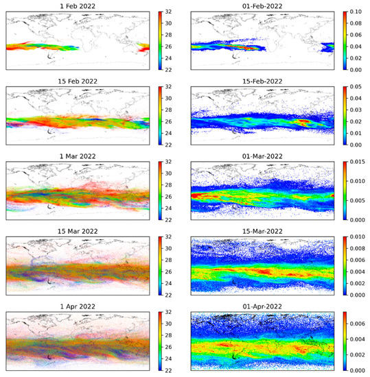
Figure 18.
Left panels: spatial distribution of air parcel altitudes (km) of the HTHH plume obtained from the Lagrangian transport simulation using the MPTRAC model. Right panels: spatial distribution of air parcel densities (/km2) of the HTHH plume.
It is interesting to note that during January–May, the aerosols were lying mostly in the tropical belt. However, in June, there was rapid poleward transport. This is directly related to the phase of the QBO. It has been reported in previous studies that during the easterly phase of the QBO, the stratospheric aerosols are compressed toward the tropics, and during the westerly phase of the QBO, the aerosols are transported toward the poles ([11] and references therein). During January 2022 to May 2022, the QBO was in its easterly phase at altitudes of 25–30 km, and during June, the QBO phase became westerly (https://acd-ext.gsfc.nasa.gov/Data_services/met/qbo/qbo.html, accessed on 5 November 2022).
3.3. Long-Term Lagrangian Transport Simulation of the HTHH Plume Dispersal
The Lagrangian transport simulation of the HTHH plume using the MPTRAC model described earlier was further continued until 1 April 2022. The results of the MPTRAC simulation for selected days are shown in Figure 18. The MPTRAC simulation is reproducing the spread of the sulfuric acid clouds as observed by SAGE III. The dominant confinement of the plume in the southern hemisphere is also seen in the simulations.
4. Summary
In this study, we investigated the global spread of the HTHH volcanic eruption using OMI, SAGE III, and CALIPSO lidar data and Lagrangian transport simulations obtained using the MPTRAC model. During the initial phase of the spread, the dominant westward propagation of the SO2 plume encircled the globe in the 0–30° S latitude band within 21 ± 2 days. The average speed of the westward spread inferred by the plume spread length per day was found to be about 2500 ± 500 km/day. The difference in the transport velocity during the different days is mainly attributed to the difference in the wind speeds at the different altitudes at which the plume was propagating. In addition, the plume coverage slowly expanded to northern and southern hemisphere latitudes due to the dispersal process. The sulfuric acid cloud started appearing in the stratosphere within just a few days due to the formation of tiny sulfuric acid droplets because of the reaction between SO2 and OH radicals and subsequent growth due to coagulation. This was observed in the SAGE III data as well as in the CALIPSO data, and the frequent occurrence of high aerosol extinction coefficient values in the SAGE III and CALIPSO altitude profiles was observed. These high aerosol extinction coefficient elevated layers were mostly centered between 20–26 km altitudes. The peak enhancement of extinction was as large as 600% during February at an altitude of about 24 km. The peak AOD enhancement due to the sulfuric acid cloud formation after the HTHH eruption was about half of that caused by the Mt. Pinatubo eruption. The global spread of the Tonga plume in the stratosphere has been simulated using the MPTRAC Lagrangian transport model. The simulated plume distribution is matching well with the observations of the OMI satellite. The progression of the sulfuric acid cloud formation and its transport with latitude and altitude has been visualized using the altitude profiles and histograms of the aerosol extinction coefficient, Ångström exponent, and surface area density.
The spread of the HTHH SO2 and sulfuric acid clouds is asymmetric, being largely confined to the southern hemisphere. This asymmetrical distribution will cause an asymmetrical radiative effect. It will be interesting to see how this asymmetrical distribution impacts the atmospheric circulation processes.
The perturbation caused by the HTHH eruption will affect almost all components of the earth–atmosphere system through feedback effects due to perturbation of the radiative fluxes over all parts of the atmosphere. The eruption will also affect the composition of the stratosphere. However, the potential radiative impact of the HTHH eruption is likely to be much less than that of the Mt. Pinatubo eruption as the total amount of material injected in the stratosphere is much lower. Accurate estimates of the overall radiative and climatic effects can only be ascertained about 1–2 years after the eruption. It will be important to see how the eruption affects the global temperature and major circulation patterns (such as the Indian summer monsoon, El-Nino, etc.), which were reported to have been affected by earlier volcanic eruptions.
Supplementary Materials
The following supporting information can be downloaded at: https://www.mdpi.com/article/10.3390/atmos13122055/s1, Figure S1: Histogram of surface area density computed using SAGE III/ISS data during different months after the HTHH eruption.
Author Contributions
Conceptualization, M.K.M.; methodology, M.K.M. and L.H.; software, M.K.M. and L.H.; validation, M.K.M. and L.H.; formal analysis, M.K.M.; investigation, M.K.M. and L.H.; resources, M.K.M., L.H. and P.K.T.; data curation, M.K.M.; writing—original draft preparation, M.K.M.; writing—review and editing, M.K.M. and L.H.; visualization, M.K.M.; supervision, P.K.T. All authors have read and agreed to the published version of the manuscript.
Funding
This research received no external funding.
Institutional Review Board Statement
Not applicable.
Data Availability Statement
The MPTRAC model (Hoffmann et al., 2016, https://doi.org/10.1002/2015JD023749, accessed on 5 November 2022; Hoffmann et al., 2022, https://doi.org/10.5194/gmd-15-2731-2022, accessed on 5 November 2022) is available under the terms and conditions of the GNU General Public License, Version 3, via the repository at https://github.com/slcs-jsc/mptrac (last access: 10 January 2022) and has been archived on Zenodo (https://doi.org/10.5281/zenodo.5714528, accessed on 5 November 2022; Hoffmann et al., 2021). SAGE III/ISS data: NASA/LARC/SD/ASDC (2017). SAGE III/ISS L2 Solar Event Species Profiles (HDF5) V052 (data set). NASA Langley Atmospheric Science Data Center DAAC. Retrieved from https://doi.org/10.5067/ISS/SAGEIII/SOLAR_HDF5_L2-V5.2, accessed on 5 November 2022. CALIPSO data: NASA/LARC/SD/ASDC (2018). CALIPSO Lidar Level 2 Aerosol Profile, V4-21 (data set). NASA Langley Atmospheric Science Data Center DAAC. Retrieved from https://doi.org/10.5067/CALIOP/CALIPSO/CAL_LID_L2_05kmAPro-Standard-V4-21, accessed on 5 November 2022. NASA/LARC/SD/ASDC (2016). CALIPSO Lidar Level 2 Aerosol Profile, Provisional V3-41 (data set). NASA Langley Atmospheric Science Data Center DAAC. Retrieved from https://doi.org/10.5067/CALIOP/CALIPSO/CAL_LID_L2_05kmAPro-Prov-V3-41, accessed on 5 November 2022.
Acknowledgments
We acknowledge ASDC, NASA, and the Earthdata Center, NASA for providing access to SAGE III, CALIPSO, and OMI data. We acknowledge the Juelich Supercomputing Centre for providing access to computer and storage resources on its HPC systems.
Conflicts of Interest
The authors declare no conflict of interest.
References
- Kremser, S.; Thomason, L.; von Hobe, M.; Hermann, M.; Deshler, T.; Timmreck, C.; Toohey, M.; Stenke, A.; Schwarz, J.P.; Weigel, R.; et al. Stratospheric aerosol-Observations, processes, and impact on climate. Rev. Geophys. 2016, 54, 278–335. [Google Scholar] [CrossRef]
- Marshall, L.R.; Maters, E.C.; Schmidt, A.; Timmreck, C.; Robock, A.; Toohey, M. Volcanic effects on climate: Recent advances and future avenues. Bull. Volcanol. 2022, 84, 54. [Google Scholar] [CrossRef]
- Robock, A. Volcanic eruptions and climate. Rev. Geophys. 2000, 38, 191–219. [Google Scholar] [CrossRef]
- Di Martino, R.; Capasso, G.; Camarda, M.; De Gregorio, S.; Prano, V. Deep CO2 release revealed by stable isotope and dif-fuse degassing surveys at Vulcano (Aeolian Islands) in 2015–2018. J. Volcanol. Geotherm. Res. 2020, 401, 106972. [Google Scholar] [CrossRef]
- Di Martino, R.M.R.; Camarda, M.; Gurrieri, S.; Valenza, M. Asynchronous changes of CO2, H2, and He concentrations in soil gases: A theoretical model and experimental results. J. Geophys. Res. Solid Earth 2016, 121, 1565–1583. [Google Scholar] [CrossRef]
- Gurrieri, S.; Liuzzo, M.; Giuffrida, G.; Boudoire, G. The first observations of CO2 and CO2/SO2 degassing variations rec-orded at Mt. Etna during the 2018 eruptions followed by three strong earthquakes. Ital. J. Geosci. 2021, 140, 95–106. [Google Scholar] [CrossRef]
- Sioris, C.E.; Malo, A.; McLinden, C.A.; D’Amours, R. Direct injection of water vapor into the stratosphere by volcanic erup-tions. Geophys. Res. Lett. 2016, 43, 7694–7700. [Google Scholar] [CrossRef]
- Nagai, T.; Liley, B.; Sakai, T.; Shibata, T.; Uchino, O. Post-Pinatubo evolution and subsequent trend of the stratospheric aer-osol layer observed by mid-latitude lidars in both hemispheres. SOLA 2010, 6, 69–72. [Google Scholar] [CrossRef][Green Version]
- Prata, A.J.; Carn, S.A.; Stohl, A.; Kerkmann, J. Long range transport and fate of a stratospheric volcanic cloud from Soufrière Hills volcano, Montserrat. Atmos. Chem. Phys. 2007, 7, 5093–5103. [Google Scholar] [CrossRef]
- Rizi, V.; Masci, F.; Redaelli, G.; Di Carlo, P.; Iarlori, M.; Visconti, G.; Thomason, L.W. Lidar and SAGE II observations of Shishaldin Volcano aerosols and lower stratospheric transport. Geophys. Res. Lett. 2000, 27, 3445–3448. [Google Scholar] [CrossRef]
- Hamill, P.; Jensen, E.J.; Russell, P.B.; Bauman, J.J. The life cycle of stratospheric aerosol particles. Bull. Am. Meteorol. Soc. 1997, 78, 1395–1410. [Google Scholar] [CrossRef]
- Chen, K.; Ning, L.; Liu, Z.; Liu, J.; Yan, M.; Sun, W.; Li, L.; Shi, Z. Modulating and Resetting Impacts of Different Volcanic Eruptions on North Atlantic SST Variations. J. Geophys. Res. Atmos. 2022, 127, e2021JD036246. [Google Scholar] [CrossRef]
- Crutzen, P.J. Albedo Enhancement by Stratospheric Sulfur Injections: A Contribution to Resolve a Policy Dilemma? Clim. Chang. 2006, 77, 211–220. [Google Scholar] [CrossRef]
- Guzewich, S.D.; Oman, L.D.; Richardson, J.A.; Whelley, P.L.; Bastelberger, S.T.; Young, K.E.; Bleacher, J.E.; Fauchez, T.J.; Kopparapu, R.K. Volcanic Climate Warming Through Radiative and Dynamical Feedbacks of SO2 Emissions. Geophys. Res. Lett. 2022, 49, e2021GL096612. [Google Scholar] [CrossRef]
- Dutton, E.G.; Christy, J.R. Solar radiative forcing at selected locations and evidence for global lower tropospheric cooling following the eruptions of El Chichón and Pinatubo. Geophys. Res. Lett. 1992, 19, 2313–2316. [Google Scholar] [CrossRef]
- Minnis, P.; Harrison, E.F.; Stowe, L.L.; Gibson, G.G.; Denn, F.M.; Doelling, D.R.; Smith, W.L. Radiative climate forcing by the Mount Pinatubo eruption. Science 1993, 259, 1411–1415. [Google Scholar] [CrossRef] [PubMed]
- Coffey, M.T. Observations of the impact of volcanic activity on stratospheric chemistry. J. Geophys. Res. Atmos. 1996, 101, 6767–6780. [Google Scholar] [CrossRef]
- Solomon, S. Stratospheric ozone depletion: A review of concepts and history. Rev. Geophys. 1999, 37, 275–316. [Google Scholar] [CrossRef]
- Tabazadeh, A.; Turco, R.P. Stratospheric chlorine injection by volcanic eruptions: HCl scavenging and implication for ozone. Science 1993, 260, 1082–1086. [Google Scholar] [CrossRef]
- McCormick, M.P.; Thomason, L.W.; Trepte, C.R. Atmospheric effects of the Mt Pinatubo eruption. Nature 1995, 373, 399–404. [Google Scholar] [CrossRef]
- Stenchikov, G.L.; Kirchner, I.; Robock, A.; Graf, H.-F.; Antuña-Marrero, J.C.; Grainger, R.G.; Lambert, A.; Thomason, L. Ra-diative forcing from the 1991 Mount Pinatubo volcanic eruption. J. Geophys. Res. Atmos. 1998, 103, 13837–13857. [Google Scholar] [CrossRef]
- Harries, J.E.; Futyan, J.M. On the stability of the Earth’s radiative energy balance: Response to the Mt. Pinatubo eruption. Geophys. Res. Lett. 2006, 33, L23814. [Google Scholar] [CrossRef]
- Angell, J.K. Stratospheric warming due to Agung, El Chichón, and Pinatubo taking into account the quasi-biennial oscilla-tion. J. Geophys. Res. Atmos. 1997, 102, 9479–9485. [Google Scholar] [CrossRef]
- Antuña-Marrero, J.C.; Robock, A.; David, C.; Thomason, L.; Stenchikov, G.L.; Zhou, J.; Barnes, J. Spatial and temporal varia-bility of the stratospheric aerosol cloud produced by the 1991 Mount Pinatubo eruption. J. Geophys. Res. Atmos. 2003, 108, 4624. [Google Scholar] [CrossRef]
- Aquila, V.; Oman, L.; Stolarski, R.S.; Colarco, P.R.; Newman, P. Dispersion of the volcanic sulfate cloud from a Mount Pinatubo-like eruption. J. Geophys. Res. Atmos. 2012, 117, D06216. [Google Scholar] [CrossRef]
- Bingen, C.; Fussen, D.; Vanhellemont, F. A global climatology of stratospheric aerosol size distribution parameters derived from SAGE II data over the period 1984–2000: 1. Methodology and climatological observations. J. Geophys. Res. Atmos. 2004, 109, D06201. [Google Scholar] [CrossRef]
- Deshler, T.; Hervig, M.E.; Hofmann, D.J.; Rosen, J.M.; Liley, J.B. Thirty years of in situ stratospheric aerosol size distribution measurements from Laramie, Wyoming (41°N), using balloon-borne instruments. J. Geophys. Res. Atmos. 2003, 108, 4167. [Google Scholar] [CrossRef]
- Vömel, H.; Evan, S.; Tully, M. Water vapor injection into the stratosphere by Hunga Tonga-Hunga Ha’apai. Science 2022, 377, 1444–1447. [Google Scholar] [CrossRef]
- Carr, J.L.; Horváth, A.; Wu, D.L.; Friberg, M.D. Stereo Plume Height and Motion Retrievals for the Record-Setting Hunga Tonga-Hunga Ha’apai Eruption of 15 January 2022. Geophys. Res. Lett. 2022, 49, e2022GL098131. [Google Scholar] [CrossRef]
- Gupta, A.K.; Bennartz, R.; Fauria, K.E.; Mittal, T. Timelines of plume characteristics of the Hunga Tonga-Hunga Ha’apai eruption sequence from 19 December 2021 to 16 January 2022: Himawari-8 observations. Earth Space Sci. Open Arch. 2022. [CrossRef]
- Proud, S.R.; Prata, A.T.; Schmauβ, S. The January 2022 eruption of Hunga Tonga-Hunga Ha’apai volcano reached the meso-sphere. Science 2022, 378, 554–557. [Google Scholar] [CrossRef] [PubMed]
- Aa, E.; Zhang, S.; Wang, W.; Erickson, P.J.; Qian, L.; Eastes, R.; Harding, B.J.; Immel, T.J.; Karan, D.K.; Daniell, R.E.; et al. Pronounced suppression and X-pattern merging of equatorial ionization anomalies after the 2022 Tonga volcano eruption. J. Geophys. Res. Space Phys. 2022, 127, e2022JA030527. [Google Scholar] [CrossRef] [PubMed]
- Adam, D. Tonga volcano eruption created puzzling ripples in Earth’s atmosphere. Nature 2022, 601, 497. [Google Scholar] [CrossRef]
- Harding, B.J.; Wu, Y.J.; Alken, P.; Yamazaki, Y.; Triplett, C.C.; Immel, T.J.; Gasque, L.C.; Mende, S.B.; Xiong, C. Impacts of the January 2022 Tonga volcanic eruption on the ionospheric dynamo: ICON-MIGHTI and Swarm observa-tions of extreme neutral winds and currents. Geophys. Res. Lett. 2022, 49, e2022GL098577. [Google Scholar] [CrossRef]
- Harrison, G. Pressure anomalies from the January 2022 Hunga Tonga-Hunga Ha’apai eruption. Weather 2022, 77, 87–90. [Google Scholar] [CrossRef]
- Wright, C.J.; Hindley, N.P.; Alexander, M.J.; Barlow, M.; Hoffmann, L.; Mitchell, C.N.; Prata, F.; Bouillon, M.; Carstens, J.; Clerbaux, C.; et al. Surface-to-space atmospheric waves from Hunga Tonga–Hunga Ha’apai eruption. Nature 2022, 609, 741–746. [Google Scholar] [CrossRef]
- Yamada, M.; Ho, T.; Mori, J.; Nishikawa, Y.; Yamamoto, M. Tsunami triggered by the Lamb wave from the 2022 Tonga vol-canic eruption and transition in the offshore Japan region. Geophys. Res. Lett. 2022, 49, e2022GL098752. [Google Scholar] [CrossRef]
- Sellitto, P.; Podglajen, A.; Belhadji, R.; Boichu, M.; Carboni, E.; Cuesta, J.; Duchamp, C.; Kloss, C.; Siddans, R.; Bègue, N.; et al. The unexpected radiative impact of the Hunga Tonga eruption of 15th January 2022. Commun. Earth Environ. 2022, 3, 288. [Google Scholar] [CrossRef]
- Zhang, H.; Wang, F.; Li, J.; Duan, Y.; Zhu, C.; He, J. Potential Impact of Tonga Volcano Eruption on Global Mean Surface Air Temperature. J. Meteorol. Res. 2022, 36, 1–5. [Google Scholar] [CrossRef]
- Millán, L.; Santee, M.L.; Lambert, A.; Livesey, N.J.; Werner, F.; Schwartz, M.J.; Pumphrey, H.C.; Manney, G.L.; Wang, Y.; Su, H.; et al. The Hunga Tonga-Hunga Ha’apai Hydration of the Stratosphere. Geophys. Res. Lett. 2022, 49, e2022GL099381. [Google Scholar] [CrossRef]
- Li, C.; Krotkov, N.A.; Leonard, P.; Joiner, J. OMI/Aura Sulphur Dioxide (SO2) Total Column 1-orbit L2 Swath 13 × 24 km V003; Goddard Earth Sciences Data and Information Services Center (GES DISC): Greenbelt, MD, USA, 2020. [Google Scholar] [CrossRef]
- Carn, S.A.; Krueger, A.J.; Krotkov, N.A.; Yang, K.; Evans, K. Tracking volcanic sulfur dioxide clouds for aviation hazard mitigation. Nat. Hazards 2009, 51, 325–343. [Google Scholar] [CrossRef]
- Yang, K.; Krotkov, N.A.; Krueger, A.J.; Carn, S.A.; Bhartia, P.K.; Levelt, P.F. Retrieval of Large Volcanic SO2 columns from the Aura Ozone Monitoring Instrument (OMI): Comparisons and Limitations. J. Geophys. Res. 2007, 112, D24S43. [Google Scholar] [CrossRef]
- Cisewski, M.; Zawodny, J.; Gasbarre, J.; Eckman, R.; Topiwala, N.; Rodriguez-Alvarez, O.; Cheek, D.; Hall, S. The Strato-spheric Aerosol and Gas Experiment (SAGE III) on the International Space Station (ISS) Mission. In Sensors, Systems, and Next-Generation Satellites XVIII; SPIE: Bellingham, WA, USA, 2014; Volume 9241, pp. 59–65. [Google Scholar] [CrossRef]
- Hoffmann, L.; Baumeister, P.F.; Cai, Z.; Clemens, J.; Griessbach, S.; Günther, G.; Heng, Y.; Liu, M.; Mood, K.H.; Stein, O.; et al. Massive-Parallel Trajectory Calculations version 2.2 (MPTRAC-2.2): Lagrangian transport simulations on graphics pro-cessing units (GPUs). Geosci. Model Dev. 2022, 15, 2731–2762. [Google Scholar] [CrossRef]
- Hoffmann, L.; Rößler, T.; Griessbach, S.; Heng, Y.; Stein, O. Lagrangian transport simulations of volcanic sulfur dioxide emissions: Impact of meteorological data products. J. Geophys. Res. Atmos. 2016, 121, 4651–4673. [Google Scholar] [CrossRef]
- Hersbach, H.; Bell, B.; Berrisford, P.; Hirahara, S.; Horanyi, A.; Muñoz-Sabater, J.; Nicolas, J.; Peubey, C.; Radu, R.; Schepers, D.; et al. The ERA5 global reanalysis. Q. J. R. Meteorol. Soc. 2020, 146, 1999–2049. [Google Scholar] [CrossRef]
- Robock, A.; Matson, M. Circumglobal transport of the El Chichón volcanic dust cloud. Science 1983, 221, 195–197. [Google Scholar] [CrossRef] [PubMed]
- Bluth, G.J.S.; Doiron, S.D.; Schnetzler, C.C.; Krueger, A.J.; Walter, L.S. Global tracking of the SO2 clouds from the June, 1991 Mount Pinatubo eruptions. Geophys. Res. Lett. 1992, 19, 151–154. [Google Scholar] [CrossRef]
- Russell, P.B.; Livingston, J.M.; Pueschel, R.F.; Bauman, J.J.; Pollack, J.B.; Brooks, S.L.; Hamill, P.; Thomason, L.W.; Stowe, L.L.; Deshler, T.; et al. Global to microscale evolution of the Pinatubo volcanic aerosol derived from diverse measurements and analyses. J. Geophys. Res. Atmos. 1996, 101, 18745–18763. [Google Scholar] [CrossRef]
- Trepte, C.R.; Veiga, R.E.; McCormick, M.P. The poleward dispersal of Mount Pinatubo volcanic aerosol. J. Geophys. Res. At-mos. 1993, 98, 18563–18573. [Google Scholar] [CrossRef]
- Wu, X.; Griessbach, S.; Hoffmann, L. Equatorward dispersion of a high-latitude volcanic plume and its relation to the Asian summer monsoon: A case study of the Sarychev eruption in 2009. Atmos. Chem. Phys. 2017, 17, 13439–13455. [Google Scholar] [CrossRef]
- Wu, X.; Griessbach, S.; Hoffmann, L. Long-range transport of volcanic aerosol from the 2010 Merapi tropical eruption to Antarctica. Atmos. Chem. Phys. 2018, 18, 15859–15877. [Google Scholar] [CrossRef]
- Cai, Z.; Griessbach, S.; Hoffmann, L. Improved estimation of volcanic SO2 injections from satellite retrievals and Lagrangi-an transport simulations: The 2019 Raikoke eruption. Atmos. Chem. Phys. 2022, 22, 6787–6809. [Google Scholar] [CrossRef]
- Malinina, E.; Rozanov, A.; Rieger, L.; Bourassa, A.; Bovensmann, H.; Burrows, J.P.; Degenstein, D. Stratospheric aerosol characteristics from space-borne observations: Extinction coefficient and Ångström exponent. Atmos. Meas. Tech. 2019, 12, 3485–3502. [Google Scholar] [CrossRef]
- Thomason, L.W.; Burton, S.P.; Luo, B.-P.; Peter, T. SAGE II measurements of stratospheric aerosol properties at non-volcanic levels. Atmos. Chem. Phys. 2008, 8, 983–995. [Google Scholar] [CrossRef]
Publisher’s Note: MDPI stays neutral with regard to jurisdictional claims in published maps and institutional affiliations. |
© 2022 by the authors. Licensee MDPI, Basel, Switzerland. This article is an open access article distributed under the terms and conditions of the Creative Commons Attribution (CC BY) license (https://creativecommons.org/licenses/by/4.0/).