Article

Traffic Density and Air Pollution: Spatial and Seasonal Variations of Nitrogen Dioxide and Ozone in Jamaica, New York

1
Department of Earth and Physical Sciences, City University of New York-York College, 94-20 Guy R. Brewer Blvd., Jamaica, NY 11451, USA
2
Department of Earth, Environmental and Geospatial Sciences, CUNY-Lehman College, 250 Bedford Park Blvd. W, Bronx, NY 10468, USA
3
Department of Chemistry and Environmental Science, CUNY- Medgar Evers College, 1638 Bedford Ave., Brooklyn, NY 11225, USA
4
Department of Physical Therapy, School of Sciences, Hampton University, 100 E Queen St., Hampton, VA 23669, USA
*
Author to whom correspondence should be addressed.
Atmosphere 2022, 13(12), 2042; https://doi.org/10.3390/atmos13122042
Submission received: 22 November 2022 / Revised: 2 December 2022 / Accepted: 2 December 2022 / Published: 6 December 2022
(This article belongs to the Special Issue Feature Papers in Air Quality)

Abstract

:
Nitrogen dioxide (NO2) and ground-level ozone (O3) pose significant public health concerns in urban areas. This study assessed the safety level of NO2 and described spatial and seasonal variations of NO2 and O3 in Jamaica Center, New York, using low-cost diffusion tubes at six high-traffic (HT) and three low-traffic (LT) sites over two-week intervals in summer, winter, and fall of 2019. When annualized, the highest NO2 level (33.90 μg/m3) was below the safety threshold (99.6 μg/m3). Mean concentrations of NO2 samples were significantly higher at HT sites (35.79 μg/m3; 95%CI: 32.81–38.77) compared to LT sites (25.29 μg/m3; 95%CI: 11.73–28.85), p = 0.002, and during fall (38.14 μg/m3; 95%CI: 31.18–45.11) compared to winter (25.53 μg/m3; 95%CI: 20.84–30.22). There was no significant difference in O3 levels between the fall (51.68 μg/m3; 95%CI: 44.70–58.67) and summer (46.43 μg/m3; 95%CI: 35.25–57.61), p = 0.37, and between HT sites (48.51 μg/m3; 95%CI: 40.39–56.63) and LT sites (50.14 μg/m3; 95%CI: 43.98–56.30), p = 0.79. Our results demonstrate the feasibility of low-cost air monitoring and the need for emission control policies along major corridors mainly in fall and summer, especially with the rapid commercial and economic development underway in Jamaica Center.

1. Introduction

Anthropogenic sources of nitrogen dioxide (NO2) and ground-level ozone (O3) are ubiquitous in urban areas [1] and are a significant public health concern due to their harmful impacts, especially respiratory symptoms, and cardiovascular disease [2]. In general, NO2 has been considered a useful indicator for air pollution measurement from motor vehicle sources and can react with other chemicals in the air to form O3 [3,4]. NO2 and NO (nitric oxide) are the two principal types of nitrogen oxides (NOx) that are associated with combustion sources, and exhaust from vehicular traffic is the main outdoor source of NO2 [5]. The reaction path of NOx generally favors NO2 production and is temperature-dependent, and concentrations vary among the seasons. NOx formation has shown greater dependence on direct source emission rather than on photochemical processes; hence, NO2 levels are typically higher in the winter than in summer [6,7,8]. In summer, minimal NO2 levels are observed as a precursor to O3 in sunlight or high-energy radiation [9]. This photochemical reaction splits NO2 into NO and a single oxygen (O) atom, shown in the reaction below (R1). The single O atom combines with a diatomic (O2) oxygen molecule to produce O3 (R2); then, O3 reacts with NO to form NO2 and O2 (R3).
A net gain in O3 also occurs when high amounts of NOx and volatile organic compounds (VOCs) come from both natural and industrial sources, leading to a greater rate of O3 formation. Therefore, photochemical reactions involving VOCs and NOx are the main O3 sources formed when O2 and the single O atom, in the presence of a third-body molecule, absorb the heat of the reaction. The short-lived O atom is highly reactive and can be generated via the photolysis of NO2 or by the ionization of O2. When NO2 is photolyzed, the resulting O atom rapidly becomes O3 in a photostationary state. Either in the absence or at very low concentrations of VOCs, O3 reaches a steady-state concentration depending on solar intensity, ambient temperature, and the ratio of NO2 concentration to NO concentration. Under this condition, one NO2 molecule is converted via photolysis into an O3 molecule and a NO molecule; then, O3 is consumed by NO to regenerate a NO2 molecule. This cycle results in zero accumulation of O3 concentration. In other words, when reactions 1, 2, and 3 occur at the same rate, there is no net gain in O3 [10]. High temperatures from vehicular combustion and sunlight cause such chemical reactions between NOX and VOCs. Nitrate particles that result from NOx can make the air hazy, resulting in poor visibility [11]. NO2 can also interact with water, oxygen, and other chemicals to create acid rain.
NO2 + sunlight → NO + O (R1)
O + O2 → O3 (R2)
NO + O3 → NO2 + O2 (R3)
Since NO is rapidly oxidized in ambient air to form NO2 by available oxidants such as O3 and VOCs, NO2 is thus considered a primary air pollutant due to its swift oxidation velocity [12]. Additionally, NO2 is the most toxic form of NOx; as such, its spatial and seasonal measurements are important for a better understanding of the ambient conditions that favor its persistence, including the formation of O3 and harmful exposure levels. While ambient concentrations of NO and NO2 vary widely, together, they can exceed a total concentration of 500 μg/m3 in dense urban areas such as Jamaica Center. Further, according to Jarvis et al. [12], 90–95% of the NOx released in ambient air is usually emitted as NO and only 5–10% as NO2. Inhalation of air with high concentrations of NO2 is associated with severe chronic respiratory problems.
As a secondary pollutant, ambient O3 concentrations vary, as they are influenced by site-specific conditions such as prevailing wind patterns, the architecture of the built environment, the severity of air pollution, and daytime temperatures [13,14]. Maximum exposure to ambient O3 tends to be strongly correlated with daytime temperatures [15], particularly in the summertime. In the presence of sunlight and NOx, temperature directly influences O3 production by increasing the rates of chemical reactions and emission of VOCs, resulting in unhealthy O3 levels on hot sunny days in urban environments. On the other hand, it is possible for O3 to reach high levels during the cool fall and cold winter months [16]. Continued exposure to NO2 or O3 can lead to various health effects; it can exacerbate asthma; decrease lung function and quality of life; cause irritation, inflammation, and permanent lung tissue damage; and predispose cardiovascular disease and immune system impairment [16]. The World Health Organization (WHO) suggests a one-hour NO2 threshold of 105 ppb (200 μg/m3) and an annual average threshold of 21 ppb (40 μg/m3) based on respiratory illness in children [17]. Near-source NO2 and O3 levels are characterized by high spatial and temporal variability depending on their location relative to the source, meteorology, varying emission rates, and other factors [18].
Since current ambient air-quality monitoring in urban areas relies on fixed monitoring sites, there is possibility of underestimating actual NO2 and O3 exposures within the community. Hence, low-cost strategies and technologies have become more valuable. Passive air diffusion tubes are efficient cost-friendly ways to spatially measure air pollution concentrations in a variety of environments, as they are small in size [19,20]. Additionally, given their low cost, they offer a viable option to supplement data from networks of fixed-site air pollution monitors since they can be deployed widely in communities or enable simultaneous individual-level air pollution measurements. This approach can generate data that can be useful in monitoring exposure to outdoor air pollution, particularly in community and population studies [21]. Existing monitoring networks have limited spatial coverage, typically with few stations in urban locations. In addition, most existing monitoring networks have insufficient density to capture small-scale (within-city) variations of air pollution, which can be quite substantial for certain pollutants [22,23,24].
As an initial step to evaluate the levels of air pollution and its potential impact on the health of residents of Jamaica Center, New York, we investigated the spatial and seasonal variations of NO2 and O3 in a heavily trafficked area using passive diffusion tubes as a low-cost air quality monitoring method. The aim of this study is to (1) assess safety levels of NO2 at the study sites; (2) identify the spatial trends in NO2 and O3 concentrations between heavy and low-traffic areas of Jamaica, NY; and (3) describe the seasonal variations in NO2 and O3 concentrations between heavy- and low-traffic areas of Jamaica, NY. The findings of this study will contribute to current air pollution data that examine the effectiveness of low-cost technologies for further long-term assessment of air pollution. They may also inform strategies to improve air quality and mitigate the potential adverse environmental and public health effects of major air pollutants.

2. Materials and Methods

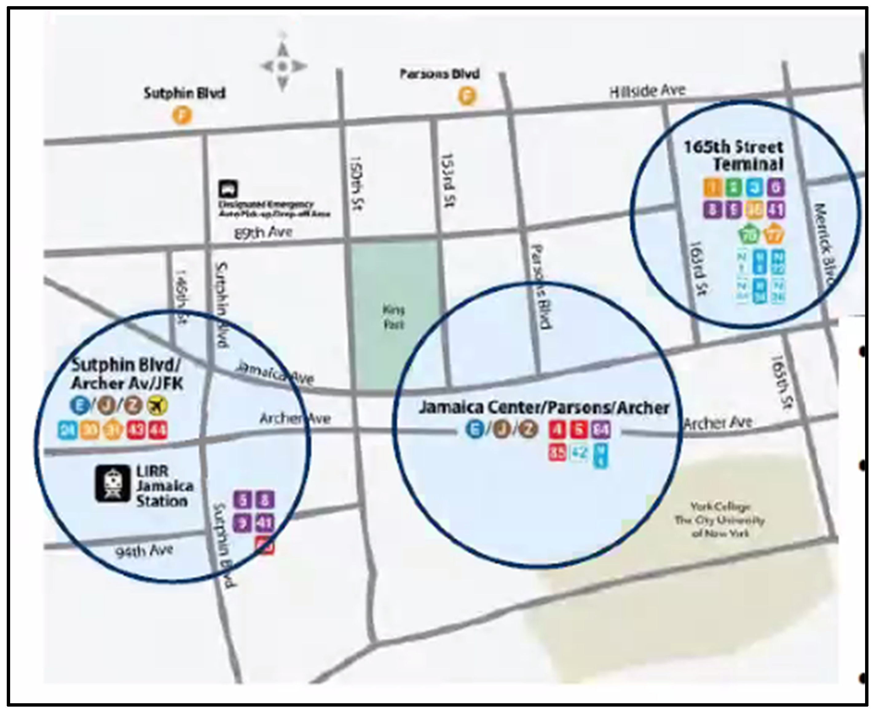
2.1. Location and Site Description

This study was conducted in 2019 in Jamaica Center (40.7021° N, 73.8009° W), a transportation hub of an industrialized urban area and a major commuter rail and bus station of the New York City (NYC) Metropolitan Transportation Authority (MTA). Jamaica Center is connected to two other transportation hubs that are less than one mile away: the Sutphin Boulevard transportation hub at 0.4 miles to the west and the 163rd Street Bus Terminal at 0.7 miles to the northeast (Figure 1). These connections contribute to high transfers between buses and trains, with notably more than fifty bus lines in Jamaica Center. More than forty thousand commuters enter the downtown Jamaica area daily. Thus, high pedestrian volumes are concentrated along the major corridors of Jamaica and Archer Avenues, which house several small businesses. The numerous commercial and transportation activities along these corridors with high traffic of passenger cars, diesel trucks, and MTA buses constitute a major source of pollution in this area (Figure S1).
Neighborhoods contiguous to Jamaica Center are heavily impacted by air pollution emitted from vehicular traffic. In 2018, respiratory-related health issues were disproportionately higher in Jamaica than in NYC, and the average life expectancy was 0.7 years shorter than NYC overall. According to the NYC Community Health Profile, the asthma hospitalization rate for children ages 5–14 in Jamaica alone was 32 out of every 10,000 children [25]. The rate of avoidable hospitalizations (per 100,000) among adults in Jamaica (1602) was higher than the citywide rate (1033) and much higher than affluent towns (426); diabetes (16%) and hypertension (37%) rates for Jamaica residents were both higher than the rest of NYC (11% and 28%), respectively. Nine monitoring stations were selected based on traffic densities of six heavily trafficked (HT) roadways along Jamaica and Archer Avenues and along three adjacent streets with low traffic flow (LT). Additional location details of the sites are shown in Table 1. According to the Environmental Protection Agency (EPA), high concentrations of pollutants are expected along heavily trafficked roadways compared to low-traffic areas [26]. Concentrations of NO2 were measured during the winter, summer, and fall seasons, whereas samples of O3 were collected during the summer and fall only.

2.2. Location Allocation of Passive Diffusion Tubes

In their review, Kendler et al. [27] discussed extensively, various sensor placement methods for accurate depiction of contamination levels in the field, including formulated deployment of low-cost sensor network that utilized an optimization process with micro-sensing units to monitor O3, NO, and NO2 emissions. While a set of locations were identified under resource constraints and maximized the overall utility of the sensor network, this method only considered land use and topography but disregarded temporal factors such as atmospheric conditions. Similarly, to assess the relationship between traffic-generated air pollution and health outcomes and to optimally locate air monitors, previous studies have utilized land use, transportation infrastructure, and the distribution of at-risk populations. These were done mainly to develop air monitoring networks since field-monitoring is considered one of the most expensive components of epidemiological studies. A major limitation of such health-effects studies, however, is the relatively crude exposure metrics, as they relied exclusively on interpolations from sparse networks of government monitoring stations, and consequently, air pollution monitoring data were scarce [28]. To optimize their sampling locations, Yoshida et al. [29] followed a three-step procedure that progressively increased the number of contamination sites at each step to gather more information instead of relying solely on human judgment. The latter concern was noted by other studies, especially those for which sensors were placed in an ad hoc manner [28]. Mano et al. [30] computed air pollution levels at different locations using a Lagrangian atmospheric dispersion model under various meteorological conditions and employed the entropy method to place sensors in the most informative locations. Sensors were randomly deployed and then placed at hot spots; two simulated scenarios, namely one of point sources and buildings and the other of line sources (i.e., roads), were evaluated. In terms of source apportionment and dense pollution field reconstruction from sparse sensors’ network measurements, sensor deployment was superior.
In this study, rather than selecting air sampling sites in an ad hoc manner, the location allocation strategy was based on differences in traffic density and pedestrian volumes. Traffic volumes were compared to data obtained from a comprehensive traffic study conducted in 2015 by the New York City Department of Transportation [31], which utilized automatic traffic recorders (ATRs), pedestrian counts, and time lapse cameras. The Downtown Jamaica Transportation Study, Final Report 2020 [32] provides further details. For optimal deployment of our diffusion tubes, we first identified locations along major corridors: close to Archer-Parsons Avenue and Jamaica-Parsons Avenue intersections in the Jamaica downtown core. These locations have higher transfers between trains and buses, where chronic congestion generally worsens during weekday A.M. and P.M. peak hours when vehicular demand exceeds capacity [32]. They are along two-way streets that also comprise trucks and passenger cars in the traffic stream, accompanied by high pedestrian mobility but with no street parking. Second, we selected adjacent locations, typically narrow one-way streets that comprise mixed-use residential and commercial buildings, along which medium- or low-density traffic and pedestrian volumes, and where street parking occur. This approach may have applicability in designing future pollution monitoring networks in Jamaica Center for the measurement of traffic pollutants with fine-scale spatial variability such as NO2. Further, it may help to improve existing and future traffic conditions and reduce human exposure for better health outcomes among residents, and frequent pedestrians in the Jamaica downtown core.

2.3. Gas Measurements: Passive Diffusion Tubes

Passive diffusion tubes are handy low-cost devices that provide both short- and long-term monitoring options for gas-phase air pollutants. Using a single-tube approach, diffusion tubes (Ormantine, USA Ltd. Inc. Palm Bay, FL, USA) were deployed on storefronts at heights of 2.0–2.5 m above ground to avoid vandalism, facing the closest roads. They were fixed on metal hooks with plastic zip ties away from vertical surfaces to allow free air circulation at each deployment location [33]. All diffusion tubes were refrigerated in Zip-loc bags before deployment to prevent potential contamination [34] while in transit and storage after sampling in preparation for data analysis. For O3 sampling, the fluorinated ethylene polymer tubes (DIF 300 RTU) containing the absorbent, each 71.0 mm length × 11.0 mm internal diameter, were fitted with black and white thermoplastic rubber caps. A one-micron porosity filter fitted to the white cap prevented the ingress of airborne particulate nitrate. Concentrations of nitrate ions were chemically adsorbed and quantitatively determined by ion chromatography with reference to a calibration curve derived from the analysis of standard nitrate solutions (ISO Accredited Methods).
The NO2 (DIF 100 RTU) acrylic tubes (71.0 mm length × 11.0 mm internal diameter) were fitted with a different color and white thermoplastic rubber caps containing the absorbent. The concentrations of nitrite ions and hence NO2 chemically adsorbed were quantitatively determined by UV/visible spectrophotometry with reference to a calibration curve derived from the analysis of standard nitrite solutions (ISO Accredited Methods). There are two preparations of absorbent for each type of diffusion tube; the different colored caps contain a steel mesh disc coated with triethanolamine (TEA), a chemical that absorbs NO2 [35]. The compounds (NO2 and O3) are diffused up into the tube and are absorbed on the TEA-coated mesh [36] due to movement from an area of high concentration to low concentration and are maintained at the sorbent surface as diffusion continues. A colored stain results, indicating the reaction between a chemical with the particular pollutant of interest present in the air at the time of sampling [37,38]. Sampling in this study was done over a two-week period in each season to allow adequate time for compound absorption. The air pollutants were measured in the low parts per billion to part per million range. NO2 was chosen, as it is an important marker for traffic-related air pollution and a precursor to O3, the summer pollutant [39].

2.4. Safety Levels of NO2 Using the Annualization Method

NO2 samples measured in this study were annualized according to London Local Air Quality Management for comparison to the National Ambient Air Quality Standard (NAAQS) since the diffusion tubes used at the nine sites only collected air pollution data over two-week periods. Annualizing the data entailed the following steps. First, the annual NO2 concentration, which captured more than 85% of data for the year 2019, was obtained from the EPA website [40] (B1 in Table 2). The average of these data was computed to obtain the annual mean. Second, the mean of NO2 sampled in this study was calculated to obtain the measured mean for the study period (D1 in Table 2). Third, using the NO2 concentration data obtained from the EPA for the period when we directly measured the NO2 concentrations, we estimated the period mean (BD1 in Table 2). Fourth, the annualization factor (or ratio) was computed by dividing the annual mean of NO2 concentrations (B1) by the period mean (D1). Then, the annualized mean was estimated by multiplying the measured mean (D1) by the annualization factor. Lastly, the calculated annualized mean was compared with the NAAQS to determine the safety levels of NO2 for Jamaica Center.

3. Results

3.1. Safety of NO2 Levels Using the Annualization Method

The annual mean NO2 concentration (average of B1) was 57.68 μg/m3, and the period mean of (BD1) was 54.93 μg/m3, as shown in Table 2. The annualization ratio (R) was 1.05, while the mean of the directly measured NO2 concentration was 32.29 μg/m3. The annualized mean for the study period in Jamaica Center was 33.90 μg/m3 compared to the NAAQS threshold of 99.6 μg/m3.

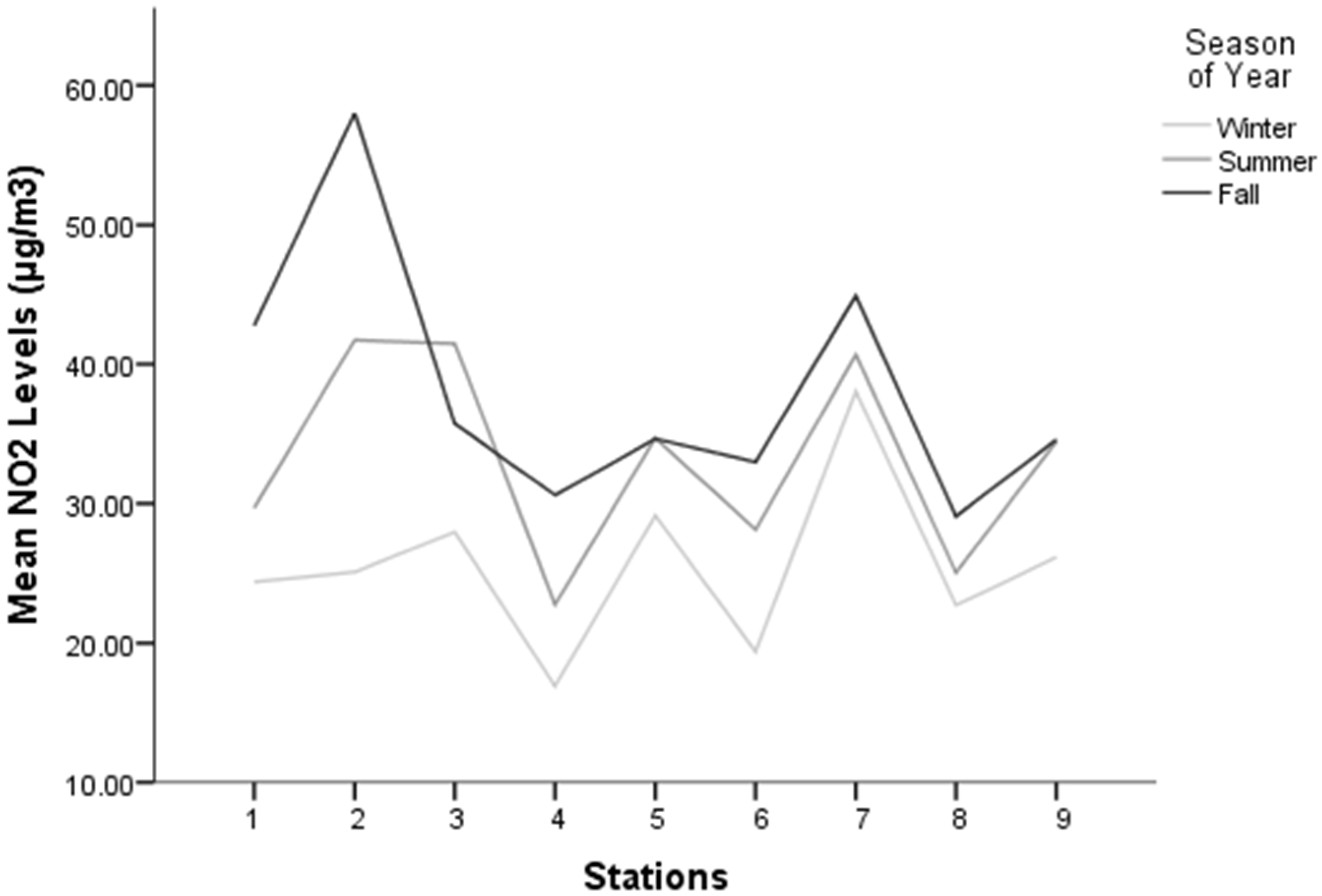
3.2. Spatial and Seasonal Variations of NO2 at Study Locations

The average NO2 levels increased progressively from winter (25.53 μg/m3) to summer (33.19 μg/m3) and fall (38.14 μg/m3) (Table 3). Post hoc analysis showed a significant difference between the winter and fall NO2 concentrations (p = 0.005). Across the study locations, the fall season had a 12.61 μg/m3 higher NO2 concentration than winter. By traffic density, high-traffic areas had an average of 35.79 μg/m3 compared to 25.29 μg/m3 in low-traffic areas, indicating a difference of 10.5 μg/m3, which was statistically significant (p = 0.002).
As shown in Figure 2, the median NO2 concentration increased in both low- and high-traffic areas from winter through summer to fall. NO2 levels were highest in the fall in all locations except at locations 3 and 5, where the summer levels were either higher or the same (Figure 3). Stations 4 (16.89 μg/m3), 6 (19.39 μg/m3), and 8 (22.72 μg/m3) were low-traffic areas, which were reflected in their NO2 concentrations in the winter season. NO2 concentrations in high-traffic areas ranged from 24.4 μg/m3 in the winter at ABC News Stand to 58 μg/m3 in the fall at Golden City Jewelers (Figure 3) (refer also to Table S1). In low-traffic areas, however, the range of NO2 levels was from 16.89 μg/m3 in the winter at Sahan Hair Braiding to 32.99 μg/m3 in the fall at Dove and Matrix Salon. The highest variation in NO2 concentration was seen at location 6 (Dove and Matrix Salon).

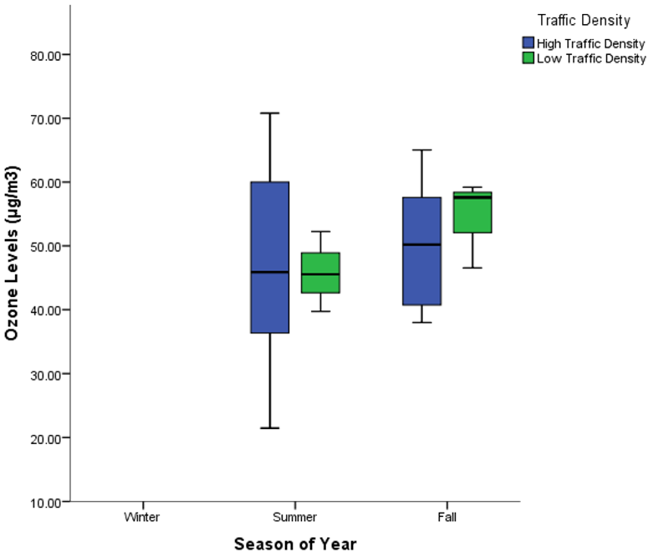
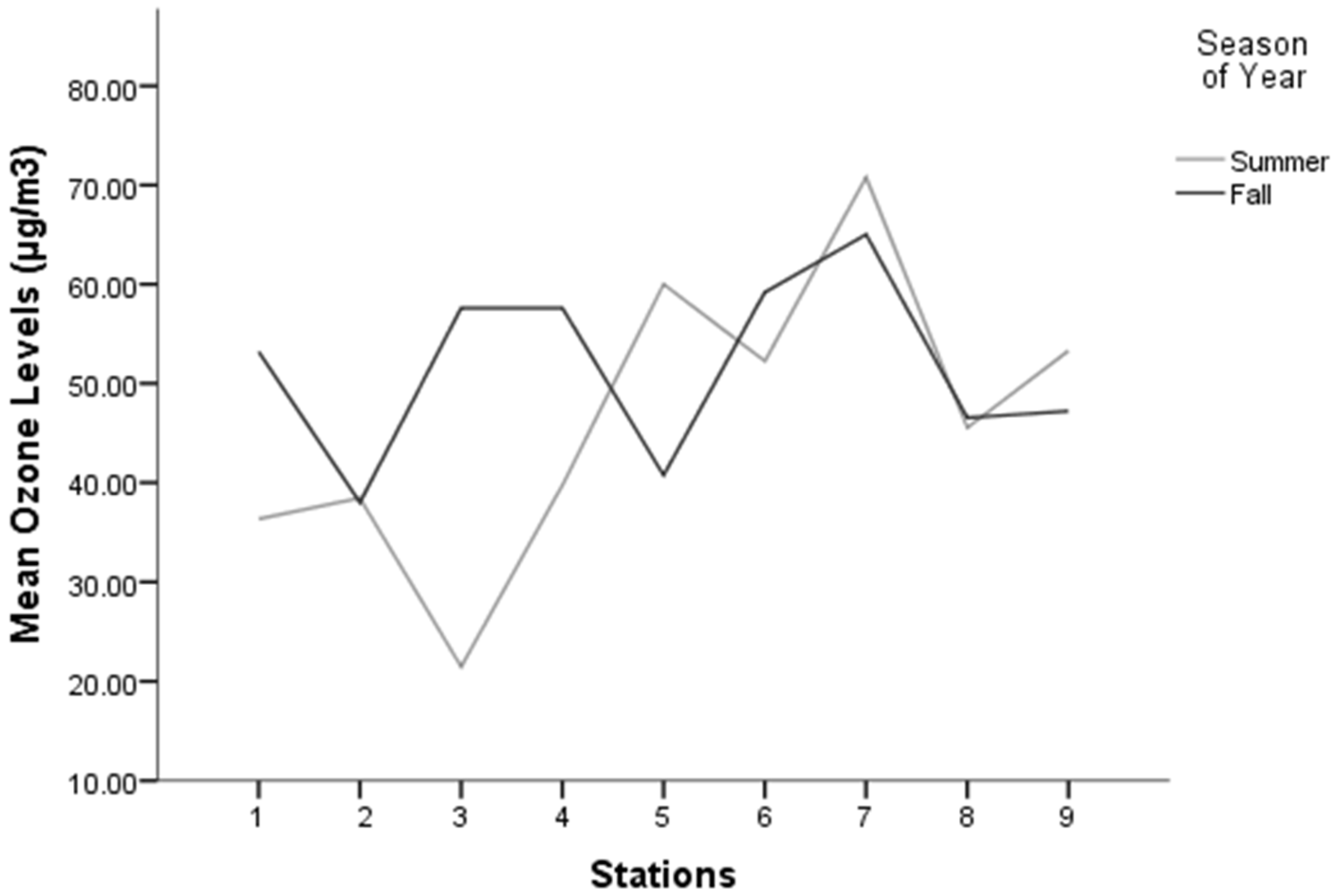
3.3. Spatial and Seasonal Variations of O3 at Study Locations

The mean concentration of O3 was higher in the fall (51.68 μg/m3) compared to the summer (46.43 μg/m3) but was not statistically different (p = 0.37). Low-traffic areas showed higher mean O3 concentrations (50.14 μg/m3) compared with high-traffic areas (48.51 μg/m3) but were not statistically significant (p = 0.79) (Table 4).
O3 concentrations varied by season (Figure 4). These ranged from 21.7 (μg/m3) at the LAZ Parking location during the summer to 70.8 (μg/m3) at Rattan’s Inc. in the fall among the high-traffic locations. At the low-traffic locations, O3 ranged from 39.73 (μg/m3) at the Sahan Hair Braiding site in the summer to 59.2 (μg/m3) at Dove and Matrix Salon in the fall, as shown in Figure 5.
Figure 5 illustrates that O3 levels were higher in the fall than in the summer at locations 1, 3, 4, and 6 but lower in fall than summer levels at locations 5, 7, and 9. Similar measurements were made at sites 2 and 8.
Figure 6 shows a comparison of NO2 and O3 levels during the summer and fall. The trend lines show divergent patterns in NO2 and O3 levels during summer and fall across all study locations. This suggests that as O3 levels increased, NO2 levels decreased. As shown in Figure 6 (and Figure S2), O3 levels were higher than NO2 levels in the summer at locations 1 (ABC News Stand and Coffee Shop, high-traffic), 4 (Sahan Hair Braiding, low-traffic), 5 (Archer Live Poultry, high-traffic), 6 (Dove and Matrix Salon, low-traffic), 7 (Rattan’s Inc., high-traffic), 8 (LI Beauty Supply, low-traffic), and 9 (Wendy’s Restaurant, high-traffic). In the fall, NO2 levels were higher than O3 levels at locations 4 (Sahan Hair Braiding, low-traffic), 5 (Archer Live Poultry, high-traffic), 6 (Dove and Matrix Salon, low-traffic), 7 (Rattan’s Inc., high-traffic), 8 (LI Beauty Supply, low-traffic), and 9 (Wendy’s Restaurant, high-traffic).
The highest O3 levels were recorded at high-traffic locations along main roads. Samples from locations along adjacent LT streets showed comparatively lower concentration levels. Site 7 (Rattan’s Inc.), which is located close to Jamaica Avenue, a high-traffic main road, had the highest O3 levels in the summer (65.03 μg/m3) and in the fall (70.8 μg/m3). This site was also the one with the highest air pollution concentrations overall.

4. Discussion

4.1. Safe Levels of NO2 at Study Locations

When compared with the national ambient air quality standards (NAAQS) threshold or official annual mean NO2 standard of 99.6 μg/m3, the annualized mean for Jamaica Center during the study period was 33.90 μg/m3. Based on the levels calculated, we can infer that the NO2 levels during the two-week period were safe for vendors at Jamaica Center. This does not imply, however, that NO2 levels do not at any time pose a health risk in the study area. Recent studies have shown that even at low concentrations, long-term exposure to traffic-related NO2 can cause ill health and increase the risk of mortality particularly among vulnerable groups [41,42,43]. Seaton et al. [18] found that low levels of NO2 may also contribute to the formation of other pollutants such as O3 and fine particles, leading to increased health risks.

4.2. Spatial and Seasonal Variations of NO2

We found that the levels of NO2 in this study, between 16.89 to 38.05 μg/m3 in winter and from 29.09 to 58 μg/m3 in the fall, were low when compared to previous studies. Our measured NO2 levels over the sampling periods were also lower than the mean levels measured at the nearest continuous air-quality monitoring station in the same year (19.2–58.1 μg/m3) in winter and from 25.6–90.1 μg/m3 in the fall. The same was true for observed summer levels (22.75–41.74 μg/m3) compared to 30.5–82.5 μg/m3 at the continuous air-quality monitoring station. Afif et al. [44] reported average levels of 34.5–110.3 μg/m3, 24.5–177.9 03 μg/m3, and 17.8–96.1 μg/m3 for winter, fall, and summer, respectively. Consistent with Voiculescu et al. [6] and other studies [45,46], we observed the highest NO2 levels in the fall and the lowest in the winter. The lower winter levels of NO2 could be linked to higher wind speeds during the sampling period. In Jamaica Center, the average wind speeds were 41, 37, and 24 miles per hour in winter, fall, and summer, respectively [47], which may account for such a result. Similar findings were reported by other studies that observed “unseasonably low NO2 concentrations coincided with unseasonably high wind speeds” [48]. Additionally, Tang et al. [38] found that windy conditions can influence NO2 concentrations by generating turbulence and reducing diffusion length as air moves over the open end of a diffusion tube.
While NO2 concentrations in the urban environment are influenced by direct emissions from vehicular traffic, meteorological conditions can impede or enhance dispersion in the atmosphere or result in increased pollutant generation. Meteorological effects have been observed by previous studies, including Gorai et al. [19], either directly through physical mechanisms such as the relationship between radiation and O3 or indirectly such as the relationship between high temperatures and low wind speed. In addition to the wind, other factors that can influence NO2 concentrations include temperature, radiation, atmospheric moisture, and mixing depth. Since these factors are inherently linked, their interdependencies or association often make separating their individual effects challenging. Additionally, Niepsch et al. [34] described the effect of topographical features and micro-climatic conditions as well as the urban surrounding such as building density and building heights on air pollution levels [49]. While these features exist in the present study area, an evaluation of the role of such factors in NO2 concentrations was beyond the scope of this study.
The contribution of near-road traffic to NO2 emissions indicates the potential risk to public health. Thus, individuals who spend extended periods near major roads, such as street vendors, are more susceptible to illnesses due to NO2 exposure, as are asthmatics, children, and older adults. According to WHO, NO2 levels within approximately 50 m of heavy traffic maybe 30–100% higher; and short-term NO2 exposures ranging from 30 min to 24 h can cause increased respiratory symptoms and airway inflammation in healthy people as well as emergency room visits and hospital admissions [50]. Although the time resolution of this study was greater than 24 h, previous studies have shown similar results for ambient exposures to NO2, with associated increased respiratory symptoms [51]. Additionally, Niepsch et al. [34] noted that pedestrians and passengers are exposed during periods of high road traffic or commuting times, resulting in high short-term exposure. Residents who live within 300 feet (91.44 m) of a major roadway may be at higher risk for respiratory illnesses, cardiovascular disease, and premature death [52]. As expected in the HT areas in this study, air pollution levels were more pronounced as more emissions were released from moving traffic along major roadways. Additionally, idling vehicles appeared to significantly contribute to higher NO2 levels near heavily trafficked major roads in the study area. Figure 3 and Figure S3 show that in HT areas, there were higher levels of NO2, while the LT areas had lower levels. Each data point in Figure 3 represents the average values at the respective locations.

4.3. Spatial and Seasonal Variations of O3 at Study Locations

The levels of O3 in HT and LT areas during the fall and summer seasons did not show a predictable trend; instead, they fluctuated and were even interchangeable at times. The higher O3 levels in LT areas could have been caused by low wind speeds, resulting in the accumulation and elevated pollution levels at those locations. Wind speed and wind direction were not analyzed in this study; however, Roberts-Semple et al. [9] reported that elevated O3 concentrations resulted mainly from low wind speeds. Additionally, the higher O3 levels at LT sites could have occurred because degradation of O3 occurs in areas with higher levels of NO, as seen in this reaction: NO + O3 → NO2 + O2. Therefore, in areas with less traffic activity, O3 degrades less since there are fewer NO emissions [53]. Austin et al. [54] used k-means clustering to analyze O3 trends concerning characteristic weather patterns and observed the apparent increase in O3 was associated with the photochemistry of locally emitted pollutants rather than regional transported pollutants [54]. They noted that, among the variables, maximum daily temperature and mean daily ground-level wind speed indicate the need for increased O3 controls in the transition months.
As shown in Figure 5 and Figure 6, we observed that O3 levels were higher in the fall than in the summer in all locations except at locations 2 and 8, where there was no change between the seasons. This is not typical, as O3 concentrations are expected to be higher during the summer months, being a secondary air pollutant resulting from photochemical reactions of NOx and VOCs [55]. Since NOx and VOCs were not measured in this study; however, this result is not conclusive. Despite the abundant sunlight during the summer months, previous studies have linked higher O3 levels to higher NOx levels in fall than in summer [10]. Additionally, Yamaji et al. [56] found O3 levels in the summer season to be the lowest of all seasons due to a weak Asian outflow and northward penetration of a marine air mass. We surmise that high wind speeds could also have influenced O3 concentrations in the present study. While meteorological factors could have independently influenced the unusually low O3 summer levels, it is important to note that diffusion tubes could also have limitations in their accuracy and precision. Factors that could significantly impact sampling include the “length of the exposure period, exact location and additional meteorological conditions such as ambient temperature, wind speed and relative humidity”, as observed by Vardoulakis et al. [36] and others [57]. Additionally, micro-climatic conditions at diffusion tube locations and the urban surrounding such as building density and building heights, as observed by Niepsch et al. [34] and Kubota et al. [49], although beyond the scope of this study, as we mentioned under Section 4.2 above, could have influenced NO2 levels. In this study, the limit of detection for NO2 was 20%TEA/water <1.5 ugm−3 or 50%TEA/Acetone <2 ugm−3. Even at levels below Environmental Protection Agency (EPA) standards, however, O3 exposure can pose significant adverse health effects such as an increase in respiratory disorders, with a 0.01 ppm increase in the four-day moving average of maximal eight-hour O3 [58].
One of the major challenges in estimating the potential effects of air pollution exposure in local areas is their distance from regulatory monitoring stations and quantifying the influence of exposure to subsequently estimate health risks. Efforts to estimate health risks to reduce exposure are made more complex by the lack of local datasets. Currently, the finer spatial scale variability in NO2 and air quality in general is lacking in Jamaica Center. In addition, existing monitoring networks have limited spatial coverage and insufficient density to capture small-scale air pollution levels that may vary significantly within a single city, as noted by Apte et al. [23] and Schneider et al. [26]. Therefore, this study addresses two pivotal problems in air quality studies: the cost of air sampling equipment and the distance from regulatory monitoring stations. Previous studies including that by Niepsch et al. [34] have reported findings when the same method/passive diffusion tube sampling was used, with comparable results to studies that obtained data from regulatory monitoring stations. Vardoulakis et al. [36] also reported that the analysis of their results demonstrated very good agreement of NO2 passive samplers with co-located chemiluminescence analyzers, and the O3 diffusion sampler appeared to marginally overestimate the automatic UV analyzer results, particularly in warm-weather periods. Despite some limitations of the diffusion tube method, its validity has been further established by several studies, as discussed below. It is noteworthy that while data obtained in national and regional studies have provided useful data from central monitoring stations, they often present limitations of the real effects of air pollutants, particularly at the local level. This is partly because data collection on such a large scale is cumbersome, and spatial variability due to local meteorology and location is often overlooked [59,60]. Many monitoring networks lack local information, particularly for traffic-generated pollutants known to vary on small scales [61,62]. For such reasons, the diffusion tube sampling method has been used successfully in air-quality studies in addition to the more obvious advantages, including the low cost, handiness, the requirement of no pumps or moving parts, etc. Diffusion tube data can be used in addition to regulatory monitoring station data to enhance the predictive performance of fine-scale NO2 concentrations instead of depending on regulatory monitors alone, which was found in previous studies to cause too much predictive uncertainty [63].
Our approach utilized air sampling at multiple sites, which could potentially yield more representative data that show the unique qualities of the local area. The passive diffusion tubes used in this study are efficient for measuring gas-phase pollutants in various environments as reported by previous studies with similar results, including Niepsch et al. [34], especially as an alternative where conventional approaches to air monitoring at stationary and sparse measurement stations are prohibitively expensive [64]. This approach also identifies pollution hotspots and captures spatial heterogeneity, where average concentrations are particularly low or high [65]. Further, it provides a quick, initial screening tool to identify areas of elevated NO2 for more robust (multiple- or three-tube) monitoring approaches in the future that would account for variability and a more detailed investigation of the potential pollution hotspots. Capturing the data for a longer period may provide a more precise estimate. Despite the limited locations sampled and the single-tube approach, NO2 levels across seasons were associated with heavy traffic density.
Since this pilot study investigated differences in NO2 and O3 levels at adjacent high-traffic versus low-traffic locations over three seasons in a single year, the results may be useful in future studies to predict NO2 concentrations for temporal and seasonal variations across time by comparing data over several years. A primary contribution that our study makes to the current body of air pollution literature is that the differences we observed in NO2 levels between HT and LT traffic sites are significant, and therefore, we suggest that more refined classifications of exposure can be used in future air pollution studies to allow robust conclusions to be drawn concerning public health and epidemiological impacts of air pollutants in Jamaica Center. Further, it demonstrated that diffusion tubes may be used as an alternative to estimate NO2 levels near roadways in urban centers, where data on the variation between corridors with different traffic densities are non-existent, especially when more expensive and more accurate measurements are not available.

5. Conclusions

This study showed that measurements of NO2 and O3 concentrations at a community level are feasible using passive samplers such as diffusion tubes. It also demonstrated the need for emission control policies to reduce NO2 and O3 concentrations in heavily trafficked areas, particularly in the fall and summer seasons. The highest NO2 levels were observed in the fall season, while and highest O3 levels were observed in the summer. High-traffic areas had higher NO2 and O3 levels throughout the seasons. Though the annualized NO2 levels were within the safety margins of the NAAQS, the adverse health impacts of consistent daily exposure should not be ruled out, especially for individuals such as street vendors, who are exposed for prolonged periods during rush hour. Future studies measuring air pollutants using diffusion tubes for longer timeframes within the community and validated against other standardized methods are recommended to better correlate air pollution levels and potential health impacts. More sample locations covered for a longer period may provide better insight into O3 variations, and future co-location studies should apply local bias-adjustment factors, including annual averages, for more accurate and precise calculations of replicate NO2 diffusion tube measurements. Strategies such as green landscaping should be considered to minimize the impact of NO2 and O3 levels.

Supplementary Materials

The following supporting information can be downloaded at: https://www.mdpi.com/article/10.3390/atmos13122042/s1, Figure S1: Study Sites at Jamaica Center; Table S1: NO2 and O3 Measurements in Winter, Fall, and Summer of 2019 in Jamaica Center; Figure S2: Locations and O3 Concentrations in Fall and Spring of 2019; Figure S3: Locations and NO2 Concentrations in Fall, Summer, and Winter of 2019.

Author Contributions

Conceptualization, investigation, writing—original draft preparation, and review and editing to completion, D.R.-S.; literature review, writing, formal analysis, methodology, and formatting, M.G.; methodology, formal analysis, and review and editing to completion, A.A.; GIS maps and visualization, C.A.; validation and review and editing, J.S. All authors have read and agreed to the published version of the manuscript.

Funding

This research was partially funded by the Department of Education STEM—Connect Building a Guided Pathway Grant # 46428-0202.

Institutional Review Board Statement

This study neither involved human subjects nor required identifiable information to be used, studied, analyzed, or generated.

Informed Consent Statement

Not applicable.

Data Availability Statement

Data discussed in this study are contained within the article and Supplementary Material.

Acknowledgments

We thank Yung-Seop Lee for suggesting and exploring possible methods of data analysis. We are also grateful to Michael Griffith, Director of Traffic Planning Studies at the New York City Department of Transportation, for providing valuable information from the Downtown Jamaica Transportation Study.

Conflicts of Interest

The authors declare no conflict of interest. The funders had no role in the design of the study; in the collection, analyses, or interpretation of data; in the writing of the manuscript; or in the decision to publish the results.

References

  1. Ritz, B.; Hoffmann, B.; Peters, A. The Effects of Fine Dust, Ozone, and Nitrogen Dioxide on Health. Dtsch. Arztebl. Int. 2019, 51–52, 881–886. [Google Scholar] [CrossRef] [PubMed]
  2. Luo, K.; Li, R.; Li, W.; Wang, Z.; Ma, X.; Zhang, R.; Fang, X.; Wu, Z.; Cao, Y.; Xu, Q. Acute Effects of Nitrogen Dioxide on Cardiovascular Mortality in Beijing: An Exploration of Spatial Heterogeneity and the District-Specific Predictors. Sci. Rep. 2016, 6, 38328. [Google Scholar] [CrossRef] [PubMed] [Green Version]
  3. Coates, J.; Mar, K.A.; Ojha, N.; Butler, T.M. The Influence of Temperature on Ozone Production under Varying NOx Conditions—A Modelling Study. Atmos. Chem. Phys. 2016, 16, 11601–11615. [Google Scholar] [CrossRef] [Green Version]
  4. Moshammer, H.; Poteser, M.; Kundi, M.; Lemmerer, K.; Weitensfelder, L.; Wallner, P.; Hutter, H.-P. Nitrogen-Dioxide Remains a Valid Air Quality Indicator. Int. J. Environ. Res. Public Health 2020, 17, 3733. [Google Scholar] [CrossRef] [PubMed]
  5. Ban-Weiss, G.A.; McLaughlin, J.P.; Harley, R.A.; Kean, A.J.; Grosjean, E.; Grosjean, D. Carbonyl and Nitrogen Dioxide Emissions from Gasoline- and Diesel-Powered Motor Vehicles. Environ. Sci. Technol. 2008, 42, 3944–3950. [Google Scholar] [CrossRef]
  6. Voiculescu, M.; Constantin, D.-E.; Condurache-Bota, S.; Călmuc, V.; Roșu, A.; Dragomir Bălănică, C.M. Role of Meteorological Parameters in the Diurnal and Seasonal Variation of NO2 in a Romanian Urban Environment. Int. J. Environ. Res. Public Health 2020, 17, 6228. [Google Scholar] [CrossRef] [PubMed]
  7. Pervez, S.; Maruyama, R.; Riaz, A.; Nakai, S. Development of Land Use Regression Model for Seasonal Variation of Nitrogen Dioxide (NO2) in Lahore, Pakistan. Sustainability 2021, 13, 4933. [Google Scholar] [CrossRef]
  8. Romer, P.S.; Duffey, K.C.; Wooldridge, P.J.; Edgerton, E.; Baumann, K.; Feiner, P.A.; Miller, D.O.; Brune, W.H.; Koss, A.R.; De Gouw, J.A.; et al. Effects of Temperature-Dependent NOx Emissions on Continental Ozone Production. Atmos. Chem. Phys. 2018, 18, 2601–2614. [Google Scholar] [CrossRef] [Green Version]
  9. Roberts-Semple, D.; Song, F.; Gao, Y. Seasonal Characteristics of Ambient Nitrogen Oxides and Ground–Level Ozone in Metropolitan Northeastern New Jersey. Atmos. Pollut. Res. 2012, 3, 247–257. [Google Scholar] [CrossRef] [Green Version]
  10. Allen, J. Chemistry in the Sunlight. Earth Observatory. Available online: https://earthobservatory.nasa.gov/features/ChemistrySunlight (accessed on 15 November 2022).
  11. Liu, S.-K.; Cai, S.; Chen, Y.; Xiao, B.; Chen, P.; Xiang, X.-D. The Effect of Pollutional Haze on Pulmonary Function. J. Thorac. Dis. 2016, 8, E41–E56. [Google Scholar] [PubMed]
  12. Jarvis, D.J.; Adamkiewicz, G.; Heroux, M.-E.; Rapp, R.; Kelly, F.J. WHO Guidelines for Indoor Air Quality: Selected Pollutants; WHO: Copenhagen, Denmark, 2010; pp. 201–248. [Google Scholar]
  13. Di, Q.; Amini, H.; Shi, L.; Kloog, I.; Silvern, R.; Kelly, J.; Sabath, M.B.; Choirat, C.; Koutrakis, P.; Lyapustin, A.; et al. Assessing NO2 Concentration and Model Uncertainty with High Spatiotemporal Resolution across the Contiguous United States Using Ensemble Model Averaging. Environ. Sci. Technol. 2020, 54, 1372–1384. [Google Scholar] [CrossRef] [PubMed]
  14. Porter, W.C.; Heald, C.L. The Mechanisms and Meteorological Drivers of the Summertime Ozone–Temperature Relationship. Atmos. Chem. Phys. 2019, 19, 13367–13381. [Google Scholar] [CrossRef] [Green Version]
  15. World Health Organization; Occupational and Environmental Health Team. WHO Air Quality Guidelines for Particulate Matter, Ozone, Nitrogen Dioxide and Sulfur Dioxide: Global Update 2005: Summary of Risk Assessment; World Health Organization: Geneva, Switzerland, 2006. [Google Scholar]
  16. United States Environmental Protection Agency. Ground-Level Ozone Basics. Available online: https://www.epa.gov/ground-level-ozone-pollution/ground-level-ozone-basics (accessed on 19 August 2022).
  17. Manisalidis, I.; Stavropoulou, E.; Stavropoulos, A.; Bezirtzoglou, E. Environmental and Health Impacts of Air Pollution: A Review. Front. Public Health 2020, 8, 14. [Google Scholar] [CrossRef] [PubMed] [Green Version]
  18. Seaton, A. Hypothesis: Ill Health Associated with Low Concentrations of Nitrogen Dioxide—An Effect of Ultrafine Particles? Thorax 2003, 58, 1012–1015. [Google Scholar] [CrossRef] [Green Version]
  19. Gorai, A.K.; Tuluri, F.; Tchounwou, P.B.; Ambinakudige, S. Influence of Local Meteorology and NO2 Conditions on Ground-Level Ozone Concentrations in the Eastern Part of Texas, USA. Air Qual. Atmos. Health 2015, 8, 81–96. [Google Scholar] [CrossRef] [PubMed] [Green Version]
  20. Rowell, A.; Terry, M.E.; Deary, M.E. Comparison of Diffusion Tube–Measured Nitrogen Dioxide Concentrations at Child and Adult Breathing Heights: Who Are We Monitoring for? Air Qual. Atmos. Health 2021, 14, 27–36. [Google Scholar] [CrossRef]
  21. Kirby, C.; Fox, M.; Waterhouse, J. Reliability of Nitrogen Dioxide Passive Diffusion Tubes for Ambient Measurement: In Situ Properties of the Triethanolamine Absorbent. J. Environ. Monit. 2000, 2, 307–312. [Google Scholar] [CrossRef]
  22. Larkin, A.; Hystad, P. Towards Personal Exposures: How Technology Is Changing Air Pollution and Health Research. Curr. Environ. Health Rep. 2017, 4, 463–471. [Google Scholar] [CrossRef]
  23. Apte, J.S.; Messier, K.P.; Gani, S.; Brauer, M.; Kirchstetter, T.W.; Lunden, M.M.; Marshall, J.D.; Portier, C.J.; Vermeulen, R.C.H.; Hamburg, S.P. High-Resolution Air Pollution Mapping with Google Street View Cars: Exploiting Big Data. Environ. Sci. Technol. 2017, 51, 6999–7008. [Google Scholar] [CrossRef]
  24. Brugge, D.; Patton, A.P.; Bob, A.; Reisner, E.; Lowe, L.; Bright, O.-J.M.; Durant, J.L.; Newman, J.; Zamore, W. Developing Community-Level Policy and Practice to Reduce Traffic-Related Air Pollution Exposure. Environ. Justice 2015, 8, 95–104. [Google Scholar] [CrossRef]
  25. U.S. Census Bureau. American Community Survey 1-Year Estimates. Census Reporter Profile Page for NYC-Queens Community District 12—Jamaica, Hollis & St. Albans PUMA, NY. Available online: http://censusreporter.org/profiles/79500US3604112-nyc-queens-community-district-12-jamaica-hollis-st-albans-puma-ny/ (accessed on 15 November 2022).
  26. Schneider, P.; Castell, N.; Vogt, M.; Dauge, F.R.; Lahoz, W.A.; Bartonova, A. Mapping Urban Air Quality in near Real-Time Using Observations from Low-Cost Sensors and Model Information. Environ. Int. 2017, 106, 234–247. [Google Scholar] [CrossRef] [PubMed]
  27. Kendler, S.; Nebenzal, A.; Gold, D.; Reed, P.M.; Fishbain, B. The Effects of Air Pollution Sources/Sensor Array Configurations on the Likelihood of Obtaining Accurate Source Term Estimations. Atmos. Environ. 2021, 246, 117754. [Google Scholar] [CrossRef]
  28. Kanaroglou, P.S.; Jerrett, M.; Morrison, J.; Beckerman, B.; Arain, M.A.; Gilbert, N.L.; Brook, J.R. Establishing an Air Pollution Monitoring Network for Intra-Urban Population Exposure Assessment: A Location-Allocation Approach. Atmos. Environ. 2005, 39, 2399–2409. [Google Scholar] [CrossRef]
  29. Yoshida, I.; Tasaki, Y.; Tomizawa, Y. Optimal Placement of Sampling Locations for Identification of a Two-Dimensional Space. Georisk Assess. Manag. Risk Eng. Syst. Geohazards 2022, 16, 98–113. [Google Scholar] [CrossRef]
  30. Mano, Z.; Kendler, S.; Fishbain, B. Information Theory Solution Approach to the Air Pollution Sensor Location-Allocation Problem. Sensors 2022, 22, 3808. [Google Scholar] [CrossRef]
  31. New York City Department of Transportation. Queens Village/Jamaica Avenue Transportation Study: Final Report (Report Number: P.I.N. PTDT14D00.G05); New York City Department of Transportation: New York, NY, USA, 2015. [Google Scholar]
  32. New York City Department of Transportation. Downtown Jamaica Transportation Study Final Report. (Report Number: PIN PTDT18D00.G12). Available online: https://www.nyc.gov.downtown-jamaica-study-final-report.pdf (accessed on 28 November 2022).
  33. Practical Guidance: NO2 Diffusion Tubes for LAQM. Gov.uk. Available online: https://laqm.defra.gov.uk/air-quality/air-quality-assessment/practical-guidance/ (accessed on 1 December 2022).
  34. Niepsch, D.; Clarke, L.J.; Tzoulas, K.; Cavan, G. Spatiotemporal Variability of Nitrogen Dioxide (NO2) Pollution in Manchester (UK) City Centre (2017–2018) Using a Fine Spatial Scale Single-NOx Diffusion Tube Network. Environ. Geochem. Health 2022, 44, 3907–3927. [Google Scholar] [CrossRef]
  35. Air Quality Guide for Nitrogen Dioxide Air Quality Index Protect Your Health near Roadways. Airnow.gov. Available online: https://www.airnow.gov/sites/default/files/2018-06/no2.pdf (accessed on 10 August 2022).
  36. Vardoulakis, S.; Lumbreras, J.; Solazzo, E. Comparative Evaluation of Nitrogen Oxides and Ozone Passive Diffusion Tubes for Exposure Studies. Atmos. Environ. 2009, 43, 2509–2517. [Google Scholar] [CrossRef]
  37. Varshney, C.K.; Singh, A.P. Passive Samplers for NOx Monitoring: A Critical Review. Environmentalist 2003, 23, 127–136. [Google Scholar] [CrossRef]
  38. Tang, Y.S.; Cape, J.N.; Sutton, M.A. Development and Types of Passive Samplers for Monitoring Atmospheric NO2 and NH3 Concentrations. Sci. World J. 2001, 1, 513–529. [Google Scholar] [CrossRef] [Green Version]
  39. Nash, D.G.; Leith, D. Use of Passive Diffusion Tubes to Monitor Air Pollutants. J. Air Waste Manag. Assoc. 2010, 60, 204–209. [Google Scholar] [CrossRef]
  40. United States Environmental Protection Agency. NAAQS Table 2014. Available online: https://www.epa.gov/criteria-air-pollutants/naaqs-table (accessed on 10 August 2022).
  41. Yazdi, M.D.; Wang, Y.; Di, Q.; Requia, W.J.; Wei, Y.; Shi, L.; Sabath, M.B.; Dominici, F.; Coull, B.; Evans, J.S.; et al. Long-Term Effect of Exposure to Lower Concentrations of Air Pollution on Mortality among US Medicare Participants and Vulnerable Subgroups: A Doubly-Robust Approach. Lancet Planet. Health 2021, 5, e689–e697. [Google Scholar] [CrossRef] [PubMed]
  42. Samoli, E.; Aga, E.; Touloumi, G.; Nisiotis, K.; Forsberg, B.; Lefranc, A.; Pekkanen, J.; Wojtyniak, B.; Schindler, C.; Niciu, E.; et al. Short-Term Effects of Nitrogen Dioxide on Mortality: An Analysis within the APHEA Project. Eur. Respir. J. 2006, 27, 1129–1138. [Google Scholar] [CrossRef] [PubMed]
  43. Chiusolo, M.; Cadum, E.; Stafoggia, M.; Galassi, C.; Berti, G.; Faustini, A.; Bisanti, L.; Vigotti, M.A.; Dessì, M.P.; Cernigliaro, A.; et al. Short-Term Effects of Nitrogen Dioxide on Mortality and Susceptibility Factors in 10 Italian Cities: The EpiAir Study. Environ. Health Perspect. 2011, 119, 1233–1238. [Google Scholar] [CrossRef] [PubMed] [Green Version]
  44. Afif, C.; Dutot, A.L.; Jambert, C.; Abboud, M.; Adjizian-Gérard, J.; Farah, W.; Perros, P.E.; Rizk, T. Statistical Approach for the Characterization of NO2 Concentrations in Beirut. Air Qual. Atmos. Health 2009, 2, 57–67. [Google Scholar] [CrossRef] [Green Version]
  45. Perkauskas, D.; Mikelinskiene, A. Evaluation of SO2 and NO2 Concentration Levels in Vilnius (Lithuania) Using Passive Diffusion Samplers. Environ. Pollut. 1998, 102, 249–252. [Google Scholar] [CrossRef]
  46. Mavroidis, I.; Ilia, M. Trends of NOx, NO2 and O3 Concentrations at Three Different Types of Air Quality Monitoring Stations in Athens, Greece. Atmos. Environ. 2012, 63, 135–147. [Google Scholar] [CrossRef]
  47. New York City. NY Weather History. Wunderground.com. Available online: https://www.wunderground.com/history/monthly/us/ny/new-york-city (accessed on 2 August 2022).
  48. Hargreaves, P.R.; Leidi, A.; Grubb, H.J.; Howe, M.T.; Mugglestone, M.A. Local and Seasonal Variations in Atmospheric Nitrogen Dioxide Levels at Rothamsted, UK, and Relationships with Meteorological Conditions. Atmos. Environ. 2000, 34, 843–853. [Google Scholar] [CrossRef]
  49. Kubota, T.; Miura, M.; Tominaga, Y.; Mochida, A. Wind Tunnel Tests on the Relationship between Building Density and Pedestrian-Level Wind Velocity: Development of Guidelines for Realizing Acceptable Wind Environment in Residential Neighborhoods. Build. Environ. 2008, 43, 1699–1708. [Google Scholar] [CrossRef]
  50. WHO Regional Office for Europe: Europe, UK. Proximity to Roads, NO2, Other Air Pollutants and Their Mixtures; WHO Regional Office for Europe: Copenhagen, Denmark, 2013. [Google Scholar]
  51. Grange, S.K.; Lewis, A.C.; Moller, S.J.; Carslaw, D.C. Lower Vehicular Primary Emissions of NO2 in Europe than Assumed in Policy Projections. Nat. Geosci. 2017, 10, 914–918. [Google Scholar] [CrossRef]
  52. How Does Transportation Impact Health? RWJF. Available online: https://www.rwjf.org/en/library/research/2012/10/how-does-transportation-impact-health-.html (accessed on 2 August 2022).
  53. Why Are Ozone Concentrations Higher in Rural Areas than in Cities? Irceline.Be. Available online: https://www.Irceline.Be/En/Documentation/Faq/Why-Are-Ozone-Concentrations-Higher-in-Rural-Areas-than-in-Cities (accessed on 13 June 2022).
  54. Austin, E.; Zanobetti, A.; Coull, B.; Schwartz, J.; Gold, D.R.; Koutrakis, P. Ozone Trends and Their Relationship to Characteristic Weather Patterns. J. Expo. Sci. Environ. Epidemiol. 2015, 25, 532–542. [Google Scholar] [CrossRef]
  55. Simon, H.; Reff, A.; Wells, B.; Xing, J.; Frank, N. Ozone Trends across the United States over a Period of Decreasing NOx and VOC Emissions. Environ. Sci. Technol. 2015, 49, 186–195. [Google Scholar] [CrossRef] [PubMed] [Green Version]
  56. Yamaji, K.; Ohara, T.; Uno, I.; Tanimoto, H.; Kurokawa, J.; Akimoto, H. Analysis of the Seasonal Variation of Ozone in the Boundary Layer in East Asia Using the Community Multi-Scale Air Quality Model: What Controls Surface Ozone Levels over Japan? Atmos. Environ 1994, 40, 1856–1868. [Google Scholar] [CrossRef]
  57. Cape, J.N. The Use of Passive Diffusion Tubes for Measuring Concentrations of Nitrogen Dioxide in Air. Crit. Rev. Anal. Chem. 2009, 39, 289–310. [Google Scholar] [CrossRef] [Green Version]
  58. Ren, C.; Melly, S.; Schwartz, J. Modifiers of Short-Term Effects of Ozone on Mortality in Eastern Massachusetts—A Casecrossover Analysis at Individual Level. Environ. Health 2010, 9, 3. [Google Scholar] [CrossRef] [PubMed] [Green Version]
  59. Forastiere, F.; Stafoggia, M.; Picciotto, S.; Bellander, T.; D’Ippoliti, D.; Lanki, T.; von Klot, S.; Nyberg, F.; Paatero, P.; Peters, A.; et al. A Case-Crossover Analysis of out-of-Hospital Coronary Deaths and Air Pollution in Rome, Italy. Am. J. Respir. Crit. Care Med. 2005, 172, 1549–1555. [Google Scholar] [CrossRef]
  60. Varadarajan, C. Development of a Source-Meteorology-Receptor (SMR) Approach Using Fine Particulate Intermittent Monitored Concentration Data for Urban Areas in Ohio; University of Toledo: Toledo, OH, USA, 2007. [Google Scholar]
  61. Kan, H.; Chen, B.; Zhao, N.; London, S.J.; Song, G.; Chen, G. Part 1. A Timeseries Study of Ambient Air Pollution and Daily Mortality in Shanghai, China. Res. Rep. Health Eff. Inst. 2010, 1, 17–78. [Google Scholar]
  62. Giles, L.V.; Barn, P.; Künzli, N.; Romieu, I.; Mittleman, M.A.; van Eeden, S.; Allen, R.; Carlsten, C.; Stieb, D.; Noonan, C.; et al. From Good Intentions to Proven Interventions: Effectiveness of Actions to Reduce the Health Impacts of Air Pollution. Environ. Health Perspect. 2011, 119, 29–36. [Google Scholar] [CrossRef] [Green Version]
  63. Pannullo, F.; Lee, D.; Waclawski, E.; Leyland, A.H. Improving Spatial Nitrogen Dioxide Prediction Using Diffusion Tubes: A Case Study in West Central Scotland. Atmos. Environ. 2015, 118, 227–235. [Google Scholar] [CrossRef] [Green Version]
  64. Cox, R.M. The Use of Passive Sampling to Monitor Forest Exposure to O3, NO2 and SO2: A Review and Some Case Studies. Environ. Pollut. 2003, 126, 301–311. [Google Scholar] [CrossRef]
  65. Kumar, P.; Morawska, L.; Martani, C.; Biskos, G.; Neophytou, M.; Di Sabatino, S.; Bell, M.; Norford, L.; Britter, R. The Rise of Low-Cost Sensing for Managing Air Pollution in Cities. Environ. Int. 2015, 75, 199–205. [Google Scholar] [CrossRef]
Figure 1. Jamaica Center-Parsons-Archer transportation hub.
Atmosphere 13 02042 g001
Figure 2. Variations in NO2 concentrations (median) by traffic density across the three seasons.
Atmosphere 13 02042 g002
Figure 3. Nitrogen dioxide levels in winter, fall, and summer at Jamaica Center in 2019. Key: (1) ABC Newsstand Coffee Shop—HT; (2) Golden City Jeweler’s—HT; (3) LAZ Parking—HT; (4) Sahan Hair Braiding—LT; (5) Archer Live Poultry—HT; (6) Dove and Matrix Salon—LT; (7) Rattan’s Inc.—HT; (8) Long Island Beauty Supply—LT; (9) Wendy’s Restaurant—HT. HT, high traffic; LT, low traffic.
Atmosphere 13 02042 g003
Figure 4. Variations in O3 concentrations (median) by traffic density during fall and summer.
Atmosphere 13 02042 g004
Figure 5. O3 concentration for fall and summer 2019 at study locations.
Atmosphere 13 02042 g005
Figure 6. NO2 and O3 concentrations across the study centers. Fall season on the left and summer season on the right.
Atmosphere 13 02042 g006
Table 1. Description of Sample Locations.
SiteSite Name/DescriptionTraffic
Density
LatitudeLongitude
1ABC News Stand/Coffee ShopHigh40.702854−73.799294
2Golden City JewelersHigh40.703752−73.799481
3LAZ ParkingHigh40.703132−73.798622
4Sahan Hair BraidingLow40.70326−73.791721
5Archer Live PoultryHigh40.703892−73.793863
6Dove and Matrix SalonLow40.705061−73.794406
7Rattan’s Inc.High40.704848−73.795427
8Long Island Beauty SupplyLow40.704433−73.799348
9Wendy’s RestaurantHigh40.703442−73.800393
Table 2. NO2 Annualized Data.
Start DateEnd DateB1D1BD1
17 January 20194 February 201973.4725.5373.47
4 February 20199 July 201962.34--
9 July 20192 August 201953.0833.1953.08
2 August 20192 October 201955.69--
2 October 201918 October 201938.2538.1438.25
18 October 201931 December 201963.22--
Average annual mean (average of B1) = 57.68. Measured mean (average of D1) = 32.29. Period mean (average of BD1 = 54.93. Key: B1, background NO2 concentrations from EPA continuous monitoring data for 2019 at Queens College; D1, directly measured NO2 concentrations in this study using diffusion tubes at selected sites in Jamaica Center for two-week periods during the spring, summer, and fall of 2019; BD1, NO2 concentrations from EPA data for periods when NO2 concentrations were directly measured in this study using diffusion tubes (for a fair comparison to annual continuously measured data). Start and end dates, B1 corresponding periods when NO2 concentrations were directly measured in the present study; annualization ratio: annual mean/period mean (57.68 μg/m3/54.93 μg/m3 = 1.05); annualized NO2 concentration: 1.05 × 32.29 μg/m3 = 33.9 μg/m3.
Table 3. Comparison of NO2 Variation by Season and Traffic Density.
Winter
Mean (95%CI)
Summer
Mean (95%CI)
Fall
Mean (95%CI)
Total (95%CI)p-Value
NO2 (μg/m3)25.53 (20.84–30.22)33.19 (27.65–38.72)38.14 (31.18–45.11)32.29 (28.74–35.84)0.006
High-Traffic Mean (95%CI)Low-Traffic Mean (95%CI)Mean Difference (95%CI)p-value
NO2 (μg/m3)35.79 (32.81–38.77)25.29 (11.73- 28.85)10.497 (4.12–16.87)0.002
Key: NO2, nitrogen dioxide; μg/m3, microgram per cubic meter; 95%CI, 95% confidence interval; winter vs. fall (p = 0.00).
Table 4. Comparison of O3 Variation by Season and Traffic Density.
Fall
Mean (95%CI)
Summer
Mean (95%CI)
Total (95%CI)p-Value
O3 (μg/m3)51.68 (44.70–58.67) 46.43 (35.25–57.61)49.06 (43.05–55.09)0.372
High-Traffic Mean (95%CI)Low-Traffic Mean (95%CI)Mean Difference (95%CI)p-value
O3 (μg/m3)48.51 (40.39–56.63)50.14 (43.98–56.30)−1.63 (−14.79–11.53)0.79
Key: O3, ozone; μg/m3, microgram per cubic meter; 95%CI, 95% confidence interval.
Publisher’s Note: MDPI stays neutral with regard to jurisdictional claims in published maps and institutional affiliations.

