1. Introduction
Mid-latitude sporadic-E (commonly written as ‘Es’) is an intermittent phenomenon of the E region of the ionosphere, consisting of thin, transient, and patchy layers of intense ionization, with electron densities frequently much higher than those in the background ionosphere.
Because of its enhanced ionization density, sporadic-E can adversely affect a wide range of radio communications and radar systems, particularly those where the angle between the incident radio signal and the sporadic-E layer is very oblique [
1]. Es can also cause scintillation on low-elevation satellite signals, including GNSS [
2].
The mid-latitude form of sporadic-E [
3,
4,
5,
6], which is the focus of this study, consists of regions of high ionization at altitudes of 90–130 km [
5,
7,
8] in thin layers up to a few km thick [
9,
10] and with horizontal extent typically between a few km and a few hundred km [
11]. The enhanced ionization density within Es clouds is caused by concentrations of long-lived metallic ions, ablated from meteors, and their associated free electrons [
8,
10,
12]. Ions and neutrals are strongly coupled in the lower E region and there is a high degree of correlation between the occurrence of Es and the presence of sporadic metal layers [
13,
14,
15].
Collisional coupling with neutrals causes the metal ions to be strongly affected by neutral winds. The wind shear theory [
16,
17] is widely accepted as describing the principal mechanism behind mid-latitude Es-layer formation, by which vertical gradients in the zonal wind concentrate the metal ions into narrow height ranges [
5,
18] through Lorentz forces. Observations that directly support this theory have recently come from a number of GNSS radio occultation and ionosonde studies e.g., [
19,
20]. For a more comprehensive overview of the characteristics of sporadic-E, see our earlier article [
21], Section II and references therein.
Sporadic-E clouds regularly support oblique reflection of radio signals in the high frequency (HF) and very high frequency (VHF) ranges, up to at least 160 MHz [
22]—see
Figure 1. Although there is a clear consensus about the principal mechanisms of formation of sporadic-E, the process by which oblique VHF radio wave reflection from Es clouds occurs has never been clearly established. Authors have variously described it as specular reflection [
23,
24], scattering [
23,
25], or magnetoionic double refraction [
26]. Each of these mechanisms will affect the polarization of the reflected signal differently, as discussed in
Section 4.1.
The ionosphere consists of a partially ionized plasma in the presence of the Earth’s magnetic field. It can be shown from the Appleton-Hartree equation [
27,
28], which describes the relationship between the phase refractive index along the path of an electromagnetic wave and the local properties of the magnetized plasma, that only two wave modes, known as ‘characteristic modes’, can propagate. A linearly polarized wave entering the ionosphere must couple into a combination of the two characteristic modes.
The polarization of each of the characteristic modes can be represented by the quantity R, the complex ratio of two orthogonal linear components of the field strength [
28] (pp. 8–20):
where
X =
ωN2/
ω2,
Y =
ωB/
ω,
YL =
ωL/
ω,
YT =
ωT/
ω,
Z =
ν/
ω.
In (1), ωN is the plasma frequency (the natural frequency of charge displacement), ωB is the electron gyro frequency (the natural frequency at which electrons rotate around the magnetic lines of force), ωL and ωT are the longitudinal and transverse components of ωB relative to the direction of propagation, and ν is the electron collision frequency. YL and YT are the magnetic terms and Z is the absorption term.
The two solutions of (1) correspond to the two characteristic modes, known as the ‘ordinary’ (O) and ‘extraordinary’ (X) waves, which are in general elliptically polarized and have opposite senses of rotation. Because the refractive index in the plasma for each of the modes is different and depends on local plasma and magnetic field conditions, the O and X waves travel at different velocities and can follow significantly different paths. Note that the maximum usable frequency (MUF) on any given path is higher for the X mode than for the O mode, so that close to the MUF only the X mode may sometimes be reflected [
29].
In the general case where both O and X modes are present on exiting the ionosphere, the resulting combined wave is elliptically polarized, with ellipticity and tilt angle depending on the amplitude, orientation, and phase relationship between the O and X waves at that point. The polarization of the wave reaching the receiver via magnetoionic double refraction can therefore be very different from that of the originally transmitted wave, and can vary significantly as the relationship between the O and X modes changes.
Several experimental studies of the polarization of VHF signals after oblique Es reflection have been described in the literature [
30,
31], although they give only limited information about the polarization state of the reflected wave. One study, however [
32], reports more detailed observations of Es reflections from a single 55 MHz television transmitter over an 1160 km path. The results indicate that the received polarization was mainly elliptical, and that the major axis of the ellipse deviated significantly from the horizontal polarization of the transmitted signal.
Our own earlier work [
21] describes a novel system for making radio wave polarization measurements of sporadic-E signals at 50 MHz, with higher temporal resolution and more accurately than has previously been possible. That article also presents an analysis of two case study recordings to prove the performance of the technique; for these two specific examples, received signals were clearly elliptically polarized rather than linearly polarized.
The current article reports the results of a polarization measurement campaign in the summer of 2018. The campaign gathered a large amount of data at a receiving station in the south of the UK using six European amateur radio beacon transmitters, received via sporadic-E reflection, as 50 MHz signal sources. In
Section 2, an overview of the measurement system is given, the scope of the measurement campaign is defined, and the data analysis approach is described.
Section 3 describes the distribution of polarization parameters observed across all six beacons, plus a more detailed examination of the results for two similar propagation paths between which consistently differing signal polarization was observed. In
Section 4, the results are discussed in the context of investigating the true nature of the reflection process, and outstanding issues are identified. Finally, in
Section 5, conclusions are presented and opportunities for further work described.
2. Materials and Methods
2.1. Polarization Measurement System
Our measurement system uses modern software-defined radio (SDR) techniques, which allow much higher cadence and more accurate measurement of the polarization parameters of received signals than has previously been possible. Care is taken to reduce environmental electromagnetic noise and to account for ground reflection effects. A summary of the approach is given here but we refer to our earlier article [
21] for complete details, including equipment calibration, the minimization and compensation of environmental factors including ground reflection, and the estimated uncertainty in the measurements.
The measurement system consists of a pair of identical directional antennas, one oriented for horizontal polarization and the other for vertical polarization. The two antennas separately feed a dual channel, directly digitizing receiver, with its associated signal processing and data storage capability. See
Figure 2.
The two antennas are of a seven-element loop-fed (LFA) Yagi-Uda design and are interleaved orthogonally on the same boom. The LFA design was chosen because it has low gain for signals from the side and rear of the antenna; this is particularly important for the reduction of man-made electromagnetic noise, which typically dominates natural noise at 50 MHz at the receiving location. The antennas were mounted at a height of 18 m above the ground in order to minimise environmental near-field effects, to further reduce the impact of local noise, and to maximize antenna gain at low elevation angles.
The dual receiver, an Apache Labs ANAN-8000DLE, digitally samples the two antenna inputs directly at the 50 MHz beacon frequency. The digital data stream is then filtered and down-sampled to produce four 16-bit data streams characterizing the in-phase and quadrature (IQ) components of the two sampled antenna voltages. These are then filtered further, to produce a narrow-band data stream (normally 6000 samples per second) which is stored on hard disk for post-processing. For calibration purposes, a stable comparison signal is manually switched to the two receivers at the beginning and/or end of each recording period.
In the post-processing stage, which is described in detail in [
21], a single complex amplitude is calculated from each pair of I and Q samples. This data stream is then examined to identify the useful time segment(s) of the recording, to determine the precise frequencies of the beacon and calibration signals, and to identify a clear frequency for ambient noise level measurement. This information is used to extract beacon, calibration, and noise data streams for the desired time segment, each filtered to a 25 Hz bandwidth.
The calibration signal is used to derive correction factors to compensate for receiver offsets and drift, including differential amplitude, differential phase, and absolute power. These correction factors are then applied to the filtered beacon data streams, along with static corrections for differential antenna cable loss and phase lag. The effect of the ground reflection in front of the antenna is also compensated for.
The beacon data streams are then cleaned by removing samples which are less than 10 dB above the average ambient noise level on each channel and by using a ‘dynamic squelch’ to remove as much as possible of the beacon’s periodic morse code identification message.
Finally, per-sample polarization parameters are calculated from the filtered, calibrated, and cleaned data. The power ratio and the phase difference between the vertically and horizontally polarized signals are directly measured; from them, the full polarization characteristics of the wave can be calculated.
2.2. Signal Sources
Six European amateur radio 50 MHz beacon transmitters were used as signal sources. These beacons operate at frequencies between 50.4 MHz and 50.5 MHz, continuously transmitting narrow-band signals on a 24-h basis. Power output is low, typically 1–10 W, and antennas are normally omnidirectional and linearly polarized. The beacons transmit a continuous carrier plus a periodic station identification in Morse code.
The great circle paths from the beacons to our measurement location at Churt in the south of England (51.135 N, 0.784 W) were over distances between 1100 km and 1650 km, and over a range of orientations to the Earth’s magnetic field—see
Figure 3. The minimum great circle distance was selected to reduce the possibility that other propagation modes (such as tropospheric ducting) were present. The maximum distance was chosen to reduce the likelihood of double-hop Es propagation with an intermediate ground reflection, so that the likely reflection zone, close to the path midpoint, can more easily be identified. Note that in western Europe, magnetic North is within a few degrees of geographical North.
Table 1 lists the parameters of the beacons observed for this study, showing for each beacon its location, the great circle distance from the beacon to the receiver, the great circle azimuth (bearing) from the beacon to the receiver, its transmission frequency, and its antenna polarization.
2.3. Characterization of Polarization State
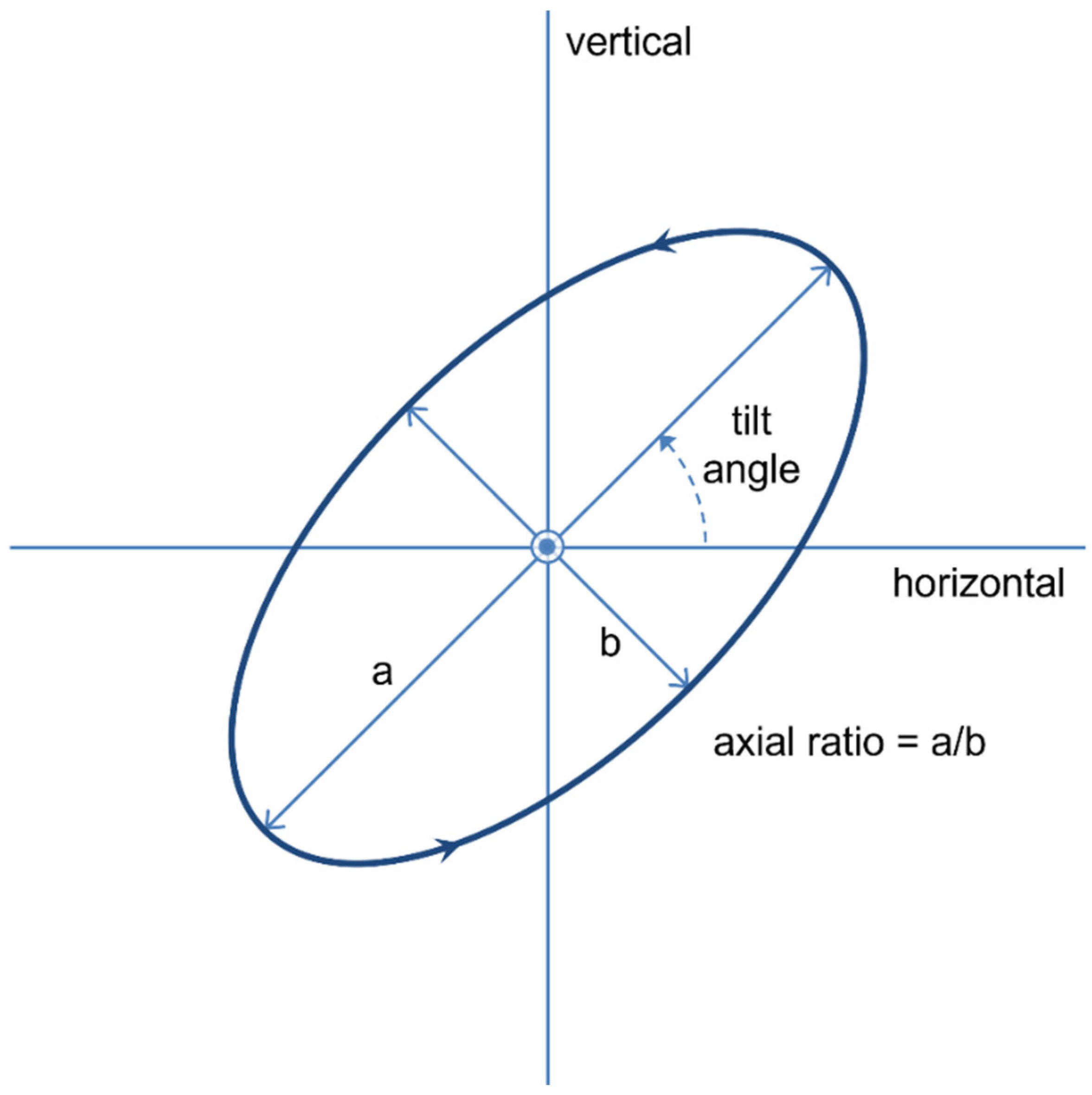
Linear and circular polarization are both special cases of the general form—elliptical polarization. As shown in
Figure 4, the shape and orientation of the polarization ellipse can be characterized by its axial ratio, defined as the ratio of the major axis to the minor axis, and its tilt angle, measured clockwise to the major axis from the horizontal. A pure circularly polarized wave has an axial ratio of 1, and a pure linearly polarized wave has an axial ratio of infinity. All other values of axial ratio correspond to elliptical polarization.
Note that the IEEE standard definitions [
33,
34] of these parameters are adopted in this article, according to which both the sense of rotation of the ellipse and the tilt angle are defined looking along the direction of travel of the wave away from the transmitter. The axial ratio is defined to be positive when the sense of rotation is right-handed, and negative when the sense of rotation is left-handed.
Following the IEEE conventions, it can be shown [
34,
35] that, for the axial ratio
ar and tilt angle
τ of the polarization ellipse [
21]:
where
P is the ratio of the vertical field strength to the horizontal field strength and
φ is the phase difference between the two fields. Tilt angle
τ is defined to be in the range ±90°.
Using the polarization measurement system described in
Section 2.1, and for a polarization state typical of observations reported in this article, the per-sample expanded standard uncertainty (95% confidence) in axial ratio is estimated to be 1.3, and in tilt angle 4.3° [
21].
For some purposes, a more useful way to represent the polarization state of an electromagnetic wave is the Poincaré Sphere [
35,
36,
37,
38], in which key polarization characteristics are plotted on the surface of a unit sphere using a normalized, three-dimensional, spherical coordinate system. Each possible polarization state maps uniquely to a point on the surface of the sphere—see
Figure 5.
On the surface of the sphere, the ‘longitude’ is twice the tilt angle τ as defined in (3) and (4), and the ‘latitude’ is twice the ellipticity angle ε, which is related to the axial ratio by [
36]:
It follows that the ‘North Pole’ of the Poincaré Sphere maps to pure left-hand circular polarization and the ‘South Pole’ maps to pure right-hand circular polarization. The ‘Equator’ maps to linear polarization, with pure horizontal at 0° ‘longitude’, pure vertical at 180° ‘longitude’, and other linear orientations around the equator line. Away from the ‘Equator’ and the poles, polarization states in the ‘Northern Hemisphere’ are left-hand elliptically polarized, and in the ‘Southern Hemisphere’, right-hand elliptically polarized.
The Poincaré Sphere gives a straightforward visual representation of the polarization state and has several useful features. Particularly relevant to this study is that a sequence of states can be plotted on the surface of the sphere, to reveal how the polarization of a signal changes over time. In addition, the Poincaré Sphere can clearly reveal complete or partial depolarization. While a fully polarized wave will always appear to be on the surface of the sphere, a partially polarized wave will appear to be inside the sphere and a completely unpolarized wave will be at the center [
39].
3. Results
Sporadic-E is an intermittent phenomenon which is very localized and difficult to predict, meaning that an opportunistic approach must be taken if a useful amount of data is to be gathered. There is a strong maximum in the incidence of Es in the hemispheric summer [
30,
40,
41], so the period from May to August was chosen for the measurement campaign in 2018. The polarization measurement system described in
Section 2.1 was used to gather a large amount of data at a receiving station in the south of the UK, using six European amateur radio beacon transmitters as sources, as described in
Section 2.2.
The measurement campaign was in two parts. In the first part, a general survey was conducted, focused on gathering data from as many sources as possible over great circle paths at a range of distances, and orientations to the Earth’s magnetic field. The aim of this work was to establish the general nature of the received polarization, and specifically whether it was normally elliptical or linear, in order to throw light on the nature of reflection from sporadic-E. The results of this part of the study are described in
Section 3.1.
The second part of the study focused on a more in-depth study of the signals from Slovenia and Hungary. These two great circle paths are close to each other, and each is roughly perpendicular to the Earth’s magnetic field at the estimated point of reflection. Repeated measurements were made over multiple days. The results of this phase are reported in
Section 3.2.
Note that the pragmatic definition adopted here of a sporadic-E ‘reflection event’ is that the Es ionization density became high enough to obliquely reflect 50 MHz radio waves for a period of time. Where two ‘reflection events’ are close to each other in time and location, it may be possible to infer that they are produced by the same Es cloud, but in general Es is so variable and transient that the reflection events must be considered to be distinct.
3.1. General Survey Results
The survey element of the campaign gathered data from all six signal sources, as shown in
Table 2. The volume of data is not uniform across sources because of the sporadic nature of Es, but there is enough to clearly identify polarization behaviour in each case. A total of 214.3 min of calibrated and cleaned data was analyzed across 15 sporadic-E reflection events, with two of them potentially relating to the same Es cloud—see
Section 3.2.
Note that, during typical sporadic-E reflection events, the strength of the received signal is frequently highly variable. Where the signal strength of either the horizontally or the vertically polarized component falls below an acceptable level of signal to noise ratio, measurements are deliberately omitted from the analyzed data so that polarization parameters are not calculated on noise. In this event, the total duration of calibrated and cleaned data may be less than the overall recorded length of the reflection event.
In order to establish an overall picture of polarization behaviour,
Figure 6,
Figure 7,
Figure 8,
Figure 9,
Figure 10 and
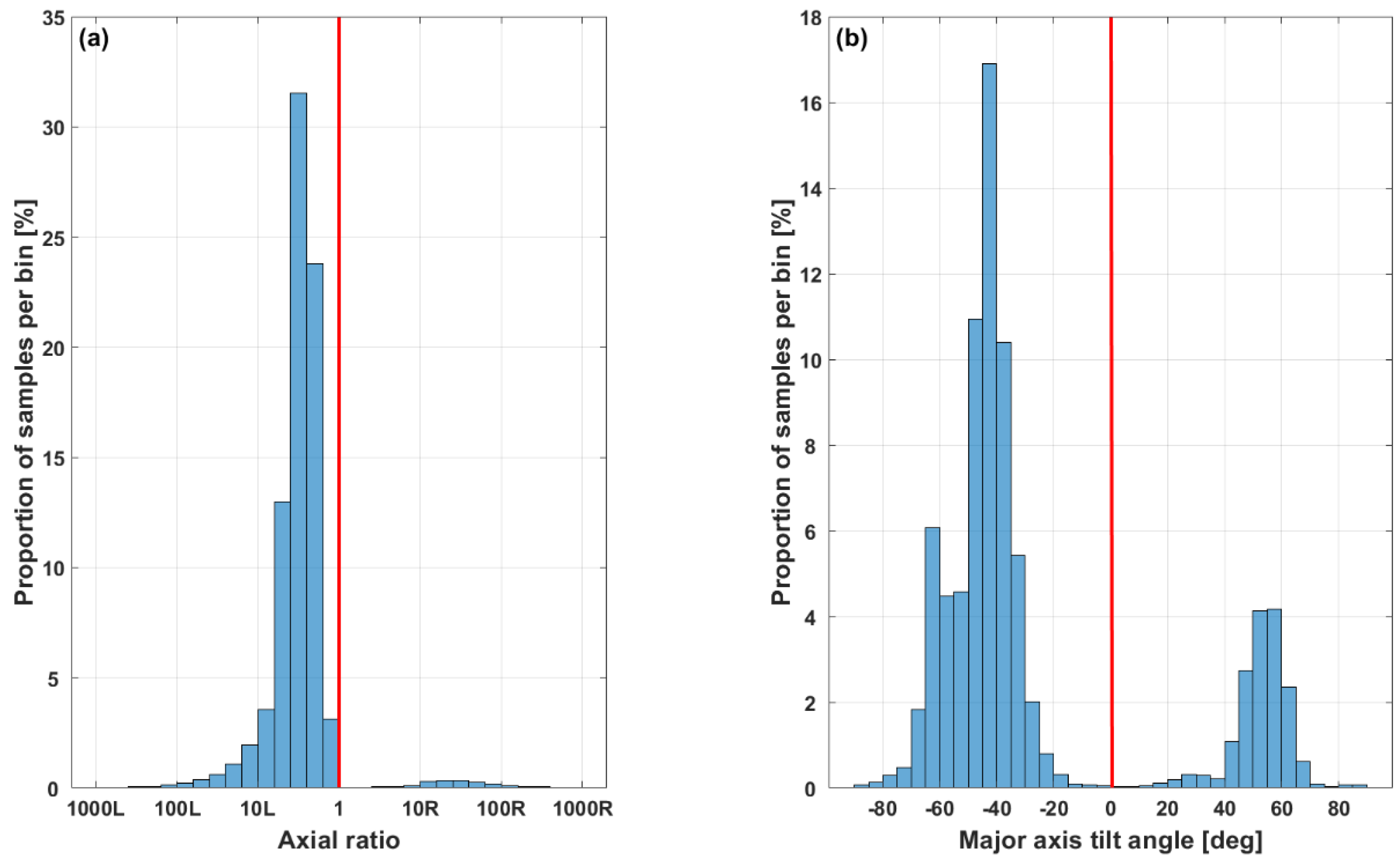
Figure 11 show the distribution of axial ratio and tilt angle measurements for each beacon in histogram form. In each figure, histogram (a) shows measured axial ratio on the horizontal axis on a logarithmic scale, with circular polarization marked by the red line in the center. Left-hand elliptical polarization is to the left of the red line and right-hand elliptical polarization is to the right of the red line. Similarly, histogram (b) shows measured tilt angle, with the red line marking 0° (horizontal) and with negative angles to the left, positive angles to the right. In each case, the vertical axis is the percentage of the total measurements in each bin.
Each individual sample represents a complete measurement of the properties of the polarization ellipse. The main sample rate used in the campaign was 6000 samples s−1, although some early measurements were made at 24,000 samples s−1. The selection of sample rate was a pragmatic decision based on a tradeoff between measurement cadence and received bandwidth, because it was necessary to capture a large enough bandwidth to allow the analysis of both components of a frequency shift keyed beacon signal, and also to be able to find nearby clear frequencies for background noise and calibration measurements. To ensure consistency in the data plotted on the histograms, measurements made at the higher cadence were normalized to 6000 samples s−1 in the analysis.
For the Faroe Islands beacon (
Figure 6), it can be seen that the polarization of the signal varied over a wide range during the 40 min analyzed, which was made up of regular extracts from a continuous sporadic-E reflection event which was 119 min long. According to this analysis there was no clearly preferred sense of rotation, with right-hand and left-hand elliptical polarization occurring roughly equally and, in each case, a calculated median magnitude of the axial ratio of about 3. Although tilt angle varied widely, there was a clear preference for angles around −50°.
In the case of Spain (
Figure 7), both senses of rotation were again observed, but with a clear preference for right-hand elliptical polarization and a calculated median axial ratio of just under +3. The tilt angle for the polarization ellipse varied widely, with a broad primary peak at about +55° and a secondary peak at about −80°.
The results from Sardinia (Italy) (
Figure 8) are similar to those from Spain, again with a clear preference for right-hand elliptical polarization and with a calculated median axial ratio of just under +3. The variation in tilt angle was also similar to Spain, but in this case the primary peak was around +50°.
The distribution of polarization states of the signal from Veneto (Italy) (
Figure 9) is much more similar to that observed from the Faroe Islands, with a near-symmetrical axial ratio distribution. The sense of rotation reversed many times during the recording, although in this case there was a slight preference for left-hand elliptical polarization over right-hand. The calculated median of the left-hand elliptical measurements (only) is at an axial ratio of about −4, remembering that axial ratio is defined as negative for a left-hand sense of rotation (
Section 2.3). Tilt angles again varied widely, albeit with a broad peak in the distribution centered at about +15°.
Finally, the polarization histograms for the beacons in Slovenia (
Figure 10), and Hungary (
Figure 11) look quite different from the other beacons. Each shows a very well-defined sense of rotation and a narrow peak in axial ratio. But the Slovenian signals exhibit distinct left-hand elliptical polarization, with a calculated median axial ratio of −3.1, whereas the Hungarian signals exhibit very clear right-hand elliptical polarization with a calculated median axial ratio of +3.6. Tilt angles also show a comparatively narrow range of variation, with Slovenia exhibiting a strong peak around −45° and Hungary showing a strong peak in the opposite quadrant, at about +45°, see
Section 3.2.
It can be seen from
Figure 6,
Figure 7,
Figure 8,
Figure 9,
Figure 10 and
Figure 11 that, across all the data, polarization states approaching linear—that is, with large axial ratio values—are comparatively rare. Signals from all the beacons, for the overwhelming majority of the time, are clearly elliptically polarized.
3.2. Case Study—Slovenia and Hungary Beacons
The second part of the study was a more detailed review of the data for the Slovenia and Hungary beacons, beyond the summaries in
Figure 10 and
Figure 11. As has been seen, the analysis for each beacon shows strongly defined elliptical polarization, but the sense of rotation and predominant tilt angle behaviours are consistently opposite from each other.
Firstly, we will consider a pair of individual recordings made only ten minutes apart on 18 August 2018, during a long period of intense sporadic-E over western Europe. The development and movement of this particular event is described in one of our earlier articles, which uses crowdsourced amateur radio reception reports as indicators of the presence of intense sporadic-E [
42]. Note that magnetic north was within 2° of geographical north in this part of Europe in 2018.
Figure 12 shows amateur radio signal reports from across Europe for the 15-min period which includes the ‘case study’ polarization measurements. Superimposed on the map are the locations of the beacons, and the great circle paths from the beacons to the receiving site in the UK. The great circle midpoints are marked, as approximate indications of the sporadic-E reflection points. It can be seen from the map that the two great circle midpoints are over southern Germany, about 200 km apart, and that there is strong evidence for the presence of intense sporadic-E in that area, at that time [
43]. These two reflection events are close in time and in the approximate location of the reflection point, so it is possible that they were both produced by a single large Es cloud.
To illustrate the consistent difference in polarization for signals over these adjacent paths,
Supplementary Video S1 shows a one-minute quasi-real time replay of the measured, normalized, polarization ellipse for the Slovenia beacon on 18 August 2018, and
Video S2 likewise for the Hungary beacon, recorded less than ten minutes later.
Figure 13 shows a snapshot from each video.
By contrast, referring back to
Figure 6, the signals from the Faroe Islands on 8 August 2018 show polarization varying over a wide range of axial ratio and tilt angle states. This behaviour was repeated at shorter timescales as well, as is very clearly illustrated in
Supplementary Video S3. This video shows two-minute quasi-real time replay of the measured, normalized, polarization ellipse for the Faroes beacon on 8 August 2018. It can be seen that the axial ratio, tilt angle, and sense of rotation are all constantly changing, on a timescale of seconds.
Using a Poincaré sphere to show how the measured polarization of a typical signal varies,
Figure 14 shows the 18 August 2018 case study data for the Hungarian beacon (two minutes duration) plotted as described in
Section 2.3.
From
Figure 14, a number of observations can be made. Firstly, all of the data is plotted onto the surface of the sphere rather than inside it. This indicates that the signal is consistently fully polarized. Secondly, there is a clear ‘home’ state for the polarization, in this case in the lower left front quadrant of the sphere, corresponding to right-hand elliptical polarization with a tilt angle between 0° and +45°. Deviations from the home state are present but there is a tendency to revert towards the home state. Thirdly, the deviations away from the home state can be seen to take smooth paths on the surface of the sphere rather than jagged, irregular paths, indicating a relatively smooth evolution of polarization. Gaps in the tracks indicate that some measurements have been rejected in post-processing because of low signal to noise ratio (see
Section 2.1).
Figure 15 (Slovenia) and
Figure 16 (Hungary) each show a set of representative Poincaré spheres to illustrate the general pattern of polarization behaviour over a number of days, with one sample sphere for each day that the beacon in question was observed.
It can be seen from
Figure 15 and
Figure 16 that the polarization states are broadly consistent across the full set of measurements of signals from each of Slovenia and Hungary. Both beacons show full polarization, with no indication of depolarization. It can be seen that there is, in each case, a relatively localized home state, although the range of deviations from it varies. The home state appears at various axial ratios and (particularly) a range of tilt angles on different days, but nonetheless the preferred sense of rotation is consistent for each beacon.
The tilt angle for the Hungary beacon is variable but is consistently between 0° and +90°, corresponding to the top right-hand quadrant of
Figure 4. The one outlier from a consistent pattern is the tilt angle for the Slovenia beacon, for which, although three of the spheres show negative tilt angles corresponding to the top left-hand quadrant of
Figure 4, one sphere—
Figure 15a—indicates tilt angles corresponding to the top right-hand quadrant of
Figure 4.
4. Discussion
4.1. Mode of Reflection
‘Scattering’ and ‘specular reflection’ have frequently been mentioned in the literature, since the early days of research into sporadic-E, as possible reflection mechanisms [
23,
24,
25]. The term ‘scatter’ has been used in the literature to describe a mechanism for producing weak sporadic-E signals, with differentiation being made between scatter and ‘true’ reflection on the basis of measured transmission loss [
23,
25]. According to this model, Es scattering is caused by irregularities in electron density, within an Es cloud, which are significantly larger than the wavelength of the incident wave but significantly smaller than the extent of the wavefront.
Ionospheric scattering of VHF radio waves [
44] (pp. 470–476) is caused by small-scale irregularities in electron density, the effect of which is to scatter energy away from the wave direction. At small angles to the wavefront, which are the most relevant to the current discussion (‘forward scatter’), the polarization of the incident wave is largely preserved [
45]. At larger scatter angles, increasing amounts of depolarization occur because of the random location, movement, and orientation of the scattering centers. Overall, scatter effects cannot change a linearly polarized wave into an elliptically polarized wave. Scatter from inhomogeneities within the sporadic-E layer may well cause the propagation of weak signals under some conditions, but it will not explain the properties of the stronger signals propagated via intense sporadic-E as observed in this study.
Turning now to the possibility of ‘specular reflection’, it is obvious that the term in its normal sense, referring to mirror-like reflection at a hard surface, cannot apply physically. The ionosphere is a partially ionized plasma; it does not consist of a closely-spaced matrix of atoms, such as in a metal or a solid dielectric, but rather is made up of randomly and widely-spaced ions and electrons which are in constant motion within the neutral atmosphere. The question is, therefore, whether signals returned from sporadic-E layers have similar characteristics to waves reflected from a hard surface, not whether they are actually being reflected from such a surface.
In the ionosphere, the refractive index at radio frequencies is always less than 1 and it decreases as ionization density increases [
44], so total internal reflection must be considered the most appropriate model. It can be shown [
46] (pp. 96–101), that total internal reflection of an electromagnetic wave at a dielectric surface introduces a fixed phase difference between the two components of the reflected wave parallel to and perpendicular to the surface. However, at the grazing angles of incidence relevant to long-distance reflection of 50 MHz waves from sporadic-E clouds, such a phase difference will be very small (<3°) [
47] (pp. 49–50), and dependent only on the alignment of the wave direction with the reflecting surface.
Although the internally reflected wave would therefore be slightly elliptically polarized rather than purely linear, reflection from such a ‘mirror’ could neither produce the large values of axial ratio and tilt angle reported in
Section 3, nor the observed variation of polarization behaviour with the orientation of the path to the geomagnetic field.
A clear result of our measurement campaign is that, in every case, the signals received were elliptically polarized after reflection from the Es cloud. This is despite the fact that all the beacons were known to be transmitting with linear polarization. Received signals exhibited no evidence of depolarization, and there are indications that polarization behaviour varied systematically depending on the orientation of the wave normal to the geomagnetic field at the point of reflection. This is convincing evidence that the mechanism for radio wave reflection was principally magnetoionic double refraction, rather than either scattering ‘or specular reflection’.
Even though the underlying physics must be the same, the physical differences between midlatitude Es layers and the normal ionospheric E layer are dramatic: Es layers are comparatively very thin, very intense, and very patchy, with a sharp ionization density gradient. These physical differences could plausibly lead to qualitatively different behaviour, but our research indicates that it is indeed the same reflection mechanism that is operating for sporadic-E, albeit very rapidly and over a very short distance within the Es cloud.
4.2. Detailed Polarization Behaviour
All the observed polarization features are consistent with magnetoionic double refraction within a variable-density sporadic-E layer, but a complete model would need to be able to explain more detailed polarization behaviour as well.
It can be seen from
Section 3.1 that, in most orientations to the magnetic field, all the key properties of the polarization ellipse—sense of rotation, axial ratio, and tilt angle—are highly variable. However as described in
Section 3.2, in the special case of the two paths which are closest to perpendicular to the geomagnetic field at the reflection point, much more stable elliptical polarization was observed over multiple sporadic-E reflection events, with consistently opposite polarization properties for the two paths.
To determine whether or not the ray path is perpendicular to the magnetic field vector requires the application of ray tracing and three-dimensional spherical geometry. Initial raytrace modelling (outside the scope of this article) using the PHaRLAP radio propagation toolbox [
48,
49] indicates that, for the paths from Hungary and Slovenia to the UK, the angle between the wave normal and the magnetic field vector does indeed pass through exactly 90° during the reflection process. The same modelling also indicates that the wave normal on the paths from the other four beacons is not perpendicular to the magnetic field vector at any point.
In general, it can also be shown that, as wave frequency increases, the two characteristic waves more closely approach circular polarization [
44] (p. 410). Specifically, the initial raytrace modelling shows that, in the cases of the Hungary and Slovenia to UK paths at 50 MHz, the downward characteristic waves will be very close to pure circular polarization. If this is the case, then if only one characteristic mode were present [
29] the downward wave would also have almost circular polarization, not clearly elliptical as the study results show. Therefore, the implication of the observed elliptical polarization is that both O and X are present in the signals monitored for this study.
On the assumption that the characteristic waves are indeed circularly polarized, it can be shown that the ellipse tilt angle of the combined polarization that emerges from the ionosphere will depend only on the phase difference between O and X. The characteristic wave phase difference can, in turn, be shown to depend on the ionization gradient within the sporadic-E layer. Therefore, the magnetoionic model can, in principle, explain the variability of axial tilt as the ionization density gradient changes.
The axial ratio and sense of rotation of the combined wave, however, will depend on the amplitude relationship between the O and X waves, in which case the experimental results (see, for example,
Figure 6) imply that frequently the amplitude ratio is itself highly variable. Absorption cannot explain this variation: non-deviative absorption at 50 MHz is very low and the difference in attenuation between the two characteristic modes is negligible. Explanation of the observed polarization properties may, therefore, require consideration of other factors, see
Section 4.3.
4.3. Application to Understanding the Physical Properties of Sporadic-E Layers
Much of the potential scientific value of this work lies in understanding more about the physical nature of Es, not just the way that radio waves propagate through it. We can speculate, for instance, that the observed variability of the tilt angle and axial ratio could be due to the uneven nature of the ionization in the Es cloud, leading to reflection from different ‘blobs’ of ionization as the cloud moves. Other effects might also be important, though, such as the physical shape of the region of an Es cloud which is dense enough to reflect at 50 MHz.
The fact that the Slovenia and Hungary data show so much less variation than the other paths, but with differing senses of rotation from each other, could be due to non-linear effects close to the reflection point, such as coupling between the two characteristic modes. Such coupling may take place where the wave polarization changes very rapidly with distance, and/or where the wave normal is close to perpendicular to the magnetic field vector [
44] (p. 83), both of which apply to our Hungary and Slovenia observations.
Prior work on oblique propagation paths [
50,
51] attempted to use measured sporadic-E transmission loss, along with Es critical frequency at the reflection point, to deduce the distribution of electron density in sporadic-E layers. Necessarily, this work made a number of assumptions about the structure of Es, specifically that it is an extremely thin ionized layer. Our approach, using polarization data to tease out information about the characteristic waves based on a magnetoionic analysis, may offer a more convincing alternative.
A fully-developed magnetoionic model of the interaction of radio waves with Es clouds poses challenges because of the very rapid variation of ionization with height, and hence the required granularity of the model. To answer the outstanding questions will also require the model to be able to represent the shape of the Es cloud, which could produce focusing, and to represent non-linear effects such as mode coupling.
The next phase of this work will focus on the development of a raytracing model which is appropriate for sporadic-E, without which any attempt to answer more detailed questions such as the causes of the spread in the properties of the polarization ellipse can only be speculative. This will be the subject of a future article.
5. Conclusions
This article reports the results of a radio wave polarization measurement campaign in the summer of 2018, which gathered a large amount of data at a receiving station in the south of the UK using six European 50 MHz amateur radio beacon transmitters as signal sources. Great circle paths were selected to be at a range of distances and a range of orientations to the Earth’s magnetic field.
Signals reflected from intense midlatitude sporadic-E clouds were found to be overwhelmingly elliptically polarized, across multiple paths and across multiple Es reflection events, despite the fact that they were transmitted with nominally linear polarization. Indications were also observed of the systematic variation of this behaviour with the angle of the path to the geomagnetic field at the reflection point. We have shown that neither ‘scattering’ nor ‘specular reflection’ could produce the observed polarization behaviour.
The primary objective of this research to date has been to demonstrate the true nature of sporadic-E reflection at VHF, and our results give strong evidence that, for the examples studied, it was primarily magnetoionic double refraction. We also found a remarkable and consistent disparity in the polarization of the reflections over the two paths closest to perpendicular to the geomagnetic field, which has never before been reported in the literature.
This technique has the potential to give further insight into the nature and structure of sporadic-E clouds. The focus of the next phase of work will be to explore the mechanisms producing the observed polarization states in more detail, and to relate that behaviour to the physical characteristics of the sporadic-E layers.
Finally, considering the temporal and spatial properties of the sporadic E clouds on a larger scale, sporadic-E is very patchy, and investigations would benefit from a denser network of observations than is currently available. A systematic and comprehensive study could greatly enhance understanding of the formation and structure of sporadic-E, presenting another opportunity for further work.


