Article

Predicting the Environmental Change of Carbon Emission Patterns in South Asia: A Deep Learning Approach Using BiLSTM

1
College of Computer Science, Huanggang Normal University, Huanggang 438000, China
2
School of Geography, Nanjing Normal University, Nanjing 210046, China
3
Department of Computer Engineering, Balochistan University of Information Technology, Engineering, and Management Sciences (BUITEMS), Quetta 87300, Pakistan
4
Department of Software Engineering, Balochistan University of Information Technology, Engineering, and Management Sciences (BUITEMS), Quetta 87300, Pakistan
5
Department of Computer Science, Balochistan University of Information Technology, Engineering, and Management Sciences (BUITEMS), Quetta 87300, Pakistan
6
Department of Electronic Engineering, Balochistan University of Information Technology, Engineering, and Management Sciences (BUITEMS), Quetta 87300, Pakistan
7
School of Information and Communication Engineering, Hainan University, Haikou 570100, China
*
Authors to whom correspondence should be addressed.
Atmosphere 2022, 13(12), 2011; https://doi.org/10.3390/atmos13122011
Submission received: 1 November 2022 / Revised: 15 November 2022 / Accepted: 28 November 2022 / Published: 30 November 2022

Abstract

:
China’s economy has made significant strides in the past three decades. As a direct result of China’s “one belt, one road” (OBOR) initiative, the country’s rate of industrialization and urbanization is currently the fastest in the entire world. This rapid development is largely dependent on the enormous amounts of energy currently being consumed and forms the foundation of the world’s high levels of carbon emissions. It is generally agreed that the production of greenhouse gases, particularly carbon dioxide, is the primary contributor to the current state of climate change. In this paper, a CO2 emission prediction model based on Bi-LSTM is constructed. In order to conduct empirical tests on the model, this study uses data from South Asian countries and China from 2001 to 2020. China’s CO2 emissions from 2022 to 2030 were predicted along with those of other countries in order to study the combined effects of the scientific and technological progress, industrial structures, and energy structure factors affecting CO2 emissions. When compared with the LSTM and GRU methods, the Bi-LSTM model’s results produced lower MAE, MSE, and MAPE values, indicating that it performs better. According to the findings, carbon emissions represent a significant problem that will become much worse in the future due to China and India’s high emissions, particularly in the next 10 years, if the government does not implement policies that help reduce those emissions.

1. Introduction

Since entering the 21st century, the world economy has developed by leaps and bounds, and the total global GDP has increased a lot each year [1]. The melting of Arctic ice and snow has accelerated, and global warming has increased significantly since the industrial revolution, both of which have severe consequences for human life and development. Scientists have come to the same conclusion about global warming: the increase in greenhouse gases, such as carbon dioxide, is the leading cause of the rise in temperature over the past 50 years. Eventually, carbon dioxide emissions will need to go down to almost zero because it has a long half-life as a greenhouse gas [2]. Earth’s air contains less than about 0.03 percent carbon dioxide, and it has remained essentially constant over a long period. The rate at which organisms in natural environments, such as volcanoes and hot springs, release gases into the atmosphere is equal to the rate at which terrestrial plants and marine organisms take in and fix carbon from the atmosphere and water through photosynthesis [3]. The ever-changing condition of “growth and consumption” is not in equilibrium. Human, animal, and plant respiration account for about 80% of atmospheric carbon dioxide, while the remaining 20% comes from the combustion of fossil fuels. Water bodies, like oceans, lakes, rivers, and other groundwater and air precipitation, absorb and dissolve 75% of the carbon dioxide dispersed into the atmosphere [4]. Plant photosynthesis converts an additional 5% of carbon dioxide into organic matter that can be stored. Since the industrial revolution, the carbon trapped in the formations of millions of years has been released in a relatively short period. Since the initial carbon cycle has been disrupted, it is estimated that the accumulated carbon dioxide will take between 50 and 100 years to be consumed and fixed through natural means [5].
China is still in the growth stage of carbon dioxide emissions and has not yet achieved carbon peaking. Under the development model dominated by the market economy with Chinese characteristics, China’s development trajectory to achieve carbon peaking is bound to have its own uniqueness. Countries that have reached the peak have different degrees of similarity. Under the premise of grasping the similarity, the reference to the social and economic development model of countries that have achieved carbon peaking is conducive to further clarifying the dynamic evolution relationship between social and economic development and carbon dioxide emissions [6]. Therefore, it is beneficial to make a preliminary judgment on the state of carbon emissions under the review of the current situation of China’s social and economic development. However, there is still a lack of relevant references for the socioeconomic development under the existing carbon peaking model; this has not helped to further reveal the impact of socioeconomic evolution on the carbon peaking process.
One belt one road (OBOR) is an important economic growth point in China in the next few decades [7], and it is one of the largest economic development areas. OBOR officially started construction and was upgraded to a national development strategy. Together, these came to form the Belt and Road Initiative (BRI), still formally known in Chinese as “One Belt, One Road”, including 78 countries in the world [8]; therefore, the OBOR plays a vital role in China’s economic development. OBOR is a substantial energy strategy implementation base in China and an essential ecological protection barrier in China. Therefore, the development of the OBOR is also related to environmental issues [9]. When ensuring economic development, it is necessary to maintain the stable operation of the ecological environment. The problems of environmental and economic growth will become more and more serious. At this stage, the economic development of OBOR mainly relies on industry, and a large amount of energy is inevitably consumed in the process of industrial production [10]. This problem is challenging to solve fundamentally, and China’s current policies and regulations related to carbon emissions are not perfect. These reasons undoubtedly increase the pressure on carbon emissions for OBOR. At present, the proportion of carbon emissions of the OBOR initiative to the national carbon emissions has remained at a relatively high level, and according to the trend in recent years, it has been increasing year-on-year. It can be said that it is the region with the largest carbon emissions in the country. This paper aims to analyze the influencing factors of carbon emissions in the OBOR countries, especially in South Asia and make a scientific forecast of its development trend from 2020 to 2035. According to the forecast results, it can provide a reference for the implementation of energy-saving and emission-reduction measures in the OBOR-selected countries. The carbon reduction and carbon peak targets of international commitments have been successfully achieved.
The main contributions of this study are:
  • The importance of carbon emissions, along the OBOR initiative, is increasing with time; therefore, this study, through a comprehensive study of the existing literature, provides the significance of the OBOR initiative for carbon emissions;
  • This study takes the circular economy and sustainable development as theoretical guidance. It deconstructs the carbon emissions in Chinese OBOR according to economic development, energy intensity, energy structure, urbanization level, and other aspects. The impact of various factors on carbon emissions is analyzed, and the future carbon emissions trend is predicted, judging the peak situation and putting forward the corresponding policy suggestions for carbon emissions reduction;
  • This study not only enriches the research on carbon emissions at the current stage but also provides a reference for local carbon emission reduction and provides a theoretical basis for China to achieve carbon neutrality as soon as possible. This study highlights the impact on the South Asia region due to the OBOR initiative.
Due to the advantageous geographical location of the OBOR, its carbon emission reduction results are directly related to the realization of China’s carbon emission reduction, carbon peaking, and even carbon neutrality goals. Studying carbon emissions in the OBOR will help develop a low-carbon economy and drive the development of emerging industries.

2. Literature Review

Different methods and applications exist in the literature for measuring carbon emissions, and these have been used for forecasting the current trends of emissions. Zhu et al. [11] comprehensively selected the carbon emission factors of the building materials widely used in the construction and retainment of walls in combination with building carbon emission calculation standards, raw materials, and building structure application technical guidelines. They then used the carbon emission factor method to calculate the retaining soil carbon emissions from the wall. Wu et al. [12] established a carbon emission factor calculation model for electricity and fossil fuels under the framework of the carbon emission calculation system for construction projects to estimate the carbon emissions in the construction process. For green buildings, Zhang et al. [13] proposed a quantitative calculation model for carbon emissions in the operation phase of green residential buildings, which was established from three aspects: the energy consumption of the building equipment, the greening of residential areas, and water systems. It was sued to calculate the total carbon emissions and various subitem carbon emissions of different star-rated green residential buildings in the operation stage.
Wu et al. [14] used the industrial sector in the Inner Mongolia Autonomous Region as the research object to calculate the carbon dioxide emissions of a plant using the carbon emission factor method and studied the relationship between carbon dioxide emissions and power supply. Ma et al. [15] divided asphalt pavement construction into different stages, and then used the carbon emission factor method to calculate the carbon dioxide emissions of each step, and then added them to obtain the carbon emissions of asphalt pavement construction so as to further carry out the analysis. Kneese et al. [16] calculated combustion carbon emissions based on the material balance method. The influence of coal composition on carbon emission and desulfurization cost was analyzed. The actual measurement method refers to the use of relevant equipment to measure the data about the emission source on the spot and then summarize the carbon emissions from the relevant emission sources. The advantage of this method is that the accuracy of the results obtained is high, but the disadvantage is that it is easy to be interfered with by external factors during field measurement, so the data are relatively difficult to obtain, and the input cost is high. In reality, most of the objects to be measured are first sampled on site, and then the samples are sent to the relevant testing departments, and special testing equipment and technologies are used for calculation and analysis. Therefore, this method is susceptible to errors regarding sample collection, sample representativeness, etc. Due to the interference of these factors, some scholars use this method to measure carbon emissions. Liu et al. [17] established a system framework on the basis of cyberphysical system (CPS) technology to monitor carbon emissions on construction sites in real time and developed a real-time carbon emissions monitoring system from hardware and software systems. Professional equipment, such as wireless sensors and servers, monitors and analyzes carbon emissions on construction sites.
Studying the influencing factors of carbon emissions is the key to solving the problem of carbon emissions. By reviewing the relevant literature over the years, it was found that most scholars’ research on the influencing factors of carbon emissions mainly includes changes in industrial structure, population, the technological environment, and energy consumption. At present, there are two main research methods used to study the influencing factors of carbon emissions in China, namely LMDI decomposition [18] and the STIRPAT model [19]. In order to study the influencing factors of carbon emissions in the Yangtze River Economic Belt, Liu et al. [20] took the influencing factors of carbon emission efficiency on the Yangtze River Economic Belt as the influencing factors of its carbon emissions and divided the influencing factors into economy, environment, industrial structure, foreign businessmen investment, technological innovation, and energy consumption, as six categories, and then a spatial panel measurement model was established; it concluded that economic growth could improve carbon emission efficiency, while the other five factors cannot have a positive impact on carbon emission efficiency. There are many influencing factors in this research, and some scholars have studied the relationship between a few of the factors of carbon emissions. Gong et al. took the OBOR as a research object, mainly analyzing the relationship between carbon emissions and industrial structure and environmental regulation in this region, and established a model based on the sample data for different years. Based on the panel vector autoregressive model, they combined impulse response function and variance analysis; it was concluded that there is a long-term equilibrium relationship between carbon emissions, industrial structure, and environmental regulation in the OBOR, meaning the three interact and promote each other. However, the article does not have a clear study on the impact of these two factors on carbon emissions. In addition to the literature on those factors affecting overall carbon emissions in the OBOR, a considerable number of scholars have chosen the industry within the OBOR to study those factors affecting carbon emissions [21,22]. The carbon emission factors of tourism in the OBOR were studied by Ahmed et al. [23], and seven factors, including economy, environmental pollution, tourism economy, tourism industry structure, tourism population, tourism energy consumption, and tourism energy consumption, were selected to establish the panel model; it showed that factors, such as tourism economy, population, energy consumption, and consumption structure, have a positive effect on tourism carbon emissions, while the other factors play a negative role in hindering them. Hu et al. [24] used an LMDI model to deconstruct the carbon emissions of the OBOR according to the factors, such as economy, industry, and energy intensity and structure. The two factors of industrial structure have a positive promotion effect on carbon emissions, while the energy intensity and energy structure factors have a reverse, hindering effect. Jiang et al. [25] used various data from the OBOR to establish a weighted factor decomposition model and combined the decoupling model to analyze the relationship between carbon emission decoupling and economy, energy intensity, and energy structure. It was found that economic and structural factors hinder the decoupling of carbon emissions, while energy intensity promotes the decoupling of carbon emissions [26]. Jahangir et al. [27] took Shanghai as the research object and used the STIRPAT model to study the development trend in the past two decades and analyze the influencing factors of its carbon emissions.
By reviewing the past literature, it was found that the domestic models for carbon emission prediction mainly include the STIRPAT model, the EKC prediction model, the grey prediction model, and the neural network and other models. But since the emergence of time-series machine-learning models [28], most studies these days use CNN, LSTM, etc., for carbon emission prediction. On the topic of time series data, a few related works have been carried out using machine learning, deep learning, and statistical models. The research of Masini et al. [29] examines the recent developments in supervised ML and high-dimensional models by considering linear and nonlinear techniques for time-series forecasting and blending the components of the ensemble and hybrid models. The economic and financial fields are another area where time-series forecasting is used. The predictive efficacy of various univariate models, including AutoRegressive (AR) models, was investigated by Crespo Cuaresma et al. [30]. An RNN model with a dimension-reducing symbolic representation was proposed by Elsworth et al. [31], which overcame the limitations of other models in the initialization of random weights and addressed the problem of the sensitivity of hyperparameters in any time-series model. Additionally, the speed of their model does not compromise the accuracy of their forecasts. Further, Amarpuri et al. [32] aimed to predict the CO2 levels in the year 2020 to make the government of India understand the challenges, and Zuo et al. [33] gathered the CO2 emission data from the various provinces of China and proposed a model named LSTM-STRIPAT, an integrated the model to predict emissions in 2020. The forecasting model is a deep learning hybrid consisting of a convolution neural network and a long short-term memory network (CNN-LSTM).
The research of Kumar et al. [34] used data from Delhi and the National Capital Region (NCR), India, to make predictions about the air quality index. Machine learning models have been implemented, and their efficacy has been evaluated using MAE, MSE, RMSE, and MAPE metrics. In another study [35], the authors applied and compared eight machine-learning models to data from the prestigious time-series competition. Specifically, the multilayer perceptron and the Gaussian process regression models fared the best. Nyoni and Bonga [36] utilized the Box–Jenkins method. The paper claims that the Chinese government is increasingly worried about air pollution and energy consumption in the iron and steel industries for power and coal, which accounts for a significant portion of the United States’ direct CO2 emissions, as sources of energy for the iron and steel industries. Instead of using traditional econometric methods, the authors here employ a machine learning approach, specifically a recurrent neural network called long short-term memory (LSTM), for the analysis of the relationship dynamics. Finally, they were able to provide evidence of a causal link between the iron and steel industries and CO2 emissions, which could inform policy decisions at the national level.

3. Materials and Method

3.1. Study Area

This study takes the OBOR South Asian countries and China as the study area (Figure 1). South Asia includes Afghanistan, India, Pakistan, Bangladesh, Sri Lanka, Nepal, Bhutan, and the Maldives: total population density 362.3/km2 (938/sq mi), with an area of 5,134,641 km2 (1,982,496 sq mi) and a population of 1.94 billion (2020). However, some would place Afghanistan more firmly in either Western or Central Asia or even in the Middle East. The region became a British protectorate after the Second Anglo–Afghan War and remained so until 1919. Although Myanmar (formerly Burma) was part of the British Raj from 1886 to 1937, it is now generally considered a part of Southeast Asia due to its membership in the Association of Southeast Asian Nations (ASEAN). Despite having been ruled by the British Raj at different points in history, neither the Aden Colony nor British Somaliland, nor Singapore has ever been considered to be a part of South Asia. Aksai Chin, formerly a part of the British Indian princely state of Jammu and Kashmir, is now a part of the Chinese autonomous region of Xinjiang and was claimed by India and may also be included in this area.

3.2. BiLSTM (Bidirectional Long Short-Term Memory Neural Network) Prediction Model

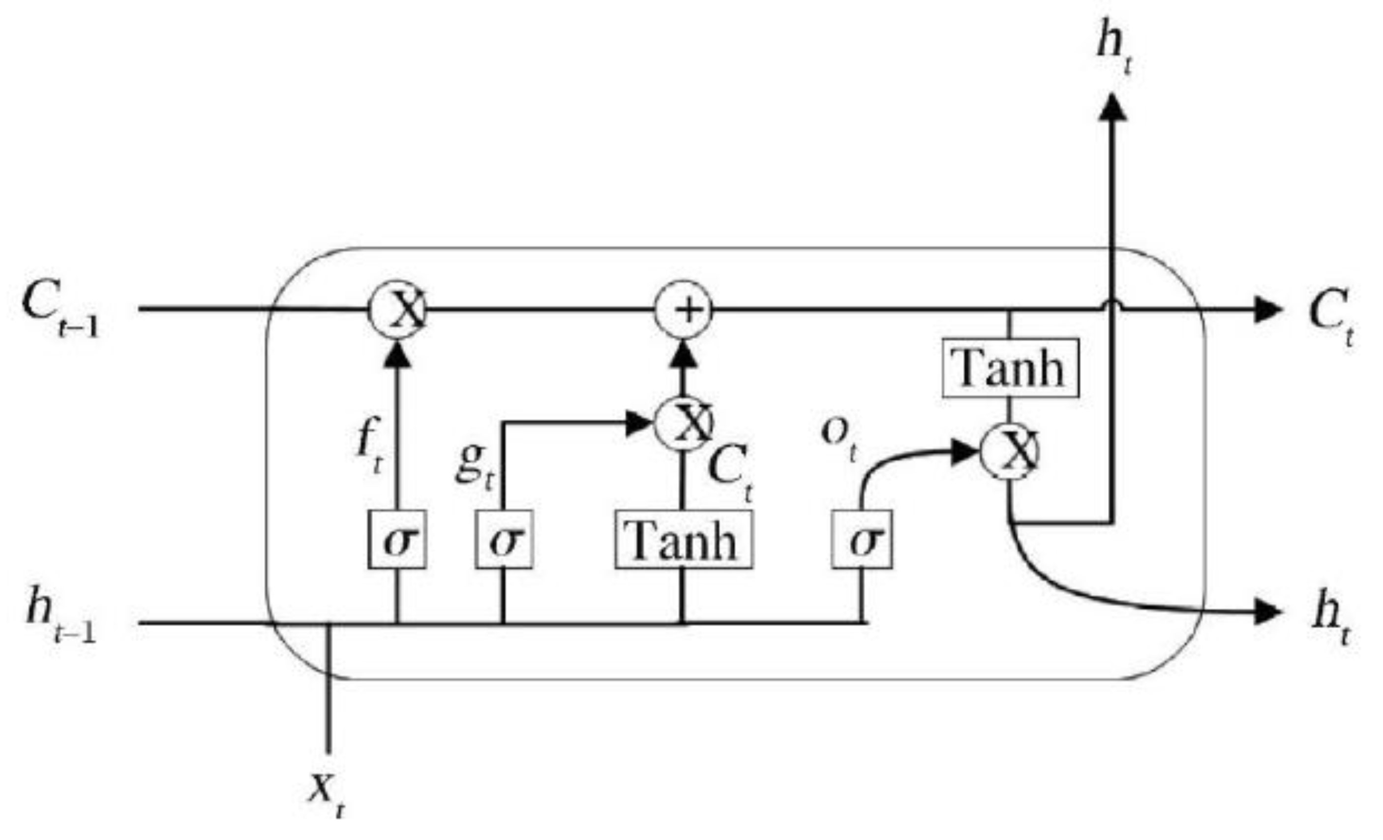
Recurrent neural networks (RNNs) can reflect the serial correlation characteristics of time-series data. Still, there are gradient disappearance or gradient explosion problems, so the mining of historical information for stock market data is limited. The LSTM neural network is a special RNN that has substantial advantages in dealing with the long-term dependencies of time-series data. As an extension of RNN, LSTM is clever in that it adds input gates, forgets gates, and output gates to obtain the changing self-circulation weights; when the model parameters are fixed, the integral scale at different times can be dynamically changed, effectively solving the existence of RNN and the vanishing gradient or exploding gradient problem. Figure 2 shows the structure of an LSTM neural network.
First of all, f t is the forget gate (forget gate); its role is to decide which information needs to be removed from the cell [37].
f t = σ b f + W f x t + U f h t 1
Among them, σ is the sigmoid activation function. x t is the current input vector, h t is the currently hidden layer vector, b f , W f , U f   are the bias, the input weight, and the loop weight of the forget gate, respectively.
Let g t be an external input gate between 0∼1 controlled by a sigmoid activation function:
g t = σ b g + W g x t + U g h t 1
Then, the updated cell state C t based on C t 1 is
C t = f t C t 1 + g t tanh b c + W c x t + U c h t 1
Finally, the information output controlled by the input gate (output gate) is h t = o t     tanh C t , where the output gate (controlled by the sigmoid activation function) is
o t = σ b o + W o x t + U o h t 1
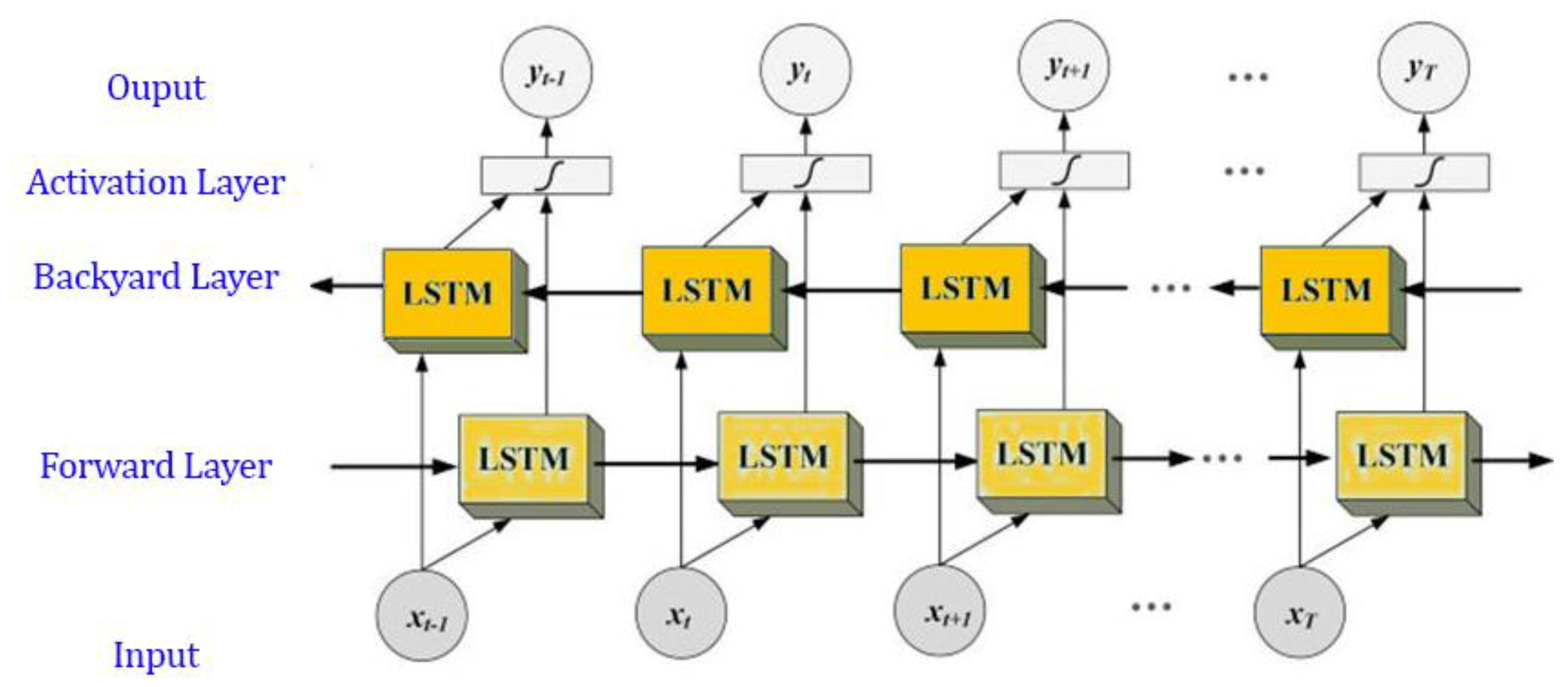
Since LSTM is unidirectional, it can only look at one side of a time-series relationship. The BiLSTM neural network comprises two LSTM neural networks, both of which receive the same input. Still, it is trained in opposite directions (forward and backward, respectively, as shown in Figure 3), with the LSTM neural network deciding on the final output in both directions.
The main formulas in BiLSTM are as follows:
h t = f w 1 X t + w 2 h t 1
h t = f w 3 X t + w 5 h t + 1
o t = g w 4 h t + w 6 h t
Among them, X t is the input at time t, w 1 , w 2 , w 3 , w 4 , w 5 , w 6 are the corresponding weight matrices, h t 1 is the output at the previous time, h t is the output at the forward layer at time t, h t + 1 is the output at the next time, h t   is the output at the reverse layer at time t, and o t is the output at time t.

3.3. Data

The data for this study were taken from the World Bank data [39] website from the years 1971 to 2020 for all the countries of South Asia, including Afghanistan, India, Pakistan, Bangladesh, Sri Lanka, Nepal, Bhutan, and the Maldives. This also used the data of China, which are focused on development OBOR in South Asia. In this study, we used the correlation coefficient (R), the mean squared error (MSE), the root mean squared error (RMSE), and the mean absolute error to assess the accuracy of the model (MAE). The fit between the predicted and actual values was measured using the correlation coefficient (R). MAE is proposed as the average difference between the actual and forecasted values, while MSE is the average difference between the actual and forecasted values, and RMSE is the square root of MSE. The outlier variance in the data is given more weight by RMSE than by MAE [40]. These metrics are calculated with the following formulas:
M S E = 1 n i = 1 n ( x i x ^ i ) 2  
  R M S E = 1 n i = 1 n ( x i x ^ i ) 2
  M A E = 1 n i = 1 n x i x ^ i
where x i and x ^ i are the actual and predicted values and n represents the number of samples.

4. Results and Discussion

4.1. Change in CO2 Emission Pattern in South Asia in Last 20 Years

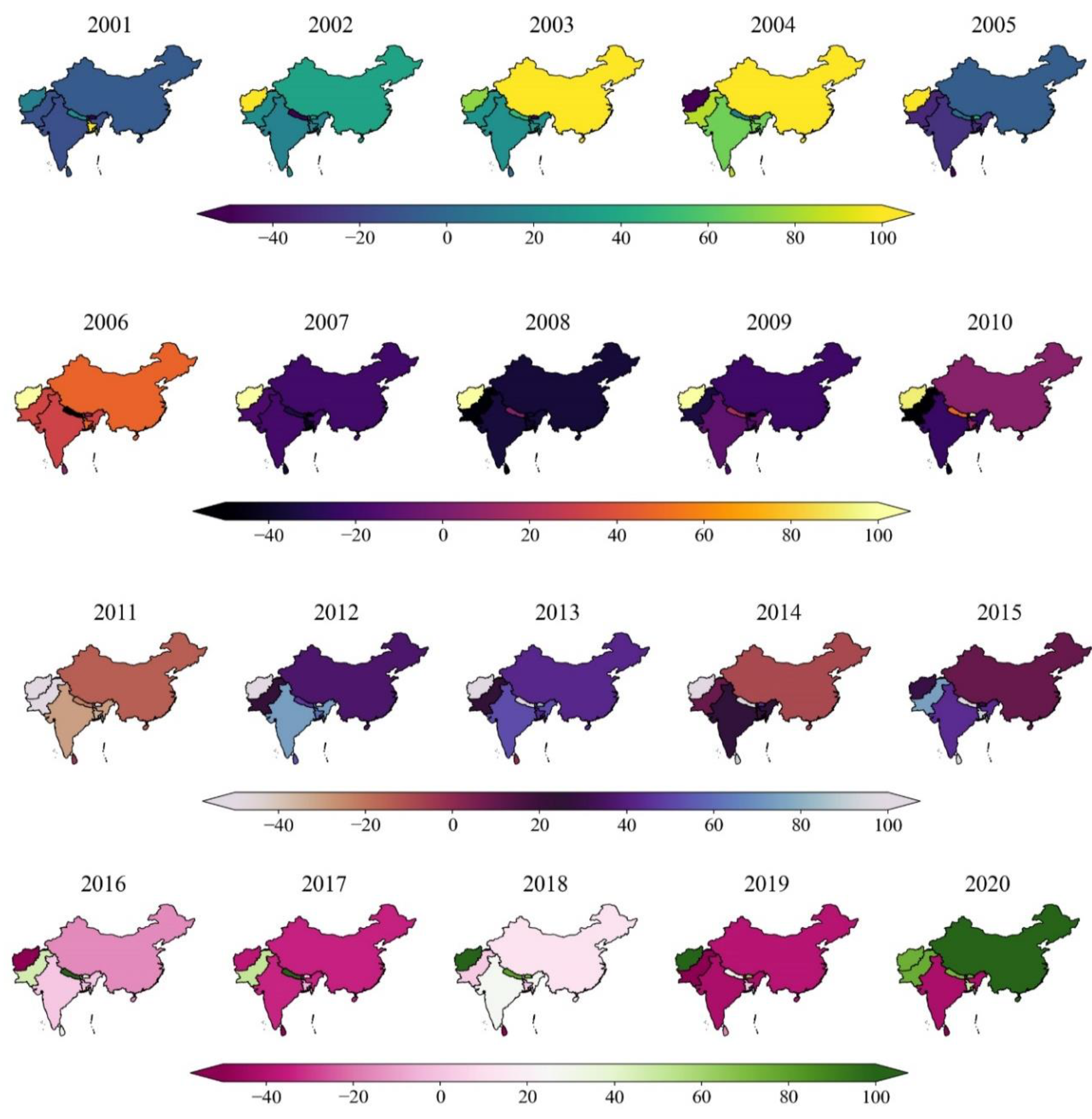
Figure 4 shows the significant increases in carbon emissions from 2001–2020. Afghanistan recorded a greater change in 2008 with an increase of 85% in carbon emissions, while in the last 20 years, the lowest decrease in carbon emissions occurred in 2004 at −25%. Similarly, a gradual increase in carbon emissions in Bangladesh and India was observed because of the yearly increase in GDP and industrialization, but that increase in emissions was steady and not too high. Before the Chinese program of the China-Pakistan Economic Corridor (CPEC), the emissions of carbon were lower in Pakistan because of the low increase in GDP, but as soon as the OBOR initiative emerged in 2013, the highest carbon emissions were observed in 2016 with a 22% rise with respect to last year. In the last few years, Srilanka has had many economic crises, with an observed decrease in carbon emissions, but after OBOR, it also has a similar pattern to Pakistan, with higher growth in 2014 at 21% due to the rise in GDP. Nepal’s economic development is increasing with respect to time, and this is causing an increase in carbon emissions; during the last five years, it has increased by 20% almost every year.
One of the most important aspects of trade policy is the way in which it affects economic expansion. The effects of trade openness on economic growth have been the subject of some theoretical models in previous research. Jallab et al. [41] looked into the connection between free trade and higher GDP growth in Morocco. The findings disproved the existence of a long-term causal relationship. Short-term, higher levels of trade activity led to higher GDP. However, Calderon et al. (2004) found no evidence of a growth effect due to openness in low-income countries, despite their conclusion that trade openness positively affects growth in high-income countries. With data from 126 countries, Freund and Bolaky [40] discovered that freer trade raises per capita income. They also found that economies with higher levels of flexibility saw a rise in living standards as a result of increased trade, while less flexible economies saw no such improvement. The time series analysis conducted by Sarkar et al. [42], however, found that trade openness had a negative effect on growth in India. The researchers measured openness through the ratio of trade to GDP. Furthermore, Chang et al. [43] believed that the positive relationship between growth and openness could be significantly strengthened through the implementation of supplementary policies.

4.2. Prediction of CO2 Emission Patterns in South Asia in the Last 20 Years

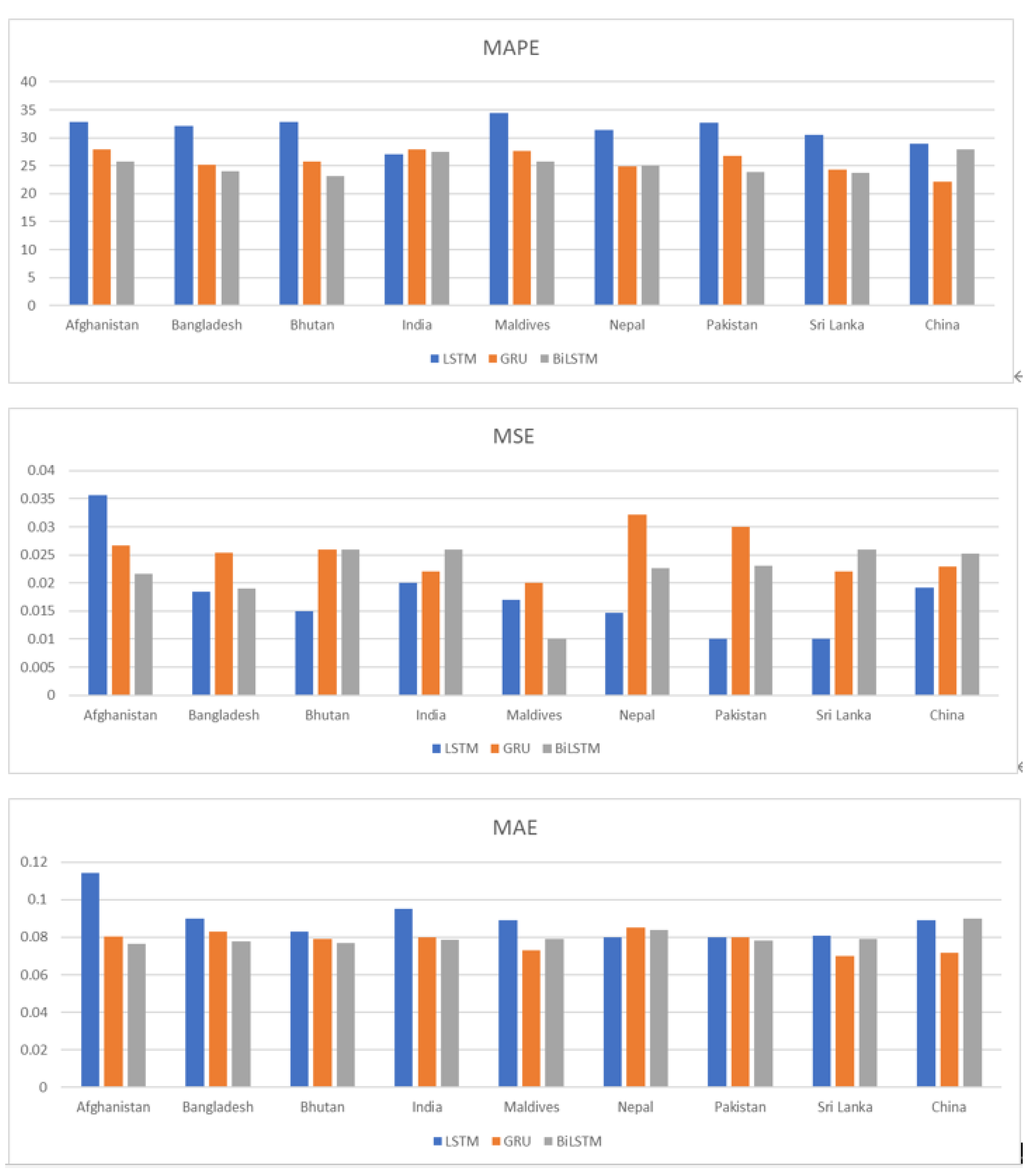
Three models (LSTM, GRU, and BiLSTM) were used to predict the pattern of carbon emissions from the training data covering 20 years, and the results are shown in Figure 5. When using the BiLSTM model, the MAPE values are as follows: Afghanistan: 25.77, Bangladesh: 24.07, Bhutan: 23.19, India: 27.52, Maldives: 25.77, Nepal: 24.99, Pakistan: 23.86, Sri Lanka: 23.7, and China: 27.97. When using GRU, the MAPE values are as follows: Afghanistan: 27.91, Bangladesh: 25.24, Bhutan: 25.7, India: 27.91, Maldives: 27.63, Nepal: 24.93, Pakistan: 26.78, Sri Lanka: 24.3, and China: 22.2. For LSTM, the MAPE values are as follows: Afghanistan: 32.86, Bangladesh: 32.18, Bhutan: 32.86, India: 27.01, Maldives: 34.41, Nepal: 31.39, Pakistan: 32.68, Sri Lanka: 30.59, and China: 28.94. The lowest MAPE values were observed using the BiLSTM model. Similarly, when using the BiLSTM method, the MSE values were as follows: Afghanistan: 0.02, Bangladesh: 0.02, Bhutan: 0.03, India: 0.03, Maldives: 0.01, Nepal: 0.02, Pakistan: 0.02, Sri Lanka: 0.03, and China: 0.03. For the GRU method, the MSE values are as follows: Afghanistan: 0.03, Bangladesh: 0.03, Bhutan: 0.03, India: 0.02, Maldives: 0.02, Nepal: 0.03, Pakistan: 0.03, Sri Lanka: 0.02, and China: 0.02. For LSTM method, the MSE values are as follows: Afghanistan: 0.04, Bangladesh: 0.02, Bhutan: 0.02, India: 0.02, Maldives: 0.02, Nepal: 0.01, Pakistan: 0.01, Sri Lanka: 0.01, and China: 0.02. The MAE values are also low for BiLSTM method: Afghanistan: 0.08, Bangladesh: 0.08, Bhutan: 0.08, India: 0.08, Maldives: 0.08, Nepal: 0.08, Pakistan: 0.08, Sri Lanka: 0.08, and China: 0.09.

4.3. Impact of CO2 Emission-Pattern Prediction in South Asia in the Next 10 Years

The annual growth rates in CO2 emissions for China and India are roughly the same (Figure 6). If the current prediction trend continues, then China will achieve 15 billion tons of carbon emissions (approximately), and India will be one of the biggest carbon emitters in the next 10 years, with 3.4 billion tons of carbon emissions. The emissions of growing countries were analyzed, and it was determined that economic development, as measured by per capita GDP, was the primary driver. This inference coincides with the findings of Wang et al. decomposition study [44]. However, as the Chinese economy entered new changes after 2012, their expansive economic growth was abandoned. China’s CO2 emission growth rate has also slowed considerably, and, on the macro scale, it has clearly decoupled from growth in the economy. This phenomenon likewise reflects the diminishing role of economic activity in driving emissions, which can be countered by the mitigating impact of emissions efficiency. One way in which energy intensity is diminished is through the enhancement of the industrial structure. Energy consumption can support moderate to rapid economic growth because the secondary sector’s share of GDP steadily declines as it becomes more energy intensive. The research on decoupling the economy and energy by Wang et al. [45] confirmed this inference. Cleaner energy is being used in China. Energy generation from renewable sources (such as wind, hydro, nuclear, and photovoltaic) has been growing in importance since 2012. The industrial structure and energy structure will be further optimized, and the inhibition effect on emissions is expected to improve if carbon peaking and carbon neutrality goals are followed.
An additional difficulty awaits Southeast Asia. Not only does it need to adjust to the effects of climate change, which has been brought on by decades of greenhouse gas emissions from developed economies like those of the United States and Europe and, more recently, from developing economies like China and India, but it also needs to change the development strategies that are increasingly contributing to global warming. OBOR brings new opportunities, but countries have to tackle climate change as well as economic growth [46]. Nation-wide efforts to reduce emissions and transition to cleaner energy sources are being undermined by the region’s increasing reliance on coal and oil. The effects of climate change are being amplified by rapid economic development and urbanization. People from the countryside are leaving to live in the warmer cities. Construction in the floodplains reduces flood protection because it blocks natural drainage routes, and as urban areas expand, the frequency and severity of flooding and storms will increase [47,48].
Similarly, India’s growing economy has resulted in increased carbon dioxide emissions. The decoupling state is in flux, so there is no discernible pattern of decoupling as of yet. Furthermore, population growth in India has historically been a more significant factor in CO2 emissions than in China. The analysis of consumption-based emissions in India also confirms that household consumption is the largest contributor to emissions in Indian states [49]. The increasing number of Indian citizens makes it imperative that the country adopt a low-carbon way of life. India’s energy and emission intensities have also been crucial in slowing the increase in CO2 emissions.
On the other hand, if current trends continue, India will need to increase its efforts to improve emission efficiency in order to counteract the pressure on CO2 emissions from future populations and economic growth. As another emerging developing nation, India cannot follow China’s example of excessive CO2 emissions. In light of the pressing need to limit global warming to 1.5 degrees Celsius, India must investigate options for economic development that minimize the country’s carbon footprint. As the government works to reduce its carbon footprint, it may be able to avoid carbon-intensive growth in developing regions by using sustainable planning and building practices rather than repeating the process of coupling and decoupling the economy and emissions.

5. Conclusions

If trends continue as predicted by the BiLSTM model, CO2 emissions will reach about 15 billion tons by the year 2030—roughly double the amount emitted today. Accurately projecting future emissions is useful for future governments as they craft policies to meet the specified reduction measures of the United Nations (UN), such as cutting emissions by 58% by that year. The policy suggestions for the future of environmental protection for government sectors and stakeholders are as follows:
  • One suggestion for government action is to increase levies on polluting industries;
  • A carbon tax, a cap-and-trade system, carbon offsets, a carbon cap, and standards for eco-friendly technologies;
  • Educate the public and help them become more aware of pollution problems;
  • Free bus policies and the promotion of electric vehicles have the potential to reduce the country’s overall fuel consumption and carbon footprint;
  • As a country on the rise in the renewable energy sector, India needs to reduce its reliance on coal in favor of cleaner energy sources like carbon-free hydrogen and sustainable biofuels;
  • Factories’ contributions to pollution can be reduced through the implementation of voluntary measures.
Carbon intensity predictions across the holdings in a portfolio can shed light on the underlying trends of the portfolio as a whole. It allows us to determine which predictions are the best and which are the worst. It is very instructive to compare the predicted changes in carbon intensity with the actual reported figures. It helps shareholders identify those companies that appear to be on a path toward steady progress in intensity reduction, as well as those that have diverged from the norm (positively or negatively).

Author Contributions

Conceptualization, A.W.; Data curation, M.A., M.A.B., S.M., A.W., A.H. and U.A.B.; Formal analysis, M.A., A.M.M. and U.A.B.; Funding acquisition, M.A., S.M.; Investigation, M.A., M.A.B., S.U.B., S.M., A.M.M., A.W., A.H. and U.A.B.; Methodology, M.A.B., S.U.B., A.W. and A.H.; Resources, S.U.B. All authors have read and agreed to the published version of the manuscript.

Funding

This study was funded by Huanggang Normal University, China, Selftype Project of 2021 (No. 30120210103) and 2022 (No. 2042021008).

Institutional Review Board Statement

Not applicable.

Informed Consent Statement

Not applicable.

Data Availability Statement

Not applicable.

Acknowledgments

Thanks to the reviewers and editors for their suggestions during the review process.

Conflicts of Interest

The authors declare no conflict of interest.

References

  1. Mansouri, K.; Alti, A.; Roose, P.; Laborie, S. Dynamic semantic-based green bio-inspired approach for optimizing energy and cloud services qualities. Trans. Emerg. Telecommun. Technol. 2018, 29, e3305. [Google Scholar] [CrossRef] [Green Version]
  2. Collins, W.J.; Bellouin, N.; Doutriaux-Boucher, M.; Gedney, N.; Halloran, P.; Hinton, T.; Hughes, J.; Jones, C.D.; Joshi, M.; Liddicoat, S.; et al. Development and evaluation of an Earth-System model—HadGEM2. Geosci. Model Dev. 2011, 4, 1051–1075. [Google Scholar] [CrossRef] [Green Version]
  3. Zhang, R.; Wang, Y.; Pang, Y.; Zhang, B.; Wei, Y.; Wang, M.; Zhu, R. A Deep Learning Micro-Scale Model to Estimate the CO2 Emissions from Light-Duty Diesel Trucks Based on Real-World Driving. Atmosphere 2022, 13, 1466. [Google Scholar] [CrossRef]
  4. Zhong, W.; Haigh, J.D. The greenhouse effect and carbon dioxide. Weather 2013, 68, 100–105. [Google Scholar] [CrossRef]
  5. Galvan, L.P.C.; Bhatti, U.A.; Campo, C.C.; Trujillo, R.A.S. The Nexus Between CO2 Emission, Economic Growth, Trade Openness: Evidences From Middle-Income Trap Countries. Front. Environ. Sci. 2022, 10, 938776. [Google Scholar] [CrossRef]
  6. Yu, K.M.K.; Curcic, I.; Gabriel, J.; Tsang, S.C.E. Recent advances in CO2 capture and utilization. ChemSusChem Chem. Sustain. Energy Mater. 2008, 1, 893–899. [Google Scholar] [CrossRef]
  7. Qayyum, M.; Yuyuan, Y.; Bhatti, U.A.; Shijie, L. Evaluation of the one belt and one road (OBOR) in economic development and suggestions analysis based on SWOT analysis with weighted AHP and entropy methods. Multimed. Tools Appl. 2022, 1–22. [Google Scholar] [CrossRef]
  8. Hasnain, A.; Sheng, Y.; Hashmi, M.Z.; Bhatti, U.A.; Hussain, A.; Hameed, M.; Marjan, S.; Bazai, S.U.; Hossain, M.A.; Sahabuddin, M.; et al. Time Series Analysis and Forecasting of Air Pollutants Based on Prophet Forecasting Model in Jiangsu Province, China. Front. Environ. Sci. 2022, 10, 945628. [Google Scholar] [CrossRef]
  9. Jiang, Q.; Ma, X.; Wang, Y. How does the one belt one road initiative affect the green economic growth? Energy Econ. 2021, 101, 105429. [Google Scholar] [CrossRef]
  10. Wang, Q.S.; Su, C.W.; Hua, Y.F.; Umar, M. Can fiscal decentralisation regulate the impact of industrial structure on energy efficiency? Econ. Res.-Ekon. Istraživanja 2021, 34, 1727–1751. [Google Scholar] [CrossRef]
  11. Zhu, Y.; Zhang, F.; Jia, S. Embodied energy and carbon emissions analysis of geosynthetic reinforced soil structures. J. Clean. Prod. 2022, 370, 133510. [Google Scholar] [CrossRef]
  12. Wu, Y.; Yang, Z.; Lin, B.; Liu, H.; Wang, R.; Zhou, B.; Hao, J. Energy consumption and CO2 emission impacts of vehicle electrification in three developed regions of China. Energy Policy 2012, 48, 537–550. [Google Scholar] [CrossRef]
  13. Zhang, Y.; Wang, J.; Hu, F.; Wang, Y. Comparison of evaluation standards for green building in China, Britain, United States. Renew. Sustain. Energy Rev. 2017, 68, 262–271. [Google Scholar] [CrossRef]
  14. Wu, R.; Zhang, J.; Bao, Y.; Lai, Q.; Tong, S.; Song, Y. Decomposing the influencing factors of industrial sector carbon dioxide emissions in Inner Mongolia based on the LMDI method. Sustainability 2016, 8, 661. [Google Scholar] [CrossRef] [Green Version]
  15. Ma, F.; Sha, A.; Lin, R.; Huang, Y.; Wang, C. Greenhouse gas emissions from asphalt pavement construction: A case study in China. Int. J. Environ. Res. Public Health 2016, 13, 351. [Google Scholar] [CrossRef]
  16. Kneese, A.V.; Ayres, R.U.; d′Arge, R.C. Economics and the Environment: A Materials Balance Approach; Routledge: London, UK, 2015. [Google Scholar]
  17. Liu, G.; Yang, H.; Fu, Y.; Mao, C.; Xu, P.; Hong, J.; Li, R. Cyber-physical system-based real-time monitoring and visualization of greenhouse gas emissions of prefabricated construction. J. Clean. Prod. 2020, 246, 119059. [Google Scholar] [CrossRef]
  18. Zhao, M.; Tan, L.; Zhang, W.; Ji, M.; Liu, Y.; Yu, L. Decomposing the influencing factors of industrial carbon emissions in Shanghai using the LMDI method. Energy 2010, 35, 2505–2510. [Google Scholar] [CrossRef]
  19. Wang, C.; Wang, F.; Zhang, X.; Yang, Y.; Su, Y.; Ye, Y.; Zhang, H. Examining the driving factors of energy related carbon emissions using the extended STIRPAT model based on IPAT identity in Xinjiang. Renew. Sustain. Energy Rev. 2017, 67, 51–61. [Google Scholar] [CrossRef]
  20. Liu, Q.; Hao, J. Regional Differences and Influencing Factors of Carbon Emission Efficiency in the Yangtze River Economic Belt. Sustainability 2022, 14, 4814. [Google Scholar] [CrossRef]
  21. Gong, M.; Zhen, S.; Liu, H. Research on the nonlinear dynamic relationship between FDI and CO2 emissions in the “One Belt, One Road” countries. Environ. Sci. Pollut. Res. 2021, 28, 27942–27953. [Google Scholar] [CrossRef]
  22. Fahim, A.; Tan, Q.; Bhatti, U.A.; Nawaz, S.A.; Kaleri, A.H. Urban Diversity Impact on Plant Species Due to Environmental Conditions. Pol. J. Environ. Stud. 2022, 31, 1617–1623. [Google Scholar] [CrossRef]
  23. Dong, B.; Xu, Y.; Fan, X. How to achieve a win-win situation between economic growth and carbon emission reduction: Empirical evidence from the perspective of industrial structure upgrading. Environ. Sci. Pollut. Res. 2020, 27, 43829–43844. [Google Scholar] [CrossRef] [PubMed]
  24. Ahmad, F.; Draz, M.U.; Su, L.; Ozturk, I.; Rauf, A. Tourism and environmental pollution: Evidence from the one belt one road provinces of Western China. Sustainability 2018, 10, 3520. [Google Scholar] [CrossRef] [Green Version]
  25. Hu, M.; Li, R.; You, W.; Liu, Y.; Lee, C.C. Spatiotemporal evolution of decoupling and driving forces of CO2 emissions on economic growth along the Belt and Road. J. Clean. Prod. 2020, 277, 123272. [Google Scholar] [CrossRef]
  26. Jiang, L.; Zhou, H.; He, S.; Cui, Y.; Wang, J. Identifying the driving factors of NO2 pollution of One Belt One Road countries: Satellite observation technique and dynamic spatial panel data analysis. Environ. Sci. Pollut. Res. 2021, 28, 20393–20407. [Google Scholar] [CrossRef]
  27. Jahanger, A.; Usman, M.; Balsalobre-Lorente, D. Autocracy, democracy, globalization, and environmental pollution in developing world: Fresh evidence from STIRPAT model. J. Public Aff. 2021, 22, e2753. [Google Scholar] [CrossRef]
  28. Bhatti, U.A.; Huang, M.; Wu, D.; Zhang, Y.; Mehmood, A.; Han, H. Recommendation system using feature extraction and pattern recognition in clinical care systems. Enterp. Inf. Syst. 2019, 13, 329–351. [Google Scholar] [CrossRef]
  29. Masini, R.P.; Medeiros, M.C.; Mendes, E.F. Machine learning advances for time series forecasting. J. Econ. Surv. 2021. [CrossRef]
  30. Crespo Cuaresma, J.; Hlouskova, J.; Kossmeier, S.; Obersteiner, M. Forecasting electricity spot-prices using linear univariate timeseries models. Appl. Energy 2004, 77, 87–106. [Google Scholar] [CrossRef]
  31. Elsworth, S.; Güttel, S. Time series forecasting using lSTM networks: A symbolic approach. arXiv 2020, arXiv:2003.05672. [Google Scholar]
  32. Amarpuri, L.; Yadav, N.; Kumar, G.; Agrawal, S. Prediction of CO2 emissions using deep learning hybrid approach: A case study in indian context. In Proceedings of the 2019 Twelfth International Conference on Contemporary Computing (IC3), Noida, India, 8–10 August 2019; pp. 1–6. [Google Scholar]
  33. Zuo, Z.; Guo, H.; Cheng, J. An LSTM-STRIPAT model analysis of China’s 2030 CO2 emissions peak. Carbon Manag. 2020, 11, 577–592. [Google Scholar] [CrossRef]
  34. Kumar, R.; Kumar, P.; Kumar, Y. Time series data prediction using IoT and machine learning technique. Procedia Comp. Sci. 2020, 167, 373–381. [Google Scholar] [CrossRef]
  35. Ahmed, N.K.; Atiya, A.F.; El Gayar, N.; El-Shishiny, H. An empirical comparison of machine learning models for time series forecasting. Econ. Rev. 2010, 29, 594–621. [Google Scholar] [CrossRef]
  36. Nyoni, T.; Bonga, W.G. Prediction of CO2 emissions in india using arima models. DRJ-J. Econ. Financ. 2019, 4, 1–10. [Google Scholar]
  37. Aamir, M.; Li, Z.; Bazai, S.; Wagan, R.A.; Bhatti, U.A.; Nizamani, M.M.; Akram, S. Spatiotemporal Change of Air-Quality Patterns in Hubei Province—A Pre-to Post-COVID-19 Analysis Using Path Analysis and Regression. Atmosphere 2021, 12, 1338. [Google Scholar] [CrossRef]
  38. Bhatti, U.A.; Wu, G.; Bazai, S.U.; Nawaz, S.A.; Baryalai, M.; Bhatti, M.A.; Hasnain, A.; Nizamani, M.M. A Pre- to Post-COVID-19 Change of Air Quality Patterns in Anhui Province Using Path Analysis and Regression. Pol. J. Environ. Stud. 2022, 31, 4029–4042. [Google Scholar] [CrossRef]
  39. World Bank Data. Available online: https://data.worldbank.org/indicator/EN.ATM.CO2E.PC (accessed on 30 September 2022).
  40. Bolaky, B.; Freund, C.L. Trade, Regulations, and Growth; World Bank Publications: Washington, DC, USA, 2004; Volume 3255. [Google Scholar]
  41. Jallab, M.S.; Abdelmalki, L.; Sandretto, R. The free trade agreement between the United States and Morocco: The importance of a gradual and assymetric agreement. J. Econ. Integr. 2007, 22, 852–887. [Google Scholar] [CrossRef]
  42. Sarkar, P. Trade openness and growth: Is there any link? J. Econ. Issues 2008, 42, 763–785. [Google Scholar] [CrossRef] [Green Version]
  43. Chang, C.C.; Mendy, M. Economic growth and openness in Africa: What is the empirical relationship? Appl. Econ. Lett. 2012, 19, 1903–1907. [Google Scholar] [CrossRef]
  44. Wang, C.; Chen, J.; Zou, J. Decomposition of energy-related CO2 emission in China: 1957–2000. Energy 2005, 30, 73–83. [Google Scholar] [CrossRef]
  45. Wang, Q.; Li, S.; Pisarenko, Z. Heterogeneous effects of energy efficiency, oil price, environmental pressure, R&D investment, and policy on renewable energy—Evidence from the G20 countries. Energy 2020, 209, 118322. [Google Scholar]
  46. Bhatti, U.A.; Nizamani, M.M.; Mengxing, H. Climate change threatens Pakistan’s snow leopards. Science 2022, 377, 585–586. [Google Scholar] [CrossRef]
  47. Bhatti, U.A.; Zeeshan, Z.; Nizamani, M.M.; Bazai, S.; Yu, Z.; Yuan, L. Assessing the change of ambient air quality patterns in Jiangsu Province of China pre-to post-COVID-19. Chemosphere 2022, 288, 132569. [Google Scholar] [CrossRef]
  48. Bhatti, U.A.; Yu, Z.; Chanussot, J.; Zeeshan, Z.; Yuan, L.; Luo, W.; Nawaz, S.; Bhatti, M.; Ain, Q.; Mehmood, A. Local Similarity-Based Spatial–Spectral Fusion Hyperspectral Image Classification With Deep CNN and Gabor Filtering. IEEE Trans. Geosci. Remote Sens. 2021, 60, 1–15. [Google Scholar] [CrossRef]
  49. Razzaq, A.; Wang, Y.; Chupradit, S.; Suksatan, W.; Shahzad, F. Asymmetric inter-linkages between green technology innovation and consumption-based carbon emissions in BRICS countries using quantile-on-quantile framework. Technol. Soc. 2021, 66, 101656. [Google Scholar] [CrossRef]
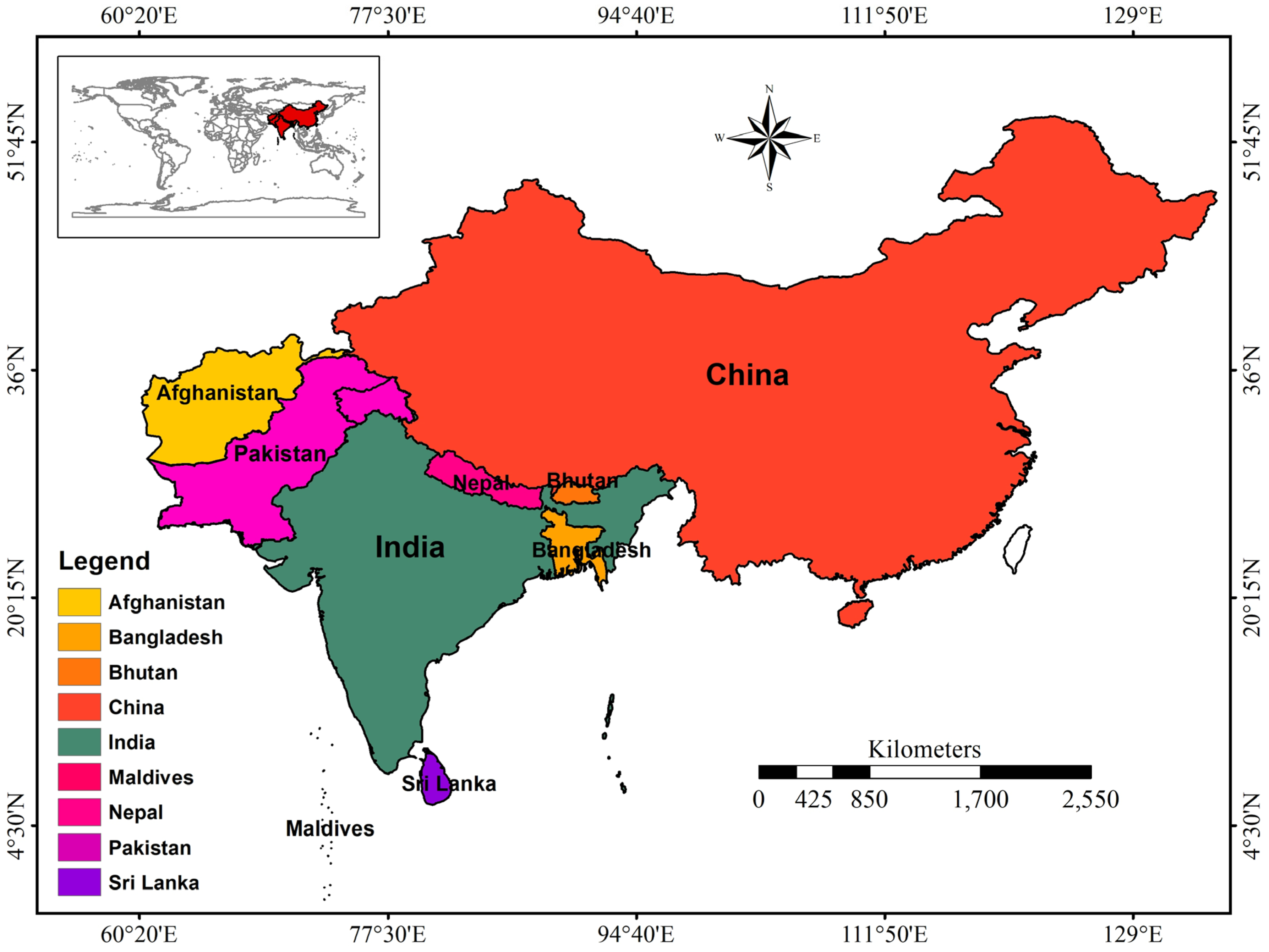
Figure 1. Study area of South Asia and China.
Atmosphere 13 02011 g001
Figure 2. LSTM implementation model [37].
Atmosphere 13 02011 g002
Figure 3. BiLSTM basic architecture [38].
Atmosphere 13 02011 g003
Figure 4. Change in CO2 emission patterns in South Asia in the last 20 years.
Atmosphere 13 02011 g004
Figure 5. The MAE, MSE, and MAPE of South Asian Countries and China.
Atmosphere 13 02011 g005
Figure 6. Carbon emissions in the last 20 years in China and South Asian countries.
Atmosphere 13 02011 g006
Publisher’s Note: MDPI stays neutral with regard to jurisdictional claims in published maps and institutional affiliations.