Article

Comparative Analysis of Secondary Organic Aerosol Formation during PM2.5 Pollution and Complex Pollution of PM2.5 and O3 in Chengdu, China

1
College of Architecture and Environment, Sichuan University, Chengdu 610065, China
2
Chengdu Academy of Environmental Sciences, Chengdu 610072, China
*
Author to whom correspondence should be addressed.
Atmosphere 2022, 13(11), 1834; https://doi.org/10.3390/atmos13111834
Submission received: 1 October 2022 / Accepted: 2 November 2022 / Published: 4 November 2022

Abstract

:
Nowadays, many cities in China are suffering from both fine particulate matter (PM2.5, particulate matter with an aerodynamic diameter smaller than 2.5 µm) and ozone (O3) pollution. Secondary organic aerosol (SOA) is an important component of PM2.5 and is closely related to the oxidation processes. To investigate the characteristics and formation pathways of SOA during different types of haze pollution episodes, carbonaceous components of PM2.5 and volatile organic compounds (VOCs) were monitored continuously in Chengdu in April 2019, when Chengdu experienced not only PM2.5 pollution (SPP) but also a complex pollution of PM2.5 and O3 (CoP). In the CoP episode, the concentrations of SOA increased by 51.2% as compared to SPP, and the SOA concentrations were positively correlated with PM2.5 mass concentrations. These suggest that SOA drove the increase in PM2.5 levels during the haze event to some extent. The preliminary VOC source analysis based on the feature ratio showed that vehicle emission and fuel volatilization sources were the main sources of VOCs at this urban site. In addition, coal emissions and biomass burning were also important contributors. High-carbon alkanes and aromatic hydrocarbons significantly contributed to the SOA formation. These results provide a preliminary understanding of SOA formation during different types of pollution episodes in Chengdu, which can help us to further understand air pollution in this typical region.

1. Introduction

Surface ozone (O3) and fine particulate matter (PM2.5, particulate matter with an aerodynamic diameter smaller than 2.5 µm) are major air pollutants in China [1,2]. Since the implementation of the Action Plan for Air pollution Prevention and Control (2013–2017) [3] and the Three-Year Action Plan to Win the Battle for Blue Sky (2018–2020) [4], PM2.5 concentration has decreased significantly across the nation [5]. However, current PM2.5 concentrations still regularly exceed the national air quality standard, and O3 pollution is becoming more and more severe [6]. Although high PM2.5 concentrations tend to occur in the cold seasons, and O3 pollution is more frequent in the warm seasons [1,7], there are days when PM2.5 and O3 pollution occur simultaneously, which is often referred to as the complex pollution of PM2.5 and O3 (CoP) [8,9,10].
Secondary organic aerosol (SOA) is a major component of PM2.5, which is generated through homogeneous and heterogeneous reactions of volatile organic compounds (VOCs) and intermediate/semi-VOCs as well as the aging of primary aerosols in the ambient atmosphere [11,12]. Meanwhile, the formation of O3 is closely related to VOCs and NOx. In other words, VOCs are one of the important precursors of secondary PM2.5 and O3 [13]. On the one hand, it can generate atmospheric oxidizing species such as O3 through photochemical reactions, thereby promoting the generation of secondary inorganic and organic components of PM2.5; on the other hand, it can also be directly converted into secondary organic components of PM2.5 [14,15]. Previous studies on SOA have typically involved the measurement of carbonaceous components [16,17] and SOA tracers [18,19] in PM as well as its gaseous precursors, VOCs [12,20].
The Sichuan Basin (SCB) is one of the most polluted areas in China [21]. Influenced by intense anthropogenic activities and frequent stagnant conditions as well as its complex basin topography, the SCB has suffered from severe PM2.5 and O3 pollution [7]. As the capital city of the SCB, Chengdu is a highly urbanized megacity, and its air pollution characteristics have attracted a lot of attention. In 2021, Chengdu was identified as one of the first cities in China to carry out the tracking study of “One City, One Policy” for the coordinated prevention and control of PM2.5 and O3 (https://www.mee.gov.cn/, accessed on 15 October 2022). However, as far as we know, previous air pollution studies on Chengdu mainly focused on single PM pollution [22,23,24,25] and single O3 pollution [26,27,28,29] as well as on the long-term characteristics of pollutants [30,31,32,33]. These studies also focused on the observation of individual PM2.5 components or individual VOC components. Only Song et al. [34] analyzed the formation mechanism of extreme haze events in Chengdu by simultaneously measuring PM2.5 components and VOCs. Furthermore, to our knowledge, few studies have characterized pollutants in CoP in Chengdu, which crucially limits our ability to coordinate the prevention and control of PM2.5 and O3 in this region.
In this study, we conducted a comprehensive online observation of the carbonaceous components of PM2.5 and VOCs in urban Chengdu from 1 April to 30 April 2019, during which a CoP episode occurred immediately after a PM2.5 pollution (SPP) episode. The purpose of this study was to perform a comparative analysis of these two types of pollution episodes, which mainly included investigating the amount of SOA generation and the characteristics of VOCs during the different episodes.

2. Materials and Methods
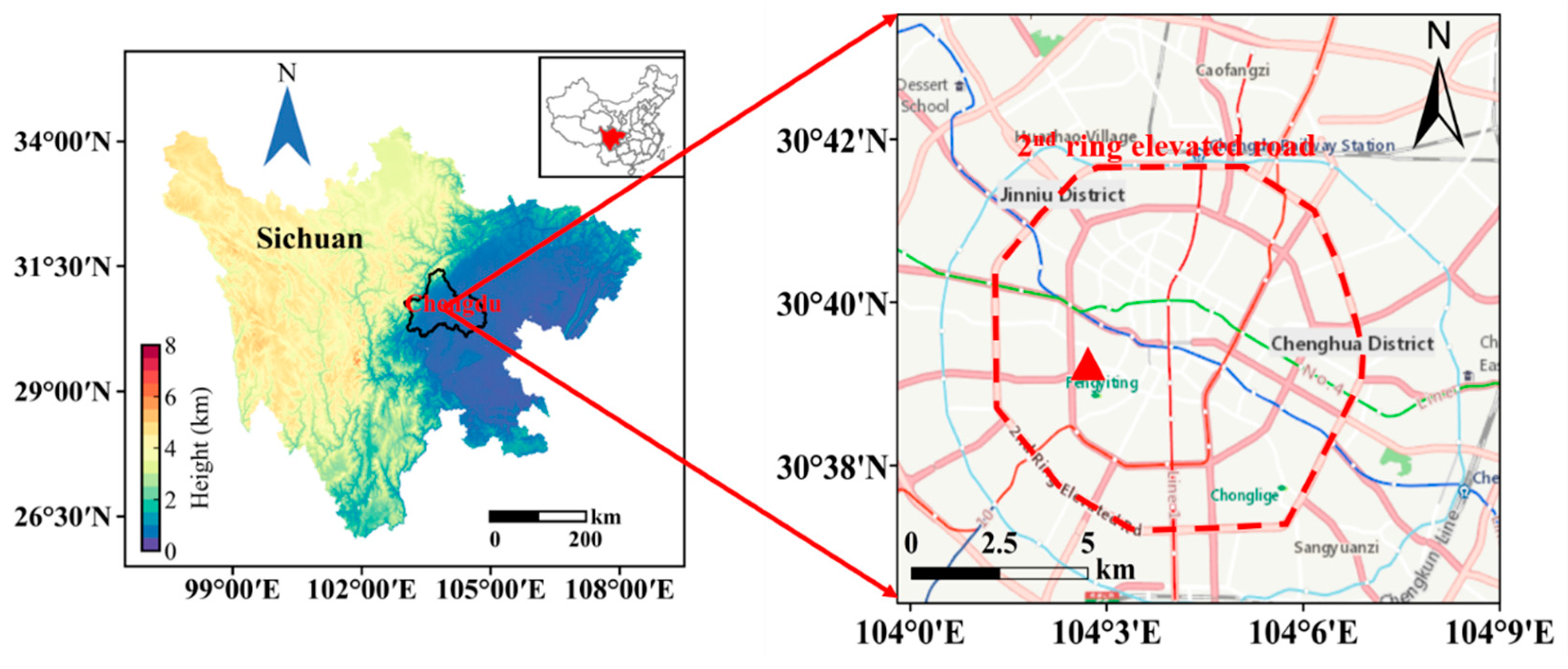
2.1. Sampling Site

The sampling site was located on the rooftop of the Chengdu Academy of Environmental Sciences in Qingyang District (30.65° N, 104.04° E, approximately 25 m above the ground). As shown in Figure 1, the site is located within the 2nd ring elevated road of Chengdu, surrounded by a mix of commercial and residential areas as well as dense traffic emissions, which make it a typical urban site in Chengdu [25,34].

2.2. Instruments

In this campaign, online monitoring instruments were used to obtain hourly resolution observations. All instrumental analyses were subject to regular laboratory quality control and quality assurance (QC/QA), including the strict enforcement of daily calibration and daily monitoring, which are detailed in a previous study [35]. PM2.5 concentrations were monitored by a tapered element oscillating microbalance instrument (TEOM 1405-F, Thermo Fisher, Waltham, MA, USA). Organic carbon (OC) and elemental carbon (EC) in PM2.5 were detected by a semi-continuous OC/EC analyzer (Type 4, Sunset Laboratories, Hicksville, NY, USA). Fifty-six VOC species were continuously monitored by a gas chromatograph (GC955-611/811, Synspec Corporation, Groningen, The Netherlands) with dual detectors, including a flame ionization detector (FID, for C2-C5 hydrocarbon measurements) and a dual photoionization detector (PID, for C6-C12 hydrocarbon measurements). Gaseous pollutants (NO2, NO, CO, and O3) were detected by a series of gas analyzers (17i/17i/48i/49i, Thermo Fisher, USA). In addition, a micro weather station instrument (WS600-UMB, Lufft, Fellbach, Germany) was used to measure the meteorological parameters, including temperature (T), relative humidity (RH), wind speed (WS), wind direction (WD), and precipitation (PP).

2.3. Data Analysis

2.3.1. Estimation of SOA in PM2.5

The minimum OC/EC ratio method has been widely used to estimate the concentration of SOC in particulate matters, which is calculated as shown below [36]:
POC = ( OC EC ) pri × EC
SOC = OC ( OC EC ) pri × EC
POA = 1.5 × SOC
SOA = 2.3 × SOC
where OC and EC are the measured concentrations of OC and EC in PM2.5, respectively; primary OC (POC) and SOC are the estimated primary and secondary organic carbon concentrations, respectively. The primary OA (POA) and SOA were calculated by multiplying the corresponding OC by the ratios of 1.5 and 2.3, respectively, which were obtained from online aerosol mass spectrometry observations conducted in the SCB [37]. From the above equation, it is clear that the critical step in estimating POC and SOC is the determination of an appropriate primary OC/EC ratio. In this study, the minimum R squared (MRS) method with a clear quantitative criterion was used to estimate the appropriate (OC/EC)pri value [16]. As shown in Figure S1, the actual (OC/EC)pri corresponding to the minimum R2 (SOC vs. EC) is 3.1.

2.3.2. Estimation of SOA Generation from VOCs

The atmospheric oxidation process of VOCs by OH radical, NO3 radical, and O3 was an important pathway for SOA generation [38]. To investigate the relationship between SOA and VOCs, we calculated the amount of SOA produced through the photochemical oxidation of VOCs based on the measured SOA yield in the smog chamber and the estimated VOC consumption [12,39]. The detailed calculation formula is as follows [12]:
SOA i = VOC i , consumed × Y i
where the VOCi,consumed is the consumption of ith VOC species; Yi is the SOA yield from the oxidation of the ith VOC species, determined by chamber studies. Previous studies have reported zero SOA yields for small alkanes and alkenes, low yields for higher (>C8) alkanes and cycloalkanes, and the highest SOA yields for aromatics [38]. In our study, the SOA yields for alkanes were taken from the study by Lim and Ziemann [40], and those for aromatics were recalculated by Wang et al. [12] based on a previous chamber study [39]. The vapor wall losses in the chamber studies were recognized to have been largely underestimated [12], and thus all the yields were also corrected by the vapor loss biases from Zhang et al. [41]. The SOA yields used in this study are tabulated in Table S1.
The photochemical consumption of VOCs can be calculated by Equation (7) below, with the assumption that the oxidation of OH radicals dominates the loss of VOCs in the ambient atmosphere.
VOC i , consumed = VOC i , t × ( exp ( k i [ OH ] Δ t ) 1 )
where VOCi,t and VOCi,consumed are the measured and consumed concentration of the ith VOC species, respectively; ki is the rate constant of the ith VOC species with OH radicals, cm3/molecule/s; [OH] and Δt are the OH radical concentrations and the determined photochemical age, respectively, and their product is the OH exposure.
The OH exposure is derived from the photochemical age, usually by selecting two VOC species of the same origin but with very different kOH values [42,43,44]. In this study, m, p-xylenes (X) and ethylbenzene (E) were selected to calculate the ambient OH exposure [43,45]. Hence, the OH exposure can be calculated as follows:
[ OH ] Δ t = 1 k X k E [ ln ( X E ) | t = 0 ln ( X E ) | t = t ]
in which kX and kE are the reaction rates of m, p-xylenes and ethylbenzene with OH radicals, respectively; ln(X/E)|t = 0 and ln(X/E)|t = t are the ratios of X/E for initial emission and observation, respectively.
As shown in Figure 2a, the concentrations of m, p-xylenes and ethylbenzene are highly correlated (r = 0.98). The initial emission ratios of m, p-xylenes and ethylbenzene were estimated by different methods, such as the 95th or 90th percentile method [12,20], the nighttime mean method [44], and the nighttime highest concentration method [45]. In our study, we tried different methods to estimate the initial emission ratio. As depicted in Figure 2b, the ratio estimated by the regression of nighttime concentrations is 3.3, while the ratio estimated by the 90th percentile method is 3.7; the latter seems to be more reasonable. Finally, the determined initial emission ratio of m, p-xylenes to ethylbenzene was 3.7 ppbv/ppbv.

3. Results and Discussion

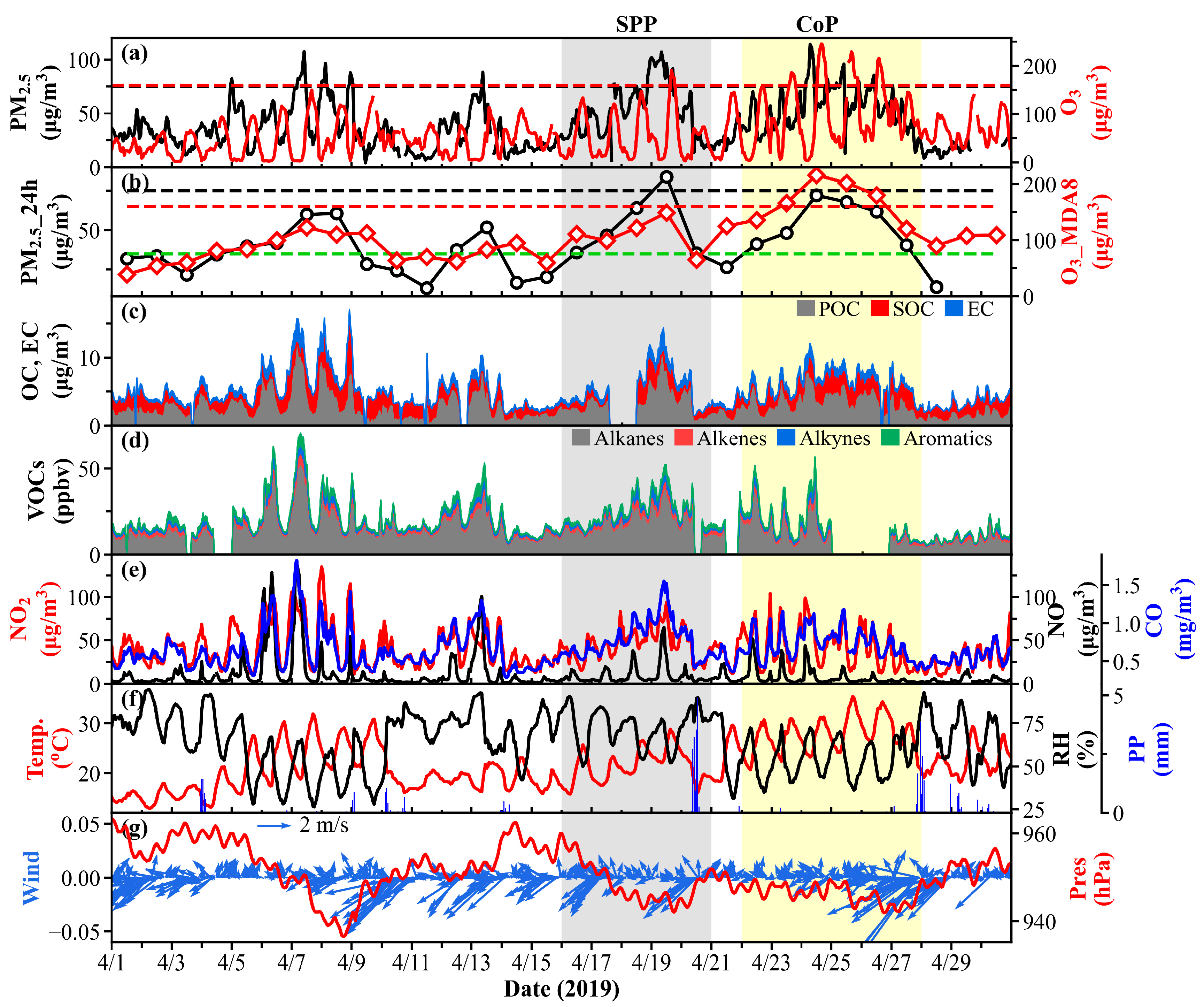
3.1. General Characteristics of Air Pollutants

Figure 3 shows the time series of PM2.5 and its carbonaceous components, O3, and VOCs from 1–30 April 2019. During the observation period, the highest hourly concentration of PM2.5 was 114.1 μg/m3 (at 7:00 on 24 April), while the hourly O3 reached its maximum (245.3 μg/m3) at 16:00 on 24 April (Figure 3a). According to China’s National Ambient Air Quality Standard (GB3095-2012), a haze pollution day was defined as a day with a daily average PM2.5 concentration exceeding 75 μg/m3 (the secondary standard threshold for daily average PM2.5 concentration), and an O3 pollution day was defined as a condition with a daily maximum 8 h average (MDA8) O3 concentration greater than 160 μg/m3 (the secondary standard threshold for MDA8 O3). A CoP day was defined as a day when PM2.5 pollution and O3 pollution were present at the same time. In order to cover the entire pollution process, days with PM2.5 greater than 35 ug/m3 during the development and dissipation phases of pollution were also considered. Based on the above definitions, there were two typical pollution episodes during our observation period: an SPP episode from 16–20 April 2019 and a CoP episode from 22–27 April 2019. As shown in Figure 3f, the end of these two pollution processes was significantly associated with the precipitation at noon on 20 April and at midnight on 28 April, respectively, indicating the beneficial effects of wet scavenging on spring air pollution.
Table 1 lists the mean values of each measured parameter for different pollution episodes. In general, PM2.5 concentrations were comparable during the two pollution episodes, with average concentrations of 53.2 ± 24.7 μg/m3 (SPP) and 55.3 ± 19.6 μg/m3 (CoP), respectively; however, O3 concentration in CoP (97.7 ± 63.9 μg/m3) was approximately twice as high as in SPP (54.3 ± 46.7 μg/m3), indicating that the atmospheric environment of the CoP was more oxidative. Meanwhile, the SOA concentration in CoP (6.5 ± 2.6 μg/m3) was also much higher than that in SPP (4.3 ± 3.2 μg/m3). More precisely, SOA generation in CoP increased by 51.2% as compared to SPP, highlighting the intense SOA generation in CoP. In addition, VOCs, an important precursor of SOA and O3, were at lower levels in CoP (34.4 ± 20.0 ppbv) than in SPP (44.8 ± 16.1 ppbv), which may be related to the stronger photochemical consumption during the CoP period. However, as for EC and CO, which are mainly derived from primary combustion processes [46], their concentrations during the two pollution episodes were very close, showing that emissions from combustion sources did not change much.
Pollutant concentrations are highly correlated with meteorological conditions. As listed in Table 1, the average wind speed during both pollutant episodes was low (~1 m/s), but the relative humidity and temperature varied considerably. During the CoP, higher temperature (27.7 ± 3.4 °C) and moderate relative humidity (54.6 ± 10.8%) were observed, which were favorable for the co-occurrence of O3 and PM2.5 pollution [8].

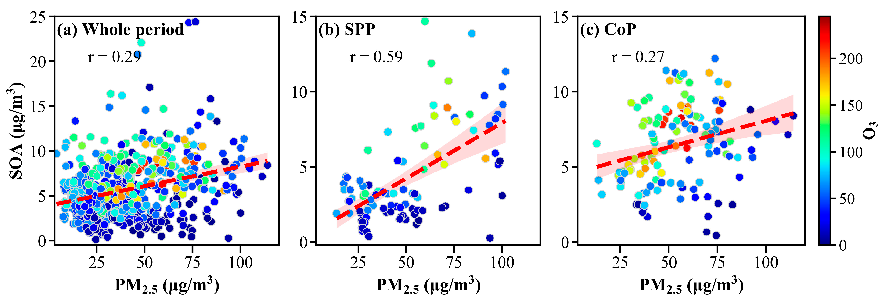
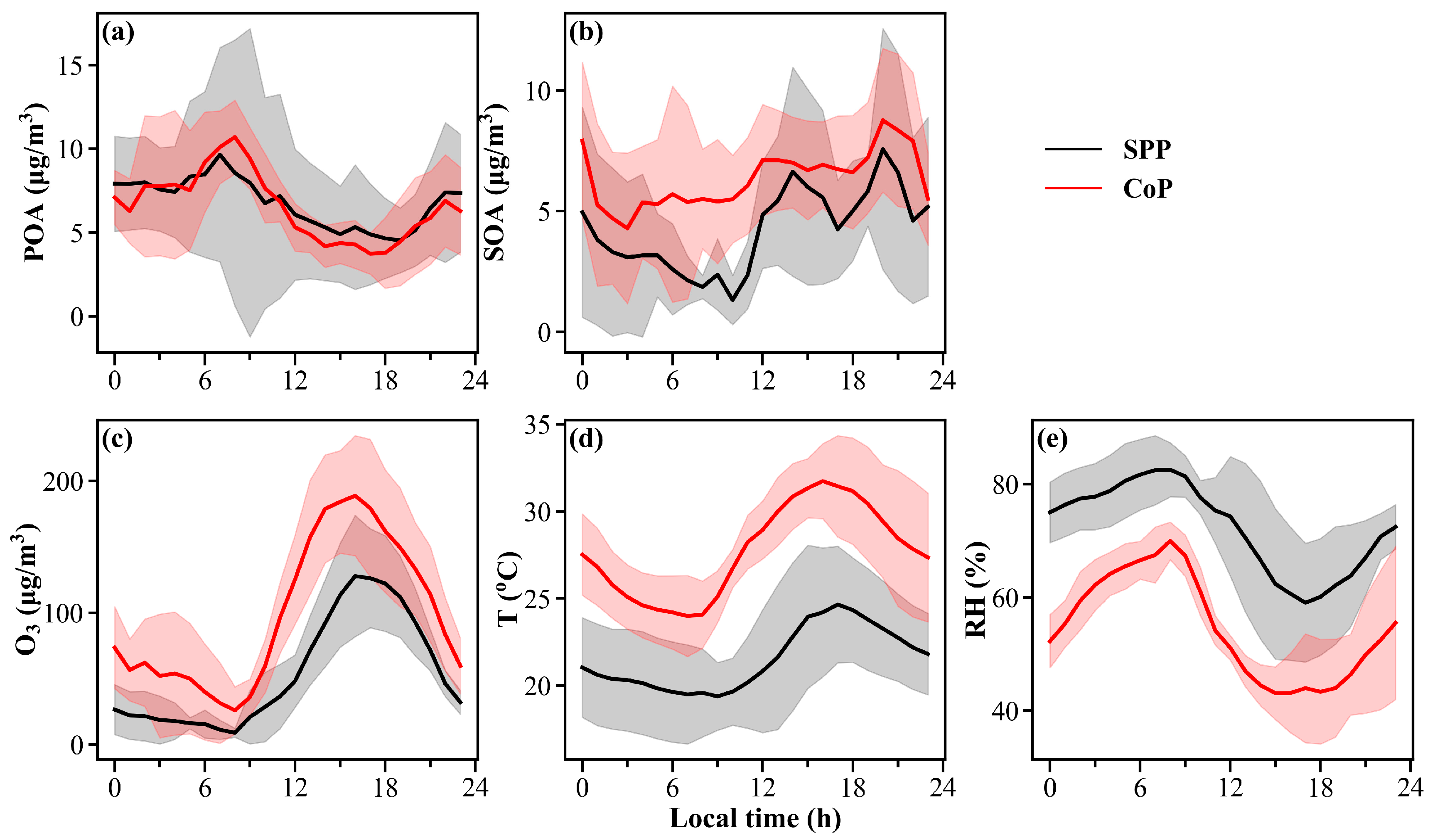
3.2. Characteristics of SOA in PM2.5

Figure 4 presents the scatter plots of SOA versus PM2.5 for different pollution episodes. It can be clearly seen that SOA concentration increased with PM2.5 (Figure 4a), suggesting that the generation of SOA promoted the increase of PM2.5; that is, the generation of SOA can promote the development of the spring haze pollution processes to some extent. Further analyses of the different episodes (Figure 4b,c) showed that the correlation between SOA and PM2.5 was stronger during SPP (r = 0.59) than CoP (r = 0.27). In addition, high SOA concentrations during SPP were concentrated at high PM2.5 levels (>50 ug/m3), and some high values of SOA were also observed at very low O3 concentrations, which may be attributed to the heterogeneous generation of SOA. However, during CoP, a high SOA concentration often occurred with high O3 concentration, highlighting the homogeneous generation of SOA.
To further understand the generation of SOA in different types of pollution episodes, the diurnal patterns of different carbonaceous components during the two pollution episodes were also investigated (Figure 5). During the different pollution episodes, the diurnal trend of POA was relatively consistent, peaking in the morning rush hours (6:00–9:00) and rising again in the evening rush hours (Figure 5a). However, the diurnal trend of SOA varied greatly among the different pollution processes. As shown in Figure 5b, the SOA in the SPP exhibited a clear daytime bimodal feature, where the first peak may have been influenced by the strong photochemical oxidation in the afternoon, while the second peak may be due to the evening peak commute, during which large amounts of precursors are emitted into the atmosphere and can be oxidized by residual oxidants. The diurnal trend of SOA was not significant during the CoP, with high SOA concentrations throughout the day. Meanwhile, the nocturnal SOA concentrations were higher in CoP than in SPP, which may have been affected by the high level of O3 and high temperatures at night (Figure 5c,d). In addition, SOA in CoP also exhibited a bimodal peak during the day, with the peak shifting forward at noon as compared to SPP, which may be related to the rapid increase in daytime temperature and light intensity during the CoP episode. Once the light intensity is sufficient, a strong atmospheric photochemistry occurs, which then promotes the photooxidative production of SOA [47].

3.3. Characteristics of Measured VOCs in Different Pollution Episodes

As listed in Table 1, the average mixing ratio of total VOCs (TVOCs) during the whole observation period was 36.2 ± 19.8 ppbv, which was higher than that in a previous study on Chengdu during the summer period (26.8 ± 14.9 ppbv) [32]. The levels of VOCs varied greatly among the different pollution episodes, with the mean mixing ratio of TVOCs in CoP (34.4 ± 20.0 ppbv) being only 76.8% of that in SPP (44.8 ± 16.1 ppbv). To further understand the characteristics of VOCs in different types of pollution episodes, this section will focus on comparing the composition, dominant species, and diurnal variation patterns as well as sources of VOCs during the two pollution episodes.

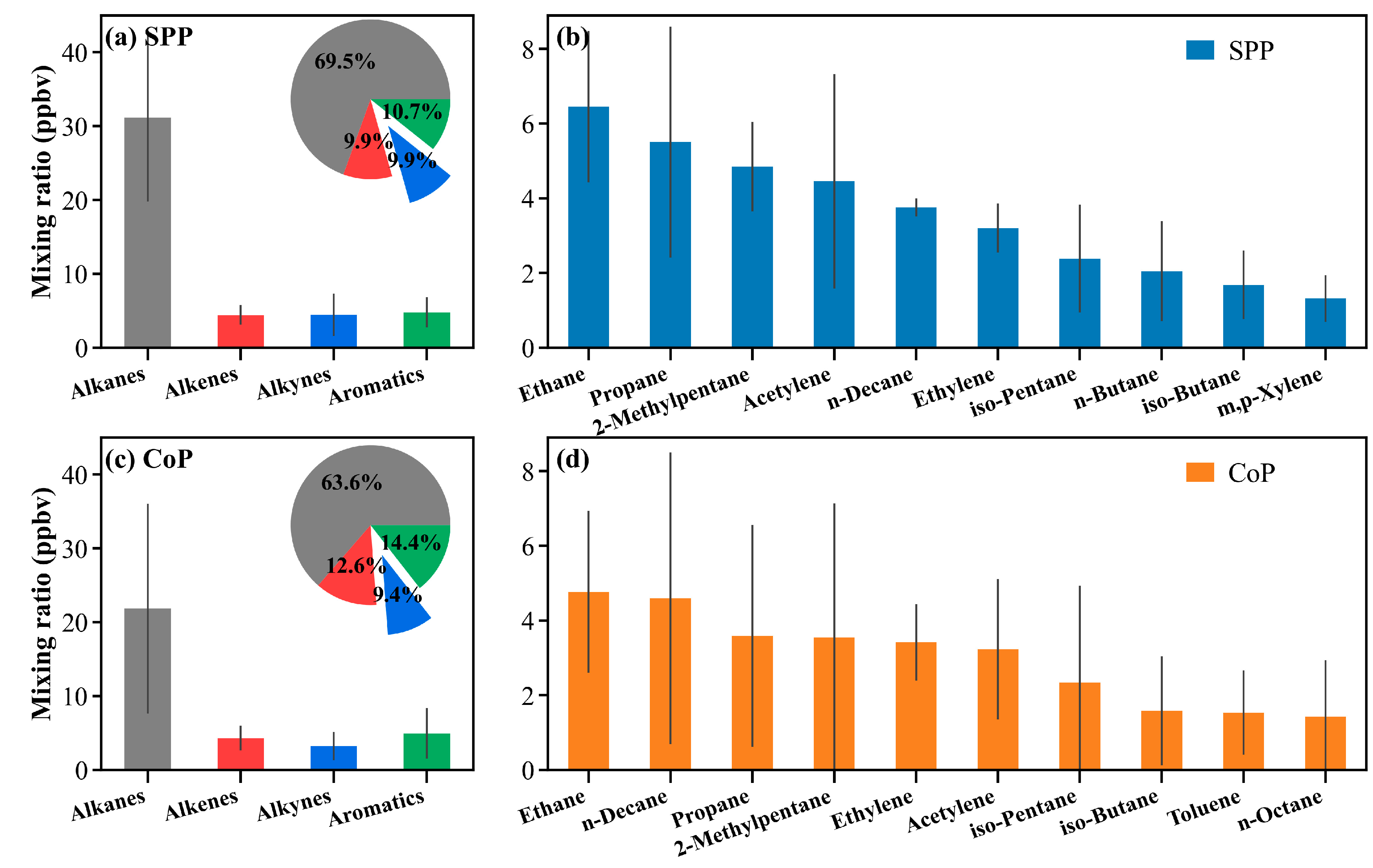
3.3.1. Measured VOCs Composition and Dominant Species

As shown in Figure 6a,c, the concentrations of different VOC groups in SPP and CoP varied considerably. Overall, the concentrations of TVOCs in CoP decreased as compared to those in SPP, with significant decreases in alkanes (−29.8%, from 31.1 ppbv to 21.8 ppbv) and alkynes (−27.5%, from 4.6 ppbv to 3.2 ppbv), while alkenes (from 4.4 ppbv to 4.3 ppbv) and aromatics (from 4.8 ppbv to 5.0 ppbv) remained almost unchanged. Although the proportion of different VOC groups varied slightly from episode to episode, the ranking was always alkanes >> aromatics > alkenes > alkynes. Figure 6b,d also displayed the top ten VOC species for both episodes. Ethane, n-decane, propane, 2-methylpentane, acetylene, ethylene, iso-pentane, and iso-butane were always detected in the top ten VOC species during SPP and CoP. Almost all VOC species in CoP were at lower levels than in SPP, which may be related to the stronger atmospheric oxidation in CoP.

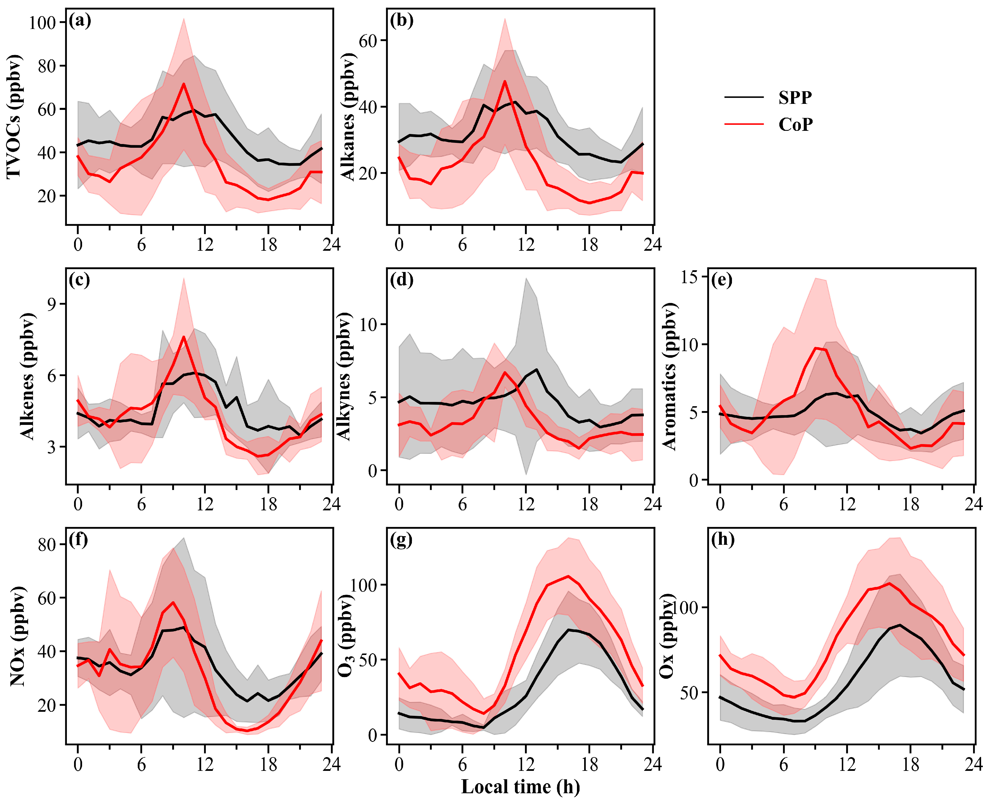
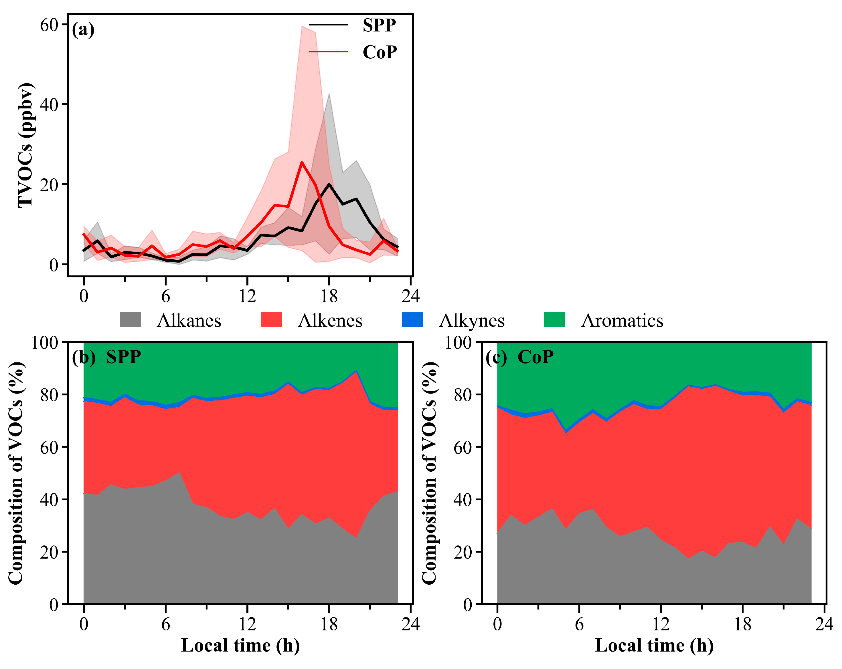
3.3.2. Diurnal Variations of VOC Groups

Figure 7 shows the diurnal variation of different VOCs groups, NOx (the sum of NO and NO2), O3, and Ox (the sum of O3 and NO2) for different pollution episodes. Overall, the diurnal variation of VOCs was consistent with that of NOx, but the opposite of O3. As shown in Figure 7a,c, both NOx and VOCs exhibited a peak at around 9:00 in the morning in these two episodes, which may have been influenced by strong emissions and weak atmospheric oxidation during the morning peak commute (Figure 7h). After the morning peak hour, VOCs in CoP continued to decrease until 18:00 and then increased again. Additionally, we observed that the peak of VOCs in SPP lasted for several hours (9:00–12:00), while the VOCs in CoP peaked only at around 9:00 and then decreased rapidly. This phenomenon may be influenced by the different diurnal patterns of light intensity in the different episodes. Furthermore, the levels of VOCs in CoP were lower than those in SPP at most moments, which may be due to the high levels of Ox in CoP. We also found that the peaks of O3 and Ox appeared earlier in CoP than in SPP, which were probably affected by the difference in diurnal temperature and the light variations in these two episodes (Figure 5e).

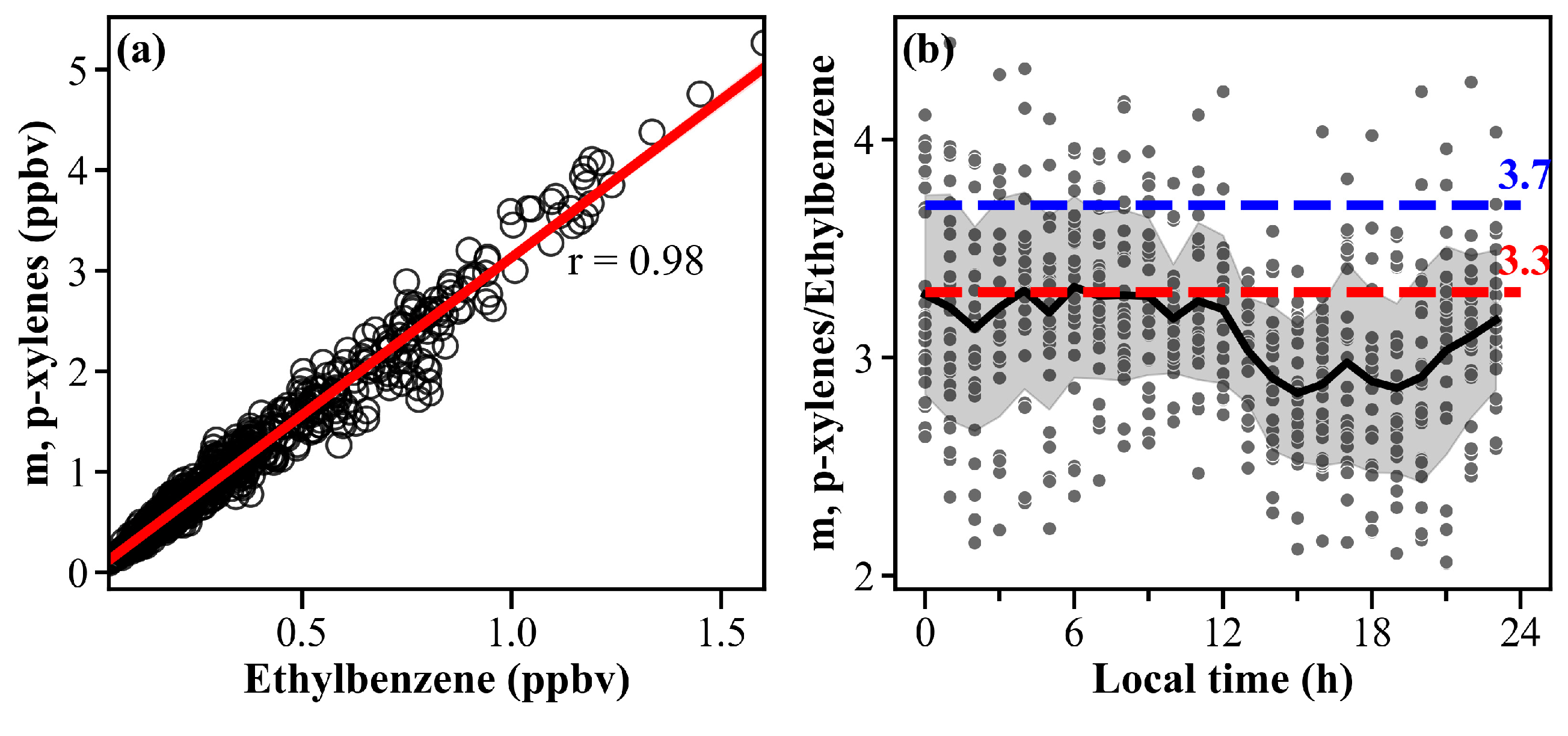
3.3.3. Source Analysis of VOCs Based on Species-Specific Ratios

The ratios of some specific species pairs can be applied to preliminarily determine the VOC emission sources [48,49,50]. For example, the toluene/benzene ratio is commonly used to identify the sources of traffic emissions, fuel combustion, and industrial and solvent usage [51,52]; the isopentane/n-pentane ratio can also be used to indicate different sources, including traffic emissions, coal combustion, liquid gasoline, and fuel volatilization [53]. The ratios of different species pairs from different sources have been summarized by Shi and co-authors [49].
The ratios of different species pairs in this study for different pollution episodes and other research works are listed in Table 2. The benzene/toluene ratios for SPP and CoP were 0.86 ± 1.57 and 0.75 ± 0.60, respectively, which were slightly higher than those for vehicle exhaust emissions (0.56–0.60), indicating the contribution of other high-rate sources (e.g., coal combustion emissions and biomass burning), especially for the SPP episode. The isopentane/n-pentane ratios varied significantly in SPP and CoP, with mean values of 2.65 ± 0.70 and 3.42 ± 1.12, respectively. The high isopentane/n-pentane ratios suggest that VOCs in urban Chengdu are mainly influenced by vehicle emission and fuel volatilization, with the isopentane/n-pentane ratios from these sources being 2.93 and 1.84–4.46, respectively. The extremely high isopentane/n-pentane ratio in CoP emphasizes the high contribution of volatile sources, including gasoline and fuel volatilization, which may be related to the high temperature that promotes oil and gas evaporation during this period.

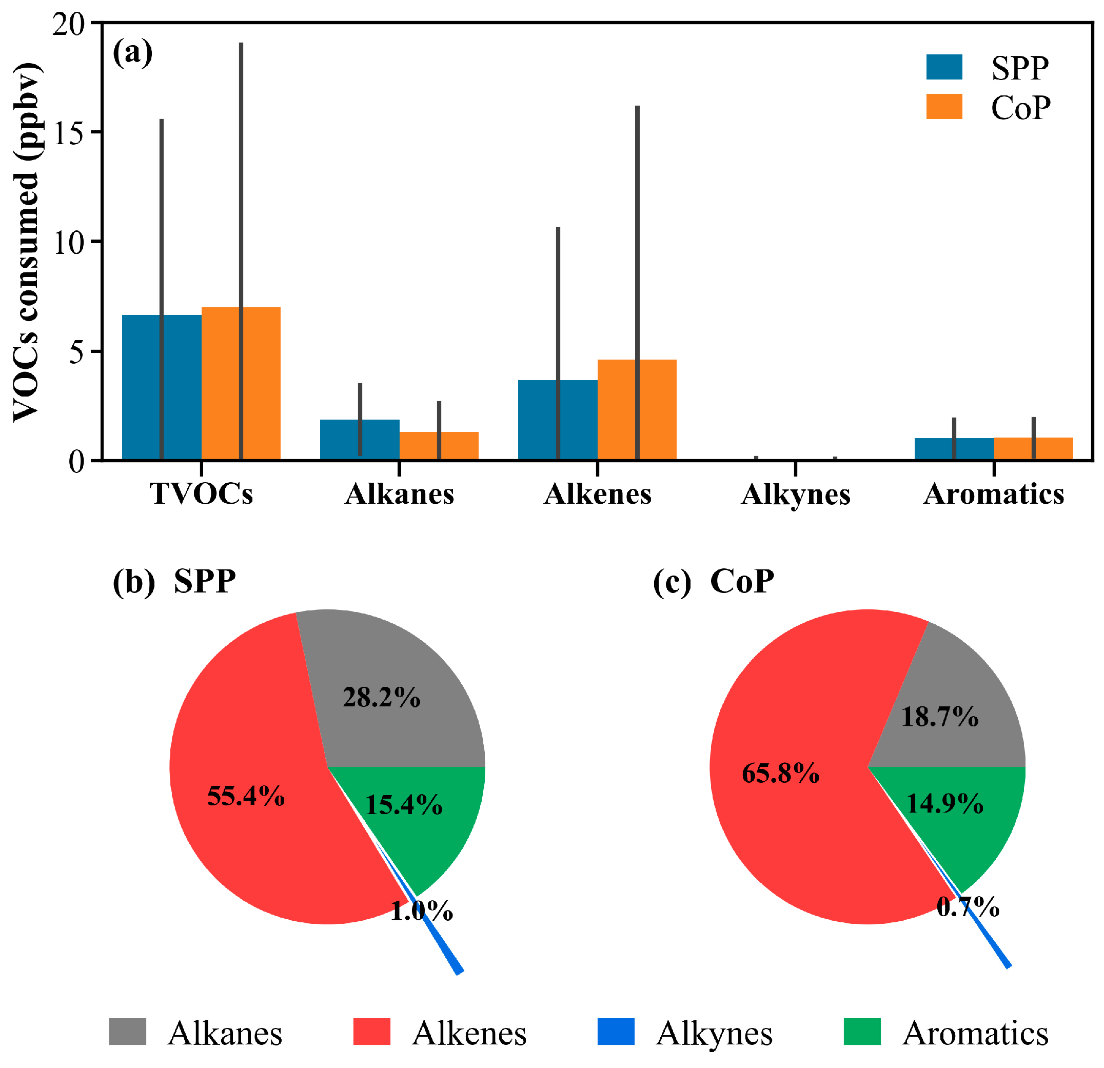
3.4. Characteristics of Consumed VOCs in Different Pollution Episodes

It is well-known that VOCs are one of the important precursors of tropospheric O3 [38]. Once VOCs are emitted by emission sources, they undergo photochemical consumption during their subsequent transport. Zhan et al. [56] reported that the photochemical consumption of VOCs is strongly associated with the formation of O3 and SOA. Thus, to further investigate the VOCs consumed and their contribution to SOA in different pollution episodes, VOC consumption was estimated based on the assumption that the oxidation of OH radicals dominate the loss of VOCs in the ambient atmosphere. A detailed description of the estimation steps can be found in Section 2.3.2.

3.4.1. Composition and Diurnal Patterns of Consumed VOCs

Figure 8 shows the average concentration and composition of the VOCs consumed during the SPP and CoP. As can be seen in Figure 8a, the total VOCs consumed during CoP (7.0 ± 12.1 ppbv) were slightly higher than those during SPP (6.6 ± 8.9 ppbv), mainly due to the high consumption of alkenes in CoP. In addition, the composition of consumed VOCs differed from the composition of measured VOCs (ranked as alkanes >> aromatics > alkenes > alkynes), and the largest proportion of the consumed VOCs consisted of alkenes (55.4–65.8%), followed by alkanes (18.7% to 28.2%), and aromatics (14.9% to 15.4%).
Figure 9 also presents the diurnal patterns of the total concentration and composition of the consumed VOCs. The consumption of VOCs exhibited different diurnal patterns in different pollution episodes. Overall, the total VOCs consumed in the two episodes showed a clear unimodal trend, with the peak occurring after the O3 peak and relatively close to the Ox peak. Meanwhile, the peak in CoP was obviously earlier than that in SPP. As for the diurnal variation in the composition of consumed VOCs (Figure 9b,c), a high percentage of alkenes appeared during the daytime, while high percentages of alkanes and aromatics occurred at night.

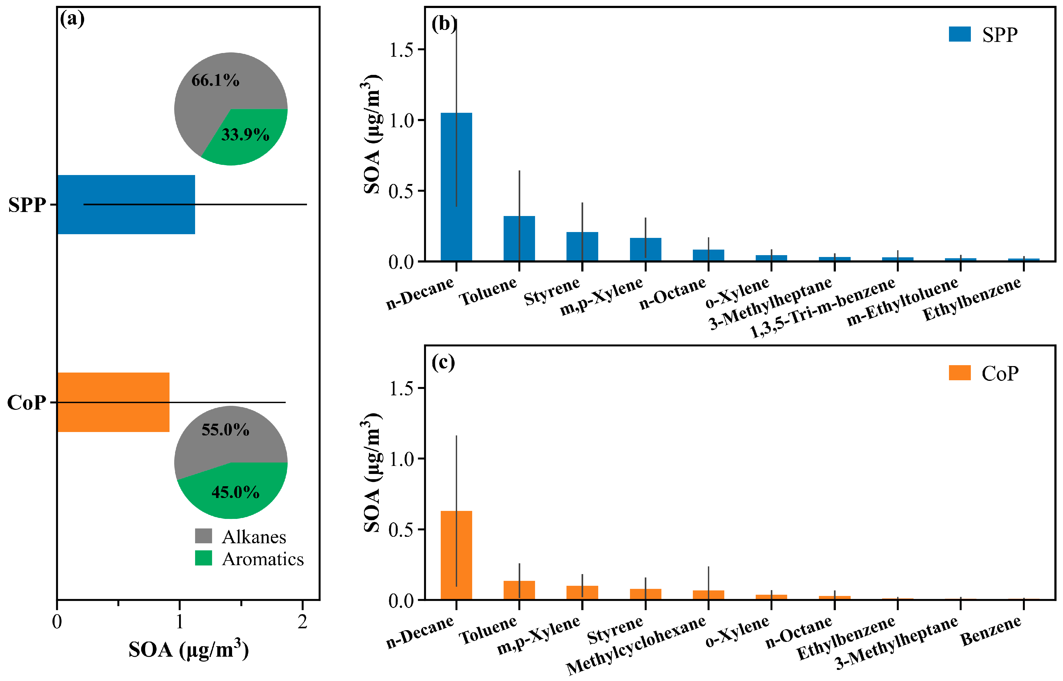
3.4.2. Estimation of SOA Based on VOC Consumption

SOA estimation based on VOC consumption can reflect the potential of VOCs to form SOA through the photochemical oxidation pathway [12]. As shown in Figure 10a, SOA that can be produced through VOC consumption in SPP and CoP were 1.1 ± 0.9 μg/m3 and 0.9 ± 0.9 μg/m3, respectively. Combined with Figure 8a, it can be seen that although the VOC consumption of CoP was higher than that of SPP, its SOA generation through VOC consumption was lower than that of SPP. This finding could be explained by the competing effects of other oxidants (e.g., NO3 radical and O3) in CoP. On the one hand, the O3 concentration of CoP was about twice that of SPP, which may enhance the formation of NO3 radicals and thus promote the NO3 oxidation of VOCs; on the other hand, the high concentration of O3 may directly lead to the O3 oxidation of VOCs. To address this issue, the formation of SOA through the different oxidation pathways of VOCs can be systematically investigated in future studies.
As shown in Figure 10b,c, the VOC species that contributed the most to SOA production according to the VOC consumption-based SOA yield method were n-decane, toluene, m,p-xylene, styrene, n-octane, o-xylene, and methylcyclohexane. A previous study conducted in Chengdu during the summer period reported that aromatic hydrocarbons, such as toluene, m,p-xylene, o-xylene, and ethylbenzene, contributed significantly to the estimated SOA potential based on the measured VOC concentrations [32]. However, our estimate of SOA based on VOC concentrations consumed by OH radicals also highlight the high contribution of high-carbon alkanes, such as n-decane and n-octane, to SOA formation. Therefore, in addition to reducing the emissions from aromatic hydrocarbons, mitigating the emissions of these high-carbon alkanes would also have a positive impact on the control of secondary organic pollution.

4. Conclusions

In this study, the formation characteristics of SOA in different types of haze pollution in Chengdu were investigated. During the observation period, a CoP occurred immediately after an SPP, and the O3 concentration in CoP was almost twice as high as that in SPP. The enhanced atmospheric oxidation during CoP resulted in a 51.2% increase in SOA concentrations as compared to the SPP. The lower measured VOC concentrations during the CoP also suggested that VOC consumption was greater in a highly oxidizing ambient atmosphere. Meanwhile, a slightly higher photochemical consumption of VOCs was derived during the CoP episode. However, the SOA produced through photochemical consumption showed a different profile as it was slightly lower in CoP. Furthermore, we found that some high-carbon alkanes (n-decane and n-octane) and aromatic hydrocarbons significantly contributed to SOA production in both pollution episodes. Thus, it is necessary to strengthen the control of these species in order to mitigate secondary organic pollution.
To some extent, our findings can help us to understand the formation of SOA in different types of pollution episodes. The biggest limitation of this study is that only one SPP episode and one CoP episode were included, which can provide a preliminary insight into SOA formation during different pollution episodes, but is not sufficient so as to provide an in-depth analysis of its causes. In the future, longer-term or multi-year measurements should be carried out to cover more pollution episodes and to further analyze the causes of high SOA concentrations in CoP episodes. Similar studies should also be conducted during the typical periods when only PM2.5 pollution or only O3 pollution is present, in order to explore the synergistic control of PM2.5 and O3 from multiple perspectives.

Supplementary Materials

The following supporting information can be downloaded at: https://www.mdpi.com/article/10.3390/atmos13111834/s1, Figure S1: Illustration of the use of the minimum R2 method (MRS) to obtain (OC/EC)pri. Table S1: SOA yields of the VOC photochemical reaction in this study.

Author Contributions

Conceptualization, X.C.; methodology, T.S. and Y.L.; data curation, M.F. and D.S., writing—original draft preparation, T.S.; writing—review and editing, X.C. and Y.W.; visualization, T.S. and S.L.; supervision, Q.T. and F.Y. All authors have read and agreed to the published version of the manuscript.

Funding

This research was funded by the National Natural Science Foundation of China (Grant No. 42175124 and 41875162) and the Chengdu Science and Technology Bureau (Grant No. 2020-YF09-00051-SN).

Institutional Review Board Statement

Not applicable.

Informed Consent Statement

Not applicable.

Data Availability Statement

Not applicable.

Acknowledgments

We are grateful for the financial support from the National Natural Science Foundation of China (No. 42175124 and 41875162) and Chengdu Science and Technology Bureau (No. 2020-YF09-00051-SN). We would also like to extend our deep gratitude to the reviewers and editors who provided valuable comments to improve the quality of the paper.

Conflicts of Interest

The authors declare no conflict of interest.

References

  1. Deng, C.; Tian, S.; Li, Z.W.; Li, K. Spatiotemporal characteristics of PM2.5 and ozone concentrations in Chinese urban clusters. Chemosphere 2022, 295, 133813. [Google Scholar] [CrossRef]
  2. Zhao, H.; Chen, K.; Liu, Z.; Zhang, Y.; Shao, T.; Zhang, H. Coordinated control of PM2.5 and O3 is urgently needed in China after implementation of the “Air pollution prevention and control action plan”. Chemosphere 2021, 270, 129441. [Google Scholar] [CrossRef]
  3. State Council of the People’s Republic of China. Air pollution Prevention and Control Action Plan 2013; State Council of the People’s Republic of China: Beijing, China, 2013.
  4. State Council of the People’s Republic of China. Three-Year Action Plan of Win the Blue Sky Defence War 2018; State Council of the People’s Republic of China: Beijing, China, 2018.
  5. Zhai, S.; Jacob, D.J.; Wang, X.; Shen, L.; Li, K.; Zhang, Y.; Gui, K.; Zhao, T.; Liao, H. Fine particulate matter (PM2.5) trends in China, 2013–2018: Separating contributions from anthropogenic emissions and meteorology. Atmos. Chem. Phys. 2019, 19, 11031–11041. [Google Scholar] [CrossRef] [Green Version]
  6. Li, K.; Jacob, D.J.; Liao, H.; Zhu, J.; Shah, V.; Shen, L.; Bates, K.H.; Zhang, Q.; Zhai, S. A two-pollutant strategy for improving ozone and particulate air quality in China. Nat. Geosci. 2019, 12, 906–910. [Google Scholar] [CrossRef]
  7. Zhao, S.; Yu, Y.; Yin, D.; Qin, D.; He, J.; Dong, L. Spatial patterns and temporal variations of six criteria air pollutants during 2015 to 2017 in the city clusters of Sichuan Basin, China. Sci. Total Environ. 2018, 624, 540–557. [Google Scholar] [CrossRef]
  8. Dai, H.; Zhu, J.; Liao, H.; Li, J.; Liang, M.; Yang, Y.; Yue, X. Co-occurrence of ozone and PM2.5 pollution in the Yangtze River Delta over 2013–2019: Spatiotemporal distribution and meteorological conditions. Atmos. Res. 2021, 249, 105363. [Google Scholar] [CrossRef]
  9. He, Y.; Li, L.; Wang, H.; Xu, X.; Li, Y.; Fan, S. A cold front induced co-occurrence of O3 and PM2.5 pollution in a Pearl River Delta city: Temporal variation, vertical structure, and mechanism. Environ. Pollut. 2022, 306, 119464. [Google Scholar] [CrossRef]
  10. Luo, Y.; Zhao, T.; Yang, Y.; Zong, L.; Kumar, K.R.; Wang, H.; Meng, K.; Zhang, L.; Lu, S.; Xin, Y. Seasonal changes in the recent decline of combined high PM2.5 and O3 pollution and associated chemical and meteorological drivers in the Beijing–Tianjin–Hebei region, China. Sci. Total Environ. 2022, 838, 156312. [Google Scholar] [CrossRef]
  11. Hallquist, M.; Wenger, J.C.; Baltensperger, U.; Rudich, Y.; Simpson, D.; Claeys, M.; Dommen, J.; Donahue, N.M.; George, C.; Goldstein, A.H.; et al. The formation, properties and impact of secondary organic aerosol: Current and emerging issues. Atmos. Chem. Phys. 2009, 9, 5155–5236. [Google Scholar] [CrossRef] [Green Version]
  12. Wang, H.; Wang, Q.; Gao, Y.; Zhou, M.; Jing, S.; Qiao, L.; Yuan, B.; Huang, D.; Huang, C.; Lou, S.; et al. Estimation of Secondary Organic Aerosol Formation During a Photochemical Smog Episode in Shanghai, China. J. Geophys. Res. Atmos. 2020, 125, e2019JD032033. [Google Scholar] [CrossRef]
  13. Li, Q.; Su, G.; Li, C.; Liu, P.; Zhao, X.; Zhang, C.; Sun, X.; Mu, Y.; Wu, M.; Wang, Q.; et al. An investigation into the role of VOCs in SOA and ozone production in Beijing, China. Sci. Total Environ. 2020, 720, 137536. [Google Scholar] [CrossRef]
  14. Wang, T.; Xue, L.; Brimblecombe, P.; Lam, Y.F.; Li, L.; Zhang, L. Ozone pollution in China: A review of concentrations, meteorological influences, chemical precursors, and effects. Sci. Total Environ. 2017, 575, 1582–1596. [Google Scholar] [CrossRef]
  15. Lu, K.; Guo, S.; Tan, Z.; Wang, H.; Shang, D.; Liu, Y.; Li, X.; Wu, Z.; Hu, M.; Zhang, Y. Exploring atmospheric free-radical chemistry in China: The self-cleansing capacity and the formation of secondary air pollution. Natl. Sci. Rev. 2019, 6, 579–594. [Google Scholar] [CrossRef] [Green Version]
  16. Wu, C.; Yu, J.Z. Determination of primary combustion source organic carbon-to-elemental carbon (OC / EC) ratio using ambient OC and EC measurements: Secondary OC-EC correlation minimization method. Atmos. Chem. Phys. 2016, 16, 5453–5465. [Google Scholar] [CrossRef] [Green Version]
  17. Guo, S.; Hu, M.; Guo, Q.; Shang, D. Comparison of Secondary Organic Aerosol Estimation Methods. Acta Chim. Sinica 2014, 72, 658–666. [Google Scholar] [CrossRef] [Green Version]
  18. Ren, H.; Hu, W.; Wei, L.; Yue, S.; Zhao, J.; Li, L.; Wu, L.; Zhao, W.; Ren, L.; Kang, M.; et al. Measurement report: Vertical distribution of biogenic and anthropogenic secondary organic aerosols in the urban boundary layer over Beijing during late summer. Atmos. Chem. Phys. 2021, 21, 12949–12963. [Google Scholar] [CrossRef]
  19. Yang, C.; Hong, Z.; Chen, J.; Xu, L.; Zhuang, M.; Huang, Z. Characteristics of secondary organic aerosols tracers in PM2.5 in three central cities of the Yangtze river delta, China. Chemosphere 2022, 293, 133637. [Google Scholar] [CrossRef]
  20. Zheng, H.; Kong, S.; Chen, N.; Niu, Z.; Zhang, Y.; Jiang, S.; Yan, Y.; Qi, S. Source apportionment of volatile organic compounds: Implications to reactivity, ozone formation, and secondary organic aerosol potential. Atmos. Res. 2021, 249, 105344. [Google Scholar] [CrossRef]
  21. Zhao, S.; Yin, D.; Yu, Y.; Kang, S.; Qin, D.; Dong, L. PM2.5 and O3 pollution during 2015–2019 over 367 Chinese cities: Spatiotemporal variations, meteorological and topographical impacts. Environ. Pollut. 2020, 264, 114694. [Google Scholar] [CrossRef]
  22. Huang, X.; Zhang, J.K.; Luo, B.; Wang, L.L.; Tang, G.Q.; Liu, Z.R.; Song, H.Y.; Zhang, W.; Yuan, L.; Wang, Y.S. Water-soluble ions in PM2.5 during spring haze and dust periods in Chengdu, China: Variations, nitrate formation and potential source areas. Environ. Pollut. 2018, 243, 1740–1749. [Google Scholar] [CrossRef]
  23. Li, L.; Tan, Q.W.; Zhang, Y.H.; Feng, M.; Qu, Y.; An, J.L.; Liu, X.G. Characteristics and source apportionment of PM2.5 during persistent extreme haze events in Chengdu, southwest China. Environ. Pollut. 2017, 230, 718–729. [Google Scholar] [CrossRef]
  24. Tian, M.; Liu, Y.; Yang, F.; Zhang, L.; Peng, C.; Chen, Y.; Shi, G.; Wang, H.; Luo, B.; Jiang, C.; et al. Increasing importance of nitrate formation for heavy aerosol pollution in two megacities in Sichuan Basin, southwest China. Environ. Pollut. 2019, 250, 898–905. [Google Scholar] [CrossRef]
  25. Song, T.; Feng, M.; Song, D.; Zhou, L.; Qiu, Y.; Tan, Q.; Yang, F. Enhanced nitrate contribution during winter haze events in a megacity of Sichuan Basin, China: Formation mechanism and source apportionment. J. Clean. Prod. 2022, 370, 133272. [Google Scholar] [CrossRef]
  26. Yang, X.; Wu, K.; Wang, H.; Liu, Y.; Gu, S.; Lu, Y.; Zhang, X.; Hu, Y.; Ou, Y.; Wang, S.; et al. Summertime ozone pollution in Sichuan Basin, China: Meteorological conditions, sources and process analysis. Atmos. Environ. 2020, 226, 117392. [Google Scholar] [CrossRef]
  27. Yang, Y.; Li, X.; Zu, K.; Lian, C.; Chen, S.; Dong, H.; Feng, M.; Liu, H.; Liu, J.; Lu, K.; et al. Elucidating the effect of HONO on O3 pollution by a case study in southwest China. Sci. Total Environ. 2021, 756, 144127. [Google Scholar] [CrossRef]
  28. Tan, Z.; Lu, K.D.; Jiang, M.Q.; Su, R.; Dong, H.B.; Zeng, L.M.; Xie, S.D.; Tan, Q.W.; Zhang, Y.H. Exploring ozone pollution in Chengdu, southwestern China: A case study from radical chemistry to O3-VOC-NOx sensitivity. Sci. Total Environ. 2018, 636, 775–786. [Google Scholar] [CrossRef]
  29. Deng, Y.; Li, J.; Li, Y.Q.; Wu, R.R.; Xie, S.D. Characteristics of volatile organic compounds, NO2, and effects on ozone formation at a site with high ozone level in Chengdu. J. Environ. Sci. 2019, 75, 334–345. [Google Scholar] [CrossRef]
  30. Kong, L.; Feng, M.; Liu, Y.; Zhang, Y.; Zhang, C.; Li, C.; Qu, Y.; An, J.; Liu, X.; Tan, Q.; et al. Elucidating the pollution characteristics of nitrate, sulfate and ammonium in PM2.5 in Chengdu, southwest China, based on 3-year measurements. Atmos. Chem. Phys. 2020, 20, 11181–11199. [Google Scholar] [CrossRef]
  31. Kong, L.; Tan, Q.W.; Feng, M.; Qu, Y.; An, J.L.; Liu, X.G.; Cheng, N.L.; Deng, Y.J.; Zhai, R.X.; Wang, Z. Investigating the characteristics and source analyses of PM2.5 seasonal variations in Chengdu, Southwest China. Chemosphere 2020, 243, 125267. [Google Scholar] [CrossRef]
  32. Xiong, C.; Wang, N.; Zhou, L.; Yang, F.; Qiu, Y.; Chen, J.; Han, L.; Li, J. Component characteristics and source apportionment of volatile organic compounds during summer and winter in downtown Chengdu, southwest China. Atmos. Environ. 2021, 258, 118485. [Google Scholar] [CrossRef]
  33. Zhao, S.; Yu, Y.; Qin, D.H.; Yin, D.Y.; Dong, L.X.; He, J.J. Analyses of regional pollution and transportation of PM2.5 and ozone in the city clusters of Sichuan Basin, China. Atmos. Pollut. Res. 2019, 10, 374–385. [Google Scholar] [CrossRef]
  34. Song, M.; Liu, X.G.; Tan, Q.W.; Feng, M.; Qu, Y.; An, J.L.; Zhang, Y.H. Characteristics and formation mechanism of persistent extreme haze pollution events in Chengdu, southwestern China. Environ. Pollut. 2019, 251, 1–12. [Google Scholar] [CrossRef]
  35. Song, M.; Tan, Q.; Feng, M.; Qu, Y.; Liu, X.; An, J.; Zhang, Y. Source Apportionment and Secondary Transformation of Atmospheric Nonmethane Hydrocarbons in Chengdu, Southwest China. J. Geophys. Res. Atmos. 2018, 123, 9741–9763. [Google Scholar] [CrossRef]
  36. Turpin, B.J.; Huntzicker, J.J. Identification of secondary organic aerosol episodes and quantitation of primary and secondary organic aerosol concentrations during SCAQS. Atmos. Environ. 1995, 29, 3527–3544. [Google Scholar] [CrossRef]
  37. Hu, W.; Hu, M.; Hu, W.-W.; Niu, H.; Zheng, J.; Wu, Y.; Chen, W.; Chen, C.; Li, L.; Shao, M.; et al. Characterization of submicron aerosols influenced by biomass burning at a site in the Sichuan Basin, southwestern China. Atmos. Chem. Phys. 2016, 16, 13213–13230. [Google Scholar] [CrossRef] [Green Version]
  38. Seinfeld, J.H.; Pandis, S.N. Atmospheric Chemistry and Physics: From Air Pollution to Climate Change; John Wiley & Sons: Hoboken, NJ, USA, 2006. [Google Scholar]
  39. Ng, N.L.; Kroll, J.H.; Chan, A.W.H.; Chhabra, P.S.; Flagan, R.C.; Seinfeld, J.H. Secondary organic aerosol formation from m-xylene, toluene, and benzene. Atmos. Chem. Phys. 2007, 7, 3909–3922. [Google Scholar] [CrossRef] [Green Version]
  40. Lim, Y.B.; Ziemann, P.J. Effects of Molecular Structure on Aerosol Yields from OH Radical-Initiated Reactions of Linear, Branched, and Cyclic Alkanes in the Presence of NOx. Environ. Sci. Technol. 2009, 43, 2328–2334. [Google Scholar] [CrossRef]
  41. Zhang, X.; Cappa, C.D.; Jathar, S.H.; McVay, R.C.; Ensberg, J.J.; Kleeman, M.J.; Seinfeld, J.H. Influence of vapor wall loss in laboratory chambers on yields of secondary organic aerosol. Proc. Natl. Acad. Sci. USA 2014, 111, 5802–5807. [Google Scholar] [CrossRef] [Green Version]
  42. Shao, M.; Wang, B.; Lu, S.; Yuan, B.; Wang, M. Effects of Beijing Olympics Control Measures on Reducing Reactive Hydrocarbon Species. Environ. Sci. Technol. 2011, 45, 514–519. [Google Scholar] [CrossRef]
  43. Wu, C.; Wang, C.; Wang, S.; Wang, W.; Yuan, B.; Qi, J.; Wang, B.; Wang, H.; Wang, C.; Song, W.; et al. Measurement report: Important contributions of oxygenated compounds to emissions and chemistry of volatile organic compounds in urban air. Atmos. Chem. Phys. 2020, 20, 14769–14785. [Google Scholar] [CrossRef]
  44. Zou, Y.; Charlesworth, E.; Wang, N.; Flores, R.M.; Liu, Q.Q.; Li, F.; Deng, T.; Deng, X.J. Characterization and ozone formation potential (OFP) of non-methane hydrocarbons under the condition of chemical loss in Guangzhou, China. Atmos. Environ. 2021, 262, 118630. [Google Scholar] [CrossRef]
  45. Yuan, B.; Hu, W.W.; Shao, M.; Wang, M.; Chen, W.T.; Lu, S.H.; Zeng, L.M.; Hu, M. VOC emissions, evolutions and contributions to SOA formation at a receptor site in eastern China. Atmos. Chem. Phys. 2013, 13, 8815–8832. [Google Scholar] [CrossRef] [Green Version]
  46. Wang, H.; Tian, M.; Chen, Y.; Shi, G.; Liu, Y.; Yang, F.; Zhang, L.; Deng, L.; Yu, J.; Peng, C.; et al. Seasonal characteristics, formation mechanisms and source origins of PM2.5 in two megacities in Sichuan Basin, China. Atmos. Chem. Phys. 2018, 18, 865–881. [Google Scholar] [CrossRef] [Green Version]
  47. Sbai, S.E.; Li, C.; Boreave, A.; Charbonnel, N.; Perrier, S.; Vernoux, P.; Bentayeb, F.; George, C.; Gil, S. Atmospheric photochemistry and secondary aerosol formation of urban air in Lyon, France. J. Environ. Sci. 2021, 99, 311–323. [Google Scholar] [CrossRef] [PubMed]
  48. Li, J.; Deng, S.; Li, G.; Lu, Z.; Song, H.; Gao, J.; Sun, Z.; Xu, K. VOCs characteristics and their ozone and SOA formation potentials in autumn and winter at Weinan, China. Environ. Res. 2022, 203, 111821. [Google Scholar] [CrossRef] [PubMed]
  49. Shi, J.; Bao, Y.; Xiang, F.; Wang, Z.; Ren, L.; Pang, X.; Wang, J.; Han, X.; Ning, P. Pollution Characteristics and Health Risk Assessment of VOCs in Jinghong. Atmosphere 2022, 13, 613. [Google Scholar] [CrossRef]
  50. Niu, Y.; Yan, Y.; Chai, J.; Zhang, X.; Xu, Y.; Duan, X.; Wu, J.; Peng, L. Effects of regional transport from different potential pollution areas on volatile organic compounds (VOCs) in Northern Beijing during non-heating and heating periods. Sci. Total Environ. 2022, 836, 155465. [Google Scholar] [CrossRef]
  51. Zhang, L.; Li, H.; Wu, Z.; Zhang, W.; Liu, K.; Cheng, X.; Zhang, Y.; Li, B.; Chen, Y. Characteristics of atmospheric volatile organic compounds in urban area of Beijing: Variations, photochemical reactivity and source apportionment. J. Environ. Sci. 2020, 95, 190–200. [Google Scholar] [CrossRef]
  52. Kumar, A.; Singh, D.; Kumar, K.; Singh, B.B.; Jain, V.K. Distribution of VOCs in urban and rural atmospheres of subtropical India: Temporal variation, source attribution, ratios, OFP and risk assessment. Sci. Total Environ. 2018, 613–614, 492–501. [Google Scholar] [CrossRef]
  53. Zhang, Y.; Yin, S.; Yuan, M.; Zhang, R.; Zhang, M.; Yu, S.; Li, Y. Characteristics and source apportionment of ambient VOC in spring in Zhengzhou. Environ. Sci. 2019, 40, 4372–4381. [Google Scholar] [CrossRef]
  54. Yan, Y.; Peng, L.; Li, R.; Li, Y.; Li, L.; Bai, H. Concentration, ozone formation potential and source analysis of volatile organic compounds (VOCs) in a thermal power station centralized area: A study in Shuozhou, China. Environ. Pollut. 2017, 223, 295–304. [Google Scholar] [CrossRef] [PubMed]
  55. Zheng, H.; Kong, S.; Xing, X.; Mao, Y.; Hu, T.; Ding, Y.; Li, G.; Liu, D.; Li, S.; Qi, S. Monitoring of volatile organic compounds (VOCs) from an oil and gas station in northwest China for 1 year. Atmos. Chem. Phys. 2018, 18, 4567–4595. [Google Scholar] [CrossRef] [Green Version]
  56. Zhan, J.; Feng, Z.; Liu, P.; He, X.; He, Z.; Chen, T.; Wang, Y.; He, H.; Mu, Y.; Liu, Y. Ozone and SOA formation potential based on photochemical loss of VOCs during the Beijing summer. Environ. Pollut. 2021, 285, 117444. [Google Scholar] [CrossRef] [PubMed]
Figure 1. The location of the sampling site in urban areas of Chengdu.
Atmosphere 13 01834 g001
Figure 2. Scatterplot of measured m, p-xylene with ethylbenzene (a) and diurnal variation of the m, p-xylene/ethylbenzene ratios (b). The red dashed line represents the m, p-xylene/ethylbenzene initial emission ratio estimated by the regression of nighttime concentrations; the blue dashed line represents the initial ratio estimated by the 90th percentile method. The black line and grey areas are the mean and standard deviation, respectively.
Atmosphere 13 01834 g002
Figure 3. Time series of PM2.5 (a,b) and its carbonaceous components (c), O3 (a,b), VOCs (d), other gaseous pollutants (e), and meteorological parameters (f,g). The grey and yellow areas represent the SPP and CoP episodes, respectively.
Atmosphere 13 01834 g003
Figure 4. Scatter plots of the SOA and PM2.5 concentrations during different pollution episodes. (a) for the whole period, (b) for the SPP episode, and (c) for the CoP episode. The red dashed line in each subplot is the linear regression line of the scatter plot.
Atmosphere 13 01834 g004
Figure 5. Diurnal patterns of different carbonaceous aerosols (a,b), O3 (c), T (d) and RH (e) in different pollution episodes. The solid line and shaded areas are the mean and standard deviation, respectively.
Atmosphere 13 01834 g005
Figure 6. The VOC composition (a,c) and top 10 abundant species (b,d) in different pollution episodes. The error line on each bar corresponds to the standard deviation.
Atmosphere 13 01834 g006
Figure 7. Diurnal patterns of VOCs (ae), NOx (f), O3 (g), and Ox (h) in different pollution episodes. The solid line and shaded areas are the mean and standard deviation, respectively.
Atmosphere 13 01834 g007
Figure 8. Concentration (a) and composition (b,c) of consumed VOCs in different pollution episodes. The error line on each bar corresponds to the standard deviation.
Atmosphere 13 01834 g008
Figure 9. Diurnal pattern of TVOCs (a) and chemical composition (b,c) of consumed VOCs in different pollution episodes. The solid line and shaded areas in figure (a) are the mean and standard deviation, respectively.
Atmosphere 13 01834 g009
Figure 10. Comparison of SOA generation estimated from consumed VOCs in different pollution episodes (a) and the top ten 10 VOCs species forming SOA by photochemical oxidation (b,c). The error line on each bar corresponds to the standard deviation.
Atmosphere 13 01834 g010
Table 1. Statistical summary (mean ± std) of measured air pollutants, carbonaceous components in PM2.5, VOC, and meteorological parameters in this study.
Whole Period
(1–30 April 2019) 1
SPP
(16–20 April 2019) 1
CoP
(22–27 April 2019) 1
Air pollutants
PM2.5 (μg/m3)40.6 ± 22.953.2 ± 24.755.3 ± 19.6
O3 (μg/m3)59.9 ± 47.854.3 ± 46.797.7 ± 63.9
MDA8 O3 (μg/m3)106.5 ± 42.6109.2 ± 27.6170.0 ± 33.9
NO2 (μg/m3)41.2 ± 22.346.1 ± 17.143.0 ± 23.6
NO (μg/m3)10.0 ± 18.19.4 ± 11.07.5 ± 9.9
CO (mg/m3)0.7 ± 0.20.8 ± 0.20.7 ± 0.2
Carbonaceous components in PM2.5
POA (μg/m3)5.3 ± 3.76.8 ± 4.16.6 ± 3.1
SOA (μg/m3)5.6 ± 3.24.3 ± 3.26.5 ± 2.6
EC (μg/m3)1.1 ± 0.81.5 ± 0.91.4 ± 0.7
Measured VOCs
TVOCs (ppbv) 236.2 ± 19.844.8 ± 16.134.4 ± 20.0
Alkanes (ppbv)24.5 ± 14.131.1 ± 11.421.8 ± 14.2
Alkenes (ppbv)4.1 ± 1.74.4 ± 1.34.3 ± 1.7
Alkynes (ppbv)3.1 ± 2.24.5 ± 2.93.2 ± 1.9
Aromatics (ppbv)4.4 ± 3.14.8 ± 2.15.0 ± 3.4
Meteorological parameters
T (°C)22.1 ± 4.921.5 ± 3.227.7 ± 3.4
Tmax (°C) 326.3 ± 5.025.7 ± 1.932.2 ± 1.9
RH (%)63.9 ± 16.172.4 ± 10.754.6 ± 10.8
WS (m/s)1.1 ± 0.91.0 ± 0.71.2 ± 1.2
1 The corresponding dates for the whole period, SPP, and CoP. 2 The mixing ratios of total VOCs. 3 The daily maximum temperature.
Table 2. Ratios of different VOC species pairs in this study for different pollution episodes and other research works.
Benzene/TolueneIsopentane/n-Pentane
This study
SPP (2019.4.16–4.20)0.86 ± 1.57 12.65 ± 0.70 2
CoP (2019.4.22–4.27)0.75 ± 0.60 13.42 ± 1.12 2
Previous studies
Solvent usage0.00–0.20 3
Biomass burning2.50 3
Vehicle emission0.56–0.60 32.93 4
Coal combustion1.05–2.20 30.56–0.80 4
Natural gas 0.82-0.89 5
Liquid gasoline 1.50–3.00 5
Fuel volatilization 1.84–4.46 5
1 Ratios of benzene to toluene in this study. 2 Ratios of isopentane to n-pentane in this study. 3 Ratios of benzene to toluene in different emission sources, with reference to Zhang and co-authors [53]. 4 and 5 Ratios of isopentane to n-pentane in different emission sources, with reference to Yan and co-authors [54], and Zheng and co-authors [55], respectively.
Publisher’s Note: MDPI stays neutral with regard to jurisdictional claims in published maps and institutional affiliations.

