Article

A PM2.5 Concentration Prediction Model Based on CART–BLS

1
School of Electrical Engineering, Yancheng Institute of Technology, Yancheng 224051, China
2
School of Automation, Hangzhou Dianzi University, Hangzhou 310018, China
3
Zhejiang Zhengtai Zhongzi Control Engineering Co., Ltd., Hangzhou 310018, China
*
Authors to whom correspondence should be addressed.
Atmosphere 2022, 13(10), 1674; https://doi.org/10.3390/atmos13101674
Submission received: 19 September 2022 / Revised: 11 October 2022 / Accepted: 11 October 2022 / Published: 13 October 2022
(This article belongs to the Special Issue Air Quality Prediction and Modeling)

Abstract

:
With the development of urbanization, the hourly PM2.5 concentration in the air is constantly changing. In order to improve the accuracy of PM2.5 prediction, a prediction model based on the Classification and Regression Tree (CART) and Broad Learning System (BLS) was constructed. Firstly, the CART algorithm was used to segment the dataset in a hierarchical way to obtain a subset with similar characteristics. Secondly, the BLS model was trained by using the data of each subset, and the validation error of each model was minimized by adjusting the window number of the mapping layer in the BLS network. Finally, for each leaf in the tree, the global BLS model and the local BLS model on the path from the root node to the leaf node are compared, and the model with the smallest error is selected. The data collected in this paper come from the Chine Meteorological Historical Data website. We selected historical data from the Huaita monitoring station in Xuzhou city for experimental analysis, which included air pollutant content and meteorological data. Experimental results show that the prediction effect of the CART–BLS model is better than that of RF, V-SVR, and seasonal BLS models.

1. Introduction

PM2.5 in the air can cause harm to organisms and human health [1,2]. Now, many studies have confirmed that PM2.5 can damage the respiratory and cardiovascular systems, and increase the incidence of asthma, lung cancer, and cardiovascular diseases [3]. Therefore, the CART–BLS network we constructed is of great significance for predicting the PM2.5 content in the air. At present, the problem of predicting the concentration of PM2.5 in the air has been a great concern of domestic and foreign scholars, and a series of prediction models have been proposed.
PM2.5 prediction models can be broadly classified into two types: deterministic models and statistical models. Deterministic models, called chemical transport models (CTMS), focus on understanding the potentially complex interactions between meteorology, chemistry, and emissions. The most widely used air pollution chemical transport model is the Community Multiscale Air Quality (CMAQ) model [4] developed by the US Environmental Protection Agency. In order to improve the reliability of CMAQ in accurately predicting atmospheric component concentrations, many studies have applied pollution transport and trajectory methods. Although they improved the transport modeling and simulation trajectories in CMAQ, there are still cases where there is a significant deviation for higher component concentrations [5]. The construction of the statistical model depends on our collected dataset, and it can verify the relationship between PM2.5 and other variables. The statistical model has the characteristics of straightforward modeling, fast modeling speed, and low economic cost. Accordingly, statistical models have attracted extensive attention. The statistical models of PM2.5 concentration are variable. Statistical models include linear and generalized regression [6], nonlinear regression, autoregressive integrated moving average [7], hidden Markov, random forest, and support vector regression models. The linear model further simplifies the prediction model and optimizes each index of particulate matter content in the air. In Latin America, Brazil is the first country to perform air quality forecasting through linear models and neural networks [8]. Zhai [9] et al. adopted a multiple linear regression model. This model takes Shijiazhuang City as the experimental object to construct the spatial distribution model of PM2.5 concentration. The results of this method show that the PM2.5 concentration progressively expands from west to east, and the municipal PM2.5 concentration is the highest, with strong regional characteristics [10]. Haoyu Teng et al. used regression analysis to forecast PM2.5. The data of Nanjing and Jilin were selected for research to further broaden the data characteristics and obtain a linear regression model of wind, temperature, CO, PM10, NO2, and other factors. Dong [11] proposed a PM2.5 inference model based on support vector machines [12,13]. This method proposes the concept of point of interest and uses the monitoring data around the point of interest to forecast the PM2.5 of the point of interest. Since the annotation of points of interest predominantly relies on manual selection, there are many locations that have great demand for air quality reports, and the data collection of these locations is relatively complete. The prediction accuracy of the model is also higher. Deters [14] et al. used boosted tree model and a support vector machine model to predict PM2.5 concentration. Although fewer data features (precipitation, wind direction, and speed) were used for prediction, better results were obtained. This experiment shows that the boosted tree model has certain advantages for dealing with linear problems, and the prediction effect is better than a single support vector machine. Since linear models do not understand feature interactions in the dataset and simplify the relationship between air pollutant concentrations and predictors. This paper introduces the Classification and Regression Trees (CART). The CART can generate easy-to-understand rules and is not computationally expensive. The CART also has the characteristics of fast training speed and prediction speed. In this paper, the CART is used to segment the dataset, and PM2.5 is divided into several subsets with similar characteristics.
Due to the limited expression ability of the linear model, the nonlinear model is constructed by adding an activation function on the basis of the linear model. Cobourn [15] proposed the method of combining nonlinear regression and reverse trajectory concentration. This method can effectively measure the maximum value of PM2.5 in a day. The concept of PM24 (24-h PM2.5 trajectory concentration) is defined in the model, which avoids the problem of missing values to a certain extent. The model further improves prediction accuracy. The model uses weather data as input features to predict the value of PM2.5. The impact of other atmospheric pollutants (CO, SO2, etc.) on PM2.5 is not considered. Zhang [16] et al. optimized the neural network model by adjusting the number of units in the hidden units in the BP network. This experiment proves that different numbers of hidden neurons have a big influence on accuracy. In the process of building the model, only part of the geographical factors’ influence on PM2.5 was considered, and a neural network model was established accordingly. The model does not fully use geographic factors, nor does it take into account meteorological factors and other pollutants. Bolin Liu [17] et al. further processed the BP network. They optimized the network with the help of the genetic algorithm. Compared with the unoptimized BP neural network, the model has better prediction performance. Chen [18] et al. established a grayscale prediction model to forecast the hourly concentrations of PM2.5 and PM10 in Taichung City, Taiwan Province. Compared with the BP neural network, Chen found that the prediction influence of the grayscale prediction model is superior to that of the BP neural network. Neural network models are also widely used to predict PM2.5 concentrations because of their ability to detect complex underlying nonlinear relationships. However, neural network models require considerable expertise to tune the parameters, so the training process is time-consuming. Therefore, Junlong Chen [19] et al. proposed a network architecture that only increases the network width. It’s called the Broad Learning System (BLS). The BLS can reduce the complexity of deep networks and improve their efficiency to a certain extent. Compared with the deep structure, for better training efficiency, the BLS network has undergone some changes in the hierarchical structure [20,21] or ensemble [22,23,24,25,26]. The BLS does not need to adjust parameters, and the network has a simple structure, fast training speed, and high accuracy.
Due to diurnal and seasonal changes, PM2.5 has multiple variation patterns [27]. McKendry [28] proposed that a hybrid model and a local multilayer perceptron (MLP) may outperform a single global MLP for the prediction of air pollutant concentrations. Hybrid models are models formed by combining several different models. Inchoon Yeo [29] et al. proposed a deep learning model that combines convolutional neural networks and gated recurrent units with groups of neighboring sites to accurately predict PM2.5 concentrations at 25 sites in Seoul, South Korea. Compared with the method that only uses the meteorological and air quality data of one target station to predict the PM2.5 concentration of 25 monitoring stations in Seoul, the proposed method uses the adjacent near-infrared stations based on geographical correlation as a polygon group, which effectively improves the prediction accuracy of PM2.5. Songzhou Li et al. proposed a hybrid model of AC-LSTM [30,31]. The model not only used air pollutants, but also added meteorological information and PM2.5 data from nearby air quality monitoring stations, further expanding the experimental data. The model also further improves prediction accuracy. The data classification on the local model is more granular than the mixed model. In order to monitor and estimate PM2.5 concentration, Chiou-Jye [32] et al. proposed a model combining a convolutional neural network (CNN) and long short-term memory network (LSTM). The data index of air pollutants in Beijing is used as the dataset, which includes PM2.5 concentration, cumulative wind speed, and cumulative rain hours. In this experiment, the information of the past 24 h of these factors is used to predict the PM2.5 concentration for the next hour. The model has a good effect on predicting PM2.5 concentration. Celis [33] et al. designed an air quality prevention and warning system for air pollution in Latin America. They compared three machine learning models (SVM, LSTM, and 1D-BDLM) and found that the 1D-BDLM model had the highest prediction accuracy and was able to effectively predict behavior, measurements, and air quality alerts. Habibi [34] et al. proposed an unsupervised clustering method to find high pollution areas. Although this method cannot be used to predict model results, it provides a predictable idea. First, the data are clustered to find data with similar characteristics, and then the data are learned and modeled. This method needs to divide an area into grids of uniform size, then determine the size of the grid through experiments, and perform data analysis in each grid. In this paper, the global model is trained on the dataset of air pollutants that we collected. Similarly, the data trained by the local model are a subset of the total data after the CART classification. Generally speaking, since the data required for training are divided into different ranges, there are many types of models to be trained. Thus, there is a risk of underfitting for the global model and overfitting for the local model. Therefore, this paper constructs the CART–BLS model to solve this kind of problem. After the model uses the CART to divide the dataset, each node has its own dataset. The BLS network is then trained using the dataset for each node. Experiments show that the BLS has higher prediction accuracy and faster training speed.
The contributions of this paper are as follows:
(1)
CART algorithm has good performance in dealing with data classification. BLS network has the advantages of high prediction accuracy, fast operation speed and simple structure. We combined the advantages of both to propose the CART-BLS model.
(2)
We used the CART algorithm to optimize the data set so that the data has a more detailed range and avoid the confusion of the data.
(3)
It is proved that the prediction accuracy of the CART–BLS model is high.
The organization of the full text is as follows: The first part introduces the model for predicting PM2.5 concentrations as well as the BLS network. The second part introduces the CART–BLS model and explains its principle. The third part verifies the model experimentally and compares several models. The fourth part draws the final conclusion.

2. Methods

2.1. CART Algorithm

A decision tree is a process of classifying and regressing the raw data we collect. A decision tree contains three algorithms. They are the ID3 algorithm, C4.5 algorithm, and the CART algorithm, respectively. The CART algorithms fall into two categories. One of them is the classification tree and the other is the regression tree. For the classification tree, the Gini coefficient is used as the classification index. In the case of regression trees, MSE serves as a regression index. Firstly, the regression tree splits into the root node as the starting point of the algorithm. Secondly, it splits into two parts based on the starting point, and each part continues to split according to the splitting rules. Finally, the stop condition is reached to end the splitting, and we also acquire the required data subset. For regression trees, the purpose of splitting the dataset is to minimize the expectation and variance of the two subsets. The formula is:
min j , c 1 m ( k S L ( y k y ^ L ) 2 + k S R ( y k y ^ R ) 2 ) ,
where S L = { i | x i j c , i = 1 , 2… , m } , S R = { i | x i j > c , i = 1 , 2… , m } , and j { 1 , 2… , n } . Here S L on behalf of the training index set of the left subtree node, and S R on behalf of the training index set of the right subtree node. y ^ L , y ^ R are the average in the left and right subsets, respectively. In the case of decision trees, pruning is often used to simplify the decision tree model and prevent overfitting.

2.2. BLS

The BLS is built on the basis of Random Vector Functional Link Neural Networks. On the one hand, the BLS network has feature nodes formed by feature maps. On the other hand, enhancement nodes are introduced to ensure the stability of the BLS. The BLS has the characteristics of easy to grasp framework, short time consumption, and high precision. It has good application prospects in small and medium datasets. The BLS structure is shown in Figure 1 [12]. In the BLS algorithm, the core that we need to calculate is the total pseudo-inverse matrix of the whole network. Before that, we need to perform feature mapping on the input data X. We obtain the ith set of mapped features Z i using formula φ i ( x ω e i + β e i ) , where ω e i and β e i do not need to be set manually. Their values are generated by the network. Then after mapping the features, we can obtain the result of n sets of mapped feature nodes is Z n [ Z 1 , , Z n ] . Similarly, for enhanced nodes, the mth group of enhanced nodes can be denoted as H m = ξ m ( z n ω h m + β h m ) . Therefore, the result for the m group of enhanced nodes can be expressed as H m [ H 1 , , H m ] . Therefore, the output of the BLS can be denoted as
Y = [ Z 1 , , Z n | ξ ( Z n ω h 1 + β h 1 ) , , ξ ( Z n ω h m + β h m ) ] ω m = [ Z 1 , , Z n | H 1 , , H m ] ω m , = [ Z n | H m ] ω m
where ω m is the connection weight of the BLS, which can be obtained by formula ω m = [ Z n | H m ] + Y .

2.3. CART–BLS

In order to predict the concentration of PM2.5, a new prediction model combining the CART and the BLS was proposed based on the original prediction model. The model algorithm for constructing the CART–BLS includes the following steps:
  • (1) Build the CART tree. We use the CART algorithm to train our collected data. The data build a tree in layers. Since the depth of the tree may be affected by outliers, it is necessary to set the maximum depth of the tree when building the regression tree. Each node in the partitioned tree has its own training set. We need to train a local model on each child node, so we need to set a minimum number of samples on each child node to ensure that there are enough data samples for training the local model.
  • (2) Use the relevant samples to train the BLS. Before training the BLS, we first classify the data on each node divided by the CART and then use these node samples to train the BLS parameters. The model is globally trained using the data samples of the root node. The root node data are used as the training set data, and the data on each leaf node are used as the verification data to determine the model parameters separately. Local model training of the BLS uses internal node data samples of decision trees. The internal node data are used as training data, and the leaf node data with the internal node as the root node are used as verification data. A local model is trained on each leaf node using its own data samples.
  • (3) Compare the global and local BLS models. For the global model, we compare the prediction performance of several global models at the root node. For local models, we compare the prediction effects of several local models on leaf nodes. With this in mind, we select the optimal prediction model.

3. Data and Experimental Results

3.1. Data

In the project study, the dataset was constructed from meteorological data of Xuzhou City, Jiangsu Province, China. Since China is in a period of rapid development, specifically in the urbanization process, the consumption rate of various energy sources is gradually accelerating. At the same time, the increase in automobiles has also led to an increase in vehicle exhaust emissions. As a result, the pollutants in the air also increase. In recent years, due to the gradual increase in the utilization rate of clean energy, the air pollution problem has also been alleviated, but the air pollution problem still exists.
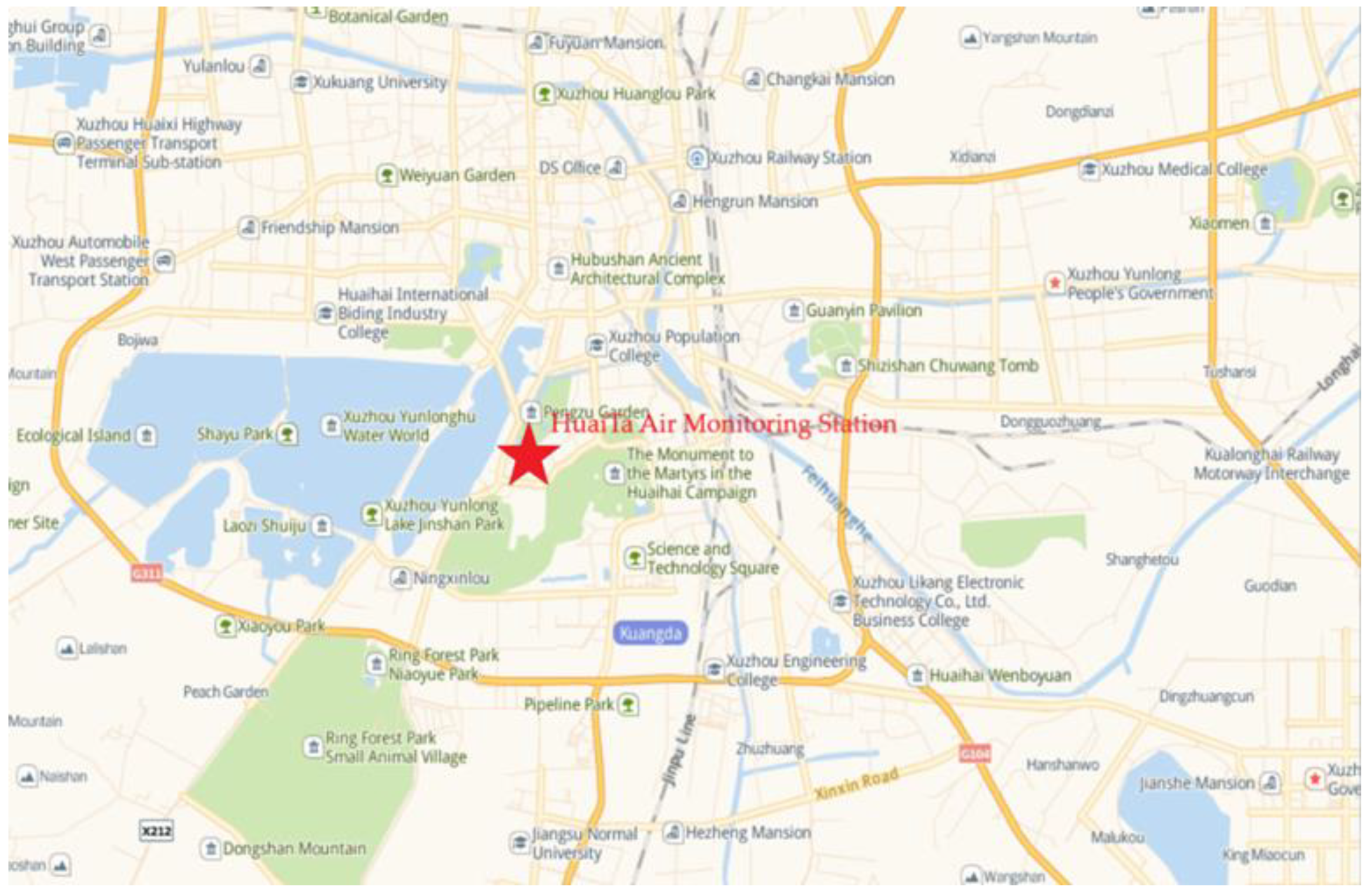
In order to detect air pollution levels, air pollution monitoring stations are established in most cities in China. These monitoring stations automatically record the air pollution (PM2.5, PM10, CO, NO2, SO2, O3) concentrations every hour. In Xuzhou, there are eight monitoring stations: Taoyuan Road, Huaita, Tongshan District Admissions Office, Academy of Agricultural Sciences, Daquan Street, Xincheng District, Yellow River New Village, and Gulou District Government, as shown in Figure 2.
The data of this subject consist of the air pollution data collected from the Huaita testing site. The data range of the dataset is from 1 January 2015 to 31 December 2021. The dataset is constructed using hourly meteorological parameters. The models involved were developed using Python 3.9.7. These experiments were performed on a computer with Windows 10 64-bit operating system running on an Intel Core(TM) i7-11800H @ 2.30GHz with 16 GB of RAM.
In data processing [35], missing values often occur, especially when performing statistical analysis on large amounts of data. Because the actual data acquisition system often has loopholes, some valuable information is lost, i.e., for missing values generated for a certain time point or time period (data not recorded by monitoring stations). For the missing data of a single point, the average value of the context data is used for data filling. For the missing data in a certain period of time, a multivariate interpolation method is used to fit the missing values into the representation function of other features, the feature prediction column is designated as the output column, and the other feature columns are used as input variables.

3.2. RF Selection Input Variable

The project dataset includes data on six air pollutants and some meteorological data. Table 1 shows the characteristic variables of the dataset. Where DPT is the dew point temperature, WD is the wind direction, and WS is the wind degree.
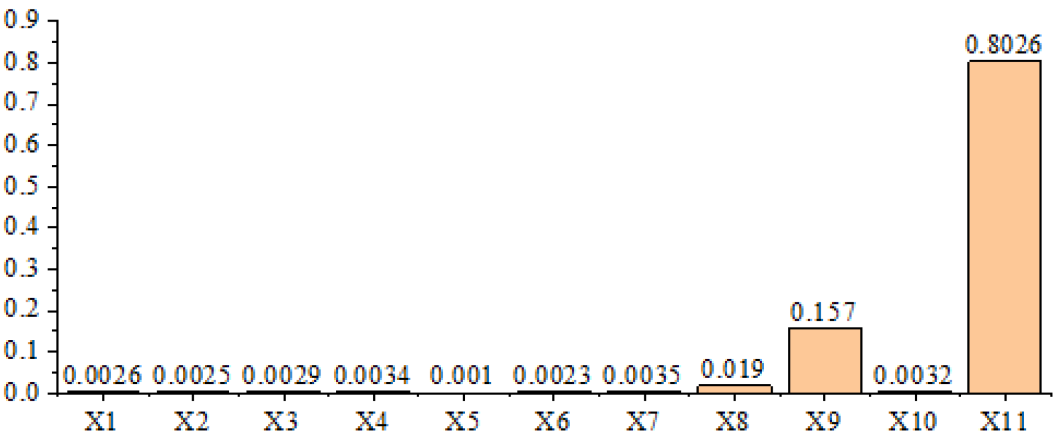
Due to the wide variety of data in the dataset, we employed a random forest algorithm to select variables that are more important for air pollution indicators. The selected variables are used as the input data of the training set. Five cross-validation methods were used to evaluate the input variables. The horizontal axis of the figure below represents the name of the variable, and the vertical axis represents the importance percentage of each variable in the overall variable. As shown in Figure 3, the PM2.5 variable has the highest percentage of the overall variable importance, reaching 80.26%, followed by PM10, accounting for 15.7%. Therefore, when training the dataset, we chose the PM2.5 variable as the input data for the training set.
For the analysis of multicollinearity, we introduce the index of Variance Inflation Factor(VIF) [36,37] based on the original analysis. For VIF, the formula is as follows:
V I F = 1 1 R i 2
Here, R i represents the negative correlation coefficient of the regression analysis of the independent variable Xi on the remaining independent variables. The larger the VIF value, the more obvious the collinearity problem, and 10 is usually used as the judgment boundary. When VIF < 10, there is no multicollinearity; when 10 <= VIF < 100, there is strong multicollinearity; when VIF >= 100, there is severe multicollinearity. The VIF values of the input vector are shown in Table 2 below.
It can be seen that except for air pressure and CO, which are beyond the bounds, the rest of the variables are within the bounds. However, for this experiment, the variable we need is PM2.5, whose VIF is 9.47 < 10, so it can be judged that there is no multicollinearity problem and it will not affect the results.

3.3. Splitting the Dataset Using the CART Decision Tree

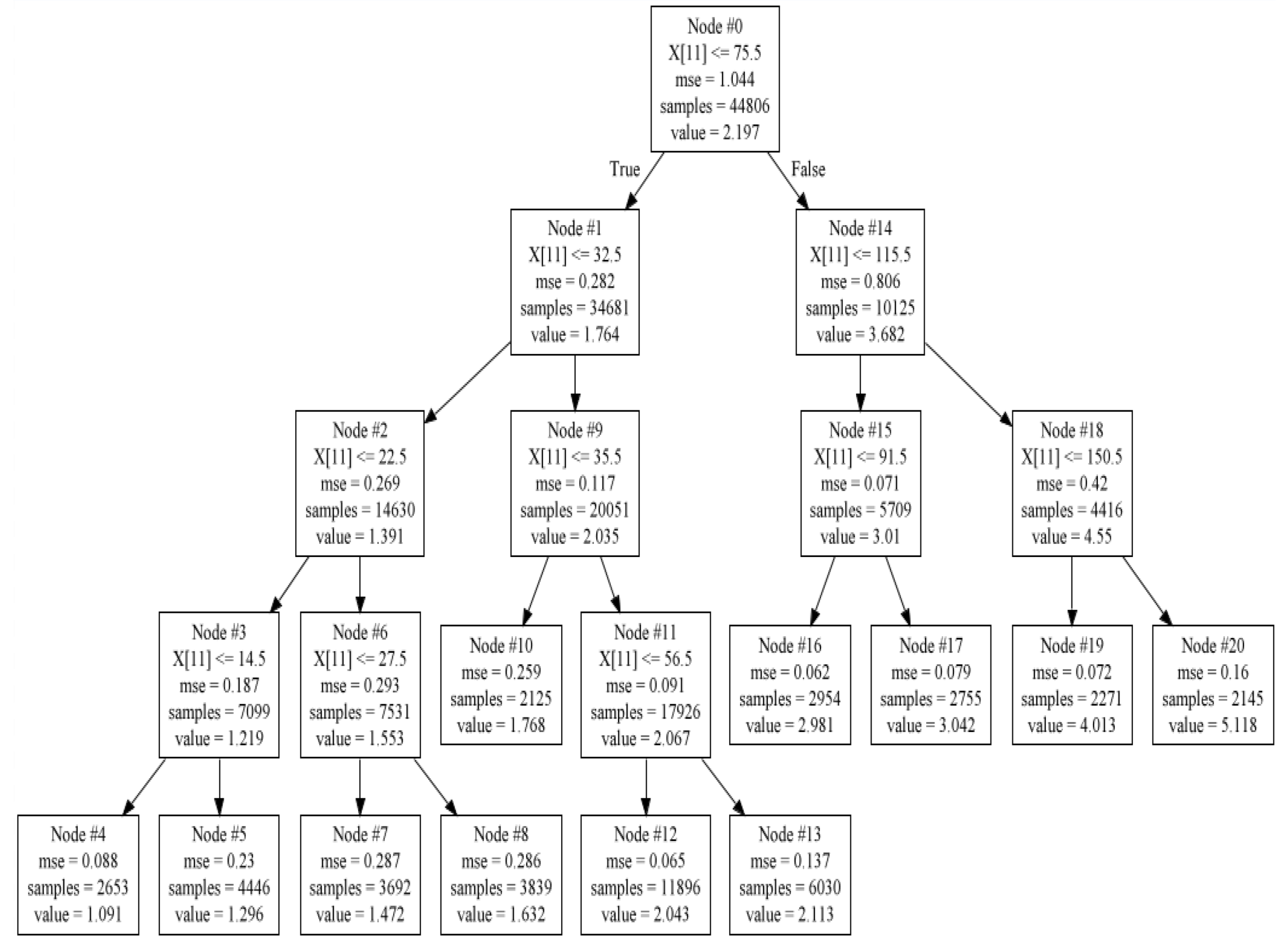
First, according to the CART node segmentation principle, we divided the collected data into a training set and a test set and selected the most important PM2.5 indicator as the input feature. Then, the CART decision tree is constructed by using the training set, and the dataset is divided to obtain the multi-modal structure of PM2.5. When training the CART algorithm, in order to ensure that there are enough data for training the BLS network, we set the amount of sample data to at least 2000 when building the tree model. In addition, due to the high time complexity of the decision tree and the problem of easy overfitting, it is necessary to prune the decision tree when constructing the decision tree. Therefore, in this experiment, we set the maximum depth of the tree to 4.
The model tree obtained in this experiment is shown in Figure 4. Divide the PM2.5 variable to obtain multiple subsets with similar characteristics.

3.4. Prediction Model Based on CART–BLS

The proposed predictive model is trained using the CART decision tree partitioned dataset. As can be seen from the above figure, after the CART splitting, each node has its own data sample. In the generated decision tree, the types of nodes can be divided into root nodes, internal nodes, and terminal nodes (leaf nodes). We use different training methods for each type of node. The data samples of the root node are the total dataset, so the global model is trained using the root node. We use the data of the root node as the training set and the data of different leaf nodes as the validation set to determine the parameters and validation errors of the proposed width learning network. In this experiment, root mean square error (RMSE) [38] is used as the criterion to verify the experimental results. Its formula is
R M S E = 1 l i = 1 l ( y i y ^ i ) 2 ,
where y ^ i is the predicted value. For internal nodes, we use the data of the internal node as the training set and the data of different nodes with the internal node as the root node as the validation set. We use this data to determine the parameters and validation errors of the wide learning network. On the terminal node, that is, the leaf node, we use the data samples on the node to train the model, dividing the data into two parts—training set and validation set—and using this data to determine the parameters and validation errors of the width learning network.
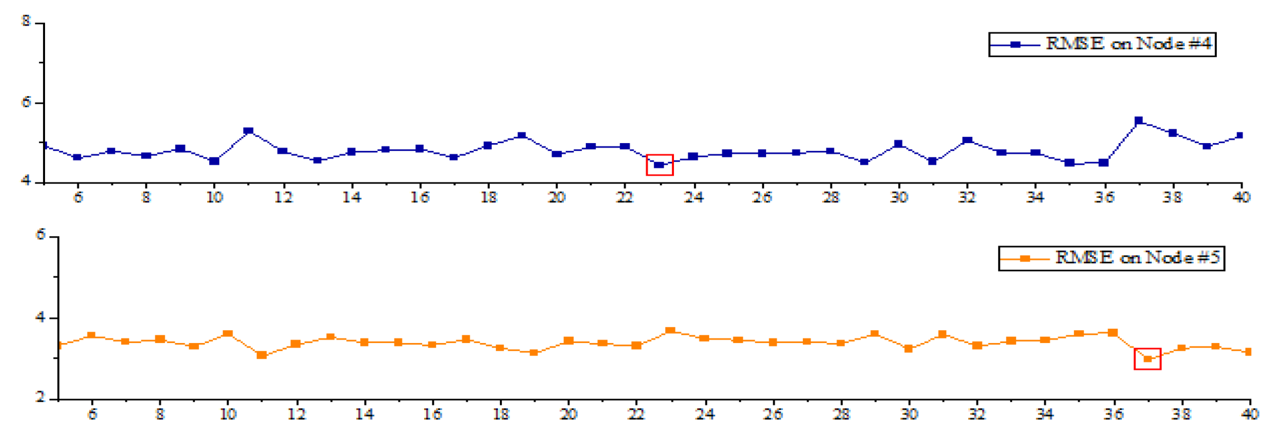
We train the BLS separately using the node data and obtain the training results of the global model and the local model. As shown in Figure 5, all nodes are organized in a hierarchical manner. To clearly express the information in the node, BLS # 4 # 3 is an example. What BLS # 4 # 3 means is to train node #4 on node #3, and the following values represent the best number of windows and the smallest validation error. The number of windows with the smallest error at this node is 23 and the RMSE is 4.44. For node #4, a global model and four local models, BLS # 4 # 0 , BLS # 4 # 1 , BLS # 4 # 2 , BLS # 4 # 3 , and BLS # 4 # 4 are compared from the RMSE perspective. Finally, we choose the optimal BLS # 4 # 4 model. Similarly, for the remaining leaf nodes, we select the optimal model.

3.4.1. Global Model

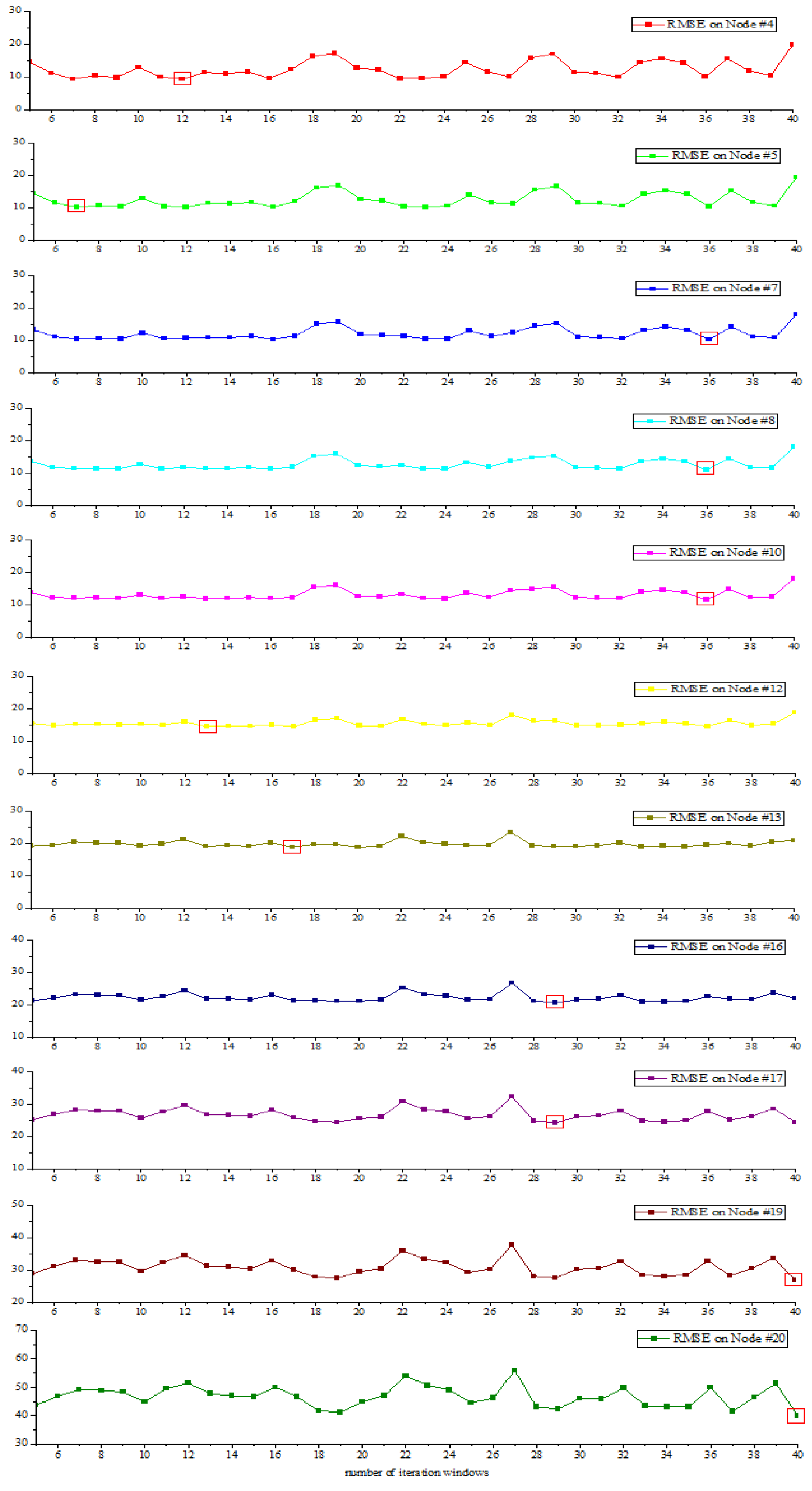
The data required for the entire model training are in the root node, so we use the data of the root node as the training set to train the global model. Different leaf nodes are used as different validation subsets to determine the parameters and validation errors of the global model. From Figure 4, we can see that the root node is node 0, and the leaf nodes are nodes 4, 5, 7, 8, 10, 12, 13, 16, 17, 19, and 20. Each node in the graph has its own dataset, and the number of iteration windows for the BLS is chosen from {5, 6,…, 40}. We use the validation set to tune the parameters of the network and choose the global model with the smallest RMSE at the root node. For node #4, we use the dataset of node #0 as the training set to train the BLS model. The data of node #4 are used as the validation set to adjust various parameters of the BLS model. Similarly, for nodes #5, #7, #8, #10, #12, #13, #16, #17, #19, and #20, we use the same method to verify. The training results of the global model are shown in Figure 6. The abscissa in the figure represents the number of iteration windows, and the ordinate represents the RMSE. We can see from the figure that different numbers of windows lead to different training results. Taking node #4 as an example, the optimal number of windows is 12. It can be seen that the optimal number of windows for the remaining 10 leaves are 7, 36, 36, 36, 13, 17, 29, 29, 40, and 40, respectively.

3.4.2. Local Model

In a CART decision tree, each internal node has its own data sample. On the internal nodes, the data of each internal node are used as the training set, and the data of the child nodes of the root node are used as the validation set. The training process is shown in Figure 7. Different sub-nodes are used as different validation subsets to determine the parameters and validation errors of the local model, respectively. Taking internal node #3 as an example, we regard this node as the root node, then nodes #4 and #5 are its child nodes. The data of node #3 consist of the training set, and we use the datasets of #4 and #5 to verify the parameters of the model, respectively. It can be seen that the optimal numbers of windows are 23 and 37, respectively.
On each terminal node of the decision tree, the dataset on the terminal node is divided into a training set and a validation set. The predictive model is trained using its own training dataset. The validation set is used to verify the error of the model, determine the final parameters of the model, and obtain a local BLS model.

3.5. Analysis of Experimental Results

This subsection presents the results of the experiments. We compare the global model RF and V-SVR models, as well as seasonality-based BLS. Table 2 presents the test errors of these models. Table 3 presents the test results of other index parameters of these models.
From the following table, we can see that the CART–BLS has the smallest RMSE on nodes #5, #7, #8, #10, #13, #16, and #17. Therefore, the accuracy of the model is highest on these nodes. On the whole, the RF model is better than the V-SVR model. Of course, on nodes #4, #19, and #20, the RF model predicts better than the rest. From looking at the dataset data, we know that PM2.5 is seasonal. Therefore, we do a local seasonal model test. On nodes #5, #8, and #10 the effect is basically the same as the model we used. Overall, the CART–BLS has a good prediction effect. In order to further verify the effectiveness of the model, we added other indicators. Table 4 presents the mean absolute error (MAE), mean absolute percentage error (MAPE), and correlation coefficient(R2) of different models on the testing set. The MAE, MAPE, and R2 are calculated by
M A E = 1 l i = 1 l | y i y ^ i | ,
M A P E = 1 l i = 1 l | y i y ^ i y i | , R 2 = 1 i ( y ^ i y i ) 2 i ( y ¯ i y i ) 2
As can be seen in Table 4, the MAE, MAPE, and R2 of the CART–BLS are lower. Compared with the other three models, we find that this model performs better.
According to the newly revised Ambient Air Quality Standard (GB3095-2012), combined with the air pollution data collected by us, the concentration range of PM2.5 and the ambient air quality level are determined. As shown in Table 5.
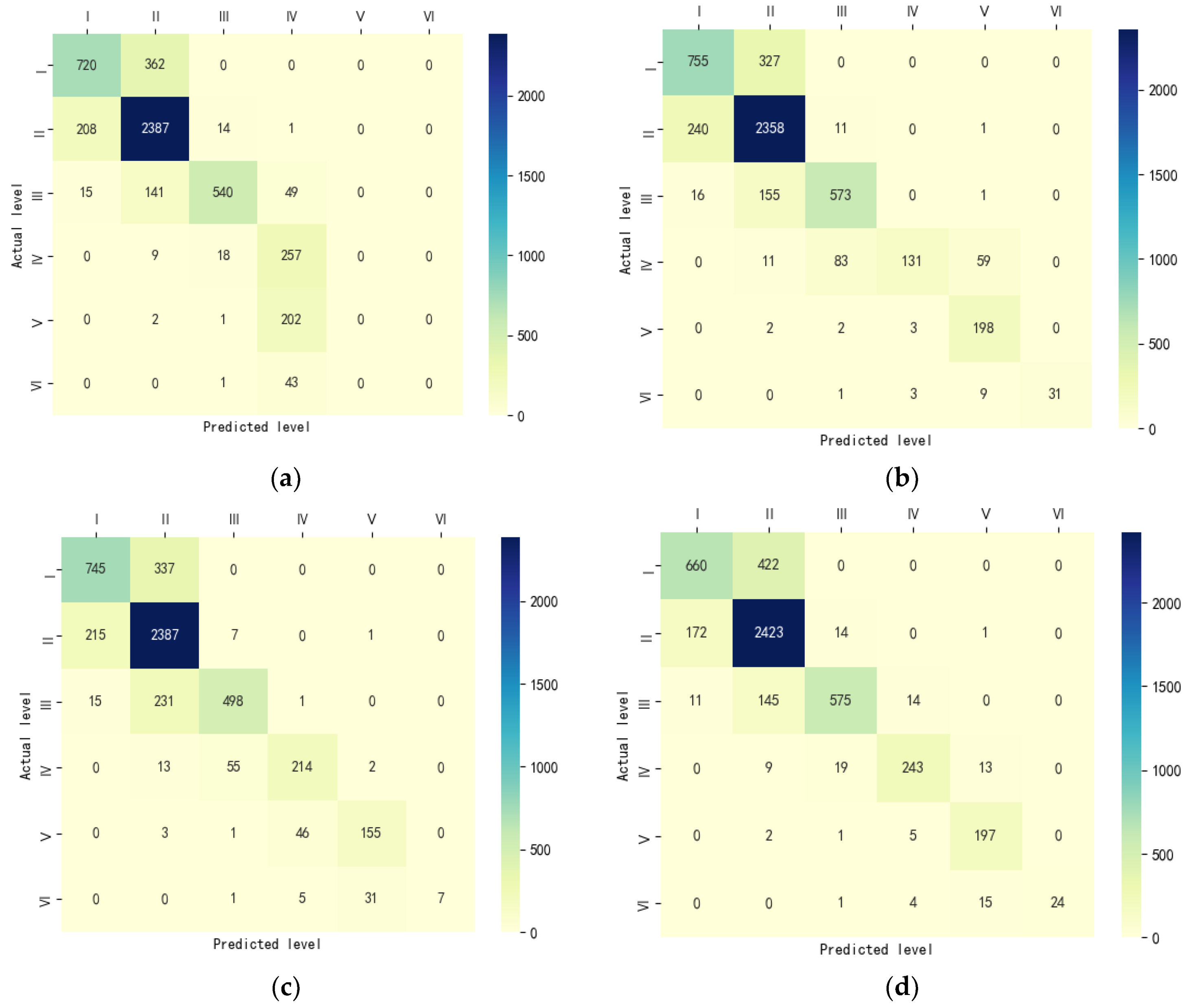
As shown in Table 5 above, the concentration of PM2.5 is divided into six levels. They are excellent (I), good (II), mild pollution (III), moderate pollution (IV), severe pollution (V), and severe pollution (VI). We conducted experiments on the test set, which tested the actual ranks corresponding to the PM2.5 concentrations of several models. The test results are shown in Figure 8, from which we can easily judge the distribution of the number of correct estimates, overestimates, and underestimates. Compared with overestimation, underestimation is more harmful to people’s health. In the first row of Figure (d) below, we illustrate the information in the figure. The first row shows that there are 1082 samples with actual grade I, 660 of which are correctly predicted, and 442 of which are overestimated as grade II. Figure 8 shows that the CART–BLS model has the most correct predicted samples as well as the smallest underestimation samples.

4. Conclusions

The complexity of PM2.5 data leads to an increased difficulty for the model to predict its accuracy. In view of the great potential of local models in improving prediction accuracy, the CART–BLS model is proposed. The model divides the training set into subsets using a CART decision tree and trains the BLS with its own training samples on each node of the division. Then, according to the prediction accuracy of each child node data sample, the validity of its model is judged.
Regarding the evaluated experimental results, the following conclusions can be drawn:
(1) We can conclude based on the BLS structure diagram in Figure 1 that the depth of the model simplified by the BLS network is used in this paper, and the complexity of the whole model is reduced by increasing the width of the network.
(2) According to the results of the relevant parameters in Table 2 and Table 4, it can be concluded that the CART–BLS model has a better prediction effect than the RF and V-SVR models.
(3) According to the results of the relevant parameters in Table 2 and Table 4, it can be concluded that the CART–BLS model has better results compared with the seasonal BLS model.

Author Contributions

Conceptualization, L.W., Y.W., and J.C.; methodology, L.W.; software, L.W. and Y.W.; validation, Y.W.; formal analysis, Y.W.; investigation, L.W. and Y.W.; resources, L.W.; data curation, L.W.; writing—original draft preparation, L.W.; writing—review and editing, L.W. and Y.W.; supervision, L.W.; project administration, L.W., J.C., and X.S.; funding acquisition, Y.W. All authors have read and agreed to the published version of the manuscript.

Funding

This research received no external funding.

Institutional Review Board Statement

Not applicable.

Informed Consent Statement

Not applicable.

Data Availability Statement

The datasets of the current study are available from the corresponding author on reasonable request.

Conflicts of Interest

The authors declare no conflict of interest.

References

  1. Thomaidis, N.S.; Bakeas, E.B.; Siskos, P.A. Characterization of lead, cadmium, arsenic and nickel in PM2.5 particles in the Athens atmosphere, Greece. Chemosphere 2003, 52, 959–966. [Google Scholar] [CrossRef]
  2. Zhou, Q.P.; Jiang, H.Y.; Wang, J.Z.; Zhou, J.L. A hybrid model for PM2.5 forecasting based on ensemble empirical mode decomposition and a general regression neural network. Sci. Total Environ. 2014, 496, 264–274. [Google Scholar] [CrossRef] [PubMed]
  3. Maftei, C.; Muntean, R.; Poinareanu, I. The Impact of Air Pollution on Pulmonary Diseases: A Case Study from Brasov County, Romania. Atmosphere 2022, 13, 902. [Google Scholar] [CrossRef]
  4. Byun, D.; Schere, K.L. Review of the Governing Equations, Computational Algorithms, and Other Components of the Models-3 Community Multiscale Air Quality (CMAQ) Modeling System. Appl. Mech. Rev. 2006, 59, 51–77. [Google Scholar] [CrossRef]
  5. Pouyaei, A.; Choi, Y.; Jung, J.; Sadeghi, B.; Song, C.H. Concentration trajectory route of air pollution with an integrated Lagrangian model (C-TRAIL model v1. 0) derived from the community Multiscale Air quality model (CMAQ model v5. 2). Geosci. Model Dev. 2020, 13, 3489–3505. [Google Scholar] [CrossRef]
  6. Lee, M.; Brauer, M.; Wong, P. Land use regression modelling of air pollution in high density high rise cities: A case study in Hong Kong. Sci. Total Environ. 2017, 592, 306. [Google Scholar] [CrossRef] [Green Version]
  7. Zafra, C.; Ángel, Y.; Torres, E. ARIMA analysis of the effect of land surface coverage on PM10 concentrationsin a high-altitude megacity. Atmos. Pollut. Res. 2017, 8, 1–12. [Google Scholar] [CrossRef]
  8. Lira, T.S.; Barrozo, M.A.S.; Assis, A.J. Air quality prediction in Uberlndia, Brazil, using linear models and neural networks. Elsevier 2007, 24, 51–56. [Google Scholar]
  9. Zhai, L.; Sang, H.; Zhang, J. Estimating the spatial distribution of PM2.5 concentration by integrating geographic data and field measurements. ISPRS Int. Arch. Photogramm. Remote Sens. Spat. Inf. Sci. 2015, XL-7/W4, 209–213. [Google Scholar] [CrossRef] [Green Version]
  10. Wang, Z.; Chen, J.; Zhou, C.; Wang, S.; Li, M. The Impacts of Urban Form on PM2.5 Concentrations: A Regional Analysis of Cities in China from 2000 to 2015. Atmosphere 2022, 13, 963. [Google Scholar] [CrossRef]
  11. Dong, Y.; Hui, W.; Lin, Z. An improved model for PM2.5 inference based on support vector machine. In Proceedings of the IEEE/ACIS International Conference on Software Engineering, Shanghai, China, 30 May–1 June 2016. [Google Scholar]
  12. Mogoll´on-Sotelo, C.; Casallas, A.; Vidal, S.; Celis, N.; Ferro, C.; Belalcazar, L.C. A support vector machine model to forecast ground-level PM2.5 in a highly populated city with a complex terrain. Air Qual. Atmos. Health 2021, 13, 399–409. [Google Scholar] [CrossRef]
  13. Zhu, W.; Wang, J.; Zhang, W.; Sun, D. Short-term effects of air pollution on lower respiratory diseases and forecasting by the group method of data handling. Atmos. Environ. 2012, 51, 29–38. [Google Scholar] [CrossRef]
  14. Jan, K.D.; Rasa, Z.; Mario, G. Modeling PM2.5 Urban Pollution Using Machine Learning and Selected Meteorological Parameters. J. Electr. Comput. Eng. 2017, 2017, 1–14. [Google Scholar]
  15. Cobourn, W.G. An enhanced PM2.5 air quality forecast model based on nonlinear regression and back-trajectory concentrations. Atmos. Environ. 2010, 44, 3015–3023. [Google Scholar] [CrossRef]
  16. Zhang, P.; Zhang, T.; He, L. Study on prediction and spatial variation of PM2.5 pollution by using improved BP artificial neural network model of computer technology and GIS. Comput. Model. New Technol. 2014, 18, 107–115. [Google Scholar]
  17. Linbo, L.; Lilong, L.; Junyu, L. Prediction of PM2.5 Mass Concentration Using GA-BP Neural Network Combined with Water Vapor Factor. J. Guilin Univ. Technol. 2019, 039, 420–426. [Google Scholar]
  18. Chen, L.; Pai, T.Y. Comparisons of GM(1,1), and BPNN for predicting hourly particulate matter in Dali area of Taichung City, Taiwan. Atmos. Pollut. Res. 2015, 6, 572–580. [Google Scholar] [CrossRef] [Green Version]
  19. Chen, C.; Liu, Z. Broad Learning System: An Effective and Efficient Incremental Learning System Without the Need for Deep Architecture. IEEE Trans. Neural Netw. Learn. Syst. 2018, 29, 10–24. [Google Scholar] [CrossRef]
  20. E, C.R.; Yuan, C.; Sun, Y.L.; Liu, Z.L.; Chen, L. Research progress of broad learning systems. Comput. Appl. Res. 2021, 38, 2258–2267. [Google Scholar]
  21. Tang, J.; Deng, C.; Huang, G.B. Extreme learning machine for multilayer perceptron. IEEE Trans. Neural Netw. Learn. Syst. 2016, 27, 809–821. [Google Scholar] [CrossRef]
  22. Chen, M.; Xu, Z.; Weinberger, K. Marginalized Denoising Autoencoders for Domain Adaptation. Comput. Sci. 2012, 1206, 1627–1634. [Google Scholar]
  23. Gong, M.; Liu, J.; Li, H.; Cai, Q.; Su, L. A multiobjective sparse feature learning model for deep neural networks. IEEE Trans. Neural Netw. Learn. Syst. 2015, 26, 3263–3277. [Google Scholar] [CrossRef]
  24. Shuang, F.; Chen, C. Transactions on Fuzzy Systems 1 A Fuzzy Restricted Boltzmann Machine: Novel Learning Algorithms Based on Crisp Possibilistic Mean Value of Fuzzy Numbers. IEEE Trans. Fuzzy Syst. 2016, 99, 1063–6706. [Google Scholar]
  25. Chen, C.L.P.; Zhang, C.Y.; Chen, L.; Gan, M. Fuzzy restricted Boltzmann machine for the enhancement of deep learning. IEEE Trans. Fuzzy Syst. 2015, 23, 2163–2173. [Google Scholar] [CrossRef]
  26. Yu, Z.; Li, L.; Liu, J.; Han, G. Hybrid adaptive classifier ensemble. IEEE Trans. Cybern. 2015, 45, 177–190. [Google Scholar]
  27. He, J.J.; Gong, S.L.; Yu, Y.; Yu, L.J.; Wu, L.; Mao, H.J. Air pollution characteristics and their relation to meteorological conditions during 2014–2015 in major Chinese cities. Environ. Pollut. 2017, 223, 484–496. [Google Scholar] [CrossRef] [PubMed]
  28. Mckendry, I.G. Evaluation of artificial neural networks for fine particulate pollution ([PM10] and [PM2.5]) forecasting. J. Air Waste Manag. Assoc. 2002, 52, 1096. [Google Scholar] [CrossRef] [PubMed] [Green Version]
  29. Yeo, I.; Choi, Y.; Lops, Y. Efficient PM2.5 forecasting using geographical correlation based on integrated deep learning algorithms. Neural Comput. Appl. 2021, 33, 15073–15089. [Google Scholar] [CrossRef]
  30. Li, S.; Xie, G.; Ren, J. Urban PM2.5 Concentration Prediction via Attention Based CNN–LSTM. Appl. Sci. 2020, 10, 1953. [Google Scholar] [CrossRef] [Green Version]
  31. Dai, H.; Huang, G.; Wang, J.; Zeng, H.; Zhou, F. Prediction of Air Pollutant Concentration Based on One-Dimensional Multi-Scale CNN-LSTM Considering Spatial-Temporal Characteristics: A Case Study of Xi’an, China. Atmosphere 2021, 12, 1626. [Google Scholar] [CrossRef]
  32. Huang, C.J.; Kuo, P.H. A Deep CNN-LSTM Model for Particulate Matter (PM2.5) Forecasting in Smart Cities. Sensors 2018, 18, 2220. [Google Scholar] [CrossRef] [Green Version]
  33. Celis, N.; Casallas, A.; Lopez-Barrera, E.; Martinez, H.; Peña, C.A.; Arenas, R.; Ferro, C. Design of an early alert system for PM2.5 through a stochastic method and machine learning models. Environ. Sci. Policy 2022, 127, 241–252. [Google Scholar] [CrossRef]
  34. Habibi, R.; Alesheikh, A.A.; Mohammadinia, A. An Assessment of Spatial Pattern Characterization of Air Pollution: A Case Study of CO and PM2.5 in Tehran, Iran. Int. J. Geo-Inf. 2017, 6, 270. [Google Scholar] [CrossRef] [Green Version]
  35. Jin, Y.J. Imputation adjustment method for missing data. Appl. Stat. Manag. 2001, 5, 47–53. [Google Scholar]
  36. Cheng, J.; Sun, J.; Yao, K.S.; Xu, M.; Cao, Y. A variable selection method based on mutual information and variance inflation factor. Spectrochim. Acta Part A Mol. Biomol. Spectrosc. 2022, 268, 1386–1425. [Google Scholar] [CrossRef]
  37. D, H.; Vu, K.M.; Muttaqi, A.P. A variance inflation factor and backward elimination based robust regression model for forecasting monthly electricity demand using climatic variables. Appl. Energy 2015, 140, 385–394. [Google Scholar]
  38. Thunis, P.; Pederzoli, A.; Pernigotti, D. Performance criteria to evaluate air quality modeling applications. Atmos. Environ. 2012, 59, 476–482. [Google Scholar] [CrossRef]
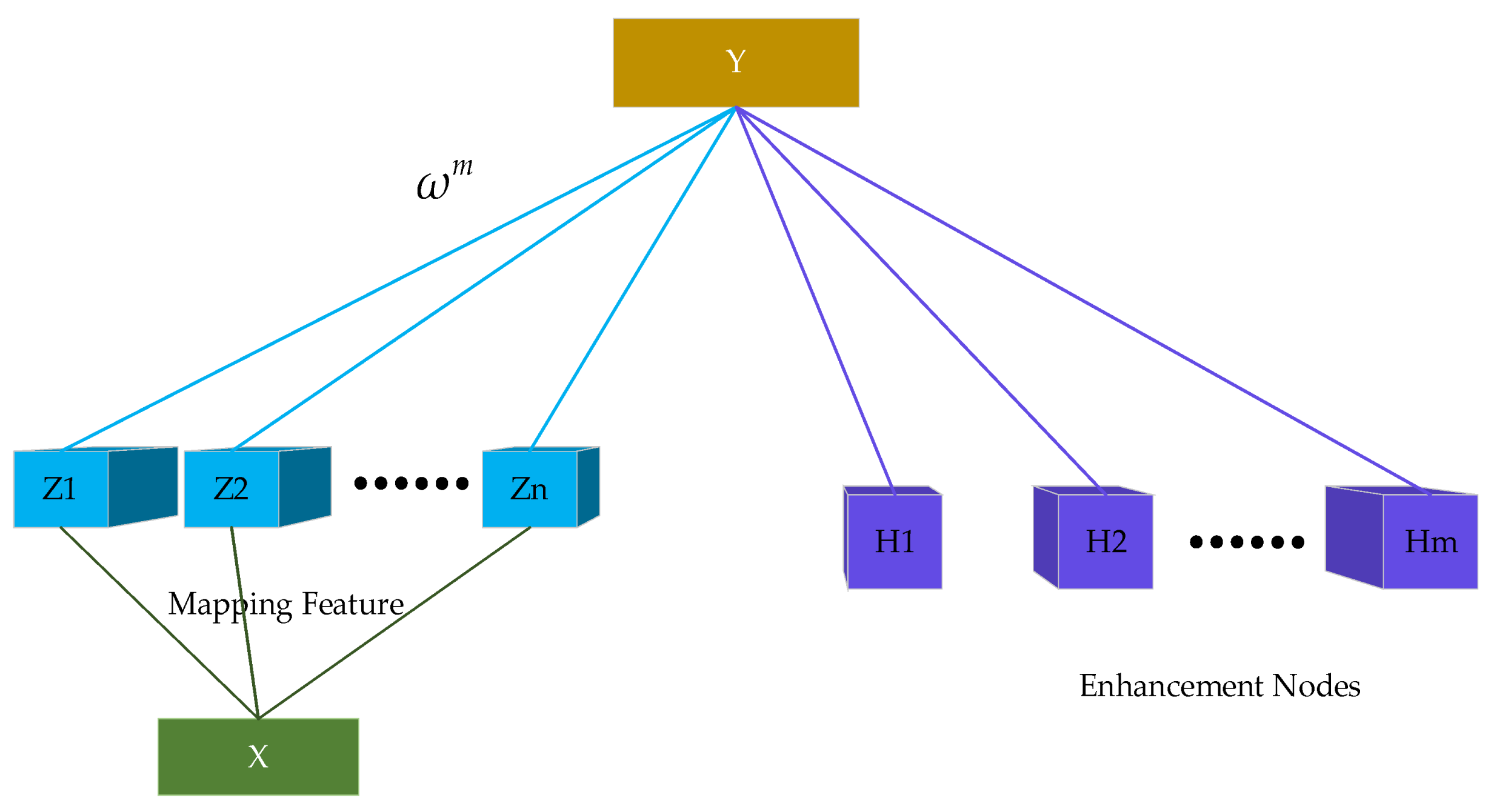
Figure 1. Network structure diagram of Broad Learning System.
Atmosphere 13 01674 g001
Figure 2. Location map of air monitoring stations.
Atmosphere 13 01674 g002
Figure 3. The importance ratio of each input vector.
Atmosphere 13 01674 g003
Figure 4. Training results of the CART. The # has no special meaning, and Node #0 represents node 0.
Atmosphere 13 01674 g004
Figure 5. Optimal parameter dendrogram for a BLS model. The # has no special meaning, and #0 represents node 0.
Atmosphere 13 01674 g005
Figure 6. Validation errors of the global models. All the red boxes in the figure represent the current nodes optimal RMSE values that we have marked.
Atmosphere 13 01674 g006
Figure 7. Validation errors of local models at node #3. All the red boxes in the figure represent the current nodes optimal RMSE values that we have marked.
Atmosphere 13 01674 g007
Figure 8. Statistical results of estimation levels for different models. (a) Statistical results of estimation levels for RF model; (b) statistical results of estimation levels for V-SVR model; (c) statistical results of estimation levels for Seasonal BLS model; (d) statistical results of estimation levels for CART–BLS model.
Atmosphere 13 01674 g008
Table 1. Correspondence of characteristic variables.
Input VectorFeature
X1, X2…, X11Temp, DPT, pressure, WD, WS, CO, NO2, O3, PM10, SO2, PM2.5
Table 2. VIF value of the input vector.
Input VectorX1X2X3X4X5X6X7X8X9X10X11
VIF3.671.1119,983.684.6910.167.614.299.942.949.47
Table 3. RMSE comparison of different models. The # has no special meaning, and #4 represents node 4.
ModelTesting RMSEs on the Leaf Nodes/μg·m−3
#4#5#7#8#10#12#13#16#17#19#20
RF2.922.331.581.590.905.965.574.966.999.8426.03
V-SVR3.442.361.621.540.935.565.564.777.029.8641.26
Seasonal BLS3.592.251.461.380.776.035.424.666.899.8940.27
CART–BLS3.542.251.451.380.776.035.404.646.869.8741.24
Table 4. Comparison of MAE, MAPE, and R2 of different models.
ModelTesting MAE/μg·m−3Testing MAPE/%R2
RF0.1706.2010.8146
V-SVR0.1668.3490.8419
Seasonal BLS0.1297.4510.8517
CART–BLS0.0684.4810.9362
Table 5. The ambient air quality levels and the corresponding concentration ranges.
PM2.5 Concentrations/μg·m−3[0,35](35,75](75,115](115,150](150,250](250, +∞)
LevelIIIIIIIVVVI
Publisher’s Note: MDPI stays neutral with regard to jurisdictional claims in published maps and institutional affiliations.