Cross-Examining Precipitation Products by Rain Gauge, Remote Sensing, and WRF Simulations over a South American Region across the Pacific Coast and Andes

Abstract

Precipitation estimate is important for earth science studies and applications, and it is one of the most difficult meteorological quantities to estimate accurately. For regions such as Peru, reliable gridded precipitation products are lacking due to complex terrains and large portions of remote lands that limit the accuracy of satellite precipitation estimation and in situ measurement density. This study evaluates and cross-examines two high-resolution satellite-based precipitation products, a global rain-gauge interpolated precipitation product, and a Weather Research and Forecast (WRF) model that simulated precipitation for a ten-year period from 2010 to 2019 in the Peruvian Andes region across the Pacific coast, Andes, and in the Amazon. The precipitation estimates examined in this study are the Integrated Multi-SatellitE Retrievals for GPM (IMERG), Multi-Source Weighted-Ensemble Precipitation (MSWEP), Global Precipitation Climatology Center product (GPCC), and a 3 km grid spacing WRF-based regional climate model (RCM) simulation. The evaluation and cross-examination were performed at sub-daily (6 h), daily, and monthly time scales, and at various spatial resolutions. The results show that the WRF simulation performs as well as, if not better than, GPM IMERG in the low precipitation and dry regions but becomes inaccurate in wet regions. GPM IMERG is more suitable for higher precipitation and wet regions, and MSWEP shows a systematic overestimation over the study area. It is therefore important to choose the most suitable precipitation product based on research needs and climate condition of the study for the challenging Peruvian Andes region.

1. Introduction

Precipitation is an important variable for atmospheric, hydrological, and environmental sciences. Therefore, estimating its values and quantifying its spatial–temporal variability are of paramount importance. Maintaining a dense network of rain gauge stations or weather radar (that are effective for Quantitative Precipitation Estimation or QPE) across a country can be very challenging for many parts of the world, especially for developing nations [1]. Peru is one of the South American countries that has additional challenges due to its complex terrain [2] making it difficult to establish a homogeneous rain gauge network [3] or a blockage-free weather radar network.

Satellite precipitation products are made available at high spatial and/or temporal resolutions by analyzing cloud-top temperature, cloud characteristics [4] or detecting microwave radiations from atmospheric hydrometeors, or a combination of both [5]. There are multiple global operational satellite precipitation products available such as the Tropical Rainfall Measuring Mission (TRMM) that operated from 1997 until 2015 [6], and its successor Integrated Multi-satellitE Retrievals for Global Precipitation Mission (GPM IMERG) from the National Aeronautics and Space Administration (NASA) [5,7,8]; the Climate Prediction Center (CPC) morphing technique (CMORPH) from the National Oceanic and Atmospheric Administration (NOAA) [9]; the Precipitation Estimation from Remotely Sensed Information Using Artificial Neural Networks (PERSIANN) from the University of Arizona and University of California Irvine [10,11]; and the Global Satellite Mapping of Precipitation Microwave-IR Combined Product (GSMaP-MVK) from the Earth Observation Research Center (EORC) of Japan Aerospace Exploration Agency (JAXA) [12]. However, a prior study [13] found that satellite- based precipitation products, such as PERSIANN, TRMM, CMORPH, and GSMaP, underestimated low precipitation and overestimated medium precipitation over the Peruvian Andes region. In a more recent study in 2019 [14], the most recent satellite precipitation products including GPM IMERG late run and final run, CMORPH, and GSMaP all overestimated the annual precipitation amount in the lower and higher elevation over the Peruvian Andes region.

The Global Precipitation Climatology Center (GPCC) climatology dataset is developed from 75,152 rain gauge stations over the world that partially covers the Peruvian Andes area, mostly along the Pacific Coast [15,16,17]. The GPCC precipitation product is interpolated from the global rain gauge network, and the sources of the data error are mainly the weather effects on rain gauge and gauge network density [16]. For complex terrain, a study evaluated GPCC among multiple precipitation products over the Qinling Mountains in China and found that the GPCC is reasonably good but less accurate compared to a local Chinese precipitation product called ITPCAS [18]. The performance of GPCC data along the Peruvian Andes has not been conducted yet. The Servicio Nacional de Meteorología e Hidrología del Perú (SENAMHI, the National Meteorological and Hydrological Service of Peru, https://www.gob.pe/senamhi, accessed on 4 May 2021) initiated a project called Peruvian Interpolated data of SENAMHI’s Climatological and Hydrological Observations (PISCOp V2.1) [19], which interpolated the Peruvian rain gauge network and the Climate Hazard Group Infrared Precipitation with Stations (CHIRPS) precipitation product [20]. However, due to the lack of rain gauge coverage in the Amazon rainforest, the PISCOp product was found to be less accurate in the Peruvian Amazon [19].

The Multi-Source Weighted-Ensemble Precipitation (MSWEP) is a global precipitation product that utilizes gauge interpolated precipitation products (WorldClim, and GPCC), satellite-based precipitation products (CMORPH, GSMaP, GridSat, and TRMM), and precipitation from reanalysis datasets (ERA-Interim and JRA-55) [21]. This product was developed to overcome the problems that satellite-based precipitation products have over mountainous regions. However, a study found that MSWEP overestimated over the Peruvian Andes region [14]. As the previous studies agreed that neither remote sensing technology, nor the rain gauge interpolation, nor the combination of both could produce accurate QPE over the Peruvian Andes region, this disadvantage is required to be further studied to provide insight for researchers if the inaccuracy of the global QPEs is homogeneous or heterogeneous over the region.

Another possible source of gridded precipitation estimate is numerical weather prediction (NWP) models. With advanced NWP models running at high spatial resolutions, one study [22] found that the Weather Research and Forecasting (WRF) model could produce more accurate gridded precipitation estimates than density-limited rain-gauge interpolated products in mountainous areas. Other studies have also explored this research direction since the challenge is substantially higher over complex terrain [23,24]. Moreover, with NWP models, there are potentials to forecast future precipitation to understand the impact of climate change [25]. A 2019 study indicated that the WRF dynamic downscaling performed better than the European Centre for Medium-Range Weather Forecasts Reanalysis (ERA-Interim) datasets over the tropical Andes region during the dry season [26]. Would NWP model estimated precipitation be a reliable source of a precipitation product for the Peruvian Andes region? It is a research question yet to be answered.

As the challenges exist for gridded precipitation products in complex terrains, and the scientific communities in countries such as Peru, Chile, Columbia, and Bolivia have disadvantages relative to developed countries with more comprehensive observational networks, it is important to understand the strengths and weaknesses of different precipitation products in different regions, given that the literature has not found that one product significantly outperforms others. This study presents a performance evaluation of GPM IMERG, MSWEP, GPCC, and a WRF dynamic downscaling over a very complex terrain in the Peruvian Andes region at sub-daily, daily, and monthly time scales in a ten-year period from 2010 to 2019. It also provides validation of the application of a WRF model to a challenging region in South America. The rest of this paper is organized as follows. Section 2 describes the study area, the precipitation datasets, and the statistical methods used in this study. Section 3 describes the findings of the analysis. Section 4 gives a discussion of some findings, and Section 5 concludes and summarizes this study and proposes future studies.

2. Materials and Methods

2.1. Study Area

This study was conducted in a South American region from the northwest corner at 80.0 W 5.0 S to the southeast corner at 63.5 W 24.5 S (Figure 1). This region consists of the majority of Peru, Bolivia, and a portion of Brazil, Chile, and Argentina. From the west coast facing the Pacific Ocean, to the Andean plateau, and then to the Amazon rainforest. This region has 12 out of total 30 different climate zones according to the Köppen–Geiger-Pohl climate classification (Figure 1) [27]. The 1 km current climate classification data were obtained from Nature Scientific Data [28]. The global climate classification map was then clipped within the study area and is presented in Figure 1. This region covers large climatical variations and precipitation diversities, which are driven by the interactions between synoptic-scale atmospheric current, orography of the Andes, the El Nino, and the cold Humboldt Current System (HCS) [29,30]. The average annual precipitation of the region ranges from less than 150 mm in the tropical desert climate to more than 3500 mm in the tropical rainforest climate [31].

2.2. Precipitation Products

The basic information and the average annual statistics of all precipitation products are listed in

Table 1. List of precipitation products analyzed in this study and their averaged annual precipitation statistics from 2010 to 2019.

	Resolutions		Annual Averaged Statistics from 2010 to 2019 (mm)
	Spatial	Temporal	Min	Median	Mean	Max	SD	25%	75%	Skewness	Kurtosis	CV
GPM IMERG	0.1°	0.5 h	5	1725	1483	5094	952	583	2212	0.00	1.93	0.64
MSWEP	0.1°	3 h	14	5097	4534	17,891	2259	2806	6645	0.11	2.40	0.50
WRF	3 km	1 h	0	2459	2352	43,462	1765	884	3367	2.39	24.41	0.75
GPCC	0.25°	1 month	6	2916	2671	12,044	1879	1131	3801	0.79	4.61	0.70

. A schematic flowchart of the series of analysis is displayed in Figure 2.

2.2.1. Rain Gauge

The 441 Peruvian daily rain gauges (Figure 1) records from 1981 to August 2018 were obtained from the National Service of Meteorology and Hydrology of Peru (SENAMHI, ftp://@ftp.senamhi.gob.pe/, accessed on 8 August 2021). The majority of the gauges data were collected manually; however, due to the inconsistency in the gauge observers that results in a change of data collecting method and precipitation truncation issues, the rain gauge data quality and continuity are considered as problematic [3]. The data had gone through a three-step quality control procedure to remove obvious inconsistent values, noisy extreme values, and manual removal of rounding patterns [19]. After eliminating the gauges located outside the study area, 393 daily rain gauge records were incorporated into the statistical analysis.

2.2.2. GPM IMERG

Building upon the TRMM project (1997), the NASA GPM mission was launched in 2014 and generates the quasi-global precipitation products, IMERG, at 0.1 arc-degree spatial resolution and 30 min temporal resolution [7,32,33,34]. In this study, the 30 min GPM IMERG final run data were downloaded from NASA GES DISC data archive (https://disc.gsfc.nasa.gov/, accessed on 4 May 2021 from 1 January 2010 to 31 December 2019, which was a rain gauge calibrated (RMSE minimization) precipitation product that was believed to be the most accurate and reliable in the GPM mission [8]. The data were then aggregated to 6 hourly rainfall rates (mm/h) using arithmetic mean, daily accumulated rainfall amount, and monthly accumulated rainfall amount for analysis. For the monthly analysis, the GPM IMERG data were further aggregated to 0.25 arc-degree using the median value to match the spatial resolution of GPCC precipitation product.

2.2.3. MSWEP

MSWEP V2.8 is an ensembled precipitation product that takes advantage of the multiple satellite precipitation estimates and daily rain gauge data. The MSWEP precipitation product provides seamless global precipitation values at 0.1 arc-degree spatial resolution and 3 h temporal resolution. The MSWEP data from 2010 to 2019 were obtained from Google shared drive (GoogleDrive:/MSWEP_V280/3hour/, accessed on 5 July 2021). Many studies have proven that MSWEP provides superior performance on accuracy of precipitation amount and drought detection in Iran, China, India, etc., and is a reliable dataset for climatological and hydrological studies [4,35,36,37]; however, its accuracy in the Peruvian region is questionable [14]. The data were aggregated to 6 hourly rainfall rate (mm/h) using arithmetic mean and daily accumulated rainfall amount for analysis.

2.2.4. GPCC Monthly Precipitation

Furthermore, 0.25 arc degree GPCC global monthly precipitation product was released in 2020 and obtained from the Federal Ministry of Transport and Digital Infrastructure of Germany (https://opendata.dwd.de/climate_environment/GPCC/html/fulldata-monthly_v2020_doi_download.html, accessed on 10 October 20201) [15]. Due to the low temporal resolution, the GPCC precipitation data were only used as a product to examine for seasonal features, and the extreme events information was not captured. Studies [38,39,40] indicated that the GPCC precipitation was one of the best precipitation products for long-term climatological and hydrological studies in many regions of the world. The data were clipped into the size of the study area for further analysis.

2.2.5. WRF Simulation

The WRF model v4.2.1 [41] was driven by the hourly European Centre for Medium-Range Weather Forecasts Reanalysis v5 (ERA5) data [42]. Two one-way nested domains with 15 and 3 km horizontal grid spacings covering the entire South America and the study area, respectively, were used. Spectral nudging technique was adopted to maintain large-scale circulations in the 15 km domain. The simulation period covered ten years (2010–2019) with an extra three months as a spin-up period.

The model physics schemes used in the simulation included Thompson microphysics scheme [43], Yonsei University (YSU) boundary layer scheme [44] the Rapid Radiative Transfer Model (RRTMG) longwave and shortwave radiation scheme [45], unified Noah land surface model (Noah) [46,47], and revised MM5 Monin–Obukhov surface layer scheme [48]. The cumulus parameterization scheme, Tiedtke [49], was only used for 15 km domain. The simulated hourly precipitation rate had been derived from the WRF output at 3 km spatial resolution over the study area, and the data were further aggregated to 6 hourly precipitation rate (mm/h), daily accumulated precipitation (mm/day), as well as monthly accumulated precipitation (mm/month). The data were spatially aggregated to 0.1 arc-degree and 0.25 arc-degree using the median value to meet the spatial resolutions of GPM IMERG, MSWEP, and GPCC datasets.

2.3. Statistical Metrics

There were three main and commonly used statistic tests conducted in this study, which were correlation coefficient (CC), normalized bias, and root-mean squared error/root-mean squared difference (RMSE/RMSD) [50,51]. The metrics and their equations are listed in

Table 2. List of statistical metrics.

Statistic Metrics	Equation	Value Range	Perfect Value
Correlation coefficient (CC)	$CC=\frac{{{\displaystyle \sum }}_{n=1}^N\left(f_n-\overline{f}\right)\left(r_n-\overline{r}\right)}{\sqrt{{{\displaystyle \sum }}_{n=1}^N{\left(f_n-\overline{f}\right)}^2}\sqrt{{{\displaystyle \sum }}_{n=1}^N{\left(r_n-\overline{r}\right)}^2}}$	−1, 1	1
Normalized bias (NB)	$NB=\frac{1}{N}{\displaystyle {\displaystyle \sum }_{n=1}^N}\frac{f_n-r_n}{f_n+r_n}$	−1, 1	0
Root-mean-square error/difference (RMSE/RMSD)	$RMSE/RMSD=\sqrt{\frac{1}{N}{\displaystyle {\displaystyle \sum }_{n=1}^N}{\left(f_n-r_n\right)}^2}$	0, +∞	0
a Variables: n and N, sample index and a total number of samples; f represents the precipitation estimates; r represents the reference.

.

The correlation coefficient (CC) over a time series measures the strength of an estimate to capture the temporal pattern of the observation, ranging from −1 to 1. The normalized bias (NB, fraction) is a normalized measurement to quantify the error of the estimated precipitation as a fraction of the sum of observation and estimation, which has the range from −1 to 1. The root-mean squared error (RMSE, mm/h or mm) measures the distance between the estimates and the observation, ranging from 0 to positive infinity. For inter-comparison between different precipitation products, there is no “ground truth” to be the reference; thus, the same calculation as RMSE is performed to measure the difference between two precipitation products and is called the root-mean squared difference (RMSD, mm/h or mm).

Due to the different temporal resolution of precipitation estimates, the statistical analysis is divided into three sections (Figure 2). The rain gauge evaluation was at the daily level, including GPM IMERG, MSWEP, and WRF simulation. The cross-comparison was at the sub-daily level (6 h, storm-permitting) between GPM IMERG, MSWEP, and WRF simulation. The monthly Multiplicative Triple Colocation (MTC) analysis was at monthly level, including GPM IMERG, CPCC, and WRF simulation. The daily evaluation was divided into different climate zones and months to detect the spatial and seasonal variations. The cross-comparison analysis was divided into climate zone to test the spatial similarities between precipitation products, and the MTC analysis was divided into annual precipitation intervals to detect the impact of precipitation intensity to precipitation products.

2.4. Triple Colocation (TC) Method

When the “ground truth” is not available, which commonly happens in ocean and mountainous areas, the TC method could be applied to estimate the CC and RMSE between three independent and unrelated datasets that measure the same variable. The TC method has three assumptions to comply for analysis: (a) the three precipitation products are independent; (b) the errors of the independent precipitation products are also independent or are unrelated; (c) the expected value of error is 0. The independence of the three analyzed datasets was proven to be negatively correlated with the TC induced error [52,53,54]. Another principle of the TC method is that it treats all three independent datasets that are equally important, and no bias can be produced in between. The CC and RMSE are then derived by using a linear combination of three datasets and affine transformed error model [55]. For precipitation error estimation (RMSE), a multiplicative logarithm transformation (Multiplicative Triple Colocation, MTC) was proposed and proven to be a better approach [52,53,56,57]. The detailed mathematical derivation and explanation are listed in Appendix A. To meet the MTC assumption requirements, GPM IMERG V6 final, WRF simulation, and GPCC precipitation products were selected to conduct the MTC analysis. To compensate for the lower spatial and temporal resolution of GPCC precipitation, both GPM IMERG and WRF simulated precipitation data were aggregated to 0.25 arc-degree and monthly accumulated rainfall. The monthly analysis can only explore the seasonal differences and errors from the three precipitation products. MSWEP utilizes both GPM IMERG and GPCC datasets that violate the independence assumption of the MTC method; thus, it was not included in the MTC analysis.

3. Results

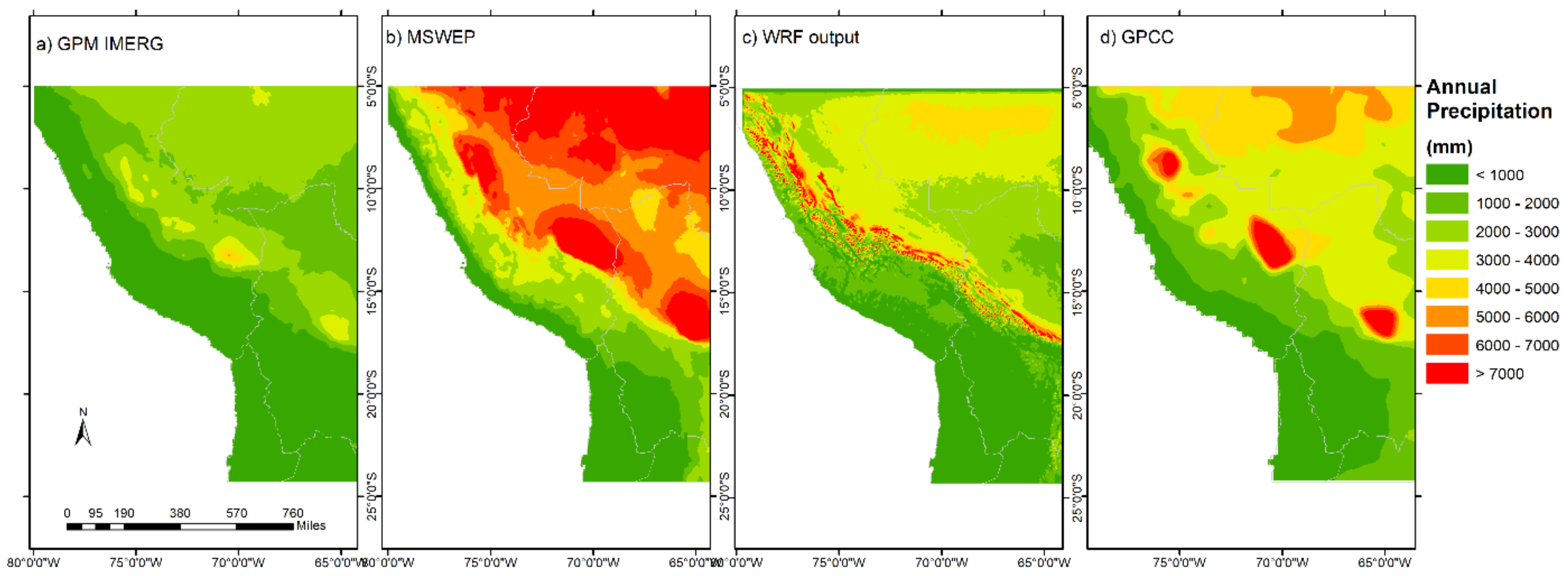
3.1. Annual Mean of Precipitation Products

The basic statistics and the maps of the average annual precipitation for all four precipitation products at their original spatial resolutions are listed in Table 1 and are shown in Figure 3. All four precipitation products showed similar spatial patterns of high and low rainfall areas, where the large precipitation rates were concentrated at the east slope (upwind) of the Andes and the Amazon rainforest and low precipitation areas concentrated between the west side of the Andes and the Pacific Ocean. The WRF simulation showed more scattered high volumes of precipitation along the east slope (upwind) of the Andes. The MSWEP appeared to have polygon-shaped precipitation clusters over the Amazon (upper right of the maps in Figure 3), while other products had a smoother precipitation band. However, the magnitudes of the average annual precipitation from the four products were different. The median of the 10-year average rainfall in the study for MSWEP (5097 mm) was almost twice as much as WRF simulation (2459 mm) and more than twice as much as GPM IMERG (1725 mm). The maximum precipitation value of MSWEP (17,891 mm) was more than three times the amount of the maximum value of GPM IMERG (5094 mm), and both precipitation products had the same spatial resolution at 0.1 arc-degree, which indicated a lack of consistency in precipitation amounts across the products in this study. GPCC had been considered as a highly accurate gauge-based precipitation product in previous studies [39,58], and had a similar annual mean precipitation (2671 mm) as the WRF simulation (2352 mm) from 2010 to 2019. A 1980s study that is commonly referenced by non-scientific media indicates that the annual rainfall in the Amazon Rainforest (right upper portion of the maps in Figure 2) ranges from 1500 to 3000 m [59], which was less than most of the annual precipitations from the products in this study except for GPM IMERG (2000–3000 mm). It was uncertain whether the difference between the 1980s and 2010s annual rainfall was caused by overestimation or climate change, which could be explored in a future study.

3.2. Daily Ground Observation Evaluations

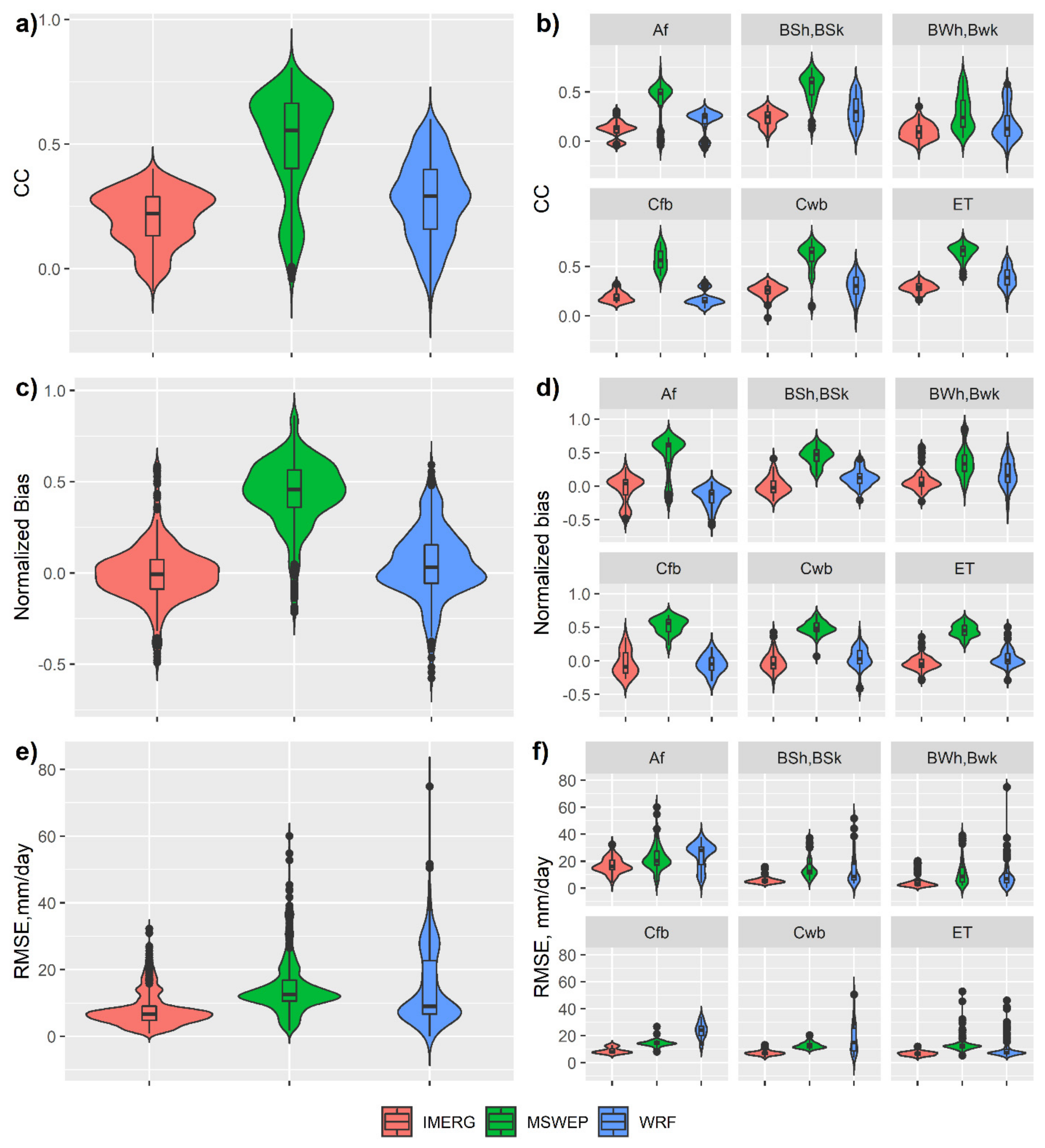
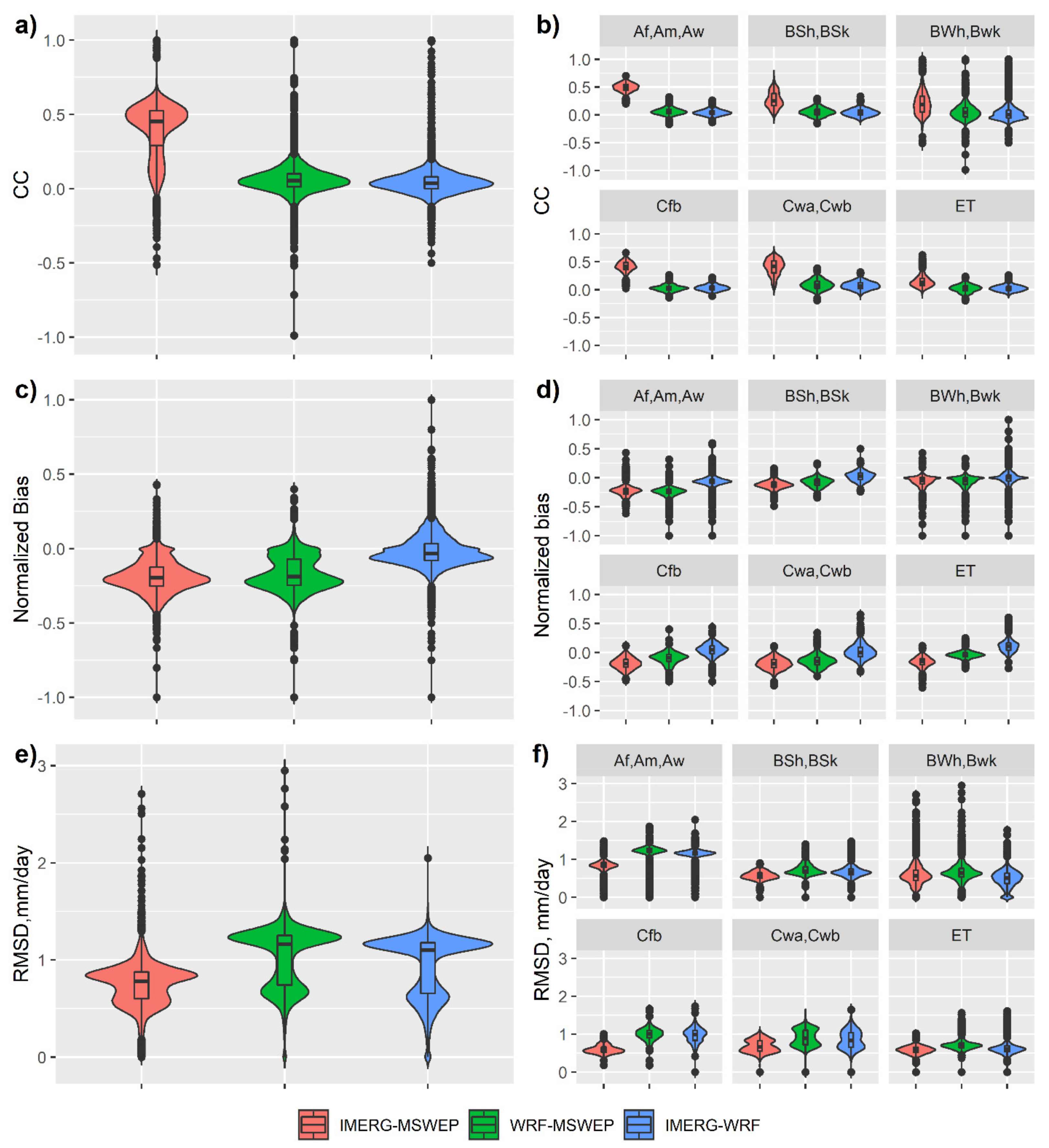
3.2.1. Daily Analysis over Different Climate Zones in Peru

By comparing the daily precipitation data from 401 rain gauges from January 2010 to July 2018, the analytical results are listed in

Table 3. The average statistic values of precipitation products comparing the Peruvian rain gauge data from 2010/01 to 2018/07.

		GPM IMERG	MSWP	WRF
CC	Min	−0.09	0.03	−0.15
	Median	0.24	0.59	0.30
	Mean	0.22	0.54	0.30
	Max	0.40	0.81	0.60
NB (%)	Min	−29.37	−9.90	−35.04
	Median	−0.72	46.94	3.67
	Mean	0.28	45.37	6.92
	Max	57.88	84.69	59.29
RMSE (mm)	Min	0.96	1.70	0.10
	Median	6.37	12.35	8.50
	Mean	7.40	14.24	14.20
	Max	32.27	60.05	74.89

, and the spatial distribution is shown in Figure 4. GPCC was not included in the daily analysis due to its low temporal resolution.

In the Peruvian region, the MSWEP precipitation product had the highest temporal correlations (mean 0.54, max 0.81) with the rain gauge data; however, this product had a systematic overestimation, which is consistent with findings from another study [14], where the mean of NB was 46.94%, which was much higher than the GPM IMERG (0.28%) and WRF simulation (6.92%). In Figure 4, the map showed a wide range of overestimations by MSWEP of over 25% NB values across the Peruvian region. Consequentially, the RMSE was the highest for MSWEP (mean 14.24 mm, max 60.05 mm) among all three precipitation products. Both GPM IMERG and WRF simulations have lower CC values (0.22 and 0.30 respectively), and most of the low to negative CC values were concentrated along the coast for both products. GPM IMERG has more low CC sites and slightly underestimated the precipitation with the median of the NB at −0.72%, yet it had the lowest RMSE (mean 7.40 mm, median 6.37 mm) compared to WRF and MSWEP. From Figure 4, most of the negative biases of IMERG were located along the east slope (upwind) of the Andes, and the positive bias was located at the west slope (downwind) of the Andes. On the daily scale, GPM IMERG had the most accurate precipitation quantities estimate but did not capture the temporal variations well. The WRF simulation was relatively closer to the optimal NB value but had a high RMSE (mean 14.20 mm). The median of RMSE for the WRF simulation was 8.50 mm, which means that there were extreme RMSE values that skewed the sample distribution and drove up the mean value. In Figure 4, most of the high RMSE values for the WRF simulation were close to the equator.

As the precipitation products performed variously across different geographic locations and climate zones, Figure 5 displays insight into their statistical scores in six major climate groups identified by Köppen–Geiger–Pohl classification. The systematic positive bias from MSWEP was consistent with the findings from Figure 4, where the tropical rainforest climate (Af) area had a higher positive bias than other climate zones. Generally, the WRF simulation had slightly higher CC than GPM IMERG in all climate zones, except for the marine west coast climate (Cfb) along the east slope (upwind) of the Andes.

GPM IMERG had negative biases in almost all climate zones except for the tropical rainforest. WRF simulation had positive biases in desert and grassland areas (BSh, BSk, BWh, BWk) but negative biases in tropical rainforest and marine west coast climates (Af and Cfb), which means that the WRF simulation slightly underestimated in the higher precipitation areas and overestimated in the dryer areas. In wetter climates (Af and Cfb), the WRF simulation had the highest RMSEs. Both GPM IMERG and WRF simulations had close to zero bias and lower RMSEs in the cold climate (Cwb and ET). By giving a ranking score of 1 for the highest score of the statistic metric and 3 for the lowest to GPM IMERG, MSWEP, and WRF, the combined scores indicated that GPM IMERG has better performances in tropical rainforest climates and Marine west coast climates, and the WRF simulation had better performances in dryer climates such as desert, grassland, and tundra climates (

Table 4. Performance ranking for GPM IMERG, MSWEP, and WRF in major climate zones in Peru, where the best scores were highlighted in green.

	CC	Bias	RMSE	Sum	CC	Bias	RMSE	Sum
Af: Tropical Rainforest					Cfb: Marine West Coast
IMERG	3	1	1	5	2	2	1	5
MSWEP	1	3	2	6	1	3	2	6
WRF	2	2	3	7	3	1	3	7
BSh, BSk: mid-latitude desert and grassland					Cwb: cold humid subtropical climate
IMERG	3	1	2	6	3	2	1	6
MSWEP	1	3	3	7	1	3	2	6
WRF	2	2	1	5	2	1	3	6
BWh, BWk: tropical and subtropical desert					ET: tundra climate
IMERG	3	1	2	6	3	2	1	6
MSWEP	1	3	3	7	1	3	3	7
WRF	2	2	1	5	2	1	2	5

).

3.2.2. Seasonal Statistical Results in Different Climate Zones

The monthly performance from 2010 to 2019 across different climate zones is displayed in a pivot table (

Table 5. Monthly average statistical results for 2010–2018 for precipitation products in six major climate zones in Peru, where red or blue indicated poor performance and green indicated closer to optimal performance.

CC		Jan	Feb	Mar	Apr	May	Jun	Jul	Aug	Sep	Oct	Nov	Dec
Af	IMERG	0.04	0.05	0.04	0.07	0.06	0.06	0.07	0.06	0.07	0.05	0.05	0.06
	MSWEP	0.33	0.33	0.32	0.37	0.34	0.32	0.32	0.32	0.35	0.34	0.33	0.32
	WRF	0.20	0.16	0.14	0.17	0.14	0.18	0.18	0.22	0.17	0.16	0.14	0.11
BSh, BSk	IMERG	0.12	0.08	0.09	0.11	0.05	0.04	0.05	0.03	0.07	0.04	0.04	0.05
	MSWEP	0.52	0.53	0.50	0.44	0.30	0.22	0.22	0.21	0.26	0.34	0.35	0.44
	WRF	0.23	0.16	0.18	0.21	0.13	0.17	0.16	0.14	0.12	0.12	0.14	0.11
BWh, BWk	IMERG	0.04	0.02	0.06	0.05	0.01	0.02	0.02	0.01	0.03	0.02	0.00	0.04
	MSWEP	0.29	0.33	0.30	0.20	0.16	0.16	0.16	0.12	0.11	0.15	0.13	0.23
	WRF	0.17	0.15	0.13	0.12	0.08	0.09	0.11	0.09	0.07	0.04	0.06	0.07
Cfb	IMERG	0.06	0.11	0.10	0.07	0.11	0.00	0.04	0.06	0.10	0.06	0.09	0.06
	MSWEP	0.49	0.48	0.52	0.52	0.53	0.40	0.37	0.39	0.45	0.47	0.52	0.48
	WRF	0.14	0.07	0.08	0.10	0.10	0.10	0.10	0.10	0.08	0.07	0.09	0.06
Cwb	IMERG	0.07	0.07	0.09	0.08	0.06	0.02	0.04	0.03	0.07	0.06	0.04	0.03
	MSWEP	0.47	0.44	0.47	0.48	0.42	0.34	0.33	0.35	0.39	0.46	0.47	0.45
	WRF	0.16	0.11	0.13	0.17	0.17	0.20	0.21	0.24	0.14	0.11	0.12	0.08
ET	IMERG	0.08	0.07	0.09	0.12	0.04	0.04	0.04	0.03	0.07	0.05	0.01	0.07
	MSWEP	0.52	0.50	0.51	0.52	0.36	0.32	0.34	0.33	0.41	0.47	0.47	0.51
	WRF	0.24	0.17	0.22	0.24	0.18	0.26	0.27	0.24	0.23	0.22	0.22	0.11
Bias (%)		Jan	Feb	Mar	Apr	May	Jun	Jul	Aug	Sep	Oct	Nov	Dec
Af	IMERG	−2.42	−2.18	−1.48	−2.41	−1.83	−1.37	−1.63	−0.09	−0.57	−1.57	−0.58	−0.93
	MSWEP	1.44	3.35	3.42	3.49	3.48	2.92	2.79	3.01	3.36	3.32	3.64	3.42
	WRF	−2.59	−2.38	−2.97	−2.82	−2.65	−1.83	−1.42	−1.02	−1.23	−1.97	−1.69	−2.08
BSh, BSk	IMERG	−1.99	−1.83	−2.08	−1.58	−0.30	−0.11	−0.41	0.00	−0.39	−0.63	−0.36	−1.04
	MSWEP	3.60	3.68	4.31	3.37	2.29	0.76	0.43	0.84	1.48	1.62	1.53	1.93
	WRF	−0.35	−0.01	−0.85	−0.21	−0.02	−0.27	−0.33	0.18	1.12	0.00	0.59	0.80
BWh, Bwk	IMERG	−0.31	−0.50	−0.35	−0.07	−0.18	−0.22	−0.48	−0.35	−0.09	−0.24	−0.06	0.14
	MSWEP	2.34	2.63	2.49	1.49	1.86	1.09	0.63	0.36	1.08	0.86	0.83	1.08
	WRF	0.74	1.36	0.92	0.23	0.17	−0.24	−0.35	−0.02	0.85	0.44	0.76	1.54
Cfb	IMERG	−2.22	−2.05	−1.93	−1.48	−1.33	−0.97	−1.54	−0.01	−0.98	−0.66	−0.39	−0.85
	MSWEP	4.61	4.01	5.04	4.96	4.73	2.95	0.48	2.68	4.03	3.68	3.84	2.57
	WRF	−2.06	−1.29	−1.69	−2.03	−1.85	−1.05	−1.36	−0.26	−0.37	−1.57	−0.53	−1.09
Cwb	IMERG	−1.90	−1.95	−1.74	−1.57	−0.63	−0.23	−0.40	−0.18	−1.05	−0.82	−0.77	−1.47
	MSWEP	4.71	3.91	4.97	4.17	3.18	1.09	0.15	0.47	3.11	3.25	3.53	3.57
	WRF	−0.62	−0.45	−1.14	−1.03	−0.94	−0.47	−0.42	0.06	0.49	−0.25	−0.30	−0.49
ET	IMERG	−2.21	−1.95	−2.08	−2.11	−0.59	−0.35	−0.51	−0.38	−0.98	−1.18	−0.93	−1.89
	MSWEP	4.81	4.36	5.07	3.40	2.75	0.35	0.35	0.26	2.33	1.82	1.98	3.14
	WRF	−0.81	−0.76	−1.43	−1.08	−0.15	−0.26	−0.32	−0.17	0.67	−0.33	−0.25	−0.68
RMSE (mm)		Jan	Feb	Mar	Apr	May	Jun	Jul	Aug	Sep	Oct	Nov	Dec
Af	IMERG	4.96	5.60	6.44	4.59	4.01	3.18	2.32	2.84	3.21	3.71	4.90	4.62
	MSWEP	7.01	8.47	8.89	8.24	5.11	3.67	3.36	4.00	4.82	6.48	6.99	6.82
	WRF	7.08	7.88	8.74	6.45	5.71	4.48	3.20	3.68	5.23	5.53	7.22	7.31
BSh, BSk	IMERG	2.28	2.69	3.02	1.47	0.70	0.39	0.19	0.24	0.36	0.68	0.71	1.31
	MSWEP	5.53	8.13	6.41	3.15	1.53	0.48	0.43	0.43	0.91	1.71	1.52	2.74
	WRF	3.87	4.84	4.61	3.69	2.20	0.71	0.38	1.26	2.21	2.27	2.79	3.83
BWh, Bwk	IMERG	1.57	2.09	2.14	1.08	0.48	0.37	0.10	0.09	0.21	0.37	0.27	0.92
	MSWEP	4.18	6.05	4.29	2.59	1.33	0.94	0.44	0.37	1.05	1.14	1.37	2.43
	WRF	3.03	3.33	3.01	1.55	0.96	0.29	0.20	0.33	1.22	0.99	1.46	2.60
Cfb	IMERG	2.76	3.24	3.61	2.77	2.07	1.29	0.91	1.26	1.38	2.35	2.07	2.52
	MSWEP	5.30	5.92	6.96	4.69	3.21	1.42	1.14	1.74	2.59	4.13	3.87	4.56
	WRF	6.86	7.18	8.04	6.37	4.81	3.26	2.15	3.40	3.88	5.81	7.27	7.37
Cwb	IMERG	2.73	2.90	2.94	1.77	1.14	0.55	0.48	0.54	0.89	1.54	1.54	2.45
	MSWEP	4.98	5.77	5.44	3.24	1.75	0.66	0.54	0.79	1.57	3.06	2.93	4.34
	WRF	5.81	6.13	6.08	4.51	2.56	1.38	0.88	2.05	3.59	4.30	4.84	5.45
ET	IMERG	2.90	2.85	2.51	1.34	0.72	0.30	0.30	0.34	0.76	1.12	1.11	2.33
	MSWEP	5.73	7.56	5.50	2.66	1.29	0.44	0.55	0.51	1.26	1.96	2.01	4.38
	WRF	3.92	4.14	3.48	2.47	1.43	0.59	0.53	0.79	2.11	2.29	2.44	3.61

). The optimal statistical scores are all marked “green” in Table 5, while the lower scores are marked “red” for CC and RMSE. The highest 10% of positive bias is marked “red” and the highest 10% of negative bias is marked “blue”. For the tropical rainforest climate representing the high precipitation and high temperature climate, GPM IMERG had low CC in all months and moderate negative bias during the spring (Aug–Nov) in the southern hemisphere, which is the dry season in Peru. GPM IMERG had more negative biases during the later summer and fall (Jan–April) when the season is wetter. The highest RMSE for IMERG in the tropical rainforest climate was 6.44 mm in March, which is the last month of the Peruvian raining season. MSWEP had higher CC in a tropical rainforest climate compared to IMERG and WRF, where the transitions from fall to winter (Apr–May) and from winter to spring (Sep–Oct) were the highest periods. The RMSE of MSWEP at tropical rainforest reduced during the dry and cold season (Jun–Jul), and it has positive bias in all months. The WRF simulation had slightly higher CC than GPM IMERG in tropical rainforest throughout the years, but greater negative bias than IMERG during the rainy season and less negative bias during the dry season.

For the dry climates of mid-latitude desert/grassland (BSh, BSk) and tropical/subtropical desert (BWh, BWk), both GPM IMERG and WRF simulations had less than ±0.5% of bias in the majority of months. IMERG had slightly more accurate estimation than WRF in tropical/subtropical desert, and WRF had slightly more accurate precipitation estimation than IMERG in mid-latitude desert/grassland. All three precipitation products had less than 0.5 mm of error (RMSE) during the dry seasons in the dry climates, but the error tended to increase more for MSWEP in wet seasons compared to IMERG and WRF. MSWEP maintained higher CC in the mid-latitude desert/grassland climate, but the CC score was reduced in tropical/subtropical desert climates. These findings were not surprising, such that precipitation estimates perform the best for moderate rainfall but are not accurate temporally for the dry and wet extremes. The bias and error reduced during the dryer area and seasons for all precipitation products.

For the marine west coast climate and cold humid subtropical climate, which are located along the east slope (upwind) of the Andes at high altitude, IMERG and WRF had close to 0 CC values. GPM IMERG had about 2% negative bias during the raining season (Jan–Mar) for marine west coast and humid subtropical climate, which indicates that GPM IMERG performed worse on the east slope (upwind) of the Andes than the west slope (downwind) during the raining season. WRF simulation also had large negative bias during the raining season (Jan–Apr) for the marine west coast climate but had better performance in the cold humid subtropical climate. Consequentially, the RMSE was very large during the same months for the WRF simulation.

For the tundra climate, which is mostly located at the peak and ice cap regions of the Andes, both MSWEP and GPM IMERG had lower CC during the dry winter season compared to other months, but the MSWEP CC score ranged from 0.32 to 0.52 while IMERG generally had very poor CC that ranged from 0.01 to 0.12. WRF simulation had a more consistent CC value across the months and had close to an optimal bias (absolute bias < 1%) from May to November. MSWEP had a large positive bias, and IMERG had a large negative bias during the raining season (Jan–Apr) in tundra climate.

Based on the analysis, the precipitation products tended to have larger bias and error when precipitation increases during the raining season, and the temporal correlation reduced in the dry and wet extremes. Generally, precipitation products were more accurate in dryer climate during the dryer season, especially for the WRF simulation, and the findings from Section 3.2.1 are consistent with this section’s results.

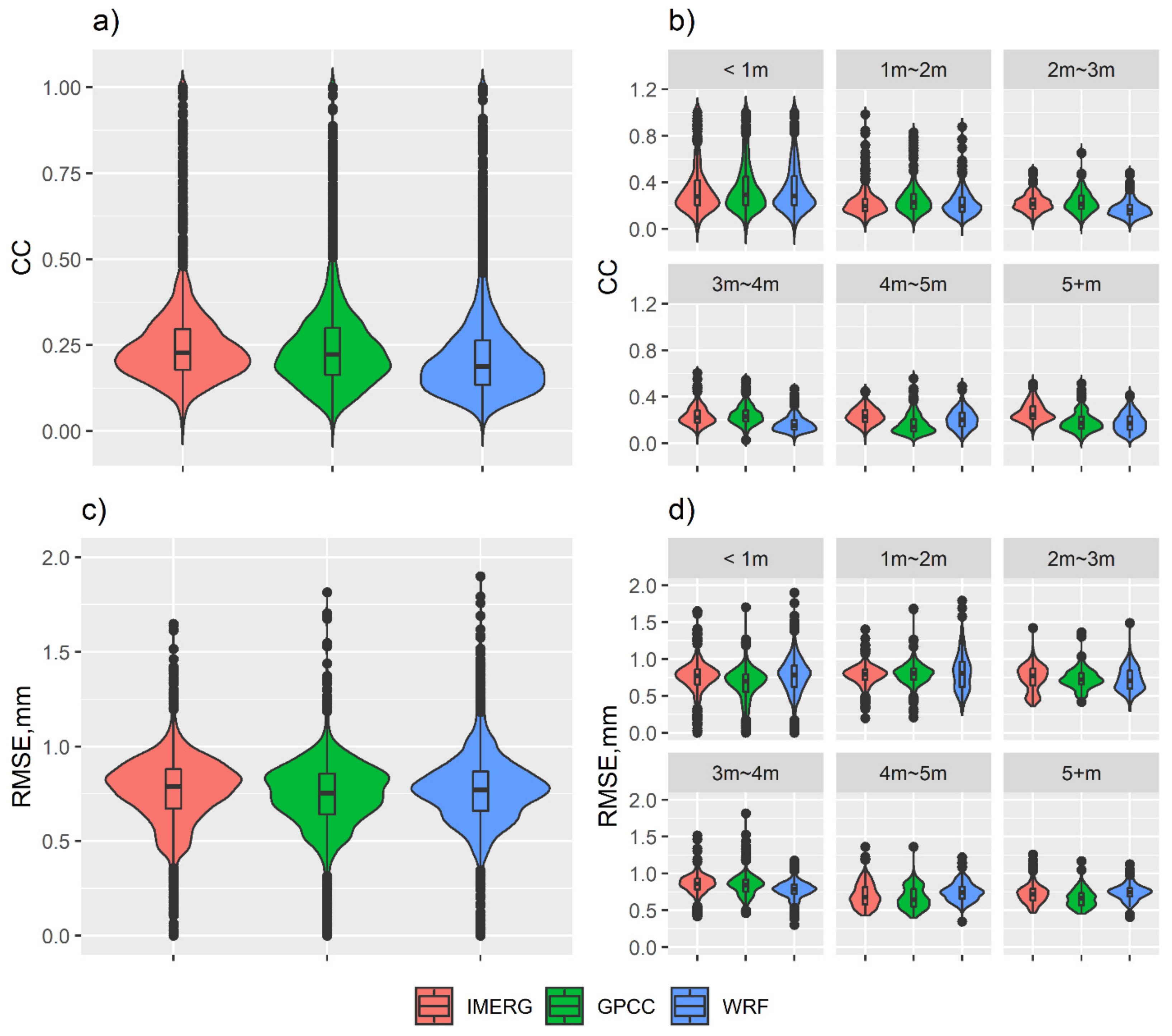
3.3. Statistical Cross-Examination at Sub-Daily Scale

MSWEP, GPM IMERG, and WRF simulation all have high temporal resolutions that allows one to observe short-term storms. From Section 3.2, the WRF simulation was more accurate at dryer regions, GPM IMERG was more accurate at wetter regions, and MSWEP was more capable to capture the temporal pattern rather than the precipitation intensity at daily scale. Since sub-daily precipitation data contains more climate dynamic and variability signals, we analyzed their sub-daily differences and similarities between each pair of products. Moreover, it is important to determine if the WRF dynamic downscaling can match satellite observations at high temporal resolution. The results are demonstrated in Figure 6 and Figure 7.

MSWEP product includes the GPM IMERG as one of the input datum [21]; therefore, both the correlation (CC) between IMERG and MSWEP was higher, and difference (RMSD) was lower; however, the tropical/subtropical desert climate had some pixels with lower CC value, which is demonstrated in Figure 6a with yellow to orange color in the desert area. The same results can be found consistently in six major climate zones, except for the tropical/subtropical desert climate (BWh, BWk) and tundra climate (ET), where the CC and RMSD between the WRF simulation and IMERG were comparably as low as the IMERG-MSWEP pair. The MSWEP had higher precipitation amounts in this study area based on the analysis from Section 3.1 and Section 3.2; thus, the IMERG-MSWEP and WRF-MSWEP pair had obvious negative bias across all climate zones except for the tropical/subtropical desert climate area, where the compared pairs showed that the bias is close to 0. The IMERG-WRF pair was much closer to each other such that their NB value was close to 0, except in the tundra climate (ET), where there was positive bias, which indicates that IMERG estimates higher precipitation amounts than WRF in the Andes ice cap, which is shown in Figure 6f, with a purple stripe (positive bias) along the Andes Mountain.

In general, for the desert and tundra climates, the WRF simulated precipitation amount was comparable to the satellite and multi-source precipitation observations, at 6 h time steps, which was another significant validation for sub-daily, high-resolution WRF dynamic downscaling over the Andes downwind slope region. In wetter climates, the MSWEP significantly estimated more precipitation compared to the GPM IMERG and WRF simulations.

3.4. Monthly MTC Results

The GPCC, GPM IMERG and WRF simulations are three independent datasets that are derived from the ground rain gauge data, satellite sensor data, and numerical simulations. Thus, the three precipitation products met the assumption of MTC method to cross-compare their temporal correlation uncertainty and precipitation quantity uncertainty at a monthly scale. The results of the MTC analysis are displayed in Figure 8.

Due to the coarse spatial resolution (0.25 arc-degree), the MTC results showed minimal differences between each precipitation product, which means that GPM IMERG, GPCC, and WRF had comparable amounts of temporal and quantitative errors from 2010 to 2019. For temporal errors, all three products had less errors on the coastline of the study area but more errors inland. GPCC had clear low CC clusters close to the equator. WRF had low CC pixels between 8° S and 15° S from the coast across the Andes and to the Amazon. For the quantitative error, the three precipitation products had low RMSE at the coastline, as well as their corresponding high precipitation clusters on the east slope (upwind) of the Andes, as shown in Figure 3, which indicates that all three precipitation products had less error on precipitation amount in the extreme dry and extreme wet areas of the study area at the monthly scale. To further understand the performance of each precipitation product, the violin plots (Figure 9) had been categorized based on the average annual precipitation amount.

Across the entire study area, the GPM IMERG and GPCC were almost identically based on their CC and RMSE value distributions. The WRF simulation has slightly lower CC (0.21) and comparable RMSE with the other two precipitation products. At a different annual precipitation level, the temporal error starts differentiating from the region and has 2000 or more mm of annual rainfall, where WRF simulation started to have lower CC (averaged 0.16) compared to others. When the annual rainfall is 4000 mm or higher, the CC (averaged 0.14) of GPCC becomes lower than GPM IMERG. In general, the temporal error for all three precipitation products increased in the higher annual rainfall regions, and the WRF simulation had a higher rate of decreasing CC as the annual rainfall amount increases. Both GGPC and GPM IMERG had lower RMSE values in the dry regions where annual rainfall was less than 1000 mm and the wet regions where annual rainfall was more than 4000 mm. The WRF simulation had consistent rainfall quantity error in most of the regions, except for the area with annual rainfall between 1000 and 4000 mm where the WRF simulation had lower RMSE (averaged 0.5 mm) values. By considering the temporal error and quantitative error at the monthly scale for the three precipitation products, the WRF simulation performed better where annual rainfall is less than 2000 mm, GPCC performed better where annual rainfall is between 4000 and 5000 mm, and GPM IMERG performed better in the wetter region where the annual rainfall is larger than 5000 mm.

At a monthly scale, the GPM IMERG, GPCC, and WRF simulations had very comparable amounts of errors, which was remarkable for the GPM mission and WRF forecast community since GPCC has been proven as one of the most accurate global precipitation datasets from many studies. There were slight differences in performance scores based on the annual rainfall average, and the WRF simulation was slightly more suitable for dryer areas, which was a consistent finding from Section 3.2.

4. Discussion

One finding from the results that was consistent with previous studies is that MSWEP had systematic overestimation over the Peruvian Andes region. However, since MSWEP is produced with dozens of data processing steps, it is difficult to identify the cause of such overestimation without the analysis of the Princeton University Civil Engineering group who developed the reanalysis dataset. One possibility is that the rain gauges used to correct MSWEP are more densely located in the Amazon basin compared to the Andes plateau, which was presented in a 2019 publication [21]. Since the Amazon forest frequently has intensive precipitation, the gauge correction process increases the precipitation amount in the Peruvian Andes region. Or at the step of CDF matching, one or multiple reference satellite precipitation products overestimated the Peruvian Andes region due to various reasons, which could cause the overestimation of MSWEP. The final run of GPM IMERG was calibrated against the ERA-Interim and ERA-5 reanalysis data, which are the main sources for the dataset for MSWEP, but GPM IMERG shows no overestimation problem, which points to the other datasets as the source of error.

One limitation of satellite observation is detecting solid precipitation using infrared and microwave data; therefore, the WRF simulation outperformed the others in the tundra climate along the Andes mountains and high-elevation regions, since the WRF model, when configured correctly, can simulate the solid precipitation well. In desert and dry regions, the storm system tends to be short lived and small in spatial scales, where the high-resolution GPM satellites are capable of capturing, as well as the WRF model that simulates the weather system in a high-spatial resolution. However, some of the MSWEP data sources have lower spatial resolution than 0.1 arc-degree that prevent it from capturing smaller rainfall events in the desert, which could cause underperformance of the MSWEP in the dry area. For countries in the dry regions in South America, such as Peru and Chile, it is an encouraging finding that the WRF simulation performed as well as, if not better than, the satellite observation and multi-sources global precipitation products. However, the findings do not support that the current configuration of the WRF model can produce accurate convective scale precipitation estimation. There is no convective scale “ground truth” data available to validate the WRF simulation in the sub-daily analysis, and none of the CC analysis results in Section 3 are greater than 0.4. Therefore, the findings in this study can be unsuitable for sub-daily hydrometeorological case studies.

The MTC method is a statistical approach to quantify the errors of three independent datasets, which as shown in Section 3.4, the three precipitation products were all aggregated to 0.25 arc-degree (66 by 88 grid pixels) and monthly accumulated rainfall to meet the temporal and spatial resolution of GPCC. Therefore, the sample size at each pixel is only 120, which is a relatively small sample size and could potentially affect the significance of the analysis. Even though there are no available guidelines for the requirements on sample size to conduct MTC analysis, several studies about collocation and triple collocation methods indicate that the smaller the sample size, the larger the uncertainties that TC would produce [60,61]. Considering that the RMSE is at a millimeter scale and the monthly precipitation is at a meter scale, it is safe to believe that the sample size was not an issue in this analysis.

5. Conclusions

This study analyzes the performances of three global precipitation products and precipitation simulated by the WRF model in dynamic downscaling mode at 3 km grid spacing over a mid-Andes region in South America over a 10-year period from 2010 to 2019. The precipitation products were evaluated at a daily level with a Peruvian rain gauge network and were cross-compared at sub-daily and monthly time scales. We summarize our findings as follows:

• For dryer climates, such as desert, grassland, and tundra, WRF-simulated precipitation was as accurate if not better than satellite or multi-source global precipitation observations, at sub-daily, daily, and monthly scales. However, for wetter regions where higher intensity precipitation events occur, WRF simulation had the highest level of uncertainty compared to other precipitation products.
• This study confirmed the previous study that the MSWEP precipitation product had a systematic overestimation over the study region but had a low temporal correlation error.
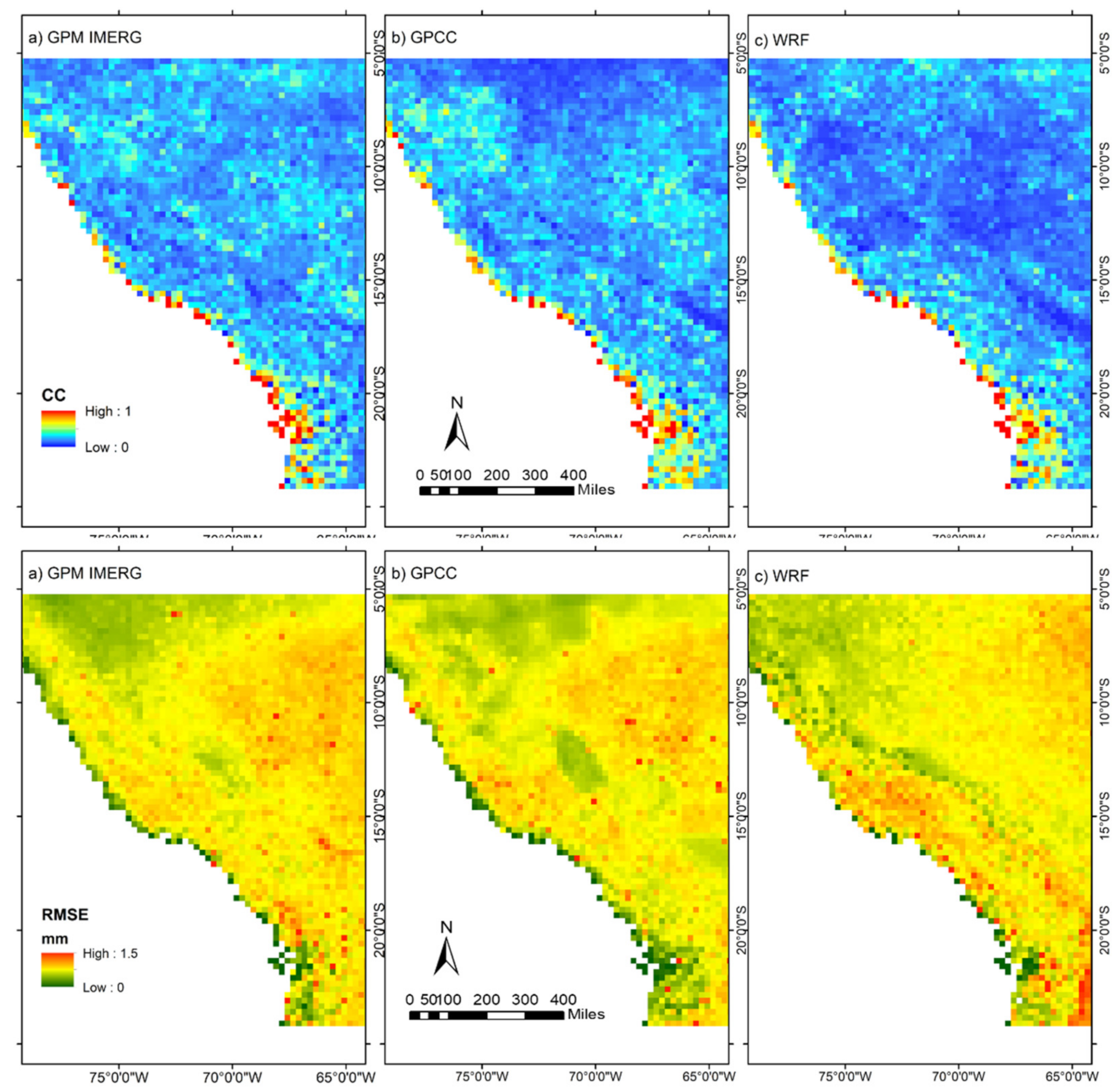
• GPM IMERG had more accurate precipitation estimates on the east slope (upwind) of the Andes than the west slope (downwind). IMERG had good performance over the Amazon basin. Considering that there is lack of human access and meteorological instruments in the Amazon rainforest, the GPM IMERG could be a useful dataset available for studies over the Amazon Basin.

This study provides a preliminary performance ranking of several global precipitation products over the mid-Andes region in South America. The study further analyzes the challenging area for precipitation estimates that was found in previous studies and finds the heterogeneity of uncertainties across climate zones of different precipitation products. The results can guide researchers to better select precipitation data with less uncertainties for their future studies. It also validates a WRF-based dynamic downscaling simulation over the same region, especially for the dryer regions of Peru and Chile, and such a dataset can be used to support local weather forecast and climate change studies.

References

1. Bayissa, Y.; Tadesse, T.; Demisse, G.; Shiferaw, A. Evaluation of Satellite-Based Rainfall Estimates and Application to Monitor Meteorological Drought for the Upper Blue Nile Basin, Ethiopia. Remote Sens. 2017, 9, 669. [Google Scholar] [CrossRef] [Green Version]
2. Garreaud, R.D.; Vuille, M.; Compagnucci, R.; Marengo, J. Present-Day South American Climate. Palaeogeogr. Palaeoclimatol. Palaeoecol. 2009, 281, 180–195. [Google Scholar] [CrossRef]
3. Hunziker, S.; Gubler, S.; Calle, J.; Moreno, I.; Andrade, M.; Velarde, F.; Ticona, L.; Carrasco, G.; Castellón, Y.; Oria, C.; et al. Identifying, Attributing, and Overcoming Common Data Quality Issues of Manned Station Observations: Identifying, Attributing, and Overcoming Common Data Quality Issues. Int. J. Climatol. 2017, 37, 4131–4145. [Google Scholar] [CrossRef] [Green Version]
4. Alijanian, M.; Rakhshandehroo, G.R.; Mishra, A.K.; Dehghani, M. Evaluation of Satellite Rainfall Climatology Using CMORPH, PERSIANN-CDR, PERSIANN, TRMM, MSWEP over Iran. Int. J. Clim. 2017, 37, 4896–4914. [Google Scholar] [CrossRef]
5. Huffman, G.; Bolvin, D.; Braithwaite, D.; Hsu, K.; Joyce, R.; Xie, P. Integrated Multi-SatellitE Retrievals for GPM (IMERG). In Vers. 4.4. NASA’s Precipitation Processing Center; NASA: Greenbelt, MD, USA, 2014. [Google Scholar]
6. Huffman, G.J.; Adler, R.F.; Morrissey, M.M.; Bolvin, D.T.; Curtis, S.; Joyce, R.; McGavock, B.; Suzzkind, J. Global Precipitation at One-Degree Daily Resolution from Multisatellite Observations. J. Hydrometeorol. 2001, 2, 36–50. [Google Scholar] [CrossRef]
7. Huffman, G.J.; Bolvin, D.T.; Braithwaite, D.; Hsu, K.; Joyce, R.; Kidd, C.; Nelkin, E.J.; Sorooshain, S.; Tan, J.; Xie, P. Developing the Integrated Multi-Satellite Retrievals for GPM (IMERG). In Proceedings of the EGU General Assembly, Vienna, Austria, 22–27 April 2012; EGU: Vienna, Austria, 2012; p. 6921. [Google Scholar]
8. Huffman, G.J.; Bolvin, D.T.; Nelkin, E.J.; Stocker, E.F.; Tan, J. V06 IMERG Release Notes, NASA, Greenbelt MD 2019. Available online: https://gpm.nasa.gov/resources/documents/imerg-v06-release-notes (accessed on 1 February 2022).
9. Joyce, R.J.; Janowiak, J.E.; Arkin, P.A.; Xie, P. CMORPH: A Method That Produces Global Precipitation Estimates from Passive Microwave and Infrared Data at High Spatial and Temporal Resolution. J. Hydrometeor 2004, 5, 487–503. [Google Scholar] [CrossRef]
10. Sorooshian, S.; Hsu, K.-L.; Gao, X.; Gupta, H.V.; Imam, B.; Braithwaite, D. Evaluation of PERSIANN System Satellite–Based Estimates of Tropical Rainfall. Bull. Amer. Meteor. Soc. 2000, 81, 2035–2046. [Google Scholar] [CrossRef]
11. Hong, Y.; Gochis, D.; Cheng, J.-T.; Hsu, K.; Sorooshian, S. Evaluation of PERSIANN-CCS Rainfall Measurement Using the NAME Event Rain Gauge Network. J. Hydrometeorol. 2007, 8, 469–482. [Google Scholar] [CrossRef] [Green Version]
12. Kubota, T.; Shige, S.; Hashizume, H.; Aonashi, K.; Takahashi, N.; Seto, S.; Hirose, M.; Takayabu, Y.N.; Ushio, T.; Nakagawa, K.; et al. Global Precipitation Map Using Satellite-Borne Microwave Radiometers by the GSMaP Project: Production and Validation. IEEE Trans. Geosci. Remote Sens. 2007, 45, 2259–2275. [Google Scholar] [CrossRef]
13. Derin, Y.; Anagnostou, E.; Berne, A.; Borga, M.; Boudevillain, B.; Buytaert, W.; Chang, C.-H.; Delrieu, G.; Hong, Y.; Hsu, Y.C.; et al. Multiregional Satellite Precipitation Products Evaluation over Complex Terrain. J. Hydrometeorol. 2016, 17, 1817–1836. [Google Scholar] [CrossRef]
14. Derin, Y.; Anagnostou, E.; Berne, A.; Borga, M.; Boudevillain, B.; Buytaert, W.; Chang, C.-H.; Chen, H.; Delrieu, G.; Hsu, Y.; et al. Evaluation of GPM-Era Global Satellite Precipitation Products over Multiple Complex Terrain Regions. Remote Sens. 2019, 11, 2936. [Google Scholar] [CrossRef] [Green Version]
15. Schneider, U.; Becker, A.; Finger, P.; Rustemeier, E.; Ziese, M. GPCC Full Data Monthly Version 2020 at 0.25°: Monthly Land-Surface Precipitation from Rain-Gauges Built on GTS-Based and Historic Data: Gridded Monthly Totals 2020, 5 MB–300 MB per Gzip Compressed NetCDF File; GPCC: Green Point, Australia, 2020. [Google Scholar]
16. Schneider, U.; Becker, A.; Finger, P.; Meyer-Christoffer, A.; Ziese, M.; Rudolf, B. GPCC’s New Land Surface Precipitation Climatology Based on Quality-Controlled In Situ Data and Its Role in Quantifying the Global Water Cycle. Appl. Clim. 2014, 115, 15–40. [Google Scholar] [CrossRef] [Green Version]
17. Schneider, U.; Becker, A.; Finger, P.; Meyer-Christoffer, A.; Rudolf, B.; Ziese, M. GPCC Full Data Reanalysis Version 7.0 at 0.5°: Monthly Land-Surface Precipitation from Rain-Gauges Built on GTS-Based and Historic Data: Gridded Monthly Totals 2015, 20–270 MB per Decadal Gzip Compressed NetCDF Archive; GPCC: Green Point, Australia, 2016. [Google Scholar]
18. Wang, G.; Zhang, P.; Liang, L.; Zhang, S. Evaluation of Precipitation from CMORPH, GPCP-2, TRMM 3B43, GPCC, and ITPCAS with Ground-Based Measurements in the Qinling-Daba Mountains, China. PLoS ONE 2017, 12, e0185147. [Google Scholar] [CrossRef] [Green Version]
19. Aybar, C.; Fernández, C.; Huerta, A.; Lavado, W.; Vega, F.; Felipe-Obando, O. Construction of a High-Resolution Gridded Rainfall Dataset for Peru from 1981 to the Present Day. Hydrol. Sci. J. 2020, 65, 770–785. [Google Scholar] [CrossRef]
20. Funk, C.; Peterson, P.; Landsfeld, M.; Pedreros, D.; Verdin, J.; Shukla, S.; Husak, G.; Rowland, J.; Harrison, L.; Hoell, A.; et al. The Climate Hazards Infrared Precipitation with Stations—A New Environmental Record for Monitoring Extremes. Sci. Data 2015, 2, 150066. [Google Scholar] [CrossRef] [Green Version]
21. Beck, H.E.; Wood, E.F.; Pan, M.; Fisher, C.K.; Miralles, D.G.; van Dijk, A.I.J.M.; McVicar, T.R.; Adler, R.F. MSWEP V2 Global 3-Hourly 0.1° Precipitation: Methodology and Quantitative Assessment. Bull. Am. Meteorol. Soc. 2019, 100, 473–500. [Google Scholar] [CrossRef] [Green Version]
22. Lundquist, J.; Hughes, M.; Gutmann, E.; Kapnick, S. Our Skill in Modeling Mountain Rain and Snow Is Bypassing the Skill of Our Observational Networks. Bull. Am. Meteorol. Soc. 2019, 100, 2473–2490. [Google Scholar] [CrossRef] [Green Version]
23. Leung, L.R.; Qian, Y. The Sensitivity of Precipitation and Snowpack Simulations to Model Resolution via Nesting in Regions of Complex Terrain. J. Hydrometeor 2003, 4, 1025–1043. [Google Scholar] [CrossRef]
24. Soares, P.M.M.; Cardoso, R.M.; Miranda, P.M.A.; de Medeiros, J.; Belo-Pereira, M.; Espirito-Santo, F. WRF High Resolution Dynamical Downscaling of ERA-Interim for Portugal. Clim. Dyn. 2012, 39, 2497–2522. [Google Scholar] [CrossRef]
25. Zhang, Z.; Arnault, J.; Laux, P.; Ma, N.; Wei, J.; Shang, S.; Kunstmann, H. Convection-Permitting Fully Coupled WRF-Hydro Ensemble Simulations in High Mountain Environment: Impact of Boundary Layer- and Lateral Flow Parameterizations on Land–Atmosphere Interactions. Clim. Dyn. 2021, 59, 1355–1376. [Google Scholar] [CrossRef]
26. Posada-Marín, J.A.; Rendón, A.M.; Salazar, J.F.; Mejía, J.F.; Villegas, J.C. WRF Downscaling Improves ERA-Interim Representation of Precipitation around a Tropical Andean Valley during El Niño: Implications for GCM-Scale Simulation of Precipitation over Complex Terrain. Clim. Dyn. 2019, 52, 3609–3629. [Google Scholar] [CrossRef]
27. Peel, M.C.; Finlayson, B.L.; McMahon, T.A. Updated World Map of the Köppen-Geiger Climate Classification. Hydrol. Earth Syst. Sci. 2007, 11, 1633–1644. [Google Scholar] [CrossRef] [Green Version]
28. Beck, H.E.; Zimmermann, N.E.; McVicar, T.R.; Vergopolan, N.; Berg, A.; Wood, E.F. Present and Future Köppen-Geiger Climate Classification Maps at 1-Km Resolution. Sci. Data 2018, 5, 180214. [Google Scholar] [CrossRef] [Green Version]
29. Lavado Casimiro, W.S.; Ronchail, J.; Labat, D.; Espinoza, J.C.; Guyot, J.L. Basin-Scale Analysis of Rainfall and Runoff in Peru (1969–2004): Pacific, Titicaca and Amazonas Drainages. Hydrol. Sci. J. 2012, 57, 625–642. [Google Scholar] [CrossRef] [Green Version]
30. Viale, M.; Bianchi, E.; Cara, L.; Ruiz, L.E.; Villalba, R.; Pitte, P.; Masiokas, M.; Rivera, J.; Zalazar, L. Contrasting Climates at Both Sides of the Andes in Argentina and Chile. Front. Environ. Sci. 2019, 7, 69. [Google Scholar] [CrossRef] [Green Version]
31. Manz, B.; Páez-Bimos, S.; Horna, N.; Buytaert, W.; Ochoa-Tocachi, B.; Lavado-Casimiro, W.; Willems, B. Comparative Ground Validation of IMERG and TMPA at Variable Spatiotemporal Scales in the Tropical Andes. J. Hydrometeorol. 2017, 18, 2469–2489. [Google Scholar] [CrossRef]
32. Chang, N.-B.; Hong, Y. (Eds.) Multiscale Hydrologic Remote Sensing: Perspectives and Applications; Taylor & Francis: Boca Raton, FL, USA, 2012; ISBN 978-1-4398-7745-6. [Google Scholar]
33. Hou, A.Y.; Kakar, R.K.; Neeck, S.; Azarbarzin, A.A.; Kummerow, C.D.; Kojima, M.; Oki, R.; Nakamura, K.; Iguchi, T. The Global Precipitation Measurement Mission. Bull. Am. Meteorol. Soc. 2014, 95, 701–722. [Google Scholar] [CrossRef]
34. Huffman, G.J.; Bolvin, D.T.; Braithwaite, D.; Hsu, K.; Joyce, R.; Kidd, C.; Nelkin, E.J.; Sorooshian, S.; Tan, J.; Xie, P. Algorithm Theoretical Basis Document (ATBD) Version 06 NASA Global Precipitation Measurement (GPM) Integrated Multi-SatellitE Retrievals for GPM (IMERG); NASA: Greenbelt, MD, USA, 2019. [Google Scholar]
35. Xu, Z.; Wu, Z.; He, H.; Wu, X.; Zhou, J.; Zhang, Y.; Guo, X. Evaluating the Accuracy of MSWEP V2.1 and Its Performance for Drought Monitoring over Mainland China. Atmos. Res. 2019, 226, 17–31. [Google Scholar] [CrossRef]
36. Liu, J.; Shangguan, D.; Liu, S.; Ding, Y.; Wang, S.; Wang, X. Evaluation and Comparison of CHIRPS and MSWEP Daily-Precipitation Products in the Qinghai-Tibet Plateau during the Period of 1981–2015. Atmos. Res. 2019, 230, 104634. [Google Scholar] [CrossRef]
37. Nair, A.; Indu, J. Performance Assessment of Multi-Source Weighted-Ensemble Precipitation (MSWEP) Product over India. Climate 2017, 5, 2. [Google Scholar] [CrossRef]
38. Lo Conti, F.; Hsu, K.-L.; Noto, L.V.; Sorooshian, S. Evaluation and Comparison of Satellite Precipitation Estimates with Reference to a Local Area in the Mediterranean Sea. Atmos. Res. 2014, 138, 189–204. [Google Scholar] [CrossRef] [Green Version]
39. Hu, Z.; Zhou, Q.; Chen, X.; Li, J.; Li, Q.; Chen, D.; Liu, W.; Yin, G. Evaluation of Three Global Gridded Precipitation Data Sets in Central Asia Based on Rain Gauge Observations. Int. J. Clim. 2018, 38, 3475–3493. [Google Scholar] [CrossRef]
40. Basheer, M.; Elagib, N.A. Performance of Satellite-Based and GPCC 7.0 Rainfall Products in an Extremely Data-Scarce Country in the Nile Basin. Atmos. Res. 2019, 215, 128–140. [Google Scholar] [CrossRef]
41. Skamarock, W.C.; Klemp, J.B.; Dudhia, J.; Gill, D.O.; Liu, Z.; Berner, J.; Wang, W.; Powers, J.G.; Duda, M.G.; Barker, D.M.; et al. A Description of the Advanced Research WRF Model Version 4; UCAR/NCAR: Boulder, CO, USA, 2019. [Google Scholar]
42. Hersbach, H.; Bell, B.; Berrisford, P.; Hirahara, S.; Horányi, A.; Muñoz-Sabater, J.; Nicolas, J.; Peubey, C.; Radu, R.; Schepers, D.; et al. The ERA5 Global Reanalysis. Q. J. R. Meteorol. Soc. 2020, 146, 1999–2049. [Google Scholar] [CrossRef]
43. Thompson, G.; Field, P.R.; Rasmussen, R.M.; Hall, W.D. Explicit Forecasts of Winter Precipitation Using an Improved Bulk Microphysics Scheme. Part II: Implementation of a New Snow Parameterization. Mon. Weather Rev. 2008, 136, 5095–5115. [Google Scholar] [CrossRef]
44. Hong, S.-Y.; Lim, J.-O.J. The WRF Single-Moment 6-Class Microphysics Scheme (WSM6). J. Korean Meteorol. Soc. 2006, 42, 129–151. [Google Scholar]
45. Iacono, M.J.; Delamere, J.S.; Mlawer, E.J.; Shephard, M.W.; Clough, S.A.; Collins, W.D. Radiative Forcing by Long-Lived Greenhouse Gases: Calculations with the AER Radiative Transfer Models. J. Geophys. Res. 2008, 113, D13103. [Google Scholar] [CrossRef]
46. Ek, M.B.; Mitchell, K.E.; Lin, Y.; Rogers, E.; Grunmann, P.; Koren, V.; Gayno, G.; Tarpley, J.D. Implementation of Noah Land Surface Model Advances in the National Centers for Environmental Prediction Operational Mesoscale Eta Model. J. Geophys. Res. 2003, 108, 2002JD003296. [Google Scholar] [CrossRef]
47. Niu, G.-Y.; Yang, Z.-L.; Mitchell, K.E.; Chen, F.; Ek, M.B.; Barlage, M.; Kumar, A.; Manning, K.; Niyogi, D.; Rosero, E.; et al. The Community Noah Land Surface Model with Multiparameterization Options (Noah-MP): 1. Model Description and Evaluation with Local-Scale Measurements. J. Geophys. Res. 2011, 116, D12109. [Google Scholar] [CrossRef] [Green Version]
48. Jiménez, P.A.; Dudhia, J.; González-Rouco, J.F.; Navarro, J.; Montávez, J.P.; García-Bustamante, E. A Revised Scheme for the WRF Surface Layer Formulation. Mon. Weather Rev. 2012, 140, 898–918. [Google Scholar] [CrossRef] [Green Version]
49. Tiedtke, M. A Comprehensive Mass Flux Scheme for Cumulus Parameterization in Large-Scale Models. Mon. Wea. Rev. 1989, 117, 1779–1800. [Google Scholar] [CrossRef]
50. Moriasi, D.N.; Arnold, J.G.; Van Liew, M.W.; Bingner, R.L.; Harmel, R.D.; Veith, T.L. Veith Model Evaluation Guidelines for Systematic Quantification of Accuracy in Watershed Simulations. Trans. ASABE 2007, 50, 885–900. [Google Scholar] [CrossRef]
51. Burgan, H.I.; Aksoy, H. Daily Flow Duration Curve Model for Ungauged Intermittent Subbasins of Gauged Rivers. J. Hydrol. 2022, 604, 127249. [Google Scholar] [CrossRef]
52. Li, C.; Tang, G.; Hong, Y. Cross-Evaluation of Ground-Based, Multi-Satellite and Reanalysis Precipitation Products: Applicability of the Triple Collocation Method across Mainland China. J. Hydrol. 2018, 562, 71–83. [Google Scholar] [CrossRef]
53. Li, Z.; Chen, M.; Gao, S.; Hong, Z.; Tang, G.; Wen, Y.; Gourley, J.J.; Hong, Y. Cross-Examination of Similarity, Difference and Deficiency of Gauge, Radar and Satellite Precipitation Measuring Uncertainties for Extreme Events Using Conventional Metrics and Multiplicative Triple Collocation. Remote Sens. 2020, 12, 1258. [Google Scholar] [CrossRef] [Green Version]
54. Yilmaz, M.T.; Crow, W.T. Evaluation of Assumptions in Soil Moisture Triple Collocation Analysis. J. Hydrometeorol. 2014, 15, 1293–1302. [Google Scholar] [CrossRef]
55. Zwieback, S.; Scipal, K.; Dorigo, W.; Wagner, W. Structural and Statistical Properties of the Collocation Technique for Error Characterization. Nonlin. Process. Geophys. 2012, 19, 69–80. [Google Scholar] [CrossRef]
56. Tian, Y.; Huffman, G.J.; Adler, R.F.; Tang, L.; Sapiano, M.; Maggioni, V.; Wu, H. Modeling Errors in Daily Precipitation Measurements: Additive or Multiplicative. Geophys. Res. Lett. 2013, 40, 2060–2065. [Google Scholar] [CrossRef] [Green Version]
57. Alemohammad, S.H.; McColl, K.A.; Konings, A.G.; Entekhabi, D.; Stoffelen, A. Characterization of Precipitation Product Errors across the United States Using Multiplicative Triple Collocation. Hydrol. Earth Syst. Sci. 2015, 19, 3489–3503. [Google Scholar] [CrossRef] [Green Version]
58. Yu, Y.; Schneider, U.; Yang, S.; Becker, A.; Ren, Z. Evaluating the GPCC Full Data Daily Analysis Version 2018 through ETCCDI Indices and Comparison with Station Observations over Mainland of China. Appl. Clim. 2020, 142, 835–845. [Google Scholar] [CrossRef]
59. Salati, E.; Vose, P.B. Amazon Basin: A System in Equilibrium. Science 1984, 225, 129–138. [Google Scholar] [CrossRef]
60. Schulz-Stellenfleth, J.; Staneva, J. A Multi-Collocation Method for Coastal Zone Observations with Applications to Sentinel-3A Altimeter Wave Height Data. Ocean Sci. 2019, 15, 249–268. [Google Scholar] [CrossRef] [Green Version]
61. Gruber, A.; Dorigo, W.A.; Crow, W.; Wagner, W. Triple Collocation-Based Merging of Satellite Soil Moisture Retrievals. IEEE Trans. Geosci. Remote Sens. 2017, 55, 6780–6792. [Google Scholar] [CrossRef]
Figure 1. The study area and the Köppen–Geiger–Pohl climate zones in the study area.
Atmosphere 13 01666 g001
Figure 2. The schematic flowchart of the analysis in this study.
Atmosphere 13 01666 g002
Figure 3. The 10-year average annual precipitation from 2010 to 2019 of (a) GPM IMERG, (b) MSWEP, (c) WRF simulation, and (d) GPCC.
Atmosphere 13 01666 g003
Figure 4. The map of daily precipitation statistical comparison of (a) GPM IMERG, (b) MSWEP, and (c) WRF simulation with rain gauge data from January 2010 to July 2018 in the Peruvian region.
Atmosphere 13 01666 g004
Figure 5. The violin plot of statistical results (a,c,e) from GPM IMERG, MSWEP, and WRF simulations in the Peruvian region. The subplots of statistical results in different climate zones are listed in (b,d,f). The cross bar in the inside box within the violin plot is the median, and the vertical length of the box indicates the confidence interval of the sample.
Atmosphere 13 01666 g005
Figure 6. The cross examination of GPM IMERG, MSWEP, and WRF simulation at 6 h time steps from 2010 to 2019. The name on the right side of “-“ is the “reference data product” in the calculation.
Atmosphere 13 01666 g006
Figure 7. The violin plot of cross-examination between GPM IMERG, MSWEP, and WRF simulations in six major climate zones, where (a,c,e) are the aggregated statistic for CC, NB, and RMSE, and (b,d,f) are the statistic at each climate zone.
Atmosphere 13 01666 g007
Figure 8. The MTC analysis results (CC and RMSE) between (a) GPM IMERG, (b) GPCC, and (c) WRF at a monthly time scale from 2010 to 2019.
Atmosphere 13 01666 g008
Figure 9. The violin plot of MTC analysis results (a,c) for GPM IMERG, GPCC, and WRF simulations from 2010 to 2019 at a monthly scale, and the breakdown results (b,d) based on their averaged annual precipitation amount.
Atmosphere 13 01666 g009