Article

Role of the Observability Gramian in Parameter Estimation: Application to Nonchaotic and Chaotic Systems via the Forward Sensitivity Method †

by
John M. Lewis
1,2,* and
Sivaramakrishnan Lakshmivarahan
3
1
National Severe Storms Laboratory, Norman, OK 73072, USA
2
Desert Research Institute, Reno, NV 89512, USA
3
School of Computer Science, University of Oklahoma, Norman, OK 73069, USA
*
Author to whom correspondence should be addressed.
This paper is dedicated to the memory of Sherry Lynn Lewis.
Atmosphere 2022, 13(10), 1647; https://doi.org/10.3390/atmos13101647
Submission received: 16 August 2022 / Revised: 27 September 2022 / Accepted: 28 September 2022 / Published: 10 October 2022

Abstract

:
Data assimilation in chaotic regimes is challenging, and among the challenging aspects is placement of observations to induce convexity of the cost function in the space of control. This problem is examined by using Saltzman’s spectral model of convection that admits both chaotic and nonchaotic regimes and is controlled by two parameters—Rayleigh and Prandtl numbers. The problem is simplified by stripping the seven-variable constraint to a three-variable constraint. Since emphasis is placed on observation positioning to avoid cost-function flatness, forecast sensitivity to controls is needed. Four-dimensional variational assimilation (4D-Var) is silent on this issue of observation placement while Forecast Sensitivity Method (FSM) delivers sensitivities used in placement. With knowledge of the temporal forecast sensitivity matrix V , derivatives of the forecast variables to controls, the cost function can be expressed as a function of the observability Gramian V T V using first-order Taylor series expansion. The goal is to locate observations at places that force the Gramian positive definite. Further, locations are chosen such that the condition number of V T V is small and this guarantees convexity in the vicinity of the cost function minimum. Four numerical experiments are executed, and results are compared with the structure of the cost function independently determined though arduous computation over a wide range of the two nondimensional numbers. The results are especially good based on reduction in cost function value and comparison with cost function structure.

1. Introduction

In his pioneering work, Saltzman [1] derived the well-known spectral model of Rayleigh–Bénard convection [2,3]. It was a 7-variable double Fourier series representation of the convection herein called Saltzman’s low-order model and denoted by S-LOM (7). His model included a single parameter, the Rayleigh number R . In the governing equations, the ratio of the Rayleigh number to the critical Rayleigh number R c , λ = R R c , becomes the key parameter. He assumed the other nondimensional number associated with this convection problem, the Prandtl number σ ,   was set equal to 10. Historically, Saltzman’s [1] model achieved fame by providing Lorenz [4] with a nonlinear deterministic model that exhibits nonperiodic solution to explore the limitations of extended-range predictability. Within a decade, Lorenz’s three-variable version of Saltzman’s model became known as the chaotic-butterfly model [5], so-named because the phase-space depiction of model evolution resembled butterfly wings.
The goal of the research is to explore data assimilation [6] for the Rayleigh–Bénard convection in both chaotic and nonchaotic regimes. Two three-variable stripped-down versions of S-LOM (7) are used as dynamical constraints: (1) S-LOM (3) based on Saltzman’s scaling, and L-LOM (3) based on Lorenz’s scaling. These truncated systems contain the ingredients central to defining observation placement that yield a cost function minimum. The strength of this methodology rests on expressing the cost function (to a first-order accuracy around the true but unknown minimum) as a quadratic function of the increment in the control variable with (the symmetric and positive semi-definite) observability Gramian as the matrix of this approximate quadratic function. It is shown that by choosing the observation sites that maximize the square of the forecast sensitivities to control, we can indeed force the observability Gramian to be a positive definite matrix. This in turn avoids the occurrence of flat patches of the cost function in the control space. Refer to Lakshmivarahan et al. [7,8] and Lewis et al. [9] for further details and applications. An alternate strategy would be to place observations at locations that would lead to a small condition number for the observability Gramian.
Following this Introduction, we summarize S-LOM (7) and its reduction to the three-variable form [10] in Section 2. In Section 2, we also give attention to the scaling of S-LOM (3) and L-LOM (3). Discussion of the three-variable spectral dynamics is presented alongside graphics for nonchaotic and chaotic regimes in Section 3. Mechanics for data assimilation follow in Section 4. Data assimilation experiments are executed in Section 5, and discussion along with conclusions end the paper in Section 6.

2. Three-Variable Forms of Saltzman’s Model

2.1. Spectral Form of Solution

The laboratory experiments of Bénard [2] were conducted with a rigid surface (a metal plate) below and a free upper surface while later experimental investigations used rigid surfaces at top and below (Chandrasekhar 1961 [11], Ch. 2, sect. 18c; Turner 1973 [12], Ch. 7, sect. 7.2). Saltzman’s [1] theoretical development assumed two free surfaces. The onset of convection has different critical Rayleigh numbers R c associated with the various boundary conditions—roughly 600 for free surfaces, 1800 for rigid surfaces, and 1200 for one-free and one-rigid surface. We use the free-surfaces value of R c = 657.5 to develop the data assimilation model.
In an earlier technical report by the authors (Lewis and Lakshmivarahan [13]), a re-derivation of S-LOM (7) led to functional forms of coefficients in the equations that governed the Fourier amplitudes. As it stood in Saltzman’s paper [1], the coefficients were expressed in numerical values only. Since our goal was to use Saltzman’s equations in FSM data assimilation with the two nondimensional numbers as parameters, we needed to know the coefficients in terms of the wavenumbers and variable nondimensional numbers.
The three-variable form of Saltzman’s equations used in this study is a subset of his seven-variable form. By setting the initial condition on the 3-horizontal wave temperature departure to 1 while the other initial conditions are set to zero delivers the three-variable form involving the (horizontal wavenumber 3/vertical wavenumber 1) streamfunction, the (horizontal wavenumber 3/vertical wavenumber 1) temperature departure, and the (vertical wavenumber 2) temperature departure. Let us label the three amplitudes in S-LOM (3) as follows: x 1 for the streamfunction (corresponding to amplitude A in Saltzman’s notation). Temperature-departure components x 4 and x 7 (corresponding to amplitudes D and G in Saltzman’ notation). This revised notation is consistent with the ordering of coefficients from 1 to 7 in Lewis and Lakshmivarahan [13] where x 1 ,   x 2 ,   ,   x 7 replaced A, B, …, G.
The streamfunction ψ in S-LOM (3) is given by
ψ ( x , z , t ) = 4 x 1 ( t ) sin ( π a x ) sin ( π z )  
where a ,   the nondimensional wavenumber, is given by a = 1 2 which defines the 3-horizontal wavenumber wave, and the temperature departure θ is given by
θ ( x , z , t ) = 4 x 4 ( t ) cos ( π a x ) sin ( π z ) + 4 x 7 ( t ) sin ( 2 π z )  

2.2. Amplitude Equations

When Equations (1) and (2) are substituted into the partial differential equations that govern Rayleigh–Bénard convection, the two-dimensional (x, z) vorticity equation and the temperature departure equation, followed by imposition of integral orthogonality conditions for the double Fourier series, ordinary differential equations governing the time-dependent amplitudes follow where we have expressed coefficients to two decimal places (same accuracy as used by Saltzman [1]):
Saltzman’s S-LOM (3) equations:
x 1 ˙ = σ π 2 ( 1 + a 2 ) x 1 σ a x 4 π ( 1 + a 2 )   = 14.80 σ   x 1 0.15 σ x 4
x 4 ˙ = 4 π 2 a x 1 x 4 π a R c λ x 1 π 2 ( 1 + a 2 ) x 4 = 27.92 x 1 x 7 1460.62 λ x 1 14.80 x 4
x 7 ˙ = 2 π 2 a x 1 x 4 4 π 2 x 7 = 13.96 x 1 x 4 39.48 x 7
where
λ = R R c   ( R : R a y l e i g h   number )  
Lorenz [4] used another scaling for the derivation of his L-LOM (3) that took the form:
Lorenz’s L-LOM (3) equations:
x 1 ˙ = σ x 1 + σ x 4  
x 4 ˙ = x 1 x 7 + λ x 1 x 4  
x 7 ˙ = x 1 x 4 b x 7  
where
b = 4 1 + a 2 = 8 3  
Table 1 shows non-dimensional and scaling for S-LOM (3) and L-LOM (3). The different signs on the right-hand sides of S-LOM (3) and L-LOM (3) stem from the fact that Lorenz assumed double Fourier representation of temperature departure and streamfunction as follows:
θ ( x , z , t ) = x 4 ( t ) cos ( π a x ) sin ( π z ) x 7 ( t ) sin ( 2 π z )    
ψ ( x , z , t ) = x 1 ( t ) sin ( π a x ) sin ( π z )
where the sign of the x 7 -component term in Equation (11) is opposite the corresponding term in Equation (2) and the sign of the streamfunction in Equation (12) is opposite the sign in Equation (1). These sign differences lead to a shift of temperature departure structure relative to the streamfunction structure in the convective regime compared to Saltzman’s results. However, temperature–motion structures in S-LOM (3) and L-LOM (3) are both faithful to Rayleigh–Bénard cellular convection.
1 ( 1 + a 2 ) π 2 = 0.068 ;     1 + a 2 a = 2.121 ;   [ π ( 1 + a 2 ) ] 3 a 2 = 209.292    
If the physical parameters are taken to be those associated with water at 20 °C (Chandrasekhar [11] (1961, Ch. 2, Table V1), the physical parameters are given by
ν = 1.006 · 10 2   cm 2   sec 1 κ = 1.433 · 10 3   cm 2   sec 1 ϵ = 2.0 · 10 3   ° C 1
In laboratory experiments, the fluid height falls between 2   mm   and   1   cm   (Chandrasekhar 1961 [11], Ch. 2, sect. 18). Let us assume H = 2   mm . Then, the relative values of Saltzman’s and Lorenz’s nondimensional variables follow:
  • Lorenz’s nondimensional t * is roughly 15 times greater than Saltzman’s nondimensional t * ,
  • Lorenz’s nondimensional x * and z * are equal to Saltzman’s nondimensional x * and z * ,
  • Lorenz’s nondimensional ψ * is roughly 2 times less than Saltzman’s nondimensional ψ * , and
  • Lorenz’s nondimensional θ * is roughly 200 times less than Saltzman’s nondimensional θ *
Thus, for example, if the nonchaotic convective regime comes to equilibrium at Lorenz’s t * = 15 ,   it comes to equilibrium at Saltzman’s t * = 1 . Similarly, a temperature departure of θ * = 200 in Saltzman’s case is associated with Lorenz’s value of θ * = 1 .
The equations governing the evolution of forecast sensitivities are found by taking partial derivatives of S-LOM (3) and L-LOM (3) with respect to λ   and   σ separately. Thus, six equations are added to each set, S-LOM (3) and S-LOM (3).
We demonstrate the process of determining evolution of forecast sensitivities by deriving the equation governing for x 4 λ :
x 4 ˙ = d x 4 d t = x 1 x 7 + λ x 1 x 4 d d t ( x 4 λ ) = x 1 x 7 λ x 7 x 1 λ + x 1 + λ x 1 λ x 4 λ
Similar ordinary differential equations are derived for the other forecast sensitivities. The initial conditions for the six sensitivity equations are zero, i.e., change in controls λ   and   σ affect the sensitivity solutions for t > 0 ,   but not at t = 0 . The 3-variable amplitude solutions feed into the forecast sensitivity equations as shown in Equation (15), but the forecast sensitivity equations do not feedback into the equations governing x 1 , x 4 ,   and   x 7 . The set of nine differential equations are solved simultaneously as a coupled set.

3. Dynamics of 3-Mode Systems: S-LOM (3) and L-LOM (3)

3.1. Overview

The 3-mode truncated systems that describe Rayleigh–Bénard convection have similar strength (they capture the interaction between temperature and vorticity that produce the physically meaningful convective motions) and similar weakness (inability to depict turbulent cellular motion with limited wave structures in the presence of large Rayleigh numbers). However, it is the difference in scaling and nondimensional forms that highlights the dynamical difference in the equation sets. It would be interesting to ask Lorenz why he refused to follow Saltzman’s scaling and associated coefficients for the differential equations plainly set forth in Saltzman’s Table 2 [1] One can guess that he wanted differential equations where the coefficients exhibited comparable magnitudes that lead to ease in understanding interaction between terms in the equation set. However, beyond this difference, the model forecast sensitivities to controls are drastically different between the two sets—relatively large model forecast sensitivity to controls in S-LOM (3)’s case compared to L-LOM (3)’s case. These differences lead to poor data assimilation results when slight changes in ideal observation times are used in the S-LOM (3) experiments. On the other hand, L-LOM (3) tolerated these slight changes very well. Results of these experiments are discussed in Section 5.1 (L-LOM (3) dynamics) and Section 5.2 (S-LOM (3) dynamics). All calculations in Section 3.2 and Section 3.3 use L-LOM (3).

3.2. Nonchaotic Regime: λ = 12 , σ = 7 ( σ = ν κ = 7.03 for Water at 20   ° C )

When λ = 12 ,   the Rayleigh number R is given by
R = λ R c = 12   ( 657.5 ) = 8.106 · 10 3
With this value of R and H   = 2   mm for water at 20   ° C ,   Rayleigh’s [3] formula for the temperature difference T between the upper and lower boundaries of the fluid is given by
T = κ ν R g ϵ H 3 = 7.11   ° C
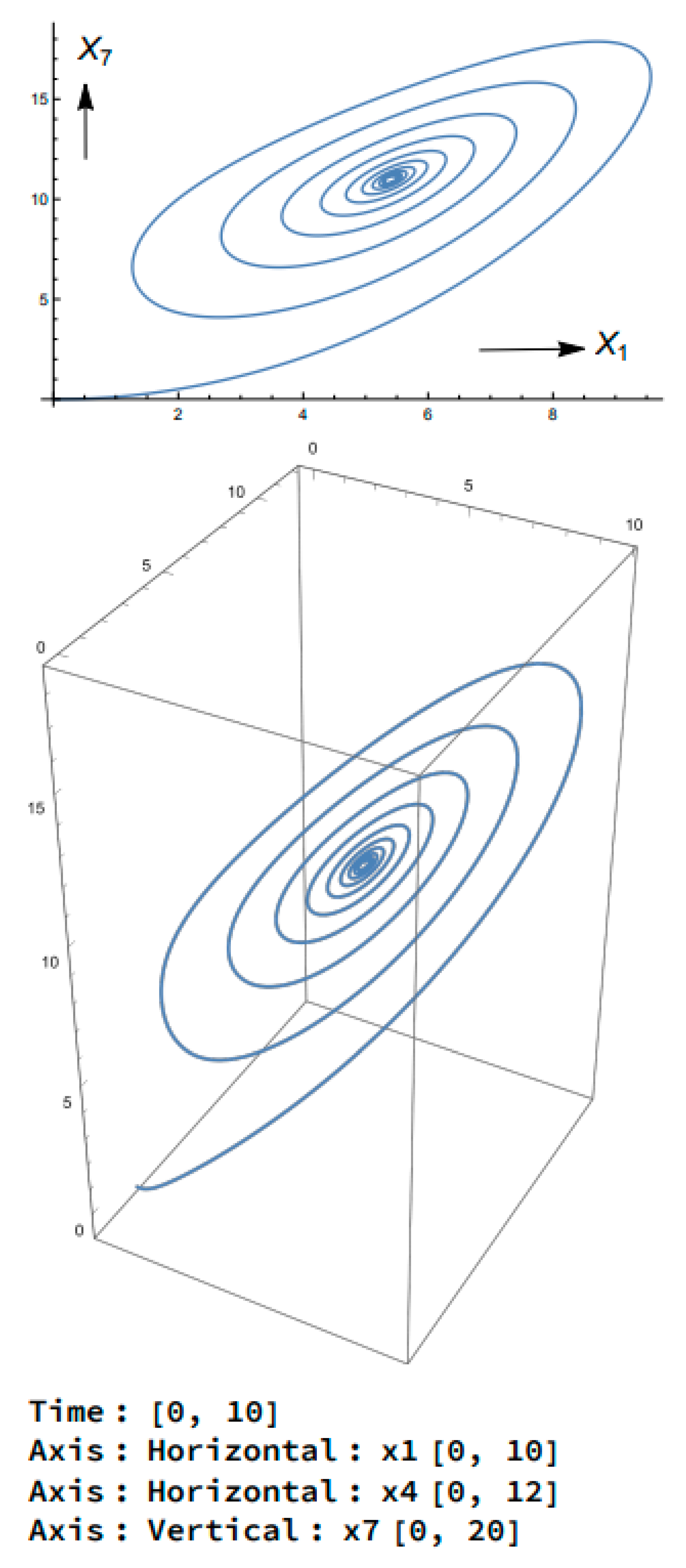
In the first three panels of Figure 1, amplitudes are depicted in pairs between t = 0   and   t = 10   ( 5 min dimensionally ) : x 1 x 4 (first panel, top), x 4 x 7 ( second panel), and x 1 x 7 (third panel). In each of these panels, amplitudes are oscillatory and exhibit convergence to x 1 5.50 ,   x 4 = 5.75 ,   and   x 7 = 12.0 . In the bottom panel of Figure 1, the 3D trajectory of the amplitudes in phase space—( λ ,   σ ) space—is shown over the period t = 0   to   t = 10 . This plot indicates convergence of L-LOM (3) to the x 1 ,   x 4 ,   x 7 values stated above.
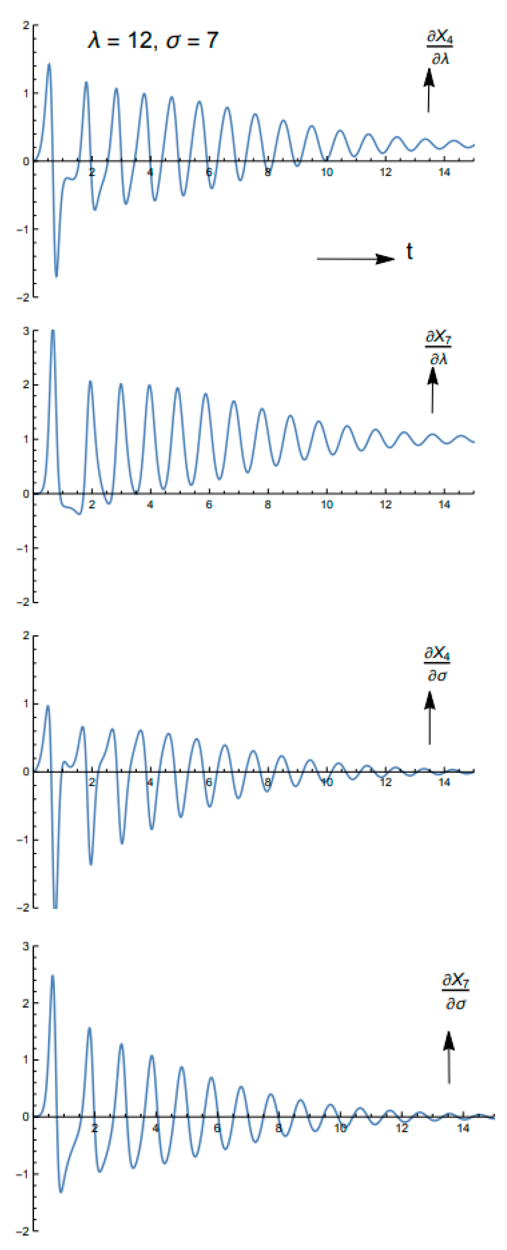
The forecast sensitivities of x 4   and   x 7 with respect to λ   and   σ are shown in Figure 2. These two amplitude components are used to represent the temperature departure, and since only temperature departure observations will be used in the data assimilation experiments, we confine our forecast sensitivity analysis to these two components. These sensitivities exhibit oscillatory decay as steady state is approached.
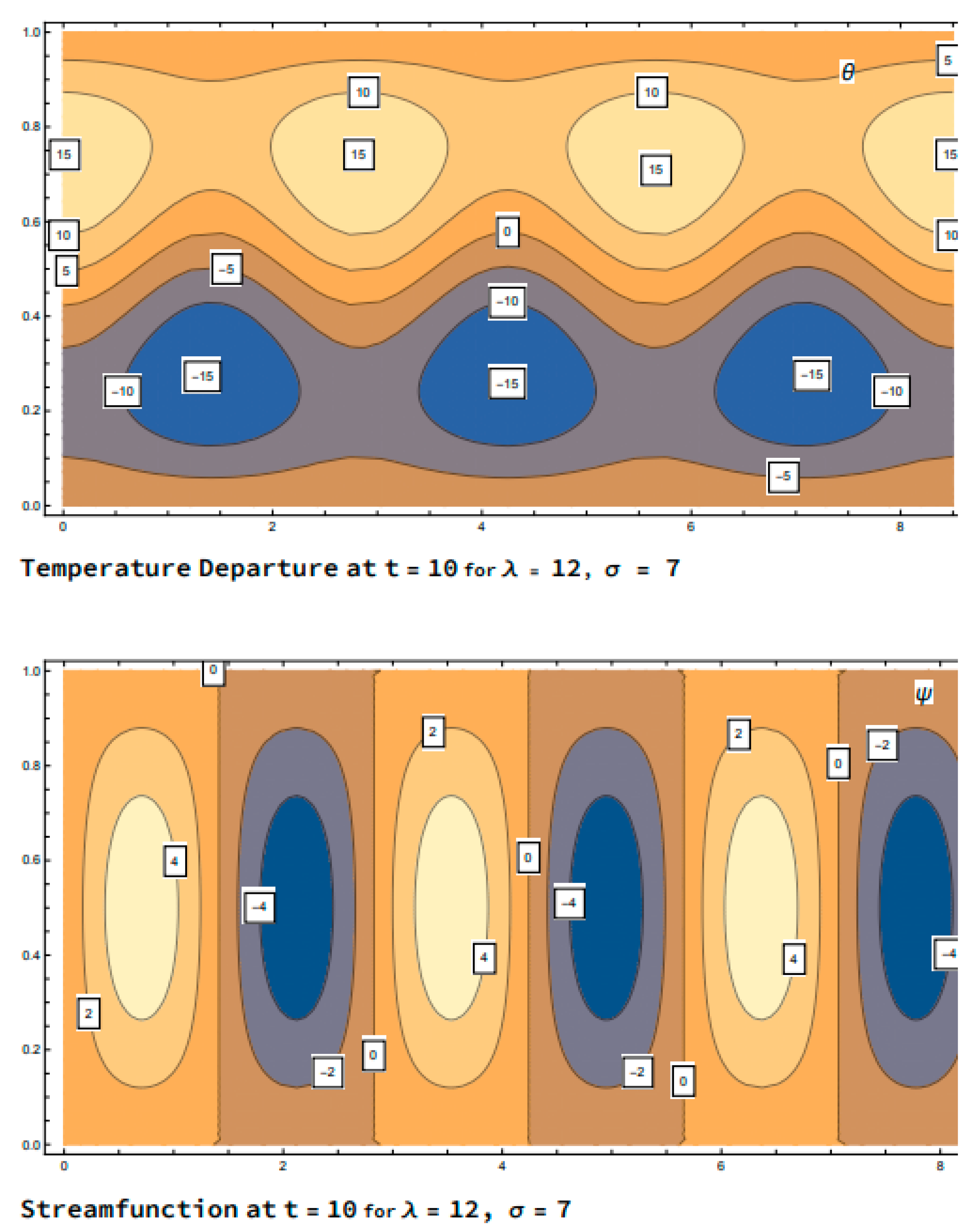
The structure of the convection at t = 10   is shown in Figure 3—two panels, the temperature departure and streamfunction. The maximum/minimum values of temperature departure are ~ ± 15 ( ± 3   ° C   dimensionally for water at 20   ° C ) where the maximum values are in the top portion of the water and the minimum values in the bottom portion. This leads to a spurious stable stratification first noted by Kuo [14] when convection is controlled by a truncated low-order spectral system. Within the cells, the maximum ( ψ x > 0 )   and minimum ( ψ x < 0 )   upward/downward vertical velocities, respectively, are the order of 1   mm · s 1 so roughly 50 circuits of a fluid particle around the cell takes place between the onset of convective motion ( t = 0 ) and steady state ( t = 10 ) .

3.3. Chaotic Regime: λ = 28 , σ = 10

The Prandtl number σ = 10 was assumed by Saltzman [1] in nonchaotic regimes and by Lorenz [4] in chaotic regimes. With these nondimensional numbers, Lorenz [4] found that instability of steady convection occurred when λ = 24.74 and beyond. The slightly supercritical value of λ = 28   was   used   by   Lorenz in his numerical experiments [4]. The states of steady convection are then represented by amplitude points ( x 1 ,   x 4 ,   x 7 ) : ( 6 2 ,   6 2 ,   27 )   and   (− 6 2 ,   6 2 ,   27 ) , while the state of no convection corresponds to the origin in phase space (0, 0, 0).
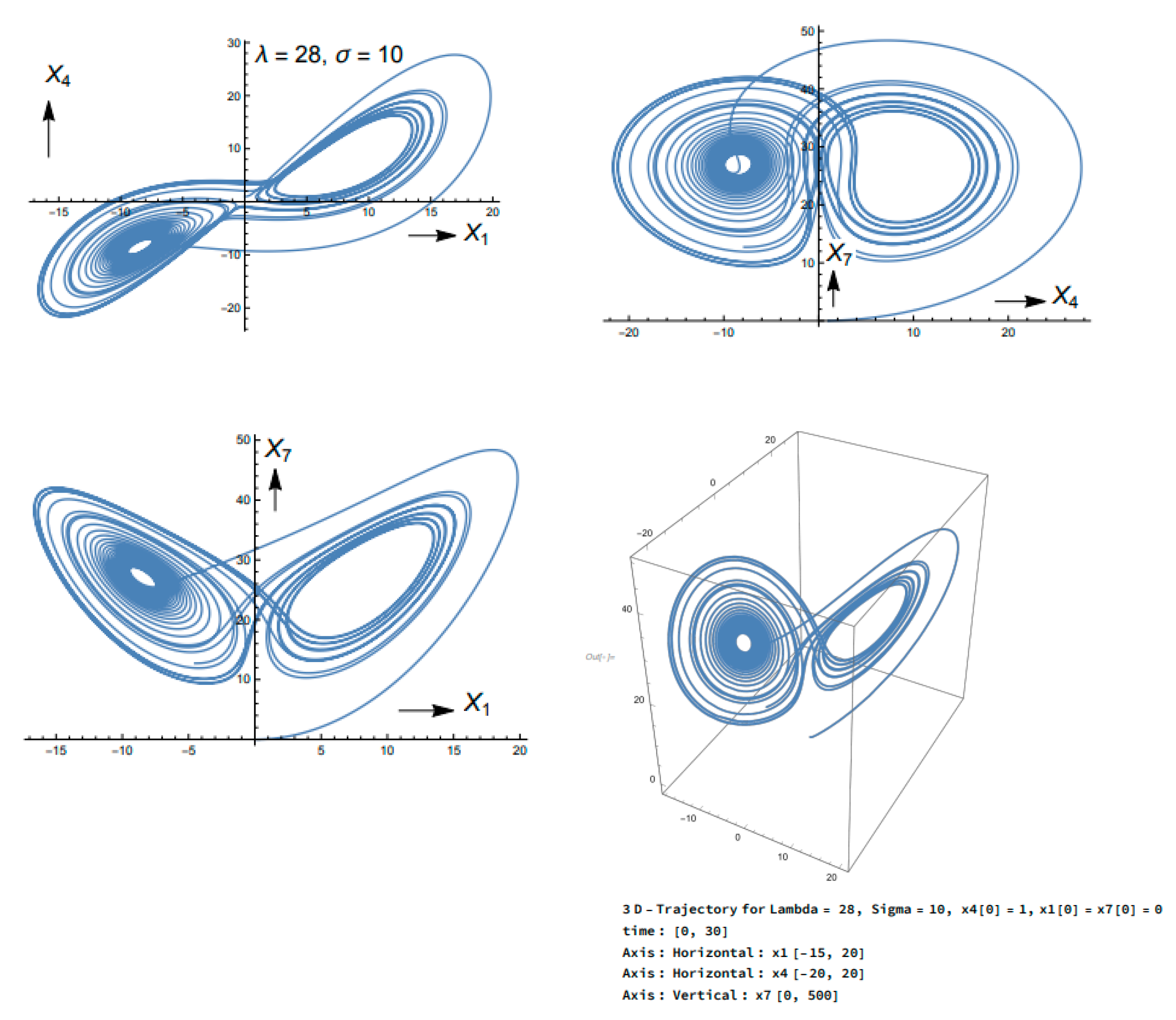
In the first three panels of Figure 4, amplitudes are depicted in pairs between t = 0   and   t = 30 : x 1 x 4 , x 4 x 7 , and x 1 x 7 . The well-known butterfly pattern appears for each pair over the time period t = 0   to   t = 30 . The convergence to ( x 1 ,   x 4 ,   x 7 ) : ( 6 2 ,   6 2 ,   27 )   and   (− 6 2 ,   6 2 ,   27 ) does not occur in finite time, only as t . The 3-D phase plot of amplitudes is shown in the lower right corner of Figure 4 where the two steady-state solutions are located at the centroids of the circular/elliptical trajectories.
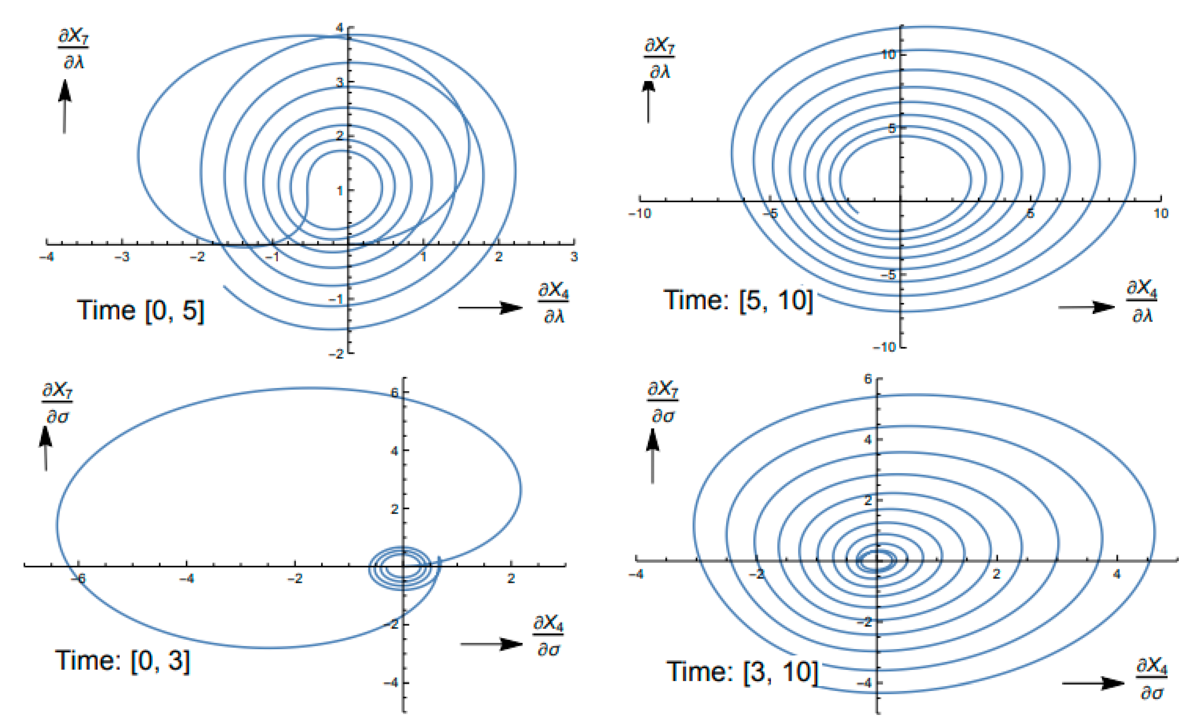
The time evolution of sensitivities   x 7 λ ,   x 7 σ is shown in Figure 5. Here, we have broken the plots into two time zones: t   [ 0 ,   5 ]   and   t   [ 5 ,   10 ] for x 7 λ and t   [ 0 ,   3 ] and t   [ 3 ,   10 ] for x 7 σ . Note that the coordinate axes are scaled differently in these plots. Plots for x 4 λ ,   x 4 σ exhibit similar structures. The common thread between sensitivity plots is that the magnitudes oscillate between + and − values and increase ad infinitum.
The sensitivity of the x 1 ( t ) solution to a small change in the initial condition is shown in Figure 6. In this figure, a 5% change in the initial condition leads to significant change in x 1 ( t ) after t ~ 20.

4. Design of Observation Network

4.1. Model and Forecast Sensitivities

Let X ( k ) = ( x 1 ( k ) ,   x 4 ( k ) ,   x 7 ( k ) )   ϵ R 3 be the state of the S-LOM (3) or L-LOM (3) model at times k = 0 ,   1 ,   2 ,   3   given by
X ( k + 1 ) = M ( X ( k ) , α )   ϵ   R 3
with X ( 0 )   ϵ R 3 as initial condition, α = ( α 1 ,   α 2 ) = ( λ ,   σ ) T ϵ   R 2 , the parameter vector, and X ( k ) = X ( k , X ( 0 ) , α ) the solution.
Define forecast sensitivity to parameters as
V ( k ) = X ( k ) α   ϵ   R 3 x 2 = [ x 1 λ x 1 σ x 4 λ x 4 σ x 7 λ x 7 σ ]
It can be shown that V ( k )   evolves according to the discrete time dynamics given by
V ( k + 1 ) = D M ( k ) V ( k ) + D M α ( k ) w i t h   V ( 0 ) = 0
where
D M ( k ) = x j ( 0 ) [ M i ( X ( k ) ,   α ) ]   ϵ   R 3 x 3
D M α ( k ) = α j [ M i ( X ( k ) ,   α ) ]   ϵ   R 3 x 2
with α = ( α 1 ,   α 2 ) = ( λ   ,   σ   ) [15,16].
An example of forecast sensitivity to parameter λ has been shown earlier in Equation (15).

4.2. Forecast Error

Let c ¯ = α ¯ be the true control and X ¯ ( k ) be the solution starting from c ¯ . Let c = α be the arbitrary control and let X ( k ) be the model solution starting from c .
Define
δ c = c ¯ c = δ α = α ¯ α
where α ¯ α = ( λ ¯ λ ,   σ ¯ σ ) T = [ δ λ δ σ ] = δ α .
Let δ X ( k ) be the change in the state X ( k ) resulting from change δ c . Then, from Equation (19) and using first-order Taylor expansion, we obtain
δ X ( k ) = X ¯ ( k ) X ( k ) = X ( k ,   X ( 0 ) ,   α ¯ ) X ( k ,   X ( 0 ) , α ) = X ( k ) α δ α = V ( k ) δ α

4.3. Observations and Cost Function

We work with L-LOM (3) in this subsection.
Consider the physical domain defined by the rectangle
D = { η = ( x ,   z ) T } ,         0 x 6 2 ,       0 z 1
where x denotes the lengthwise coordinate and z the breadthwise coordinate of a point η in D . Convection is confined to this domain.
Define a matrix
H ( η ) = [ f 4 ( η ) ,   f 7 ( η ) ] ϵ   R 1 x 2
where
f 4 ( η ) = cos ( π a x ) sin ( π z ) f 7 ( η ) = sin ( 2 π z )
Let
θ ¯ ( k , η ) = H ( η ) [ x ¯ 4 x ¯ 7 ] = H ( η ) X ¯ ^ + ξ ( k )
be the actual observation where X ¯ ^ is the projection of X ¯ onto its last two elements and ξ ( k )   is the observation noise with variance σ 2 .
Let
θ M ( k ,   η ) = H ( η ) [ x 4 x 7 ] = H ( η ) X ^
where θ M ( k , η ) is the model counterpart to the observation based on perturbed control.
The difference is called the forecast error or innovation (innov).
e ( k ) = θ ¯ ( k , η ) θ M ( k ,   η )
Using Equations (28) and (29), we rewrite Equation (30) as
e ( k ) = H ( η ) ( X ¯ ^ X ^ ) = H ( η ) δ X ^
For α   ϵ   R 2 and η   ϵ   R 2 , we define the cost function for a given ( k ,   η ) as
J ( α , k ,   η ) = 1 2 σ 2 ( θ ¯ ( k , η ) θ M ( k ,   η ) ) 2
The squared difference between the observation θ ¯ ( k , η ) and its model counterpart θ M ( k ,   η ) . This cost function in Equation (32) is additive in the number of observations. Using Equations (31) and (32), we get
J ( α ,   η ) = 1 2 σ 2 ( H ( η ) ( δ X ^ ) T H ( η ) ( δ X ^ ) = 1 2 σ 2 ( δ X ^ ) T H T ( η ) H ( η )   ( δ X ^ )
Using first-order Taylor expansion, the vector of temperature departure error components, [ δ x 4 δ x 7 ] , can be represented by
δ X ^ = [ δ x 4 δ x 7 ] = [ x 4 ( k ) λ x 4 ( k ) σ x 7 ( k ) λ x 7 ( k ) σ ] [ δ λ δ σ ] = V ^ ( k ) δ α ,
where V ^   ( k ) is a submatrix of the forecast sensitivity matrix V ( k ) ;   namely, the last two rows of that matrix. Arguments related to the derivation of Equation (34) are found in Lakshmivarahan et al. [7].
Substituting Equation (34) into Equation (33), we get
J ( α ,   η ) = 1 2 σ 2 ( δ α ) T [ V ^ T ( k )   (   H T ( η ) H ( η ) ) V ^ ( k ) ] δ α = 1 2 σ 2 ( δ α ) T G   ( δ α ) = 1 2 σ 2 ( δ α ) T G   ( δ α )
where
G ( k ) V ^ T ( k )   (   H T ( η ) H ( η ) ) V ^ ( k ) ] = V ^ T ( k ) H ¯ ( η ) V ^ ( k ) ]
and
H ¯ ( η ) H T ( η ) H ( η )
Remark 1.
It is important to note that G ( k ) applies to a single time k . Since the cost function is additive in the number of observations, i.e., if there is more than one observation, a separate matrix exists for each time. Take the case when observations are available at three observation times with G   matrices G 1 ,   G 2 ,   and   G 3 , then the appropriate combined matrix will be G = G 1 + G 2 + G 3 .
In the presence of two forms of the cost function, namely Equation (32) and (35), we use Equation (35) to determine observation placement. We use Equation (32) to display the structure of the cost function in the space of controls.
From Equation (35), the gradient of J ( α ,   η ) , J ( α , η ) , is given by
J ( α , η ) = [ J λ J σ ] = G   ( δ α )
To determine the optimal adjustment to control through FSM, we write the cost function as
J ( α , η ) = 1 2 σ 2 ( H X ^ + H ( η ) X ^ α δ α θ ¯ ) T ( H X ^ + H ( η ) X ^ α δ α θ ¯ )
where
H ( η ) X ^ α = H ( η )   V ^
Expanding Equation (40) and setting its gradient to zero yields
δ α = ( G T G ) 1 G T i n n o v
where the innovation i n n o v is given by
i n n o v = H X ^ θ ¯

4.4. Observation Placement

In this paper we consider two structures for the observations: (1) time only, and (2) time and space. Our strategy for observation placement is to render G positive definite. However, not only render it positive definite, but also reduce its condition number so that a “bowl-like” cost function’s structure is present in the vicinity of its true minimum located at α ¯ = ( λ ¯ ,   σ ¯ ) for error-free observations. Two types of observations are considered: (a) observations in time alone (Section 4.4.1) and (b) observations in space and time (Section 4.4.2).

4.4.1. Observations in Time Alone

When we consider observations of spectral components X ¯ ( k ) as a function of time alone in our data assimilation problem, the H   ( η ) matrices in Equation (36) are replaced by identity matrices and the cost function then becomes
J ( α ) = 1 2 σ 2 ( δ α ) T [ V ^ T ( k )   V ^ ( k ) ] δ α
where G = V ^ T ( k ) V ^ ( k ) is positive definite as shown below. In matrix form
V ^ T ( k ) V ^ ( k ) = [ ( x 4 ( k ) λ ) 2 + ( x 7 ( k ) λ ) 2 ( x 4 ( k ) λ x 4 ( k ) σ + x 7 ( k ) λ x 7 ( k ) σ ) ( x 4 ( k ) λ x 4 ( k ) σ + x 7 ( k ) λ x 7 ( k ) σ ) ( x 4 ( k ) σ ) 2 + ( x 7 ( k ) σ ) 2 ]
or alternatively represented by
V ^ ( k ) = ( ε 1 ( k ) ,   ε 2 ( k ) )                     V ^ T = [ ε 1 T ( k ) ε 2 T ( k ) ]
V ^ T ( k ) V ^ ( k ) = [ ε 1 T ( k ) ε 1 ( k ) ε 1 T ( k ) ε 2 ( k ) ε 2 T ( k ) ε 1 ( k ) ε 2 T ( k ) ε 2 ( k ) ]
From this point onwards, we simplify notation by omitting the parenthetical expression “ ( k ) ” following forecast sensitivities.
From the physics of our problem, V ( k ) is sensitive to λ   and   σ .   The dot products “ a ,   b ” are expressed in matrix-vector notation where ε 1 ( k ) and ε 2 ( k ) are the first and second columns of V ^ ( k ) .
ε 1 ,   ε 2 = ε 1 T ε 2 = ε 2 T ε 1 = ε 2 ,   ε 1  
ε 1 T ,   ε 1 = ε 1 2 ,   ε 2 T ,   ε 2 = ε 2 2
Thus,
V ^ T ( k ) V ^ ( k ) = [ ε 1 2 ε 1 ,   ε 2 ε 2 ,   ε 1 ε 2 2 ]
Further, ε 1 2 > 0 and ε 2 2 > 0 , and the determinant of V ^ T ( k ) V ^ ( k ) is given by
det   ( V ^ T V ^ ) = ε 1 2   ε 2 2 < ε 1 ,   ε 2 > 2  
and
ε 1 ,   ε 2 = ε 1   ε 2 cos θ
so
< ε 1 ,   ε 2 > 2 = ε 1 2 ε 2 2   cos 2 θ
The determinant of V ^ T V ^ can then be written as
det   ( V ^ T V ^ ) = ε 1 2 ε 2 2 ε 1 2 ε 2 2   cos 2 ( θ ) = ε 1 2 ε 2 2 ( 1 cos 2 θ ) > 0   ( i f   θ 0 )
So long as ε 1   and   ε 2 are not colinear or θ = 0   or   180 ° ,   then
cos θ 0 ,   and det ( V ^ T V ^ ) > 0
and the following inequalities hold
ε 1 2 > 0 ,   ε 2 2 > 0 ,     and   det ( V ^ T V ^ ) > 0
These inequalities imply that V ^ T V ^ is a positive definite matrix.
The strategy for choosing observations is therefore:
Pick observation z ( k ) = X ^ ( k ) + υ ( k ) when z ( k )   ϵ   R 2 and noise υ ( k )   ϵ   R 2 such that z ( k 1 ) at time k 1 makes ε 1 2 a maximum and z ( k 2 ) makes ε 2 2 a maximum.
Then, at
k 1 : V ( k 1 ) = [ ε 1 ( k 1 ) ,   ε 2 ( k 1 ) ]
and at
k 2 : V ( k 2 ) = [ ε 1 ( k 2 ) ,   ε 2 ( k 2 ) ]
and
G = V T ( k 1 ) V ( k 1 ) + V T ( k 2 ) V ( k 2 ) = G ( k 1 ) + G ( k 2 )  

4.4.2. Observations Taken in Space and Time

When observation locations are to be determined in space and time, the G matrix takes the form
G ( k , η ) = V ^ T ( k )   (   H T ( η ) H ( η ) ) V ^ ( k ) ] = V ^ T ( k ) H ¯ ( η ) V ^ ( k ) ] .
The space element H ¯ ( η ) is separable from the time elements V ^ T ( k ) and V ^ T ( k )   or in combination V ^ T ( k )   V ^ ( k ) . In the presence of this separability, the strategy reduces to first determining desired times as explained above. This is followed by determining desired positions in ( x ,   z ) space.
Recall that x ^ = ( x 4 ,   x 7 ) T and α = ( λ ,   σ ) T and represent V ^ as a column partition
V ^ = [ x 4 λ x 4 σ x 7 λ x 7 σ ] = [ x ^ λ ,   x ^ σ   ] = [ V 1 ,   V 2 ]  
Define vectors
g 4 = [ x 4 α ] = ( x 4 λ ,   x 4 σ ) T   ϵ   R 2
and
g 7 = [ x 7 α ] = ( x 7 λ ,   x 7 σ ) T   ϵ   R 2  
It can be verified that the row partition of V ^ is given by
V ^ = [ g 4 T g 7 T ]
Recall that H is given by
H = [ f 4 ,   f 7 ]   ϵ   R 1 x 2
where f 4 = cos ( π a x ) sin ( π z ) and f 7 = sin ( 2 π z ) .
Using Equations (60) and (61), we obtain a row vector w ( k ,   η ) = ( w 1 ( k ,   η ) ,   w 2 ( k ,   η ) ) given by
w ( k ,   η ) = H V ^ = [ f 4 ,   f 7 ] [ g 4 T g 7 T ] = ( f 4 g 4 T + f 7 g 7 T )   ϵ   R 1 x 2
Consequently, we can express the Gramian G ( k ,   η ) as a rank-one symmetric product matrix
G ( k ,   η ) = w T ( k ,   η ) w ( k , η ) = [ w 1 2 ( k ,   η ) w 1 ( k ,   η ) w 2 ( k ,   η ) w 2 ( k ,   η ) w 1 ( k ,   η ) w 2 2 ( k ,   η ) ]
Strategy for determining observation placement:
(1)
Pick η ( x ,   z ) such that f 4 and f 7 are maximum
(2)
Let k 1 ,   k 2 ,   k 3 ,   k 4 be four time instances where the squares of x 4 λ ,   x 4 σ ,   x 7 λ ,   x 7 σ are maximum. Determine the respective G ( k i ,   η ) ’s. Then, the final Gramian is given by
G = G ( k 1 , η ) + G ( k 2 , η ) + G ( k 3 , η ) + G ( k 4 , η )  
Remark 2.
In principle we can use just two observations at times k 1 and k 2 where ( x 4 λ ) 2 and ( x 7 σ ) 2 attain their maxima.

5. Data Assimilation Experiments

Once the observations and their locations have been determined, the FSM method of data assimilation is used to determine optimal values of controls. Development of the FSM was first shown in Lakshmivarahan and Lewis [15] and explored with numerous examples in the textbook Lakshmivarahan et al. [16]. In our case, the optimal values of control are found through the iterative methodology captured by Equation (41). Starting from guess control, solution to Equation (41) delivers the adjustment to guess control. The adjustment is added to the guess and the second operating point in space of control is determined. New forecasts and new forecast sensitivities are found from the updated controls. The process continues until the cost function’s change falls within a specified tolerance.

5.1. Experiment I: Nonchaotic Data Assimilation Process (Lorenz Scaling)

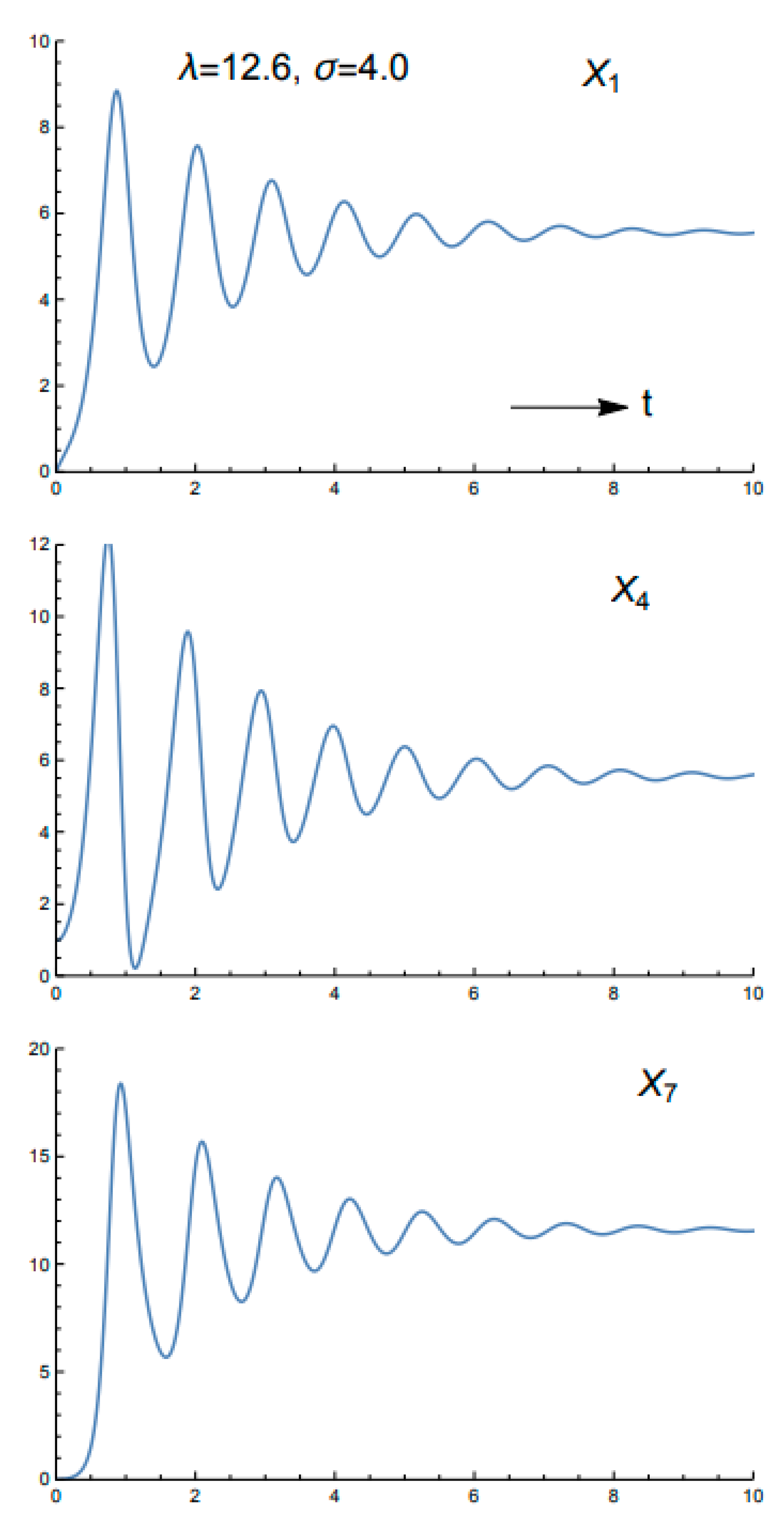
True controls are taken to be λ = 12.0 ,   σ = 7.0 . The forecasts of x 1 ,   x 4 ,   x 7 based on guess control ( λ = 12.6 ,   σ = 4.0 ) are shown in Figure 7. The amplitudes reach steady state near t = 10. Graphs of the diagonal elements of V T V that dictate observations to be made at t = 1 are shown in Figure 8. The observations at this time are found by adding 10 % random error to the forecast based on true controls. The observations of x 4 ( O b x 4 ) and x 7 ( O b x 7 ) at t = 1 are given by
( O b x 4 ,   O b x 7 ) = ( 0.371 ,   11.378 ) .
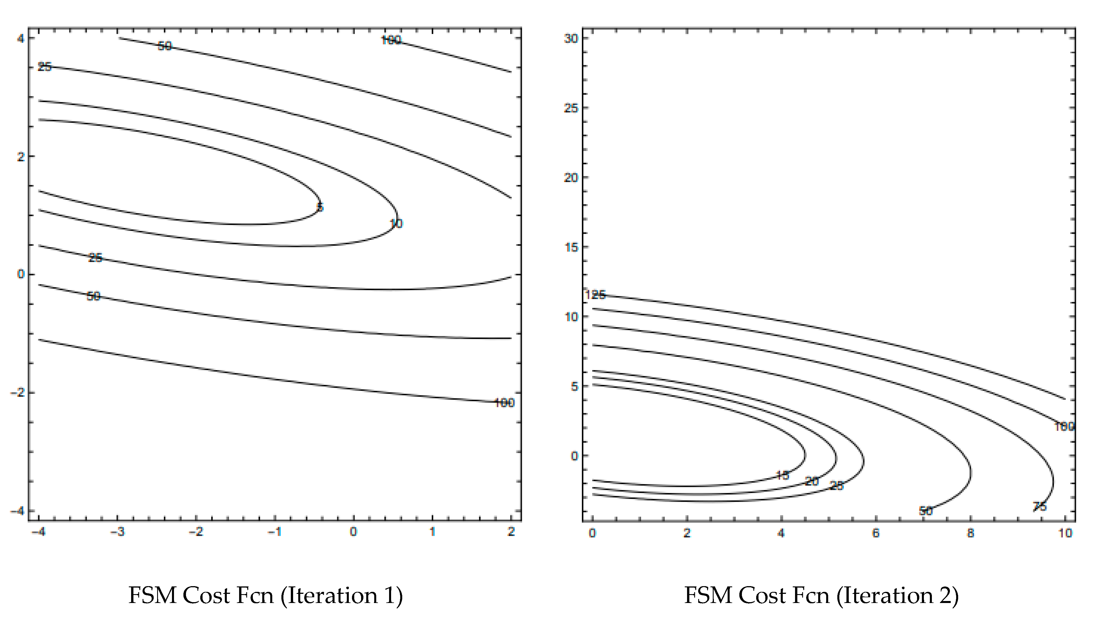
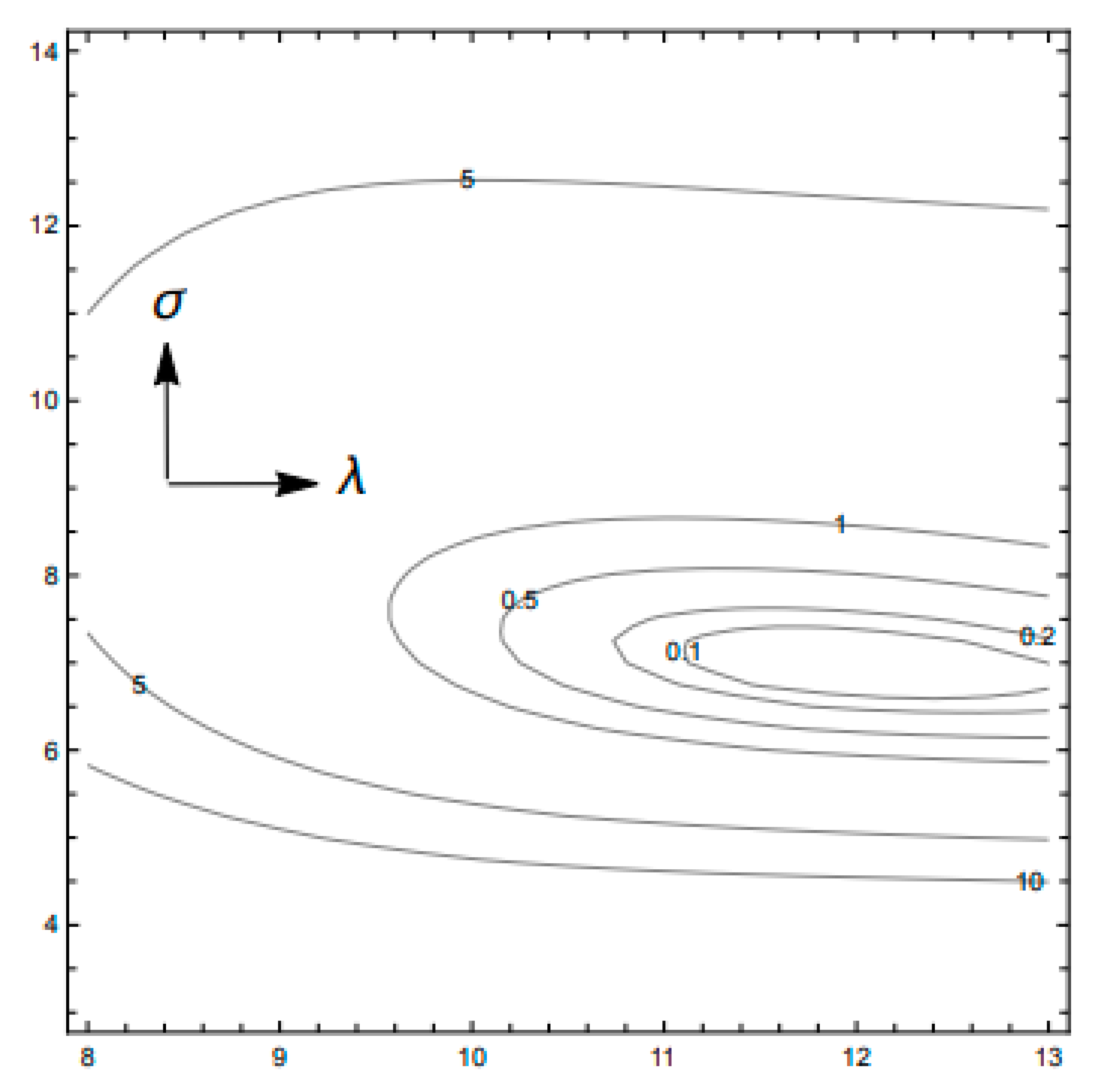
Table 2 summarizes results from FSM. The assimilation process converges to a solution in 4 steps. The last column of Table 2 displays the sequential reduction in cost function values from ~19 to 3 · 10 5 , reduction by a factor of 10 6 . FSM determines values of λ   and   σ at each of the 4 iterations. The plot of these values is shown in Figure 9. The contours are always elliptical since the FSM cost function at each iteration is quadradic in λ   and   σ . Display of cost function Equation (32) is shown in Figure 10 and the minimum is found to be located at λ = 12 ,   σ = 7 .
In a test that changed observation time from t o b s = 1.00 to t = 1.05, the data assimilation algorithm converged to ( λ ,   σ ) = ( 11.995 ,   6.968 ) in 4 iterations.

5.2. Experiment II: Nonchaotic Data Assimilation Process (Saltzman Scaling)

This data assimilation experiment follows the exact steps for the nonchaotic data assimilation process as shown in Section 5.1 except that the governing 3-mode equations are scaled according to Saltzman’s form of the equations as found in Equations (3)–(5).
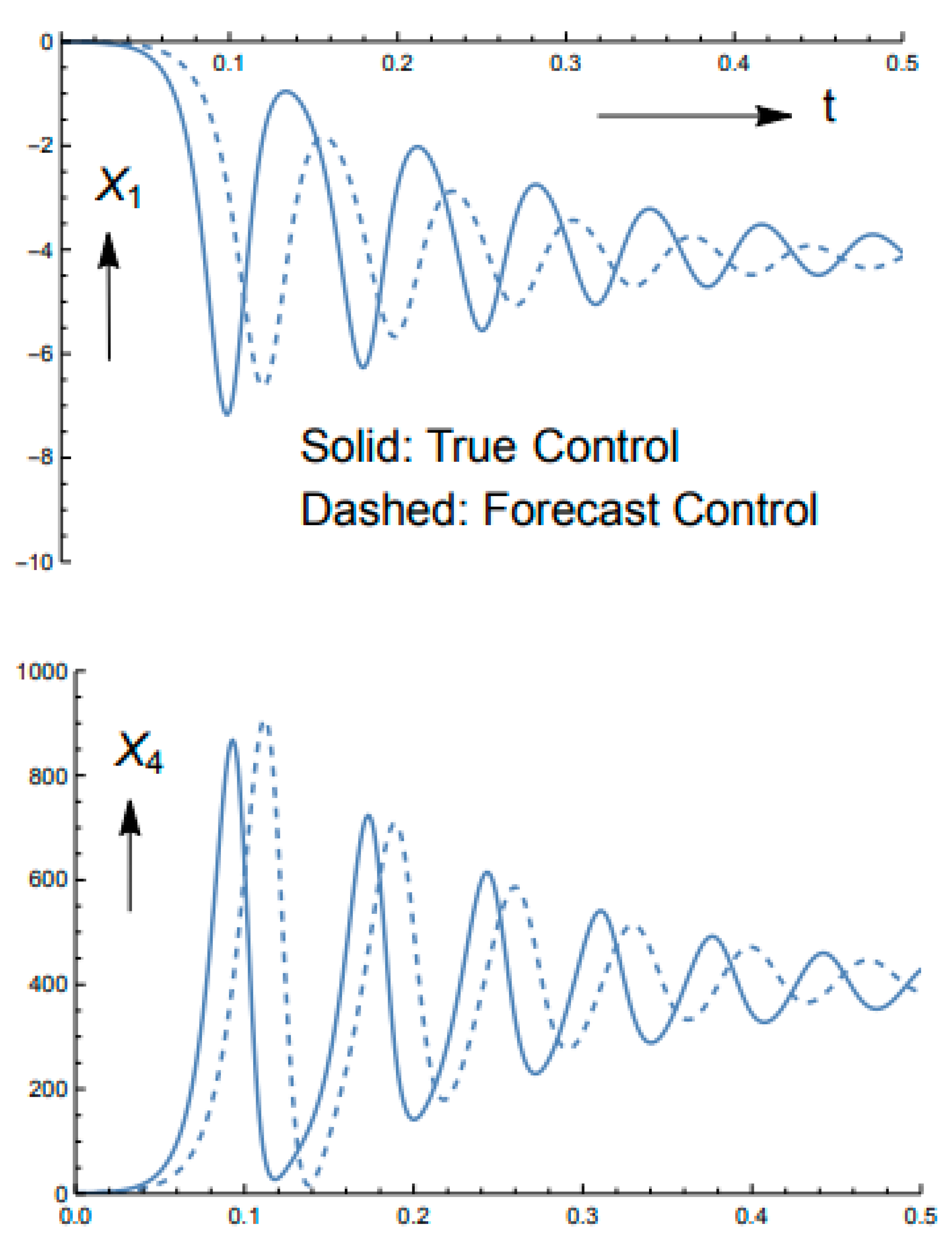
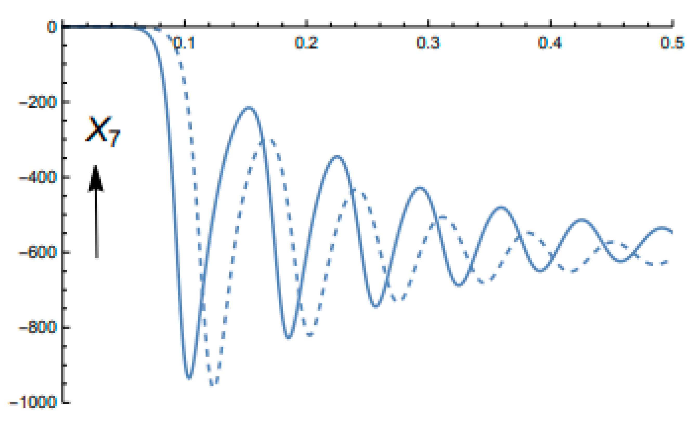
Figure 11 displays the time-dependent solutions to the 3-mode model. The solid curves are derived from the true controls ( λ = 12 ,   σ = 7 ) and the dashed curves from forecast controls ( 12.6 ,   4.0 ) .   The primary difference between this forecast and the one shown earlier for Lorenz’s scaling is the much greater magnitudes of the variables and the shorter time required to reach equilibrium. Otherwise, the time-dependent oscillatory nature of the components is the same. The forecast sensitivity of x 4 and x 7 to λ   and   σ are shown in Figure 12—again the sensitivities are much greater than those associated with Lorenz’s scaling. Based on the elements of the sensitivity product matrix V T V , t o b s = 0.16. The observations at this time are found by adding 10 % random error to the forecast based on true controls. The observations of x 4 ( O b x 4 ) and x 7 ( O b x 7 ) at t = 0.16 are given by
( O b x 4 ,   O b x 7 ) = ( 427.5 260.6 )
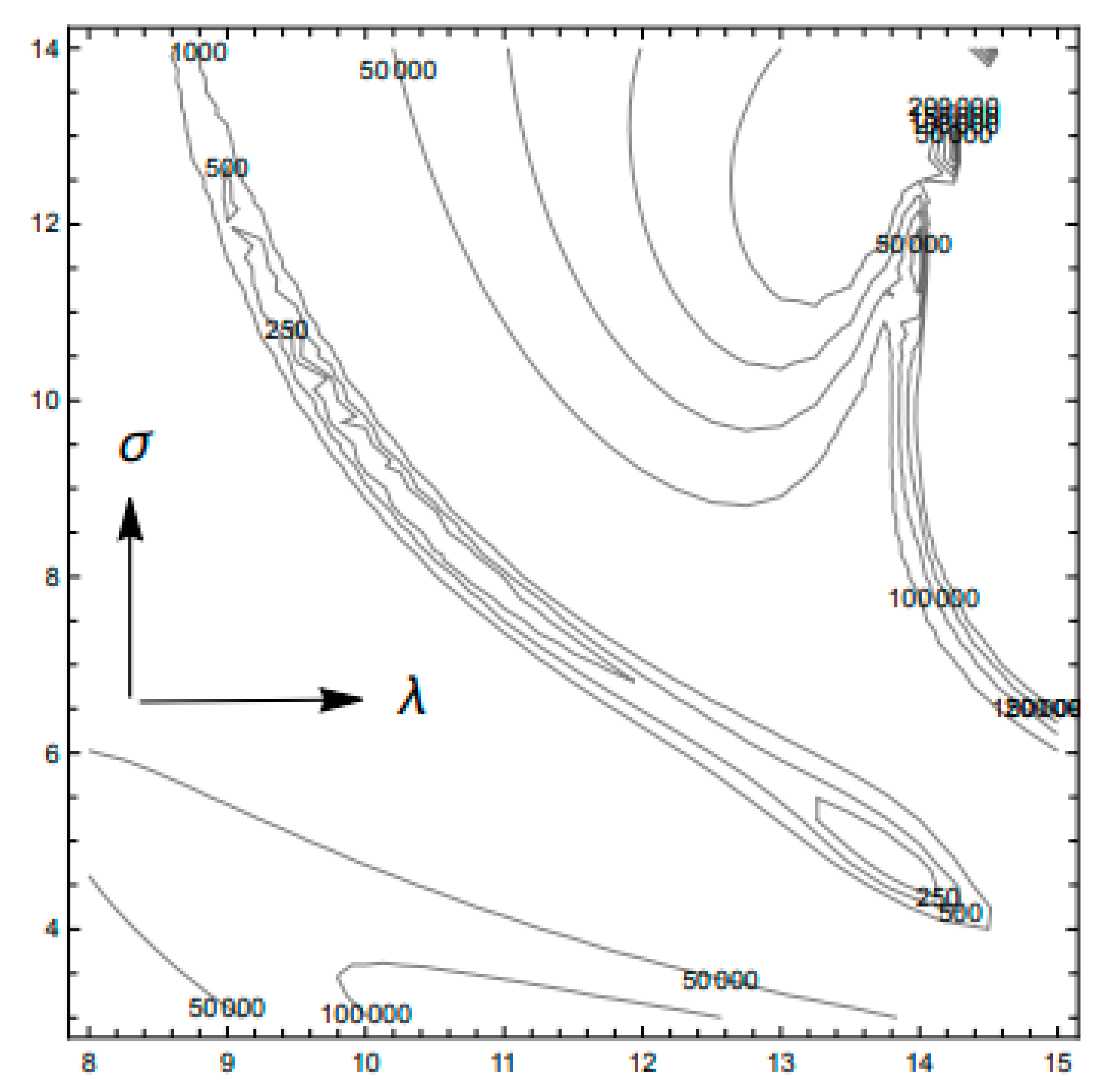
Results from the data assimilation experiment are shown in Table 3. The data assimilation process converges to ( λ ,   σ ) = ( 13.8 ,   4.8 ) in 4 iterations. The cost function is reduced 9 orders of magnitude. The cost function for this case is shown in Figure 13. The converged values of control shown in Table 3 are consistent with this cost function’s minimum.
In a test that changed observation time from t o b s = 0.16 to t = 0.10, FSM did not converge to an optimal state. Instead, after a single iteration the result was ( λ ,   σ ) = ( 46.3 ,   26.8 ) , unreasonable physically.

5.3. Experiment III: Chaotic Data Assimilation Process (Lorenz Scaling)

True controls are taken to be λ = 28.0 ,   σ = 10.0 . The forecasts of x 1 ,   x 4 ,   x 7 based on guess control ( λ = 29.0 ,   σ = 8.0 ) are shown in Figure 14. Based on the elements of the product sensitivity matrix V T · V , observations are collected at t = 0.4 . The observations at this time are found by adding 10 % random error to the forecast based on true controls. The observations of x 4 ( O b x 4 ) and x 7 ( O b x 7 ) at t = 0.4 are given by
( O b x 4 ,   O b x 7 ) = ( 22.832 ,   40.194 ) .  
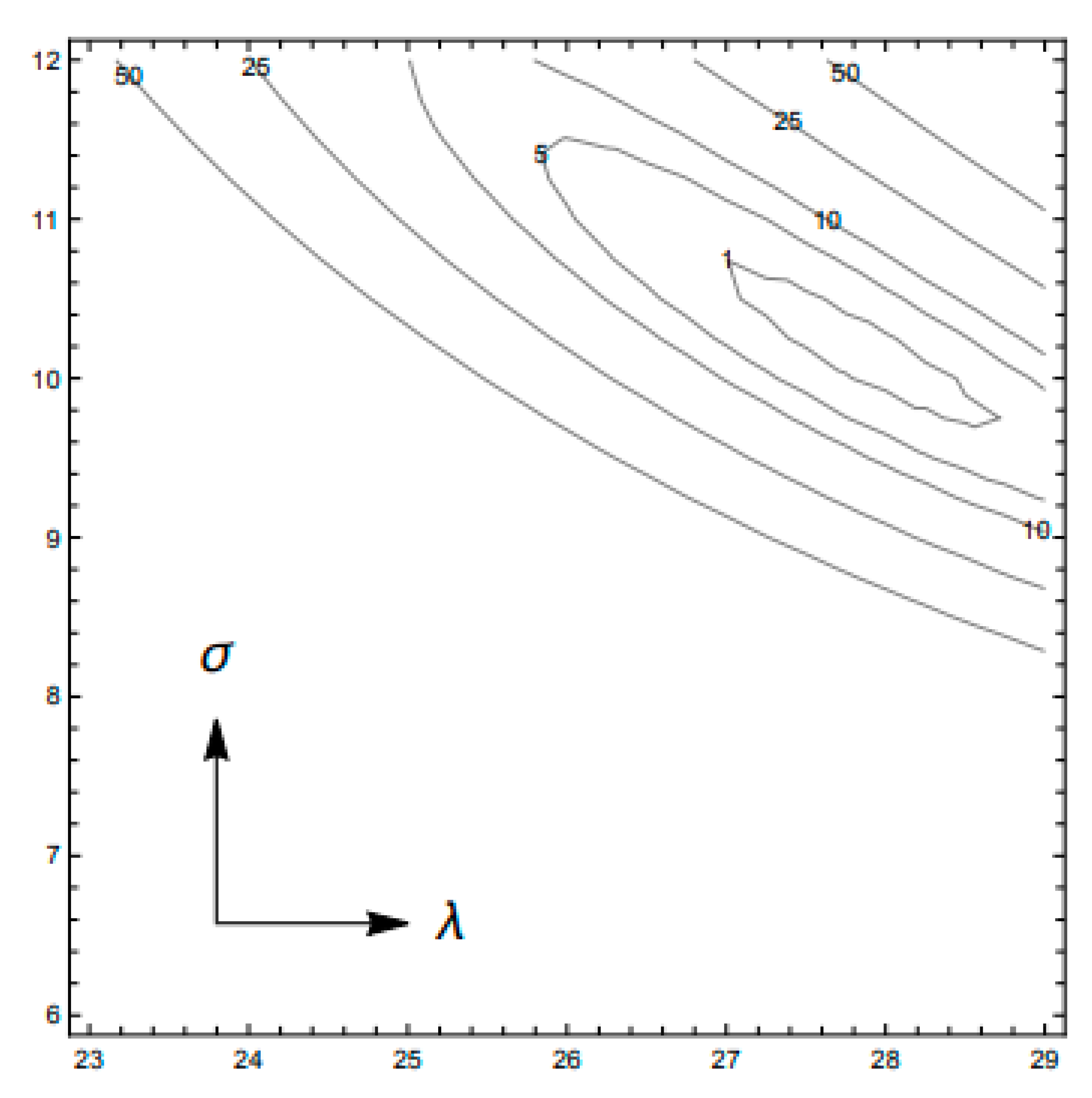
Table 4 summarizes results from FSM. Assimilation process converges to a solution in 4 steps. The last column of the table displays the sequential reduction in cost function values from ~74 to ~ 10 4 , reduction by a factor of 10 6 . The cost function is shown in Figure 15 and the minimum is found to be located at λ = 28 ,   σ = 10 ,   nearly identical to the solution found by FSM.
It is interesting to consider cases where the optimal observation time was greater than t = 0.4, times where the model forecast sensitivities are extremely large as shown earlier in Figure 5. There is no reason to believe that observations at these times would not give a reasonable result. The reasonableness of the result, however, would be dependent on the smallness of the condition number.

5.4. Experiment IV: Data Assimilation in Time and Space (x, z)

We confine our attention to a single numerical experiment that combines space and time. Our experiment focuses on true controls λ = 2   and   σ = 7 , a nonchaotic regime. The perturbed controls are λ = 2.5   and   σ = 3.0 . The time of observation is determined from the structure of the sensitivity product matrix V T V . Based on the trace of V T V , observations are taken at t o b s = 2. The spatial observation sites are determined from the trace of H T H at t = 2. These spatial locations are
x 1 = 0.10     z 1 = 0.25 x 2 = 0.10     z 2 = 0.75 x 3 = 2.55     z 3 = 0.23 x 4 = 3.11     z 4 = 0.68
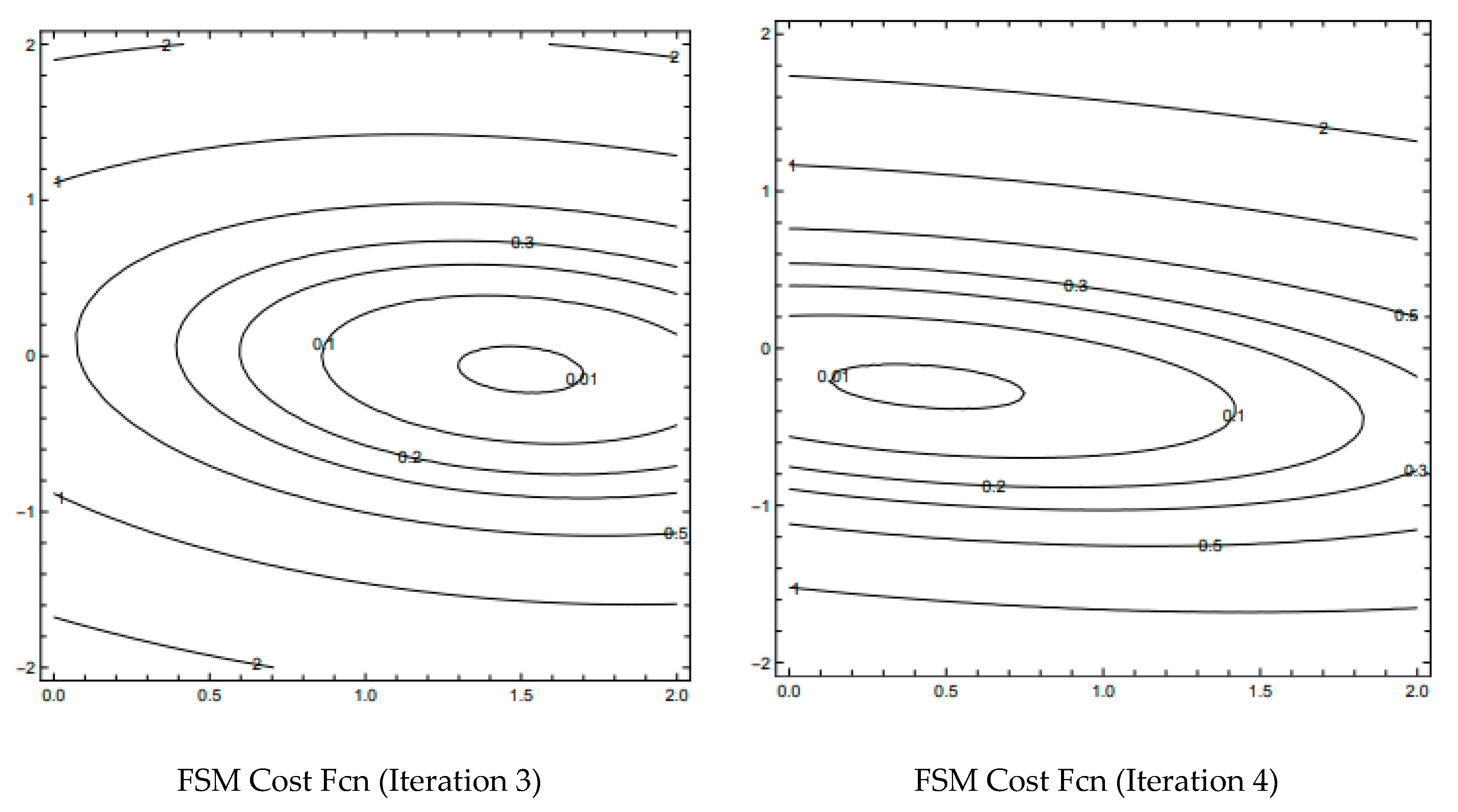
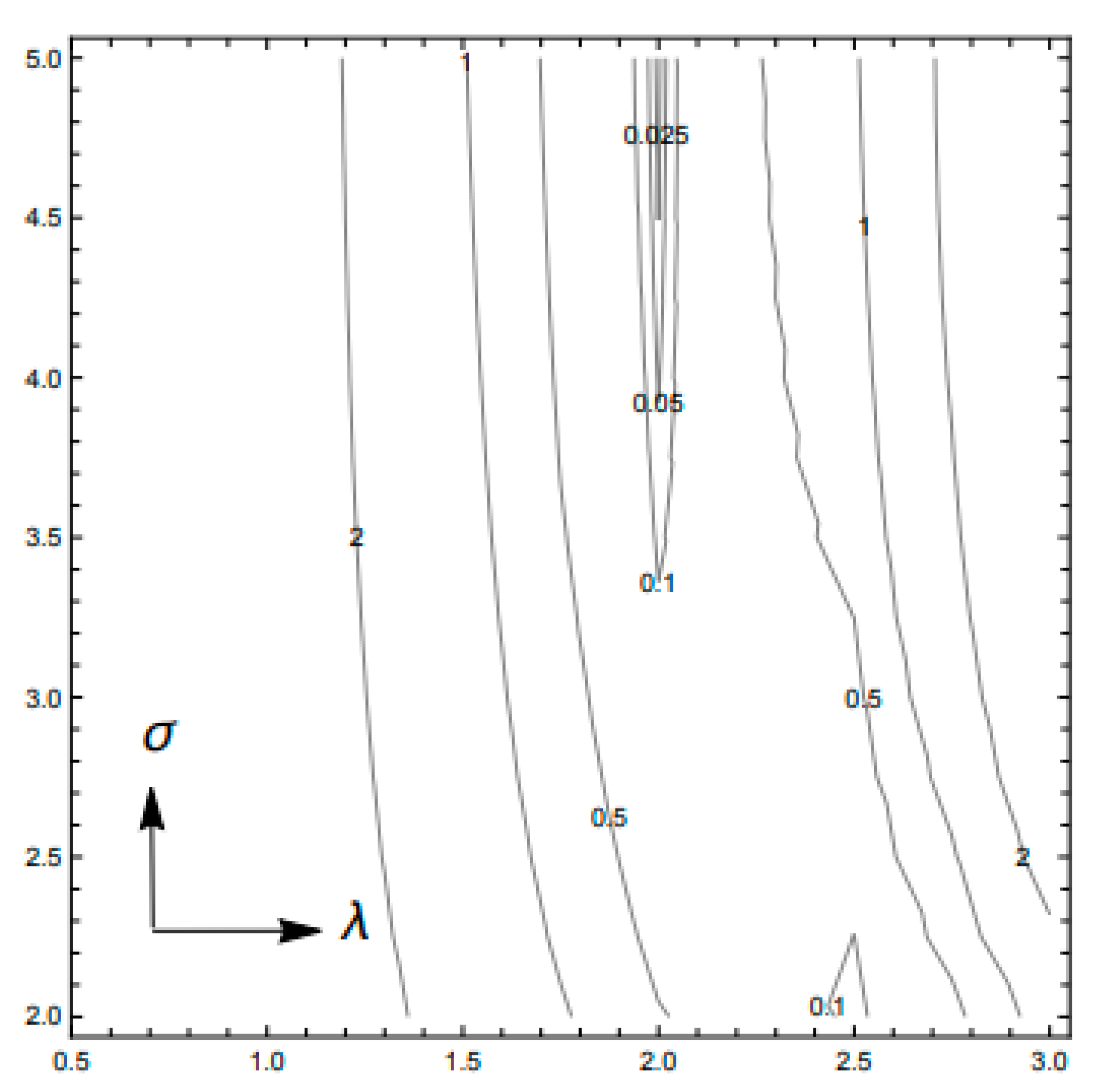
In this case, the condition number for the G matrix is 3.8 which builds convexity into the cost function as shown in Figure 16.
Table 5 summarizes to convergence to optimal solution. The innovations at the observation locations exhibit a reduction of 10 7 in the 3 iterations and the optimal minimum is very close to the minimum shown in Figure 16.

6. Discussion and Conclusions

S-LOM (3) and L-LOM (3), low-order forms of spectral equations that govern Rayleigh–Bénard convection developed by Saltzman [1] and used by Lorenz [4], respectively, have been used to study advantages of observation placement in dynamic data assimilation. Observation placement is controlled by forecast sensitivity to model control; in this case the control has two elements, Rayleigh and Prandtl numbers. We have used FSM data assimilation since it delivers forecast sensitivities to control that are used to determine observation placement.
By examination of the cost function in terms of forecast sensitivities, a Gramian matrix G becomes the centerpiece to determine observation placement. For time-only observations, the Gramian matrix reduces to the product of V T V where V is the time-dependent forecast sensitivity to control. This matrix is symmetric positive definite and the maximum values of the trace or norm of this matrix determine the best observation locations. Observation locations that yield the matrix’s smallest condition number build convexity into the cost function’s minimum. For our case study, the contours of the cost function in the space of the two controls are ellipses. As the condition number approaches the number 1, the major and minor axes of the ellipses approach the same number and the ellipses approach circles. In this case, the path to the minimum is along a straight line. For time-space observations, the Gramian matrix is symmetric semi positive definite in the form V T H T H V where H is the spatial-dependent matrix that accounts for the double Fourier series representation of the observations. This product exhibits separability in space and time and therefore permits determination of observation-time placement as a first step to be followed by spatial placement of observations.
We tested the observation placement strategy for both nonchaotic and chaotic regimes. Results from the numerical experiments with FSM were especially good based on (1) iterative reduction of the cost functions’ values, and (2) comparison of the optimal parameters with the cost function minimum in the space of controls.
We also wanted to test the role of equation scaling in the data assimilation process. The two models have different scaling where S-LOM (3) follows the standard fluid dynamical scaling based on the fluid’s physical parameters while L-LOM (3) incorporates various forms of the non-dimensional wavenumber along with the physical parameters in its scaling. The scaling for L-LOM (3) leads to coefficients of comparable magnitude in the governing amplitude differential equations while scaling for S-LOM (3) leads to order of magnitude differences in the coefficients. In turn, the forecast sensitivity equations for S-LOM (3) exhibit large differences in their coefficients. Nevertheless, the FSM data assimilation method delivered good results for both models. On the other hand, when the ideal observation time is changed slightly, S-LOM (3) results were poor while L-LOM (3) were excellent. It thus appears that scaling plays an important role in data assimilation, at least for our limited number of experiments.

Author Contributions

Formal analysis, J.M.L. and S.L.; Writing—original draft, J.M.L. and S.L.; Writing—review & editing, J.M.L. and S.L. All authors have read and agreed to the published version of the manuscript.

Funding

This research received no external funding.

Institutional Review Board Statement

Not applicable.

Informed Consent Statement

Not applicable.

Acknowledgments

We thank Bo-Wen Shen for encouraging us to explore application of FSM to chaotic systems. The authors also thank: (1) Kevin Fisher-Mack and Junjun Hu for writing the computer program that delivered the cost function display in the space of controls, and (2) the three anonymous reviewers who made cogent suggestions that were followed and this led to clarification of discussions in the paper.

Conflicts of Interest

The authors declare no conflict of interest.

References

  1. Saltzman, B. Finite Amplitude Free Convection as an Initial Value Problem-I. J. Atmos. Sci. 1962, 19, 329–341. [Google Scholar] [CrossRef]
  2. Bénard, M. Les Tourbillions cellulaires dans une nape liquide. Rev. Générale Des Sci. Pures Et Appl. 1990, 11, 1261–1271, 1309–1328. [Google Scholar]
  3. Rayleigh, L. Convection currents in a horizontal layer of fluid, when higher temperature is on the underside. Philos. Mag. 1916, 32, 529–546. [Google Scholar] [CrossRef] [Green Version]
  4. Lorenz, E.N. Deterministic Nonperiodic Flow. J. Atmos. Sci. 1963, 20, 220–241. [Google Scholar] [CrossRef]
  5. Saravanan, R. The Climate Demon: Past, Present, and Future of Climate Change; Cambridge University Press: Cambridge, UK, 2022; 379p. [Google Scholar]
  6. Lewis, J.M.; Lakshmivarahan, S.; Dhall, S.K. Dynamic Data Assimilation: A Least Squares Approach; Cambridge University Press: Cambridge, UK, 2006; 654p. [Google Scholar]
  7. Lakshmivarahan, S.; Lewis, J.M.; Hu, J. On Controlling the Shape of the Cost Functional in Dynamic Data Assimilation: Guidelines for Placement of Observations and Application to Saltzman’s Model of Convection. J. Atmos. Sci. 2020, 77, 2969–2989. [Google Scholar]
  8. Lakshmivarahan, S.; Lewis, J.M.; Maryada, S.K.R. Observability Gramian and its Role in the Placement of Observations in Dynamic Data Assimilation. In Data Assimilation for Atmospheric, Oceanic and Hydrographic Applications; Park, S.K., Xu, L., Eds.; Springer: Cham, Switzerland, 2022; Volume IV, pp. 215–257. [Google Scholar]
  9. Lewis, J.M.; Lakshmivarahan, S.; Maryada, S.K.R. Placement of observations for variational data assimilation: Application to Burgers’ Equation and seiche phenomenon. In Data Assimilation for Atmospheric, Oceanic and Hydrographic Applications; Park, S.K., Xu, L., Eds.; Springer: Cham, Switzerland, 2022; Volume IV, pp. 215–257. [Google Scholar]
  10. Lakshmivarahan, S.; Lewis, J.M.; Hu, J. Saltzman’s Model: Complete Characterization of Solution Properties. J. Atmos. Sci. 2019, 76, 1587–1608. [Google Scholar] [CrossRef]
  11. Chandrasekhar, S. Hydrodynamic and Hydromagnetic Stability; Oxford at the Clarendon Press: Oxford, UK, 1961; 654p. [Google Scholar]
  12. Turner, J.S. Buoyancy Effects in Fluids; Cambridge University Press: Cambridge, UK, 1973; 368p. [Google Scholar]
  13. Lewis, J.M.; Lakshmivarahan, S. Derivation of Saltzman’s spectral equations for Rayleigh-Bénard convection in terms of two variable parameters, Rayleigh and Prandtl numbers. Tech. Rep. 2019; Unpublished. [Google Scholar]
  14. Kuo, H.-L. Solution of the nonlinear equations of cellular convection and heat transport. J. Fluid Mech. 1961, 10, 611–634. [Google Scholar] [CrossRef]
  15. Lakshmivarahan, S.; Lewis, J.M. Forward Sensitivity Based Approach to Dynamic Data Assimilation. Adv. Meteorol. 2010, 2010, 375615. [Google Scholar] [CrossRef]
  16. Lakshmivarahan, S.; Lewis, J.M.; Jabrzemski, R. Forecast Error Correction Using Dynamic Data Assimilation; Springer: Berlin/Heidelberg, Germany, 2017; 270p. [Google Scholar]
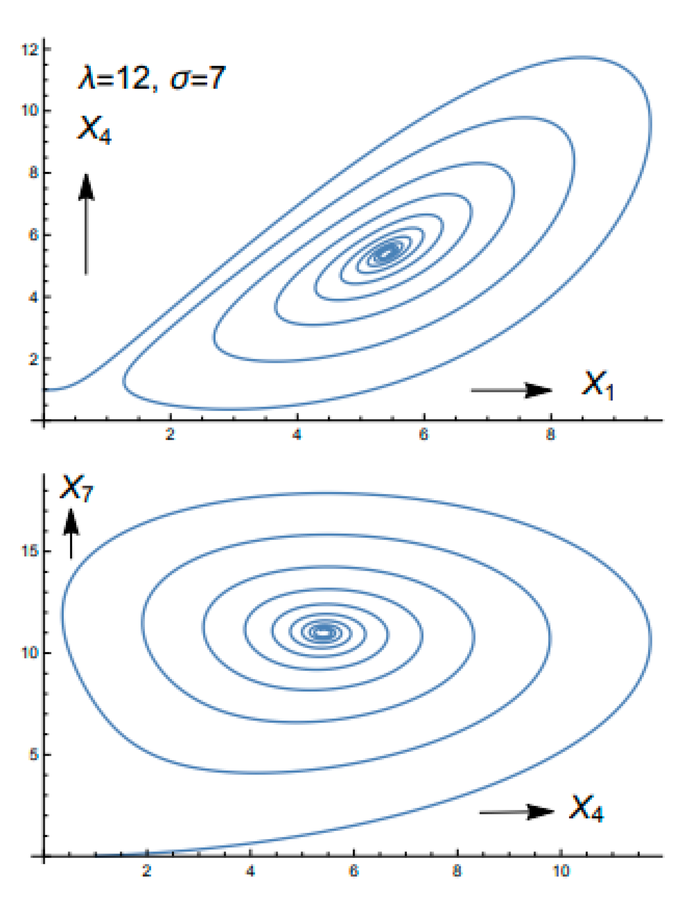
Figure 1. Phase diagrams for the nonchaotic regime with controls λ = 12 ,   σ = 7 over time span [0, 10]: Panel 1 ( x 1 ,   x 4 ) ,   Panel   2   ( x 4 ,   x 7 ) ,   Panel   3   ( x 1 , x 7 ) ,   and Panel 4   ( x 1 , x 4 , x 7 ) with axes: horizontal x 1 [ 0 ,   10 ] ,   x 4 [ 0 ,   12 ] ,   x 7 [ 0 ,   20 ] .
Atmosphere 13 01647 g001aAtmosphere 13 01647 g001b
Figure 2. Forecast sensitivities of x 4 and x 7 with respect to ( λ , σ ) over time span [0, 14] for the non-chaotic regime with controls λ = 12 ,   σ = 7 .
Atmosphere 13 01647 g002
Figure 3. Display of convection pattern in the x z   plane at time = 10 for the nonchaotic regime with controls λ = 12 ,   σ = 7 .
Atmosphere 13 01647 g003
Figure 4. Phase plots of amplitudes for the chaotic regime with controls λ = 28 ,   σ = 10 .
Atmosphere 13 01647 g004
Figure 5. Phase plots of x 4 and x 7 forecast sensitivity over time span [0, 10] in the chaotic regime with controls λ = 28 ,   σ = 10 .
Atmosphere 13 01647 g005
Figure 6. Extreme sensitivity of streamfunction amplitude x 1 to slight change in x 4 ( 0 ) from 1.00 to 1.05 for the chaotic regime—solid line ( x 4 ( 0 ) = 1.00 ) and dashed line ( x 4 ( 0 ) = 1.05 ).
Atmosphere 13 01647 g006
Figure 7. Forecast of the three amplitudes x 1 ,   x 4 ,   x 7 for the nonchaotic regime using L-LOM (3) over the time span [0, 10] with guess controls λ = 12.6 ,   σ = 4.0 .
Atmosphere 13 01647 g007
Figure 8. Plots of the diagonal elements of the product sensitivity matrix V T V —elements (1,1) and (2,2)—for the nonchaotic regime using L-LOM (3) when guess controls are given by λ = 12.6 ,   σ = 4.0 .
Atmosphere 13 01647 g008
Figure 9. Contour plots of the FSM cost function in the space of control increments ( δ λ   along   the horizontal axis and δ σ along the vertical axis). The values of δ λ and δ σ at the cost function minimum are the incremental adjustments to controls at the operating point.
Atmosphere 13 01647 g009aAtmosphere 13 01647 g009b
Figure 10. Plot of the cost function given by Equation (32). The minimum is located at λ = 12.0 ,   σ = 7.0 ( λ the horizontal axis and   σ the vertical axis).
Atmosphere 13 01647 g010
Figure 11. Non-chaotic regime solutions x 1 ,   x 4 ,   x 7 for S-LOM (3) using true control (solid curves: λ = 12.0 ,   σ = 7.0 ) and perturbed/forecast control (dashed curves: λ = 12.6 ,   σ = 4.00 ) .
Atmosphere 13 01647 g011aAtmosphere 13 01647 g011b
Figure 12. S-LOM (3) forecast sensitivity of x 4 and x 7 to controls for the non-chaotic regime.
Atmosphere 13 01647 g012
Figure 13. Plot of the cost function based on Equation (32) for the nonchaotic regime using S-LOM (3). The minimum is located at λ = 13.8 ,   σ = 4.8 ( λ the horizontal axis and   σ the vertical axis).
Atmosphere 13 01647 g013
Figure 14. Solution to the amplitude equations for the chaotic regime using L-LOM (3) with guess control given by λ = 29.0 ,   σ = 8.0 .
Atmosphere 13 01647 g014
Figure 15. Plot of the cost function based on Equation (32) for the chaotic regime using L-LOM (3). The minimum is located at λ = 27.6 ,   σ = 10.3 ( λ the horizontal axis and   σ the vertical axis).
Atmosphere 13 01647 g015
Figure 16. Plot of the cost function based on Equation (32) for the nonchaotic regime using L-LOM (3) with observations in space-time. The minimum is located at λ = 2.0 ,   σ = 4.4 ( λ the horizontal axis and   σ the vertical axis).
Atmosphere 13 01647 g016
Table 1. Nondimensional forms of Saltzman and Lorenz variables. The superscript asterisk (*) denotes the nondimensional variables where physical parameters for the model follow: g ,   H ,   κ , ν ,   ϵ : acceleration of gravity, depth of the fluid, coefficient of thermal diffusivity, kinematic viscosity, and coefficient of volume expansion, respectively.
SaltzmanLorenz
t = H 2 κ t * t = H 2 κ t * 1 ( 1 + a 2 ) π 2
x = H x * , z = H z * x = H x * , z = H z *
Ψ = κ ψ * Ψ = κ ψ * 1 + a 2 a
Θ = κ ν g ϵ H 3 θ * Θ = κ ν g ϵ H 3 θ * [ π ( 1 + a 2 ) ] 3 a 2
Table 2. FSM Iterates for λ .
i Δ λ ( i ) Δ σ ( i ) λ ( i ) σ ( i ) I n o v   ( x 4 ) I n o v   ( x 7 ) Cost Fcn
012.6004.000−1.987−5.83118.957
1−2.7871.7359.8135.735−2.245−1.4563.580
20.2521.57910.0657.309−1.0480.1130.555
31.499−0.08711.5597.213−0.2100.1720.037
40.439−0.24311.9976.969−0.002−0.005 3 · 10 5
Table 3. FSM Iterates for λ = 12, Saltzman Scaling, Observations taken at t = 0.16.
i Δ λ ( i ) Δ σ ( i ) λ ( i ) σ ( i ) I n o v   ( x 4 ) I n o v   ( x 7 ) Cost Fcn
012.6004.000191.85763.905 2 · 10 4
12.397−0.10215.0003.900−52.48058.896 3 · 10 3
2−1.0540.63813.9434.5364.62710.944 7 · 10 1
3−0.1350.21813.8074.7540.7500.742 6 · 10 1
4−0.0060.01813.8014.7710.0060.004 3 · 10 5
Table 4. FSM Iterates for λ = 28.
i Δ λ ( i ) Δ σ ( i ) λ ( i ) σ ( i ) I n   ( x 4 ) I n   ( x 7 ) Cost Fcn
029.0008.000−5.73210.71273.801
1−4.4193.13024.58111.1300.7737.83931.024
23.003−0.81527.58410.3150.2940.258 8 · 10 2
30.251−0.13627.83510.178−0.0080.011 9 · 10 5
40.0000.00227.83510.180 3 · 10 6 3 · 10 6 9 ·   10 12
Table 5. FSM Iterates for the space-time constraint.
i Δ λ ( i ) Δ σ ( i ) λ ( i ) σ ( i ) I n n o v
( x 1 , z 1 )
I n n o v
( x 2 , z 2 )
I n n o v
( x 3 , z 3 )
I n n o v
( x 4 , z 4 )
02.5003.0000.076−0.6380.138−0.599
1−0.4120.8242.0873.824−0.0320.056−0.0340.051
20.0040.3342.0914.158−0.0020.006−0.0020.005
30.0020.0092.0934.167 5 · 10 6 7 · 10 7 4 · 10 6 9 · 10 7
Publisher’s Note: MDPI stays neutral with regard to jurisdictional claims in published maps and institutional affiliations.