

Evaluation of Urban Canopy Models against Near-Surface Measurements in Houston during a Strong Frontal Passage

Abstract
:1. Introduction
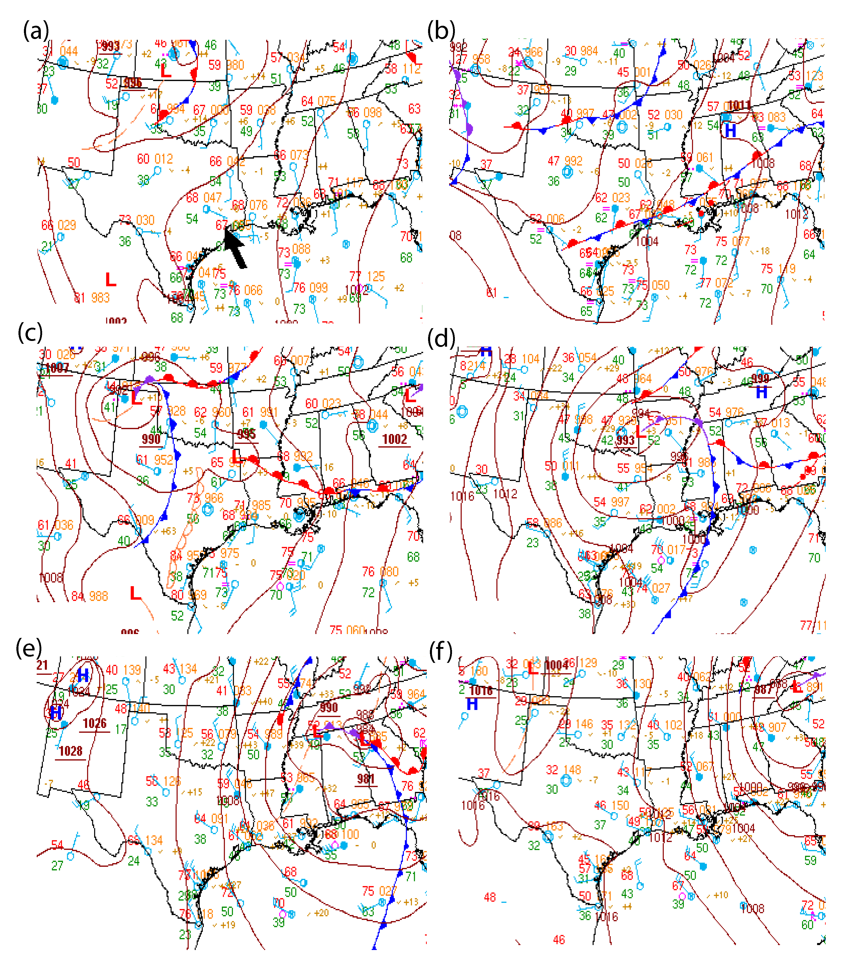
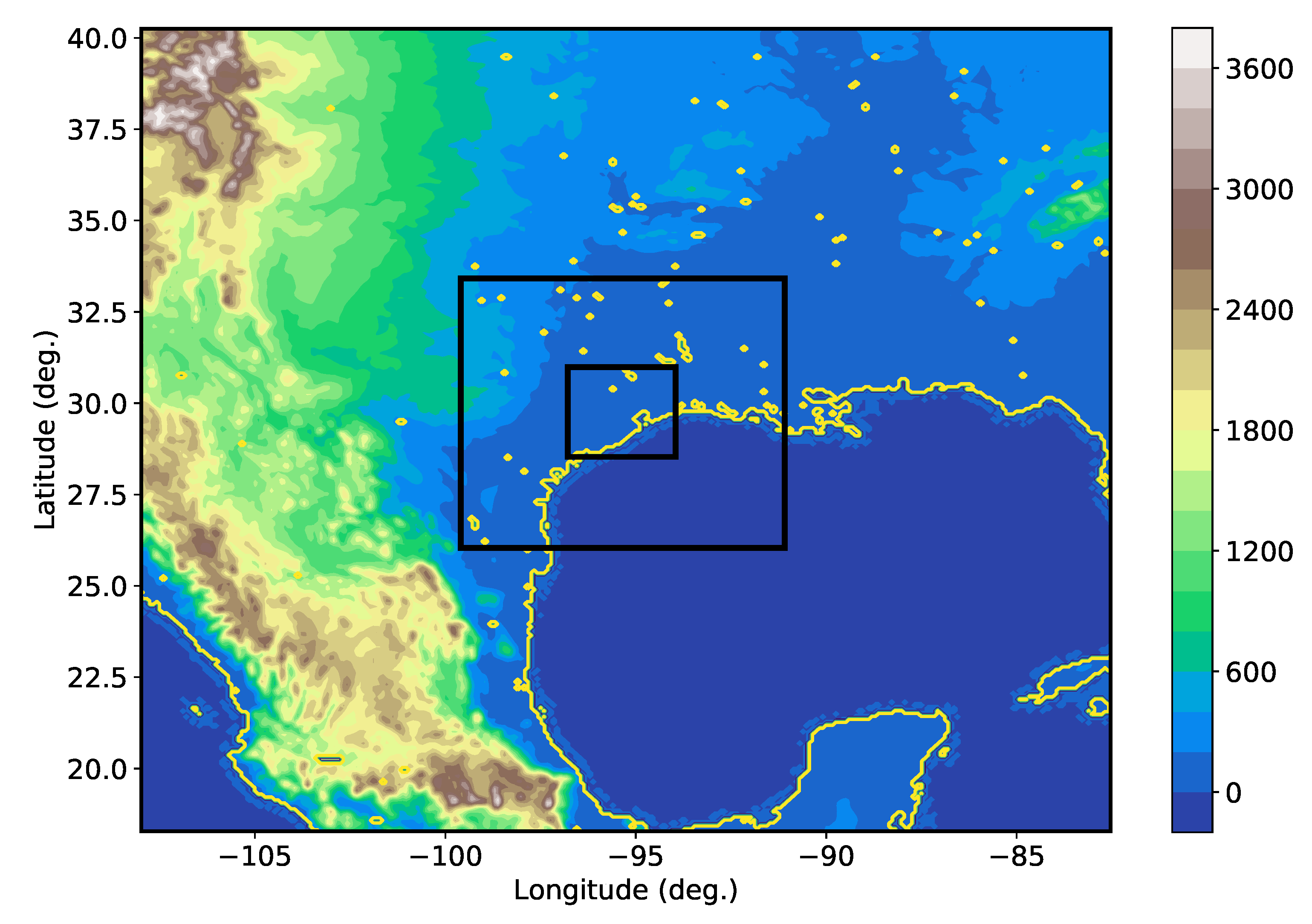
2. Case Study
3. Numerical Simulations and Observational Data
3.1. Description of Numerical Simulations
3.2. Observational Data
4. Results
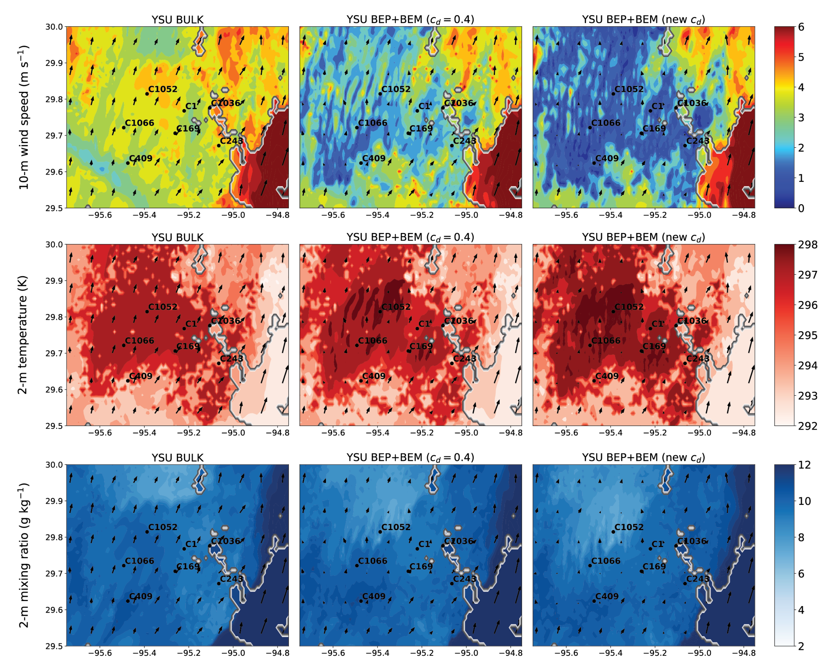
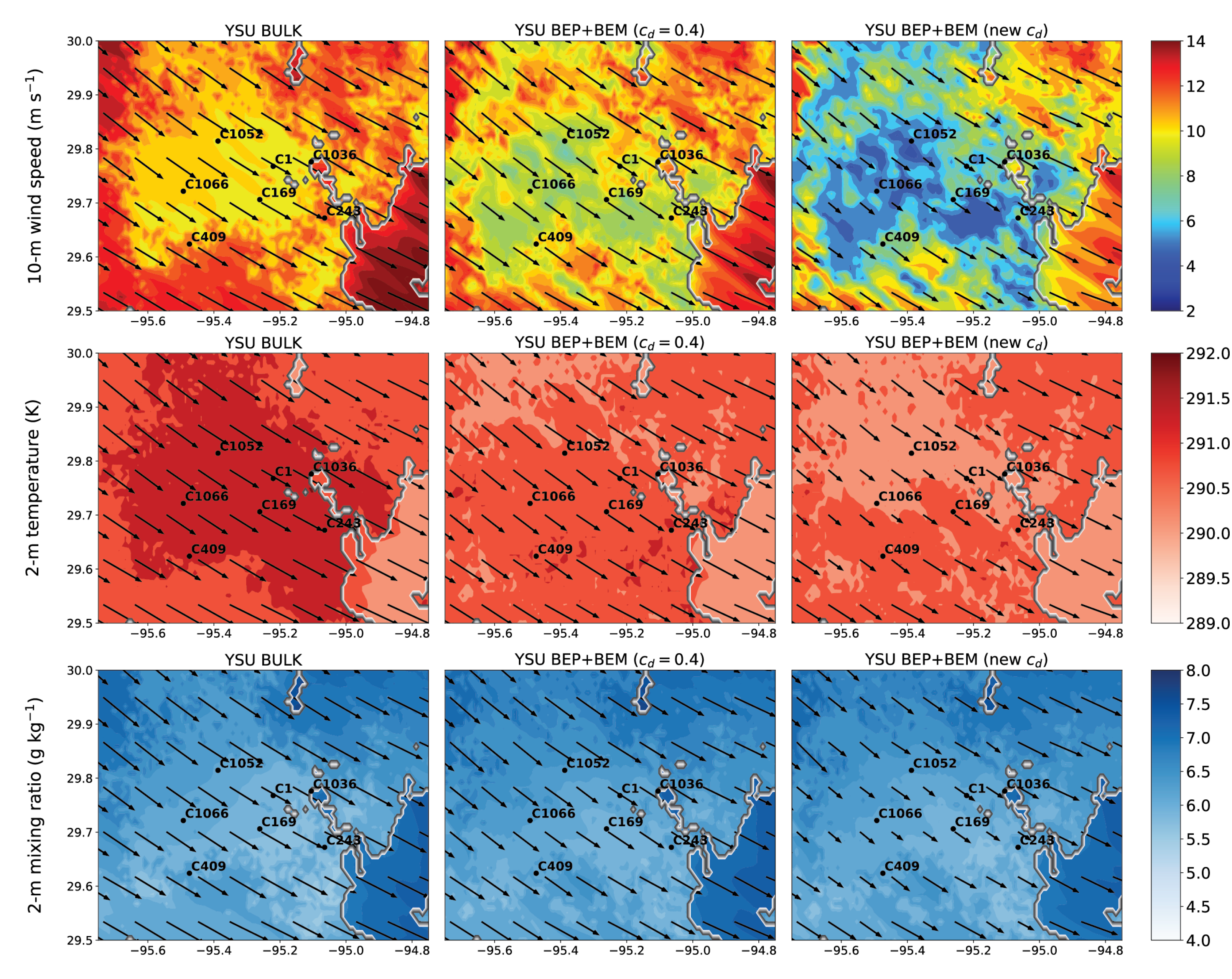
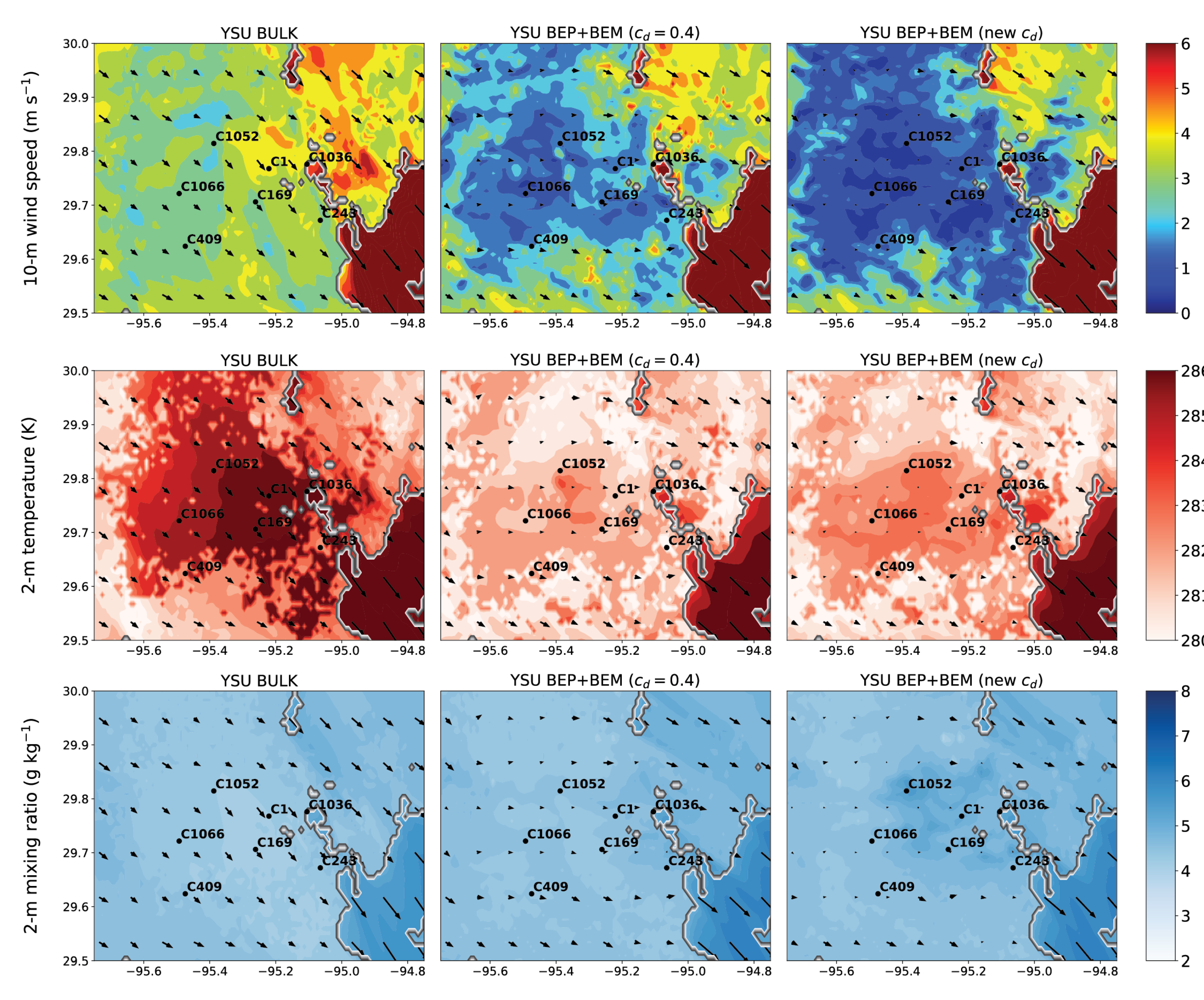
4.1. Near-Surface Forecasts in the Urban Environment
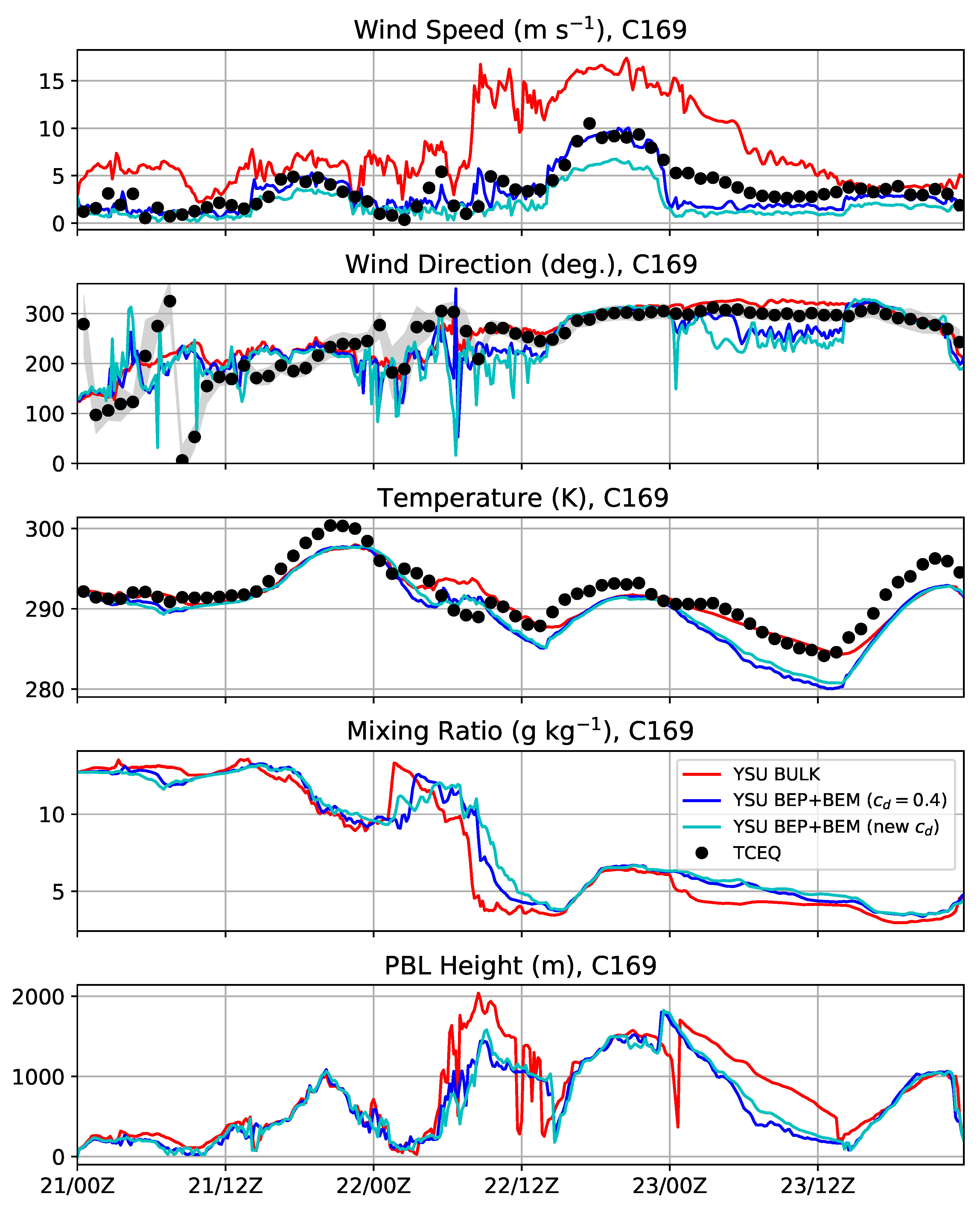
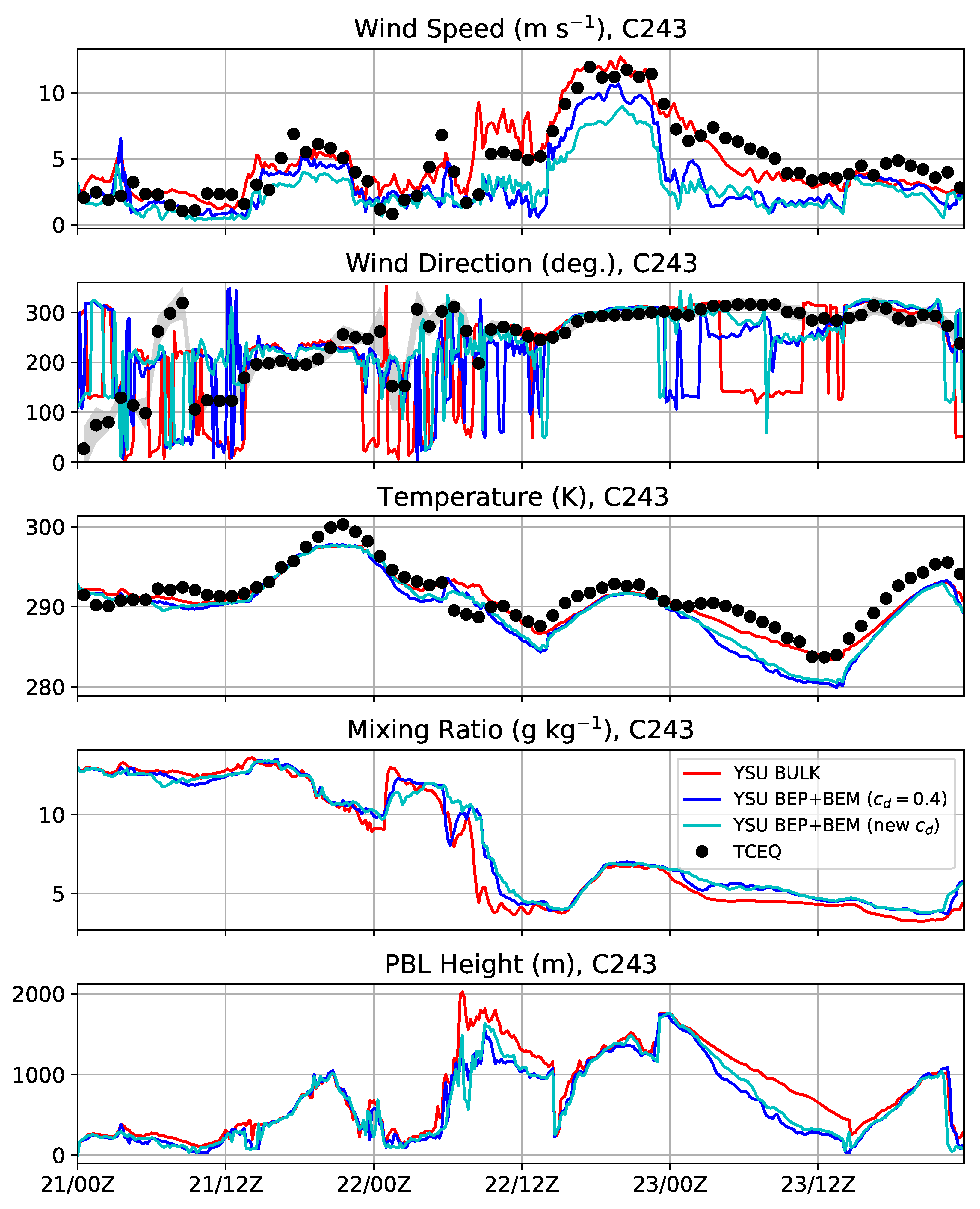
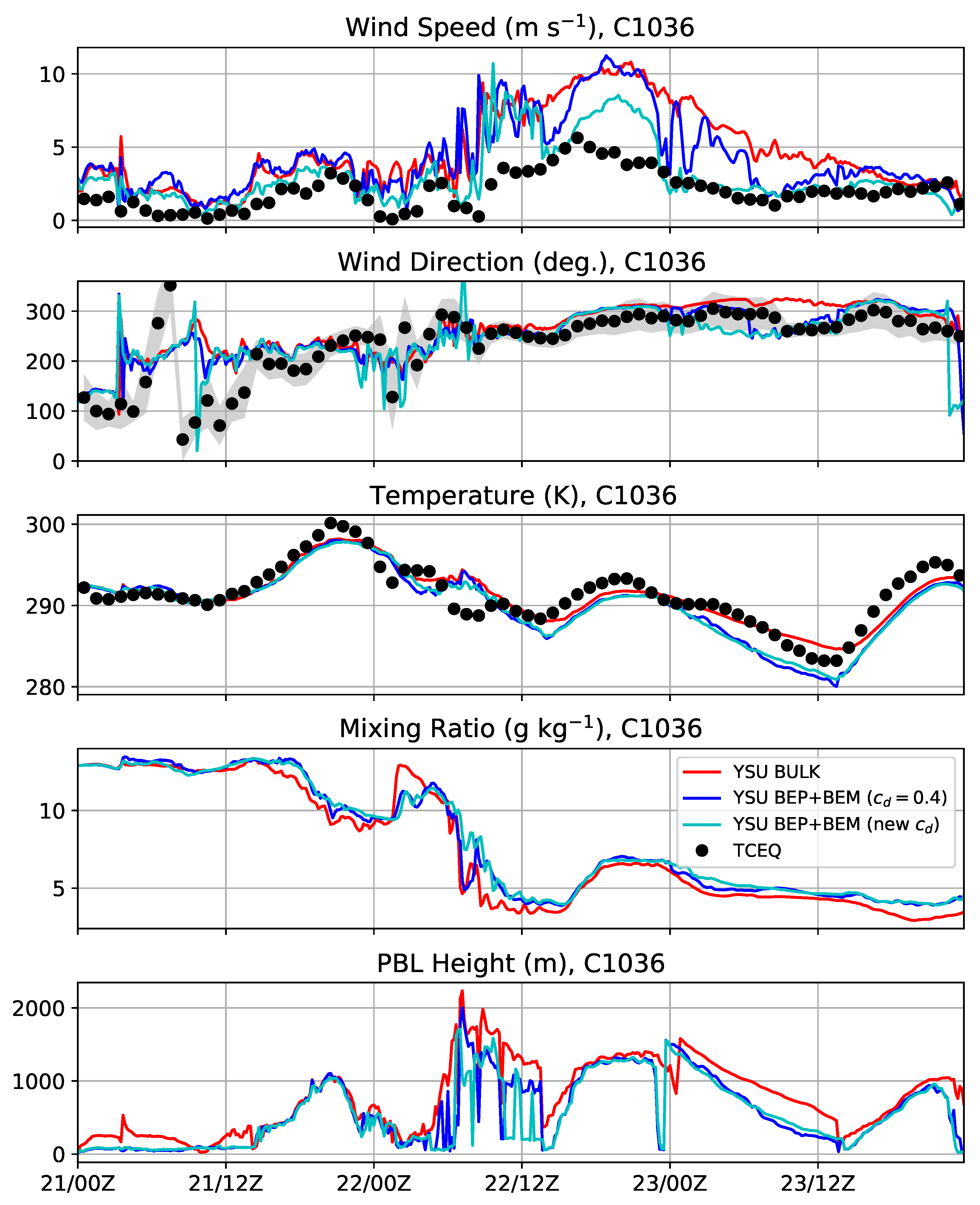
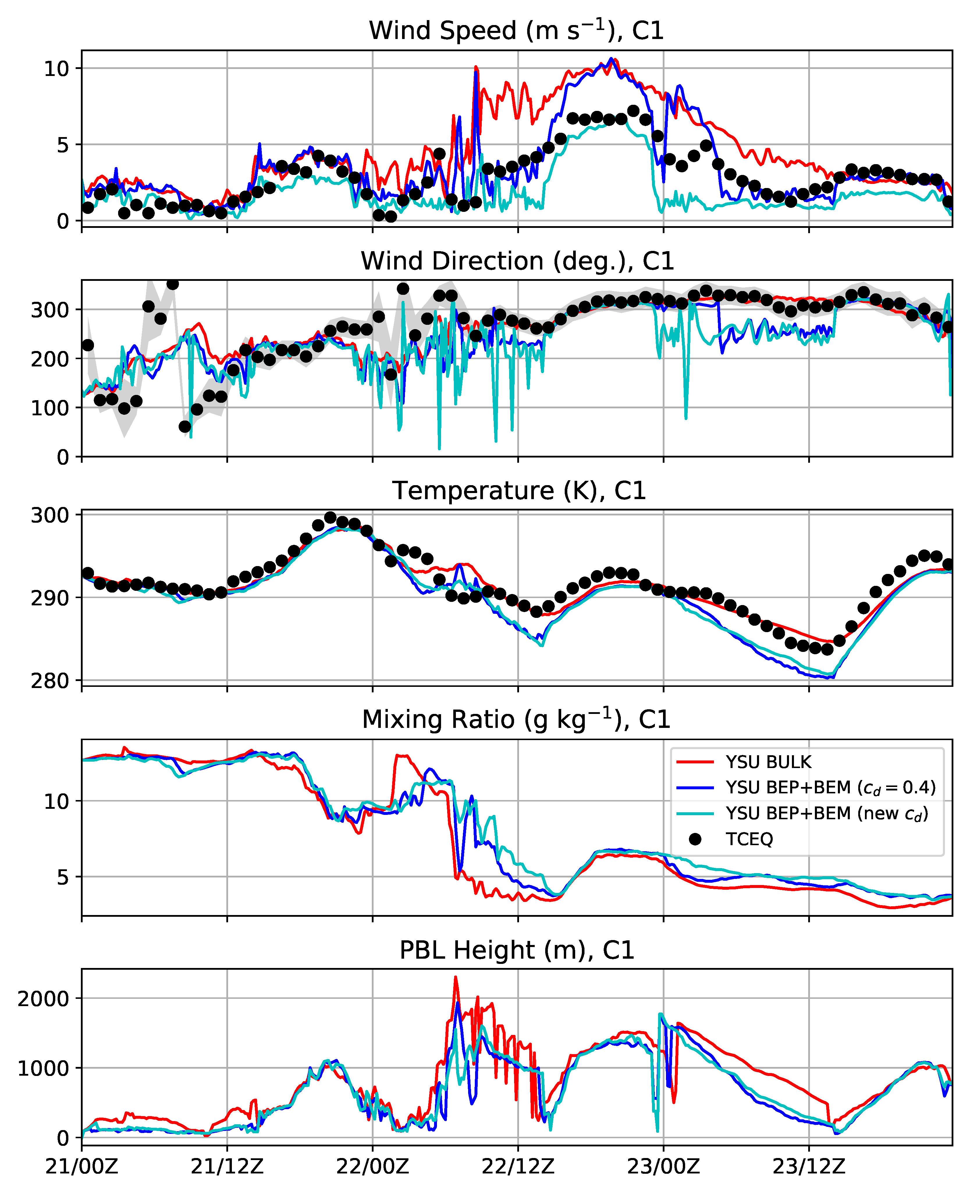
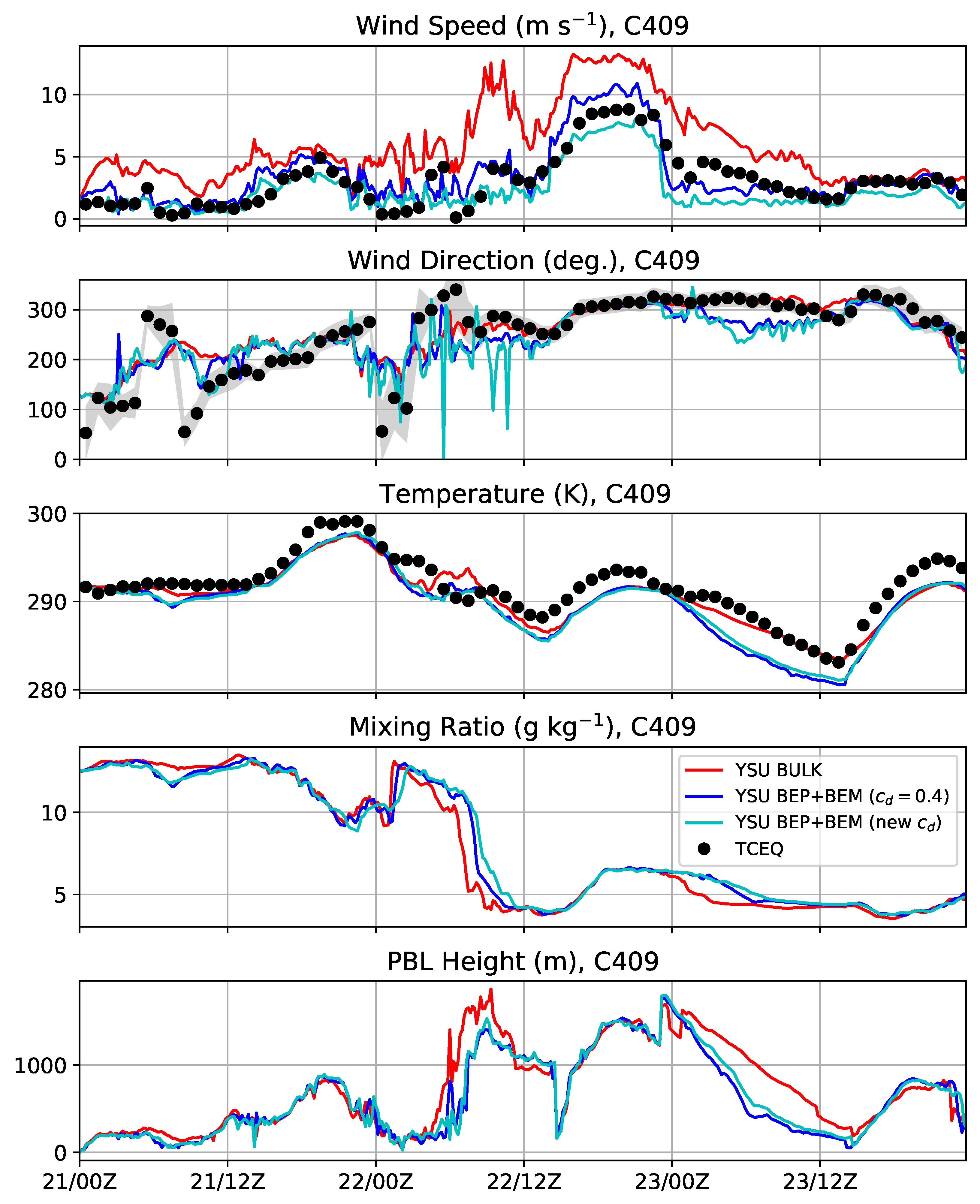
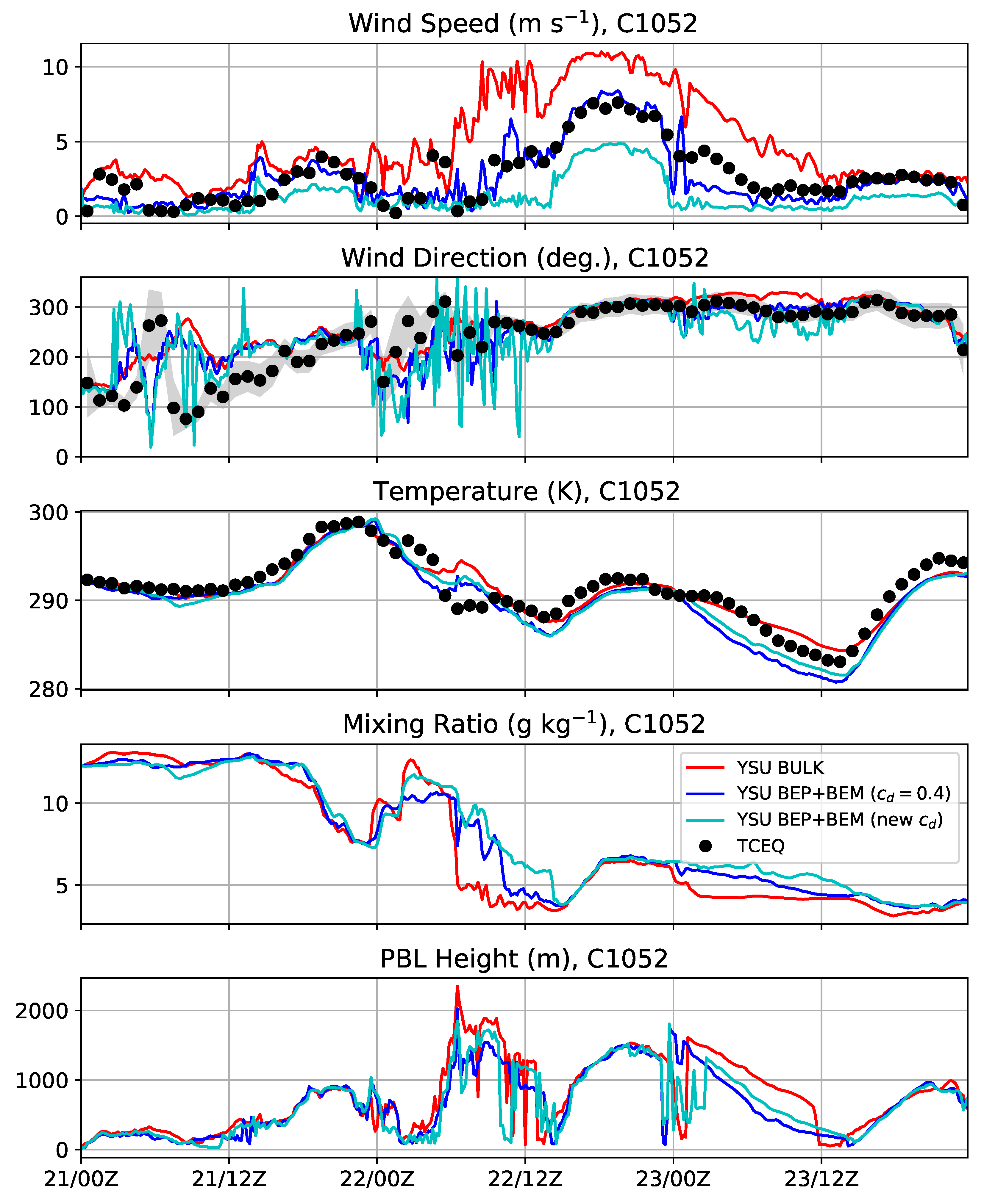
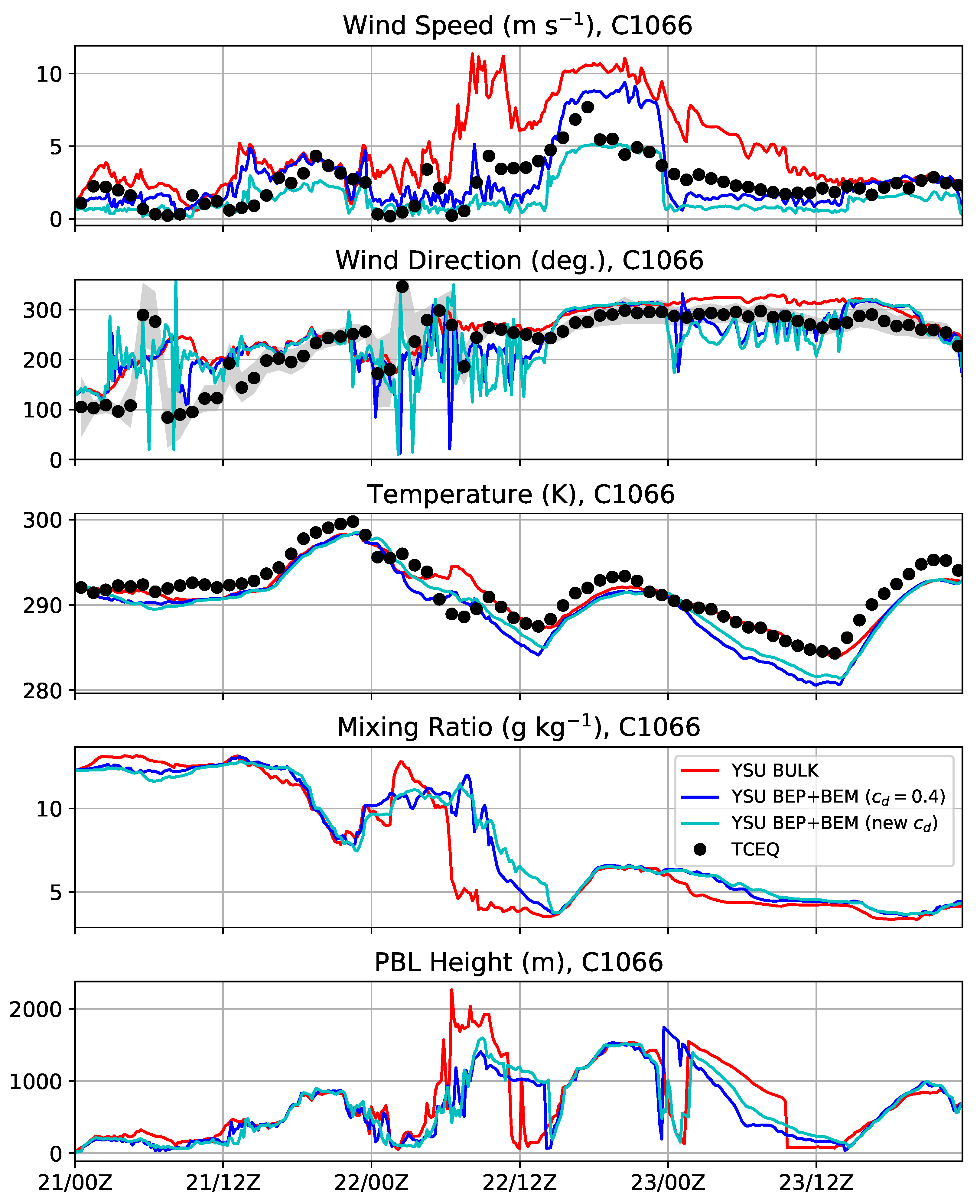
4.2. Time Series
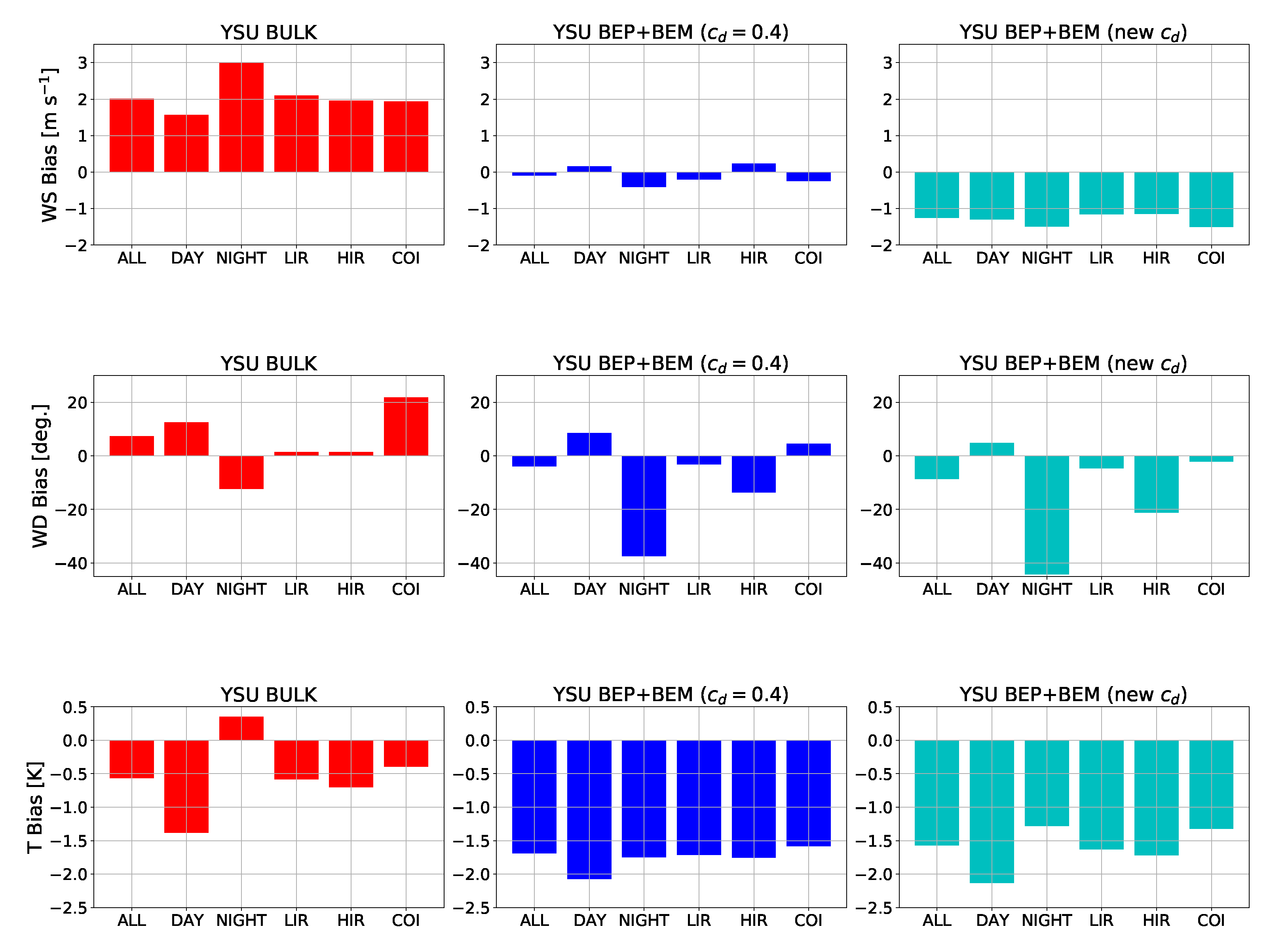
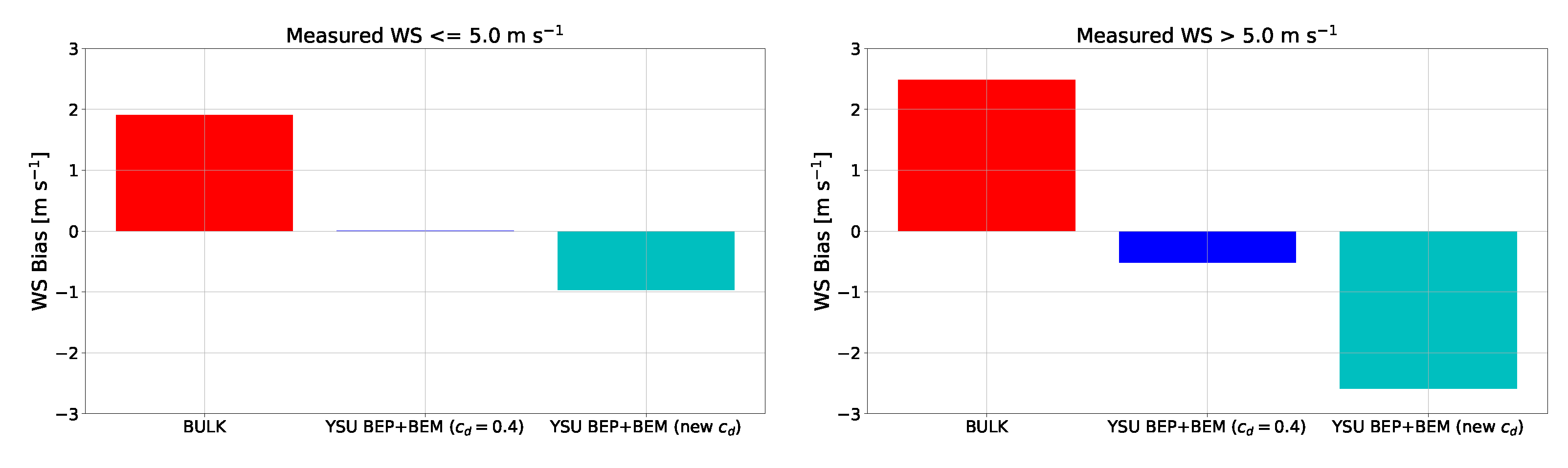
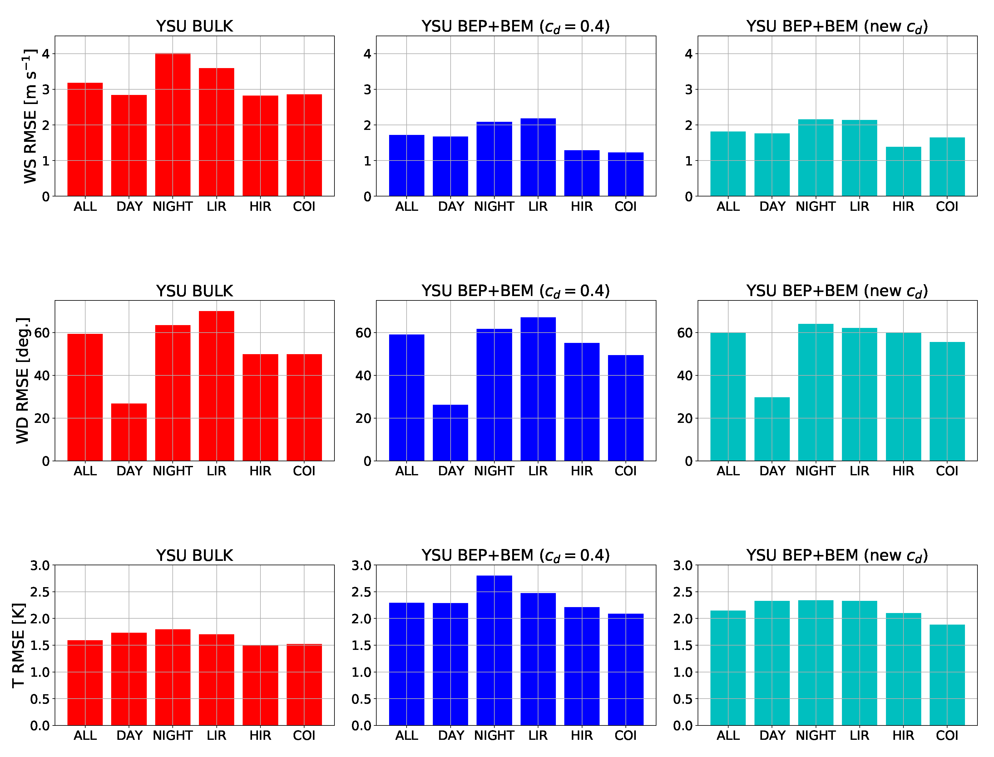
4.3. Performance Measures
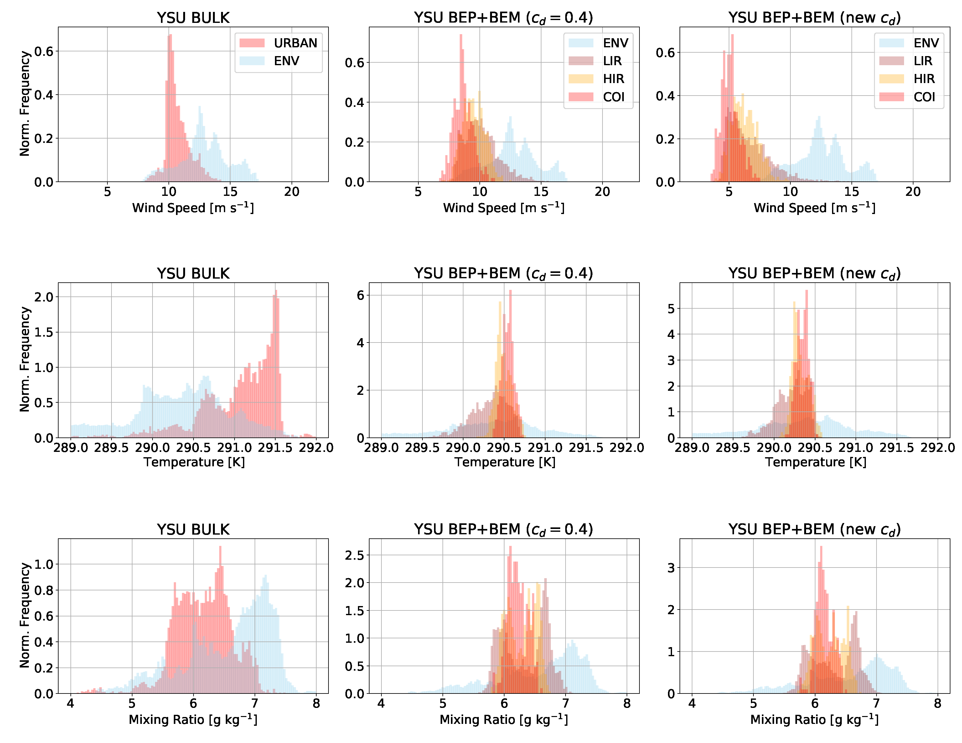
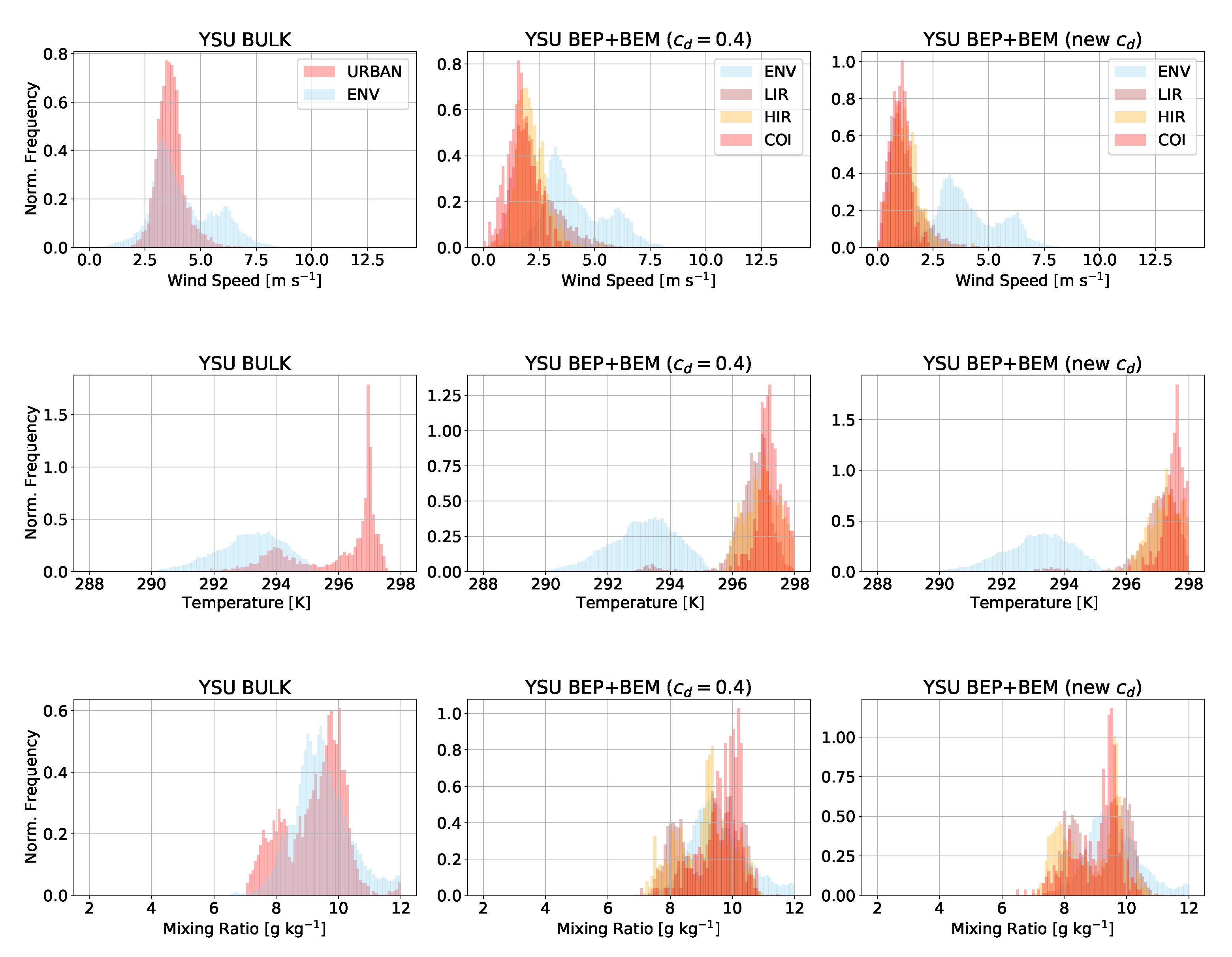
4.4. Variability of Near-Surface Forecasts by Land Use
5. Discussion and Conclusions
Author Contributions
Funding
Institutional Review Board Statement
Informed Consent Statement
Data Availability Statement
Acknowledgments
Conflicts of Interest
Abbreviations
| AGL | above ground level |
| BEP | Building Effect Parameterization |
| BEM | Building Energy Model |
| COI | commercial and industrial |
| GDAS | Global Data Assimilation System |
| HIR | high intensity residential |
| IGBP | International Geosphere-Biosphere Programme |
| LIR | low intensity residential |
| LST | local standard time |
| ME | mean error |
| MODIS | Moderate Resolution Imaging Spectroradiometer |
| MSLP | mean sea level pressure |
| NCAR | National Center for Atmospheric Research |
| NCEP | National Centers for Environmental Prediction |
| NUDAPT | National Urban Data and Access Portal Tool |
| PBL | planetary boundary layer |
| RDA | Research Data Archive |
| RMSE | root mean squared error |
| RRTMG | Rapid Radiative Transfer Model GCMs |
| TCEQ | Texas Commission on Environmental Quality |
| TKE | turbulent kinetic energy |
| UCM | urban canopy model |
| UTC | Coordinated Universal Time |
| WPC | Weather Prediction Center |
| WRF | Weather Research and Forecasting |
| YSU | Yonsei University |
References
- Oke, T.R. The energetic basis of the urban heat island. Q. J. R. Meteorol. Soc. 1982, 108, 1–24. [Google Scholar] [CrossRef]
- Zhang, N.; Wang, Y.; Lin, X. Mesoscale observational analysis of isolated convection associated with the interaction of the sea breeze front and the gust front in the context of the urban heat humid island effect. Atmosphere 2022, 13, 603. [Google Scholar] [CrossRef]
- Rozoff, C.M.; Cotton, W.R.; Adegoke, J.O. Simulation of St. Louis, Missouri, land use impacts on thunderstorms. J. Appl. Meteor. Clim. 2003, 42, 716–738. [Google Scholar] [CrossRef]
- Peterson, T.C.; Owen, T.W. Urban heat island assessment: Metadata are important. J. Clim. 2005, 18, 2637–2646. [Google Scholar] [CrossRef]
- Zhong, S.; Yang, X.-Q. Mechanism of urbanization impact on a summer cold-frontal rainfall process in the greater Beijing metropolitan area. J. Appl. Meteor. Clim. 2015, 54, 1234–1247. [Google Scholar] [CrossRef]
- Eastin, M.D.; Baber, M.; Boucher, A.; Bari, S.D.; Hubler, R.; Stimac-Spalding, B.; Winesett, T. Temporal variability of the Charlotte (sub)urban heat island. J. Appl. Meteor. Clim. 2018, 51, 81–102. [Google Scholar] [CrossRef]
- Liu, J.; Niyogi, D. Meta-analysis of urbanization impact on rainfall modification. Sci. Rep. 2019, 9, 7301. [Google Scholar] [CrossRef]
- Vukovich, F.M. Theoretical analysis of the effect of mean wind and stability on a heat island circulation characeteristic of an urban complex. Mon. Weather Rev. 1971, 99, 919–926. [Google Scholar] [CrossRef]
- Martilli, A.; Clappier, A.; Rotach, M.W. An urban surface exchange parametrization for mesoscale models. Bound.-Layer Meteorol. 2002, 104, 261–304. [Google Scholar] [CrossRef]
- Salamanca, F.; Krpo, A.; Martilli, A.; Clappier, A. A new building energy model coupled with an urban canopy parameterization for urban climate simulations—Part I. Formulation, verification, and sensitivity analysis of the model. Theor. Appl. Climatol. 2011, 99, 331–344. [Google Scholar] [CrossRef]
- Wang, J.; Mao, J.; Zhang, Y.; Cheng, T.; Yu, Q.; Tan, J.; Ma, W. Simulating the effects of urban parameterizations on the passage of a cold front during a pollution episode in megacity Shanghai. Atmosphere 2019, 10, 79. [Google Scholar] [CrossRef]
- Holt, T.; Pullen, J. Urban canopy modeling of the New York City metropolitan area: A comparison and validation of single- and multilayer parameterizations. Mon. Weather Rev. 2007, 135, 1906–1930. [Google Scholar] [CrossRef]
- Martilli, A. Numerical study of urban impact on boundary layer structure: Sensitivity to wind speed, urban morphology, and rural soil moisture. J. Appl. Meteor. Climatol. 2002, 41, 1247–1266. [Google Scholar] [CrossRef]
- Salamanca, F.; Martilli, A.; Tewari, M.; Chen, F. A study of the urban boundary layer using different urban parameterizations and high-resolution urban canopy parameters in WRF. J. Appl. Meteor. Climatol. 2011, 50, 1107–1128. [Google Scholar] [CrossRef]
- Skamarock, W.C.; Klemp, J.B.; Dudhia, J.; Gill, D.O.; Liu, Z.; Berner, J.; Wang, W.; Powers, J.G.; Duda, M.G.; Barker, D.M.; et al. A Description of the Advanced Research WRF Model Version 4; NCAR Technical Note; NCAR/TN-468+STR; National Center for Atmospheric Research: Boulder, CO, USA, 2021; 88p. [Google Scholar] [CrossRef]
- Louis, J.F. A parametric model of vertical eddies fluxes in the atmosphere. Bound.-Layer Meteorol. 1979, 17, 187–202. [Google Scholar] [CrossRef]
- Santiago, J.L.; Martilli, A. A dynamic urban canopy parameterization for mesoscale models based on computational fluid dynamics Reynolds-averaged Navier–Stokes microscale simulations. Bound.-Layer Meteorol. 2010, 137, 417–439. [Google Scholar] [CrossRef]
- Gutierrez, E.; Martilli, A.; Santiago, J.L.; Gonzalez, J.E. A mechanical drag coefficient formulation and urban canopy parameter assimilation technique for complex urban environments. Bound.-Layer Meteorol. 2015, 157, 333–341. [Google Scholar] [CrossRef]
- Hendricks, E.A.; Knievel, J.C.; Wang, Y. Addition of multilayer urban canopy models to a monlocal planetary boundary layer parameterization and evaluation using ideal and real cases. Bound.-Layer Meteorol. 2020, 59, 1369–1392. [Google Scholar] [CrossRef]
- Hong, S.-Y.; Lim, J.-O. The WRF single-moment 6-class microphysics scheme (WSM6). J. Korean Meteorol. Soc. 2006, 42, 129–151. [Google Scholar]
- Hong, S.-Y.; Pan, H.-L. Nonlocal boundary layer vertical diffusion in a Medium Range Forecast model. Mon. Wea. Rev. 1996, 124, 2322–2339. [Google Scholar] [CrossRef]
- Hong, S.-Y.; Noh, Y.; Dudhia, J. A new vertical diffusion package with an explicit treatment of entrainment processes. Mon. Weather Rev. 2006, 134, 2318–2341. [Google Scholar] [CrossRef]
- Zhang, C.; Wang, Y. Projected future changes of tropical cyclone activity over the western north and south Pacific in a 20-km-mesh regional climate model. J. Clim. 2017, 30, 5923–5941. [Google Scholar] [CrossRef]
- Chen, F.; Kusaka, H.; Bornstein, R.; Ching, J.; Grimmond, C.S.B.; Grossman-Clarke, S.; Loridan, T.; Manning, K.W.; Martilli, A.; Miao, S.; et al. The integrated WRF/urban modeling system: Development, evaluation, and applications to the urban environmental problems. Int. J. Climatol. 2011, 31, 273–288. [Google Scholar] [CrossRef]
- Ching, J.; Brown, M.; Burian, S.; Chen, F.; Cionco, R.; Hanna, A.; Hultgren, T.; McPherson, T.; Sailor, D.; Taha, H.; et al. National Urban Database and Access Portal Tool. Bull. Am. Meteorol. Soc. 2009, 90, 1157–1168. [Google Scholar] [CrossRef]
- Mellor, G.L.; Yamada, T. Development of a turbulence closure model for geophysical fluid problems. Rev. Geophys. Space Phys. 1982, 20, 851–875. [Google Scholar] [CrossRef]
- Janjić, Z.I. The step-mountain eta coordinate model: Further developments of the convection, viscous sublayer, and turbulence closure schemes. Mon. Weather Rev. 1994, 122, 927–945. [Google Scholar] [CrossRef]
- Bougeault, P.; Lacarrere, P. Parameterization of orography-induced turbulence in a mesobeta-scale model. Mon. Weather Rev. 1989, 117, 1872–1890. [Google Scholar] [CrossRef]


| Parameter | LIR | HIR | COI |
|---|---|---|---|
| Roof/Wall heat capacity (J m−3 K−1) | |||
| Ground heat capacity (J m−3 K−1) | |||
| Roof/Wall thermal conductivity (J m−1 s−1 K−1) | 0.695 | 0.695 | 0.695 |
| Road thermal conductivity (J m−1 s−1 K−1) | 0.4004 | 0.4004 | 0.4004 |
| Roof/Wall surface albedo | 0.20 | 0.20 | 0.20 |
| Road surface albedo | 0.15 | 0.15 | 0.15 |
| Roof/Wall surface emissivity | 0.90 | 0.90 | 0.90 |
| Road surface emissivity | 0.95 | 0.95 | 0.95 |
| Roof/Road momentum roughness length (m) | 0.01 | 0.01 | 0.01 |
| Wall momentum roughness length (m) | 0.0001 | 0.0001 | 0.0001 |
| A/C coefficient of performance | 3.5 | 3.5 | 3.5 |
| Window coverage area | 0.20 | 0.20 | 0.20 |
| Thermal efficiency of heat exchanger | 0.75 | 0.75 | 0.75 |
| Fraction of buildings installed with A/C systems | 1.0 | 1.0 | 1.0 |
| Fraction of cooled floor area in buildings | 1.0 | 1.0 | 1.0 |
| Target temperature of A/C system (K) | 298 | 298 | 298 |
| Peak occupants per urban floor area | 0.10 | 0.10 | 0.20 |
| Comfort range of indoor temperature (K) | 0.5 | 0.5 | 0.5 |
| Target humidity of A/C systems (kg kg−1) | 0.005 | 0.005 | 0.005 |
| Peak heat generated by equipments (W m−2) | 16 | 20 | 36 |
| ID | Latitude | Longitude | Sampling Height (m) | Urban Class | Urban Fraction |
|---|---|---|---|---|---|
| C1 | 29.767778 | −95.220556 | 9.1 | HIR | 0.736 |
| C169 | 29.706111 | −95.261111 | 11.0 | LIR | 0.350 |
| C243 | 29.672000 | −95.064700 | 6.0 | LIR | 0.354 |
| C409 | 29.623889 | −95.474167 | 18.0 | HIR | 0.549 |
| C1036 | 29.776100 | −95.105100 | 7.9 | LIR | 0.458 |
| C1052 | 29.814530 | −95.387690 | 13.5 | COI | 0.847 |
| C1066 | 29.721600 | −95.492650 | 13.0 | COI | 0.934 |
| Land Use Index | Land Use Description |
|---|---|
| 1 | Evergreen Needleleaf Forest |
| 2 | Evergreen Broadleaf Forest |
| 3 | Deciduous Needleleaf Forest |
| 4 | Deciduous Broadleaf Forest |
| 5 | Mixed Forests |
| 6 | Closed Shrublands |
| 7 | Open Shrublands |
| 8 | Woody Savannas |
| 9 | Savannas |
| 10 | Grasslands |
| 11 | Permanent Wetlands |
| 12 | Croplands |
| 13 | Urban and Built-Up |
| 14 | Cropland/Natural Vegetation Mosaic |
| 15 | Snow and Ice |
| 16 | Barren or Sparsely Vegetated |
| 17 | Water |
| 18 | Wooded Tundra |
| 19 | Mixed Tundra |
| 20 | Barren Tundra |
| 31 | Low Intensity Residential |
| 32 | High Intensity Residential |
| 33 | Industrial or Commercial |
Publisher’s Note: MDPI stays neutral with regard to jurisdictional claims in published maps and institutional affiliations. |
© 2022 by the authors. Licensee MDPI, Basel, Switzerland. This article is an open access article distributed under the terms and conditions of the Creative Commons Attribution (CC BY) license (https://creativecommons.org/licenses/by/4.0/).
Share and Cite
Hendricks, E.A.; Knievel, J.C. Evaluation of Urban Canopy Models against Near-Surface Measurements in Houston during a Strong Frontal Passage. Atmosphere 2022, 13, 1548. https://doi.org/10.3390/atmos13101548
Hendricks EA, Knievel JC. Evaluation of Urban Canopy Models against Near-Surface Measurements in Houston during a Strong Frontal Passage. Atmosphere. 2022; 13(10):1548. https://doi.org/10.3390/atmos13101548
Chicago/Turabian StyleHendricks, Eric A., and Jason C. Knievel. 2022. "Evaluation of Urban Canopy Models against Near-Surface Measurements in Houston during a Strong Frontal Passage" Atmosphere 13, no. 10: 1548. https://doi.org/10.3390/atmos13101548
APA StyleHendricks, E. A., & Knievel, J. C. (2022). Evaluation of Urban Canopy Models against Near-Surface Measurements in Houston during a Strong Frontal Passage. Atmosphere, 13(10), 1548. https://doi.org/10.3390/atmos13101548