Article

Estimating FAO Blaney-Criddle b-Factor Using Soft Computing Models

1
Center of Excellence in Sustainable Disaster Management (CESDM), Walailak University, 222, Thaiburi, Thasala, Nakhon Si Thammarat 80160, Thailand
2
School of Languages and General Education, Walailak University, 222, Thaiburi, Thasala, Nakhon Si Thammarat 80160, Thailand
3
School of Engineering and Technology, Walailak University, 222, Thaiburi, Thasala, Nakhon Si Thammarat 80160, Thailand
4
Civil Engineering Department, College of Engineering, Najran University, King Abdulaziz Road, P.O. Box 1988, Najran 66291, Saudi Arabia
5
Institute of Applied Technology, Thu Dau Mot University, Thu Dau Mot 75000, Binh Duong, Vietnam
*
Authors to whom correspondence should be addressed.
Atmosphere 2022, 13(10), 1536; https://doi.org/10.3390/atmos13101536
Submission received: 31 July 2022 / Revised: 15 September 2022 / Accepted: 15 September 2022 / Published: 20 September 2022

Abstract

:
FAO Blaney-Criddle has been generally an accepted method for estimating reference crop evapotranspiration. In this regard, it is inevitable to estimate the b-factor provided by the Food and Agriculture Organization (FAO) of the United Nations Irrigation and Drainage Paper number 24. In this study, five soft computing methods, namely random forest (RF), M5 model tree (M5), support vector regression with the polynomial function (SVR-poly), support vector regression with radial basis function kernel (SVR-rbf), and random tree (RT), were adapted to estimate the b-factor. And Their performances were also compared. The suitable hyper-parameters for each soft computing method were investigated. Five statistical indices were deployed to evaluate their performance, i.e., the coefficient of determination (r2), the mean absolute relative error (MARE), the maximum absolute relative error (MXARE), the standard deviation of the absolute relative error (DEV), and the number of samples with an error greater than 2% (NE > 2%). Findings reveal that SVR-rbf gave the highest performance among five soft computing models, followed by the M5, RF, SVR-poly, and RT. The M5 also derived a new explicit equation for b estimation. SVR-rbf provided a bit lower efficacy than the radial basis function network but outperformed the regression equations. Models’ Applicability for estimating monthly reference evapotranspiration (ETo) was demonstrated.

1. Introduction

Reference evapotranspiration (ETo) estimation is imperative information to serve water resources planning, management, and operation [1]. The Blaney-Criddle method, as proposed by the Food and Agricultural Organization (FAO) of the United Nations, is a well-known temperature-based reference crop evapotranspiration. This method gives more advantage when having limitations of the measured data than the Penman-Monteith method, which requires many meteorological data [2,3,4]. Many attempts [5,6,7,8,9] have been made to evaluate the efficiency of the FAO Blaney-Criddle method in estimating reference crop evapotranspiration for many regions. The study results by Jhajharia, Ali, DebBarma, Durbude, and Kumar [6] revealed that in humid locations, the Blaney-Criddle method was superior to other temperature-based methods, such as Hargreaves and Thornth–Waite. This is because it offered an approximate solution of the reference crop evapotranspiration closest to the FAO Penman-Monteith. However, the calibration of FAO-Blaney-Criddle parameters by the use of meteorological data in the corresponding region is important as they differ from location to location [10]. In addition, the Blaney-Criddle approach has been updated to suit the environment [11,12].
For many years, soft computing methods have been applied to manage water resource problems and related hydrology issues, especially for predicting evapotranspiration [13,14,15]. Tzimopoulos, Mpallas, and Papaevangelou [14] applied fuzzy logic to establish a temperature-based approach for estimating possible evapotranspiration and compared it to the Blaney-Criddle method. Ramanathan, Saravanan, Adityakrishna, Srinivas, and Selokar [13] found that artificial neural networks (ANN), wavelet neural networks (WNN), and fuzzy logic (FL) yielded better results in estimating ET0 compared to traditional approaches, such as the Penman-Monteith method, the Blaney-Criddle method, and the Hargreaves method. Ferreira et al. [16] indicated that clustering weather stations with analogous hydrological characteristics and lagged time data improved the performance of ANN and support vector machine (SVM) for estimating ET0. Yu et al. [17] pointed out the importance of selecting input patterns by studying its sensitivity analysis and concluded two crucial weather variables for modeling ET0, i.e., maximum and minimum temperature. Shabani et al. [18] indicated that Gaussian Process Regression (GPR) outperformed K-Nearest Neighbors (KNN), Random Forest (RF), and Support Vector Regression (SVR) in predicting pan evaporation. They also emphasized the necessity of suitably choosing weather variables depending on the unique weather station features. Mohammadi and Mehdizadeh [19] revealed hybrid support vector regression with a whale optimization algorithm outperformed a sole support vector regression in modeling reference evapotranspiration, which is a function of air temperatures, relative humidity, solar radiation, sunshine duration, and wind speed. Granata and Di Nunno [20] applied recurrent neural networks to forecast actual evapotranspiration in short term ahead. Their study revealed that in subtropical climatic conditions of South Florida, long short-term memory (LSTM) gave better efficiency than a nonlinear autoregressive network with exogenous inputs (NARX), and there was no significant effect of sensible heat flux and relative humidity on actual evapotranspiration forecasting. On the other hand, in the semi-arid climate of Central Nevada, NARX outperformed LSTM, and there were slight effects due to relative humidity, sensible heat flux, and forecast horizon. Our best literature reviews pointed out the research gap in estimating the b factor of the FAO Blaney-Criddle formula using the soft computing method since only one soft computing method, the Radial Base Function (RBF) network, was researched.
This research article intends to investigate the applicability of soft computing methods in estimating the b factor of the FAO Blaney-Criddle formula, which is advantageous for hydrology and agriculture-related issues. The novelty of this research is the first attempt to use random forest (RF), M5 model tree (M5), support vector regression (SVR) with two kernel functions (i.e., polynomial and radial), and random tree (RT) for estimating the b factor. Their performance was compared with the previous studies. Each model’s weaknesses and advantages were discussed. The rest of this article is organized as follows: the next section explains the method and data used, including FAO Blaney-Criddle b factor, soft computing models, Weka machine learning tool, tuning hyper-parameters, data used, and statistical model performance indices. Section 3 provides the significant finding results of the suitable hyper-parameters for each soft computing method and their comparative performance among five soft computing methods as conducted in the present study and the previous studies. Our main study’s finding is concluded and recommended in the final section.

2. Materials and Methods

2.1. FAO Blaney-Criddle B Factor

The original Blaney-Criddle equation requires information on the average daily percentage of total daily hours and mean daily air temperature for predicting reference crop evapotranspiration. Its formula is expressed as follows, by [21].
E T 0 = a + b p 0.46 T + 8.13
where ET0 is reference crop evapotranspiration (mm/d); a and b are calibrated constants; p is the average daily percentage of total annual daytime hours; and T is the average daily air temperature (°C). The a factor can be derived by:
a = 0.0043 R H m i n n / N 1.41
where RHmin is the lowest daily relative humidity (%); and n/N is the average ratio of actual to possible sunshine hours. The p and N values can be received from tables when specifying latitudes and months [21,22]. They can be obtained using formulas as proposed by [23,24].
For determination of the value of b factor, Doorenbos, Pruitt, and Agl [21] proposed it in tabular form. It depends on the lowest daily relative humidity (RHmin), daytime wind speed (Ud), and the average ratio of actual to possible sunshine hours (n/N) (see detailed information in Table 1). The authors can simply utilize the technique of table interpolation to obtain the b value. However, it needs seven interpolation times for getting that value, leading to lead to considerable error [25]. To defeat such drawback, Frevert et al. [26] first proposed a regression equation (see Equation (3)) and, later, it was improved by Allen and Pruitt [27] (see Equation (4)). Nevertheless, it was still an error in estimating the b value of approximately 10% compared to the tabular values. Ambas and Evanggelos [28] used weighted least squares to estimate b factor of the FAO24 Blaney-Criddle method as shown in Equation (5). It gave close results as compared to the previous studies. Equations (3)–(5) still have an error in estimating the b value as compared to the tabular values. Hence, it requires other techniques to decrease the error.
b = 0.81917 0.0040922 R H m i n + 1.0705 n N + 0.065649 U d 0.0059684 R H m i n n / N   0.0005967 R H m i n U d
b = 0.908 0.00483 R H m i n + 0.7949 n N + 0.0768 ln U d   + 1 2 0.0038 R H m i n n N   0.000433 R H m i n U d + 0.281 l n U d + 1 I n n N + 1 0.00975   l n U d + 1   [ l n R H m i n + 1 2 I n   n / N + 1 ]
b = 0.88165 + 0.857596 n N 0.00454 R H m i n + 0.093803 U d 0.00405 R H m i n n N 0.00087 R H m i n U d

2.2. Soft Computing Models

Soft computing models refer to a data analysis of a complex system in order to discover the relationship between system state variables, i.e., independent and dependent variables, without explicit knowledge of the physical nature of the system [29]. In this section, four data-driven models, e.g., random forest (RF), M5 model tree (M5), support vector regression (SVR), and random tree (RT) are briefly explained, as follows.

2.2.1. Random Forest (RF)

The Random Forest (RF) was first introduced by Breiman [30] and has been a common modification of decision trees, which is one of the collections of techniques for data classification and regression [31]. There are two major phases of model construction. In the first step, RF generates a number of individual trees based on the decision tree process. Each tree is created by randomly selecting different sampled training data sets from the entire training data set (also known as the bagging method or bootstrap aggregation) and sub-attributes (or features) from all attributes in the training data set. Second, the voting method is applied, that is, the model prediction is finally achieved by voting for the classification problem or by using the mean value for the regression problem from the predictive performance of each tree generated. In comparison to the M5, full-grown RF trees are not pruned back. This is one of the key benefits of the regression of RF over the M5. As the number of trees increases, the error of speculation still converges even without pruning the tree, and over-fitting is not a matter of concern in light of the Strong Law of Large Numbers [32]. The RF model was adapted based on regression models in this study.

2.2.2. M5 Model Tree (M5)

The M5 Model Tree (M5) model tree was first implemented by Quinlan [33]. It applies a divide-and-conquer method to the creation of a relationship between independent and dependent variables and can be applied to both qualitative (categorical) and quantitative variables. Building M5 involves three stages. The first stage involves the development of a decision tree by dividing the data set into subsets (or leaves). Second, the overgrown tree is reduced, and linear regression functions substitute the plucked sub-trees to avoid overfitting the structure or a weak generalizer. The merging of certain lower sub-trees into one node is processed as part of the pruning approach. The smoothing procedure is finally employed to reduce the serious discontinuities between the linear models in the leaves of the trimmed trees, especially for models created from a small number of training samples.

2.2.3. Support Vector Regression (SVR)

Support Vector Regression (SVR) was developed by Vapnik [34] and his colleagues. This is the adaptation of the support vector machine (SVM) for regression. The basic idea of SVR learning is to solve the separation hyperplane that can correctly divide the training data set and has the largest geometric interval [35,36]. Using the automated conversion of nominal values to numerical values, SVM may be both numerical and nominal. Normalization or standardization shall be processed for all input data prior to the corresponding step. Unlike Support Vector Machine (SVM) for a classifier, which finds a line that best divides training data into classes, SVR processes the best line that separates the training data set by having a minimal error in the cost function. For this reason, an optimization algorithm is used to consider those data instances in the training dataset that are nearest to the minimum cost line. These instances are then referred to as support vectors, which is the name of this technique. In the event that a line that matches the data cannot be identified, a margin is inserted along the line to loosen the constraint. This margin helps the overall outcome to be better, but it does offer some poor predictions to be tolerated. Adequate determination of the complexity parameter C is important. Giving a low C value gives a broad minimum margin, otherwise, it gives a smaller minimum margin. In several real-world problems, it has been found that the use of a straight line is not sufficient for separating data sets. It is also more fitting to use curves or even polygonal regions. By converting data into higher dimensional areas, the kernel functions have been meant to draw lines and predict.

2.2.4. Random Tree (RT)

RT is a fundamental decision tree algorithm collaborating with Quinlan C4.5 or Classification and Regression Trees (CART). It chooses a random subset of attributes for each split from the available attributes before it is implemented with a subset size determined by the part ratio parameter. This method constructs a decision tree and chooses the feature to maximize the information gained using a portion of the data as training data. It is strong and straightforward to use, producing extremely accurate forecasts [29,30]. For a regression tree, a dataset is divided into sub-spaces, and fitting a constant is proceeded for each sub-space [32]. Consequently, A single-tree model exhibits a low level of prediction accuracy and a propensity to be very unstable. However, it can produce extremely accurate results via bagging RT as a decision tree method. It is highly flexible and has quick learning.

2.3. Weka Machine Learning Tool

WEKA (Waikato Environment for Knowledge Analysis) is a Java-based open-source machine learning platform released under the GPL (GNU). It was subsequently established by the University of Waikato in New Zealand. WEKA can impose pre-processing, classification, clustering, association rules, and selection of attributes for data. It also has a graphical representation visualization tool. WEKA has four main applications: Explorer, Experimenter, Knowledgeflow, and SimpleCLI. We can use the Explorer environment to explore the data. If we want to conduct experiments and conduct statistical tests between learning methods, the authors can use an experimenter. Knowledgeflow essentially supports the same features as an explorer, but it is a drag-and-drop interface that supports progressive learning. The authors can work on the WEKA command-line interface in a simpleCLI environment.

2.4. Tuning Hyper-Parameters

Developing a soft computing model or machine learning model considers two parameters, i.e., model parameters and hyper-parameters. Unlike model parameters obtained during the training process, hyper-parameters are the pre-setting parameters by the user to determine model structure before training the models. The control of a machine learning model’s behavior requires hyperparameter adjustment. Therefore, our predicted model parameters will yield less performance if our hyper-parameters aren’t properly tuned to minimize the loss function. In general, the process for tuning hyper-parameters includes defining a model, defining the range of possible values for all hyper-parameters, defining a method for sampling hyper-parameter values, defining evaluative criteria to judge the model, and defining a cross-validation method. In this experiment, a WEKA experimenter was utilized to do a systematic trial and error, that is, varying one interesting parameter and fixing the remained parameters, and repeating this step until covering all parameters. The Root Relative Squared Error (RRSE) with ten-fold cross-validation, given in WEKA, was used as a criterion for selecting the best parameter value for all 216 data sets.

2.5. Data Used

In this study, 216 data sets taken from the b factor tabular of FAO Blaney-Criddle [21] were utilized, coincident with the study purpose. For evaluating the models’ performance with the previous studies, the training and testing process data sets were the same as those used in Trajkovic, Stankovic, and Todorovic [25]. They randomly selected 186 of 216 data sets for training models and used all 216 data sets for testing models. Table 1 summarizes the statistical analysis of relevant parameters of FAO Blaney-Criddle b for the training and testing processes. In overall statistic values, they were very similar for both training and testing data sets. However, when considering the Kurtosis value, it indicated all parameters (Ud, n/N, RHmin, and b) for both training and testing datasets had platykurtic distributions. Also, the skewness value showed that Ud, n/N, and RHmin for both training and testing datasets were approximately symmetric (“-” sign means skewed left and “+” sign means skewed right), while b for both training and testing datasets were moderately skewed right. The correlation analysis was conducted to individually evaluate the strength of the relationship between each input parameter (Ud, n/N, and RHmin) and an output parameter (b). A low degree correlation was found for Ud (r = 0.27, and 0.26 for training and testing stages, respectively), and a high degree correlation was obtained for the rest parameters. The n/N gave the correlation coefficient (r) of 0.57 and 0.58 for the training and testing stages, respectively. Additionally, RHmin provided a strong negative relationship by giving the correlation coefficient (r) of −0.74 for both the training and testing stages, respectively.
Table 1. Statistical evaluation of FAO Blaney-Criddle b parameters for training and testing data sets.
Statistical ValuesTrainingTesting
Udn/NRHminbUdn/NRHminb
Maximum10.001.00100.002.6310.001.00100.002.63
Minimum0.000.000.000.380.000.000.000.38
Average5.010.5149.681.195.010.5049.721.18
Standard Deviation3.420.3434.060.473.420.3434.070.46
Kurtosis−1.27−1.28−1.26−0.09−1.27−1.27−1.260.10
Skewness−0.01−0.050.010.62−0.010.010.010.67
Correlation Coefficient (r)0.270.57−0.741.000.260.58−0.741.00
Number of data186216

2.6. Statistical Model Performance Indices

Five statistical indices were deployed to evaluate model performance, i.e., the coefficient of determination (r2) (Equation (6)), the mean absolute relative error (MARE) (Equation (7)), the maximum absolute relative error (MXARE) (Equation (8)), the standard deviation of the absolute relative error (DEV) (Equation (9)), and the number of samples with an error greater than 2% (NE > 2%). All of these statistical indices were used by Trajkovic, Stankovic, and Todorovic [25] on this particular issue. The r2 calculates the level of linearity of two variables and its maximum is 1.00. MARE and MXARE determine the difference between the real and the expected b factor and should be as small as possible. The perfect model should have an NE of zero. Finally, a Taylor diagram was proposed to comparatively elaborate and evaluate the efficacy of the developed models. This diagram can simultaneously show three statistic parameters, i.e., correlation, root mean square error, and standard deviation. The equations of statistical indices are given below, where b a i is the actual b-factor, is the estimated b-factor, and n is the number of samples in a data set.
r 2 = i = 1 n b a i b ¯ a i b e i b ¯ e i i = 1 n ( b a i b ¯ a i ) 2 · i = 1 n ( b e i b ¯ e i ) 2 2
M A R E = 1 n i = 1 n b a i b e i b a i
M X A R E = m a x b a i b e i b a i   for   i = 1 , , n
D E V = i = 1 n b a i     b e i b a i M A R E 2 n 1

3. Results and Discussion

3.1. Results of Tuning Hyper-Parameters

Table 2 shows the results of tuning hyper-parameters. Their explanation for each soft computing model is as follows.

3.1.1. Random Forest (RF)

In the process of tuning hyper-parameters for RF, some default parameters were selected as default in WEKA software, i.e., (1) infinite maximum tree depth, and (2) int(log 2(#predictors) + 1) function used to set the number of randomly selected attributes. However, three parameters, namely: (1) numIteration, which is the number of trees in the random forest; (2) batchSize, which is the optimum number of instances to be processed when predicting batch; and (3) numExecutionSlots, which is the number of threads available for execution to be used to create the collection, were investigated in our experiment. Findings revealed that numIteration of 300, batchSize of 100 (default value), and numExecutionSlots of 1 (default value) were the suitable hyper-parameters for RF with the testing data set. All cases gave an RRSE value of 12.14. The numIteration was a sensitive parameter, while batchSize and numExecutionSlots were not sensitive.

3.1.2. M5 Model Tree (M5)

The authors experimented tuning hyper-parameters of the M5 model tree using the default parameters in WEKA software of unpruned to be false, and use Unsmoothed to be false. The four parameters, i.e., batchSize, minNumInstances, numDecimalPLaces, and buildRegressionTree were investigated. If the batch prediction is utilized, the bathcSize option specifies the recommended number of instances to process. More or fewer instances are conceivable, but this allows implementations to select the batch size they want. The minimal number of instances to allow at a leaf node is specified by minNumInstances. The number of decimal places to utilize for the model’s output is numDecimalPLaces. It can be decided whether to construct a regression tree/rule instead of a model tree/rule using the buildRegressionTree method.
Findings revealed that batchSize of 100 (default value), minNumInstances of 4 (default value), and numDecimalPLaces of 4 (default value), were the suitable hyper-parameters for M5 with the testing data set. All best cases gave an RRSE value of 11.46. By using batchSize of 100, minNumInstances of 4, and numDecimalPLaces of 4, the authors investigated the effect of selecting or not selecting a regression tree/rule. There was no need to generate a regression tree/rule due to giving an RRSE value of 11.46 compared to creating a regression tree/rule, which gave an RRSE value of 56.26. The minNumInstances and buildRegressionTree were sensitive parameters, while batchSize and numDecimalPLaces were not sensitive.

3.1.3. Support Vector Regression (SVR)

For SVR, two kernel functions, namely the polynomial kernel with variable exponent value and the radial basis function kernel with varying gamma value, were investigated. Also, the complexity parameter (C) was varied between 0.0 and 1.0 to determine the optimum value. The gamma parameter represents the influence of a single training reach, with low values indicating ‘far’ and large values indicating ‘close.’ The inverse of the impact radius of the samples chosen by the model as support vectors are gamma parameters. The modified sequential minimal optimization (SMO) as an iterative algorithm was used to solve the regression problem for SVR [34]. The authors found the optimal hyper-parameters for SVR with polynomial kernel function were the complexity parameter (C) of 0.8 and the exponent (n) of 1.0. By fixing the complexity parameter (C) value of 0.8 and varying the exponent (n) value from 1.0 to 4.0, it was sensitive to the exponent value for SVR with a polynomial kernel function. The best case gave an RRSE value of 24.21.
Furthermore, the optimal hyper-parameters for the radial basis function kernel were the complexity parameter (C) of 1.0 and the gamma parameter (γ) of 1.0. By fixing the complexity parameter (C) value of 1.0 and varying the gamma parameter (γ) value from 1.0 to 4.0, it was sensitive to the gamma parameter (γ) value for the radial basis function kernel. Additionally, the gamma parameter (γ) value of 1.0 gave the least RRSE. For both cases, the suitable C parameters were equal to or more than 0.8. It indicated that these data sets required a smaller minimum margin to separate the data. From those suitable exponents of the polynomial kernel function and gamma parameter of the radial basis function kernel were equal to 1.0, it also manifested that these data sets are not conglomerate data sets and do not require projecting the data into a higher-dimensional space for data separation. The best case gave an RRSE value of 2.37.

3.1.4. Random Tree (RT)

RT was conducted to determine the suitable hyper-parameters and some default parameters were selected as suggested by WEKA software, i.e., (1) unlimited maximum depth of the tree and (2) int(log 2(#predictors) + 1) function used to set the number of randomly selected attributes. However, five parameters, namely batchSize, numDecimalPlaces, minNum, numFolds, and minVarianceProp, were investigated. The batchSize refers to the preferred number of instances to be processed when batch predictions are made. The numberDecimalPlaces is the number of decimal places to be utilized in model output. The minNum means the minimum total weight of the instances in a leaf. The numFolds is configured to determine the quantity of data used. For backfitting, one fold is utilized, and the other is applied for building the tree. The minVarianceProp represents the smallest variance of all data present at a node in regression trees to be divided.
Findings revealed that batchSize of 100 (default value), numDecimalPlaces of 2 (default value), minNum of 1 (default value), numFolds of 0 (default value), and minVarianceProp of 0.001 (default value), were the suitable hyper-parameters for RT with testing data set. All best cases gave an RRSE value of 24.23. The minNum, numFolds, and minVarianceProp were sensitive parameters, while batchSize and numDecimalPLaces were not sensitive.

3.2. Model’s Performance Comparison

After getting the most suitable hyper-parameters for each soft computing model, the authors proceeded to assess their performance in estimating the FAO Blaney-Criddle b factor. As explained earlier, to compare the model’s performance, five statistical indices were used, i.e., the coefficient of determination (r2), the mean absolute relative error (MARE), the maximum absolute relative error (MXARE), the standard deviation of the absolute relative error (DEV), and the number of samples with an error greater than 2% (NE > 2%). This evaluation was only conducted for the testing stage following the study by Trajkovic, Stankovic, and Todorovic [25].
Table 3 shows the comparative results of statistical indices getting from the present and previous studies’ testing stages. By ranking the model with each statistical index and counting the frequency for five soft computing models, it was found that SVR-rbf outperformed the other methods, followed by RF, RT, M5, and SVR-poly. This is because SVR-rbf has the lowest values of MARE (%), MXARE (%), NE > 2%, and DEV (%) and the highest value of r2. By doing the same thing, SVR-rbf, RF, and RT gave better results than the regression-based approach proposed by Frevert, Hill, and Braaten [26], Allen and Pruitt [27], and Ambas and Evanggelos [28], while M5 and SVR-poly gave the lower performance. However, SVR-rbf’s performance as compared to the RBF network was comparable due to providing a bit lower performance.
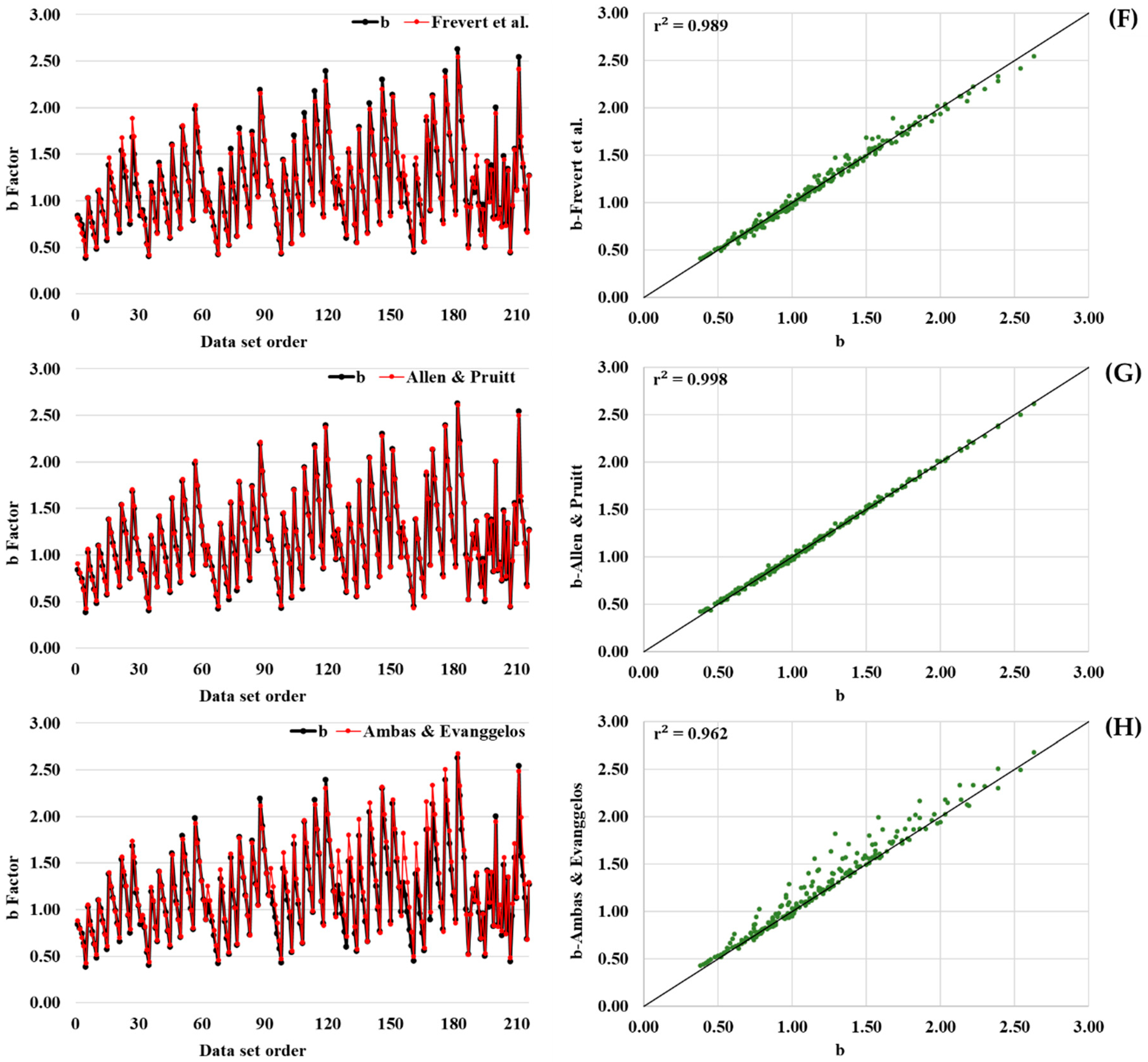
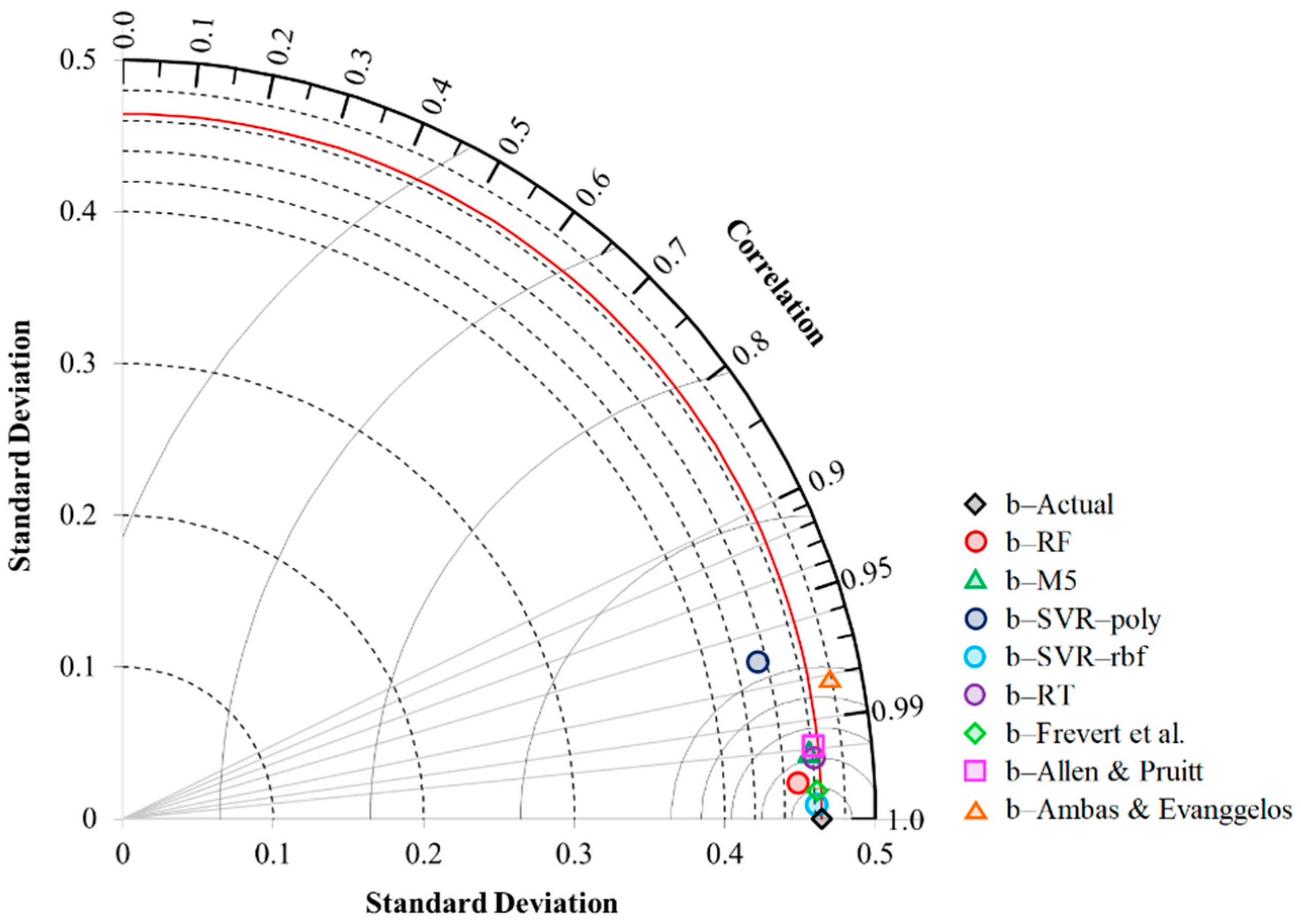
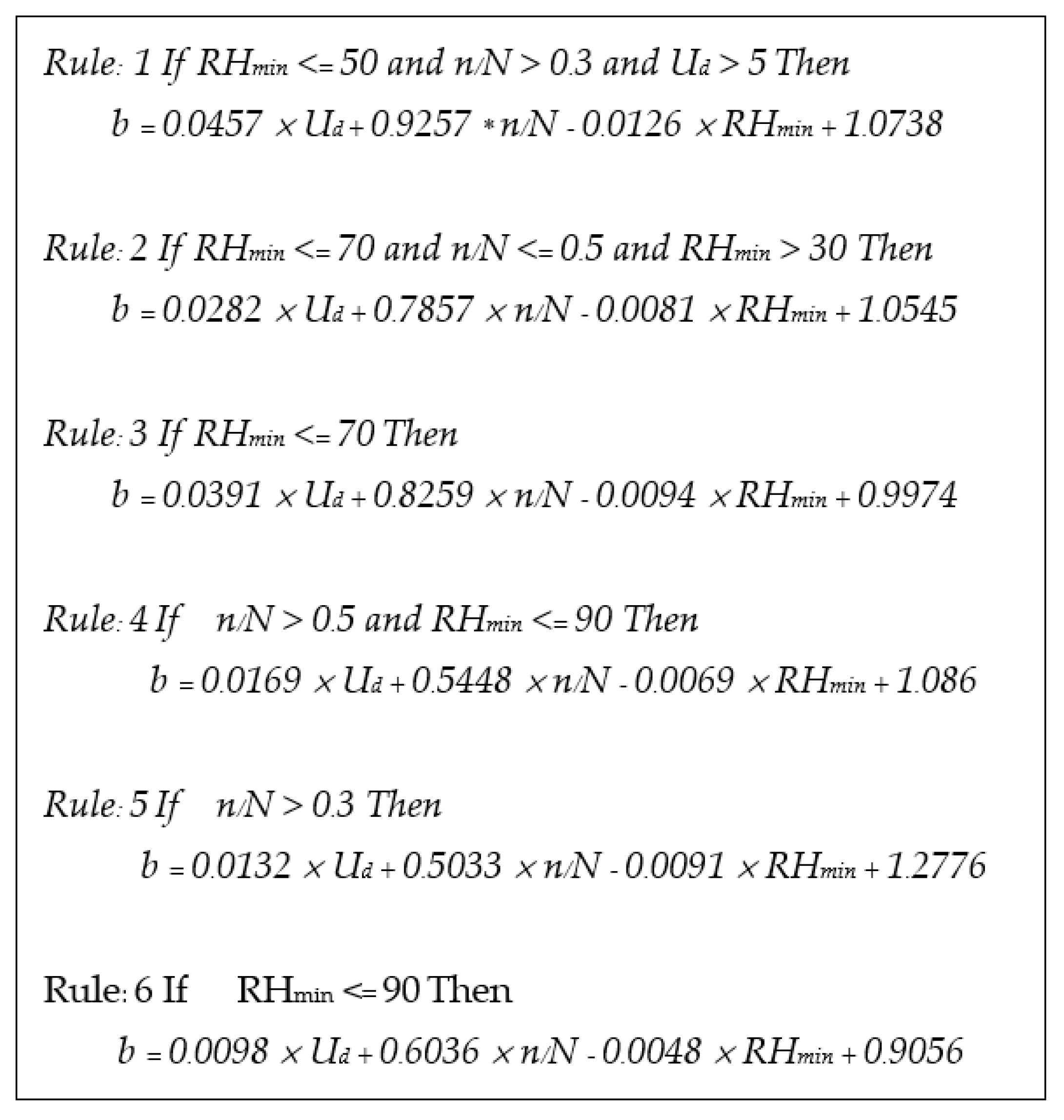
Figure 1 shows the performance of eight models in the testing stage. The left-hand side shows plotting the actual b-factor and estimated b-factor (y-axis) with the data set order (x-axis), and a scatter plot is displayed on the right-hand side. The data set order was received from the b factor tabular of FAO Blaney-Criddle [21] with 216 data sets. The authors could not plot the graph herein for the RBF network due to having no raw predicted data shown in the literature. Figure 2 presents a Taylor diagram to compare the performance of eight models, except for the RBF network, due to the same reason mentioned. Estimating b factor by Frevert, Hill, and Braaten [26], Allen and Pruitt [27], and Ambas and Evanggelos [28] were calculated by Equations (3)–(5), respectively. A Taylor diagram pointed out that SVR-rbf provided the results closest to FAO Blaney-Criddle b parameters obtained from the table as proposed by Doorenbos, Pruitt, and Agl [21], followed by Frevert, Hill, and Braaten [26], RF, RT, M5, Allen and Pruitt [27], Ambas and Evanggelos [28], and SVR-poly. Using the equation proposed by Ambas and Evanggelos [28] and SVR-poly, it gave overestimation and underestimation for the b-factor, respectively, since they have more and less standard deviation (see Figure 2). Consequently, it indicates that these two models gave more uncertainty in estimating the b-factor than other models. Figure 3 shows a set of linear equations obtained from M5. It includes six rule sets.

3.3. Models’ Applicability for Estimating Monthly Reference evapotranspiration (ETo)

The monthly climatological variables at Nis, Yugoslavia, given by Trajkovic, Stankovic, and Todorovic [25], were used to demonstrate the model’s applicability, as shown in Table 4. Reference evapotranspiration (ETo) in January and December is equal to zero. That is why any climatological variables of January and December do not appear in Table 4Table 5 shows the results of applying the developed soft computing models and compares their performance to a table interpolation method [25] and the regression-based models for estimating the b-factor. Table 6 shows the difference between the b-factor obtained from various methods and a table interpolation method. The positive value means overestimation, and the negative value represents underestimation. The b-factor based on the regression-based models was mainly underestimated by 1.12–6.00% compared to those values obtained by the table interpolation method [25], except for estimating the b-factor in June using the equation developed by Frevert et al. [26]. It gave an overestimation of 1.11%. However, most of the soft computing models overestimated by 0.57–3.92% in the estimation of the b-factor. Some of them, for example, M5 provided underestimated by 0.3% in March, 1.57% in April, 3.02% in October, and 2.21% in November.
Table 7 presents the estimated monthly reference evapotranspiration (ETo). Using a table interpolation method as a baseline, it is also pointed out that the soft computing models outperformed the regression-based models in ETo estimation due to giving a lower percentage of yearly difference. All three regression-based models gave underestimation by 3.2–5.1% in estimating ETo, while all six soft computing models provided some overestimation by 0.4–0.9%. Based on the data used in this study, the RBF network and RT models gave the highest performance in estimating ETo due to having the lowest percentage of yearly difference.

4. Conclusions

Accuracy of reference evapotranspiration (ETo) estimation is of importance for agricultural water management. In this study, five soft computing models, namely RF, M5, SVR-poly, SVR-rbf, and RT, were evaluated and compared their performance for estimating FAO Blaney-Criddle b-factor among themselves and the previous studies conducted by the RBF network and three regression equations (Richard G Allen et al., 1991; Frevert et al., 1983; Ambas & Evanggelos (2010). In addition, tuning hyper-parameters for each soft computing model were experimented with to receive its suitable architecture before applying them. The main findings results revealed the following.
(1)
Among five soft computing models, it was found that SVR-rbf gave the highest performance in reference evapotranspiration (ETo) estimation, followed by M5, RF, SVR-poly, and RT, respectively.
(2)
The new explicit equations for FAO Blaney-Criddle b-factor estimation were proposed herein using the M5 model. It is a rule set, including six linear equations.
(3)
Compared to the RBF network [25], SVR-rbf provided a bit lower performance but outperformed three previous regression equations.
(4)
The soft computing models outperformed the regression-based models in the b-factor estimation since they gave the lower values of MARE (%), MXARE (%), NE > 2%, and DEV (%) and the higher value of r2.
(5)
Models’ Applicability for estimating monthly reference evapotranspiration (ETo) revealed that the soft computing models outperformed the regression-based models in ETo estimation owing to the lower percentage of yearly difference. All three regression-based models underestimated ETo, while all six soft computing models slightly overestimated it.
(6)
This work’s usefulness is to support a more accurate and convenient evaluation of reference crop evapotranspiration with a temperature-based approach. It leads to agricultural water demand estimation accuracy as necessary data for water resources planning and management.

Author Contributions

Conceptualization, S.T. and P.D.; methodology, S.T. and P.D.; software P.D., S.P., N.S. and I.E.; formal analysis, S.T., S.P., N.S. and I.E.; writing—original draft preparation, S.T., N.T.T.L. and P.D.; writing—review and editing, P.D., N.T.T.L. and Q.B.P.; project administration, P.D. and Q.B.P.; funding acquisition, N.T.T.L. All authors have read and agreed to the published version of the manuscript.

Funding

The authors are thankful to the Deanship of Scientific Research at Najran University for funding this work under the Research Collaboration Funding program grant code (NU/RC/SERC/11/3).

Institutional Review Board Statement

Not applicable.

Informed Consent Statement

Not applicable.

Data Availability Statement

Data can be requested by contacting the corresponding author, upon reasonable request.

Acknowledgments

The authors are thankful to the Deanship of Scientific Research at Najran University for funding this work under the Research Collaboration Funding program grant code (NU/RC/SERC/11/3).

Conflicts of Interest

The author declares that there is no conflict of interests regarding the publication of this manuscript. In addition, the ethical issues, including plagiarism, informed consent, misconduct, data fabrication and/or falsification, double publication and/or submission, and redundancies have been completely observed by the authors.

References

  1. Xiong, Y.; Luo, Y.; Wang, Y.; Seydou, T.; Xu, J.; Jiao, X.; Fipps, G. Forecasting daily reference evapotranspiration using the Blaney-Criddle model and temperature forecasts. Arch. Agron. Soil Sci. 2015, 62, 790–805. [Google Scholar] [CrossRef]
  2. Tabari, H.; Grismer, M.E.; Trajkovic, S. Comparative analysis of 31 reference evapotranspiration methods under humid conditions. Irrig. Sci. 2013, 31, 107–117. [Google Scholar] [CrossRef]
  3. Mobilia, M.; Longobardi, A. Prediction of potential and actual evapotranspiration fluxes using six meteorological data-based approaches for a range of climate and land cover types. ISPRS Int. J. Geo Inf. 2021, 10, 192. [Google Scholar] [CrossRef]
  4. Hafeez, M.; Chatha, Z.A.; Khan, A.A.; Bakhsh, A.; Basit, A.; Tahira, F. Estimating reference evapotranspiration by Hargreaves and Blaney-Criddle methods in humid subtropical conditions. Curr. Res. Agric. Sci. 2020, 7, 15–22. [Google Scholar] [CrossRef]
  5. Fooladmand, H. Evaluation of Blaney-Criddle equation for estimating evapotranspiration in south of Iran. Afr. J. Agric. Res. 2011, 6, 3103–3109. [Google Scholar]
  6. Jhajharia, D.; Ali, M.; Barma, D.; Durbude, D.G.; Kumar, R. Assessing Reference Evapotranspiration by Temperature-based Methods for Humid Regions of Assam. J. Indian Water Resour. Soc. 2009, 29, 1–8. [Google Scholar]
  7. Mehdi, H.M.; Morteza, H. Calibration of Blaney-Criddle equation for estimating reference evapotranspiration in semiarid and arid regions. Disaster Adv. 2014, 7, 12–24. [Google Scholar]
  8. Pandey, P.K.; Dabral, P.P.; Pandey, V. Evaluation of reference evapotranspiration methods for the northeastern region of India. Int. Soil Water Conserv. Res. 2016, 4, 52–63. [Google Scholar] [CrossRef]
  9. Rahimikhoob, A.; Hosseinzadeh, M. Assessment of Blaney-Criddle Equation for Calculating Reference Evapotranspiration with NOAA/AVHRR Data. Water Resour. Manag. 2014, 28, 3365–3375. [Google Scholar] [CrossRef]
  10. Zhang, L.; Cong, Z. Calculation of reference evapotranspiration based on FAO-Blaney-Criddle method in Hetao Irrigation district. Trans. Chin. Soc. Agric. Eng. 2016, 32, 95–101. [Google Scholar] [CrossRef]
  11. Abd El-wahed, M.; Ali, T. Estimating reference evapotranspiration using modified Blaney-Criddle equation in arid region. Bothalia J. 2015, 44, 183–195. [Google Scholar]
  12. El-Nashar, W.Y.; Hussien, E.A. Estimating the potential evapo-transpiration and crop coefficient from climatic data in Middle Delta of Egypt. Alex. Eng. J. 2013, 52, 35–42. [Google Scholar] [CrossRef]
  13. Ramanathan, K.C.; Saravanan, S.; Adityakrishna, K.; Srinivas, T.; Selokar, A. Reference Evapotranspiration Assessment Techniques for Estimating Crop Water Requirement. Int. J. Eng. Technol. 2019, 8, 1094–1100. [Google Scholar] [CrossRef]
  14. Tzimopoulos, C.; Mpallas, L.; Papaevangelou, G. Estimation of Evapotranspiration Using Fuzzy Systems and Comparison With the Blaney-Criddle Method. J. Environ. Sci. Technol. 2008, 1, 181–186. [Google Scholar] [CrossRef] [Green Version]
  15. Schwalm, C.R.; Huntinzger, D.N.; Michalak, A.M.; Fisher, J.B.; Kimball, J.S.; Mueller, B.; Zhang, Y. Sensitivity of inferred climate model skill to evaluation decisions: A case study using CMIP5 evapotranspiration. Environ. Res. Lett. 2013, 8, 24028. [Google Scholar] [CrossRef]
  16. Ferreira, L.B.; da Cunha, F.F.; de Oliveira, R.A.; Fernandes Filho, E.I. Estimation of reference evapotranspiration in Brazil with limited meteorological data using ANN and SVM–A new approach. J. Hydrol. 2019, 572, 556–570. [Google Scholar] [CrossRef]
  17. Yu, H.; Wen, X.; Li, B.; Yang, Z.; Wu, M.; Ma, Y. Uncertainty analysis of artificial intelligence modeling daily reference evapotranspiration in the northwest end of China. Comput. Electron. Agric. 2020, 176, 105653. [Google Scholar] [CrossRef]
  18. Shabani, S.; Samadianfard, S.; Sattari, M.T.; Mosavi, A.; Shamshirband, S.; Kmet, T.; Várkonyi-Kóczy, A.R. Modeling pan evaporation using Gaussian process regression K-nearest neighbors random forest and support vector machines; comparative analysis. Atmosphere 2020, 11, 66. [Google Scholar] [CrossRef]
  19. Mohammadi, B.; Mehdizadeh, S. Modeling daily reference evapotranspiration via a novel approach based on support vector regression coupled with whale optimization algorithm. Agric. Water Manag. 2020, 237, 106145. [Google Scholar] [CrossRef]
  20. Granata, F.; Di Nunno, F. Forecasting evapotranspiration in different climates using ensembles of recurrent neural networks. Agric. Water Manag. 2021, 255, 107040. [Google Scholar] [CrossRef]
  21. Doorenbos, J.; Pruitt, W.O. Guidelines for Predicting Crop Water Requirements; XF2006236315; FAO: Rome, Italy, 1977; 24p. [Google Scholar]
  22. Allen, R.; Pruitt, W. Rational Use of the FAO Blaney-Criddle Formula. J. Irrig. Drain. Eng. 1986, 112, 139–155. [Google Scholar] [CrossRef]
  23. Allen, R.G.; Jensen, M.E.; Wright, J.L.; Burman, R.D. Operational Estimates of Reference Evapotranspiration. Agron. J. 1989, 81, 650–662. [Google Scholar] [CrossRef]
  24. Jensen, M.E.; Burman, R.D.; Allen, R.G. Evapotranspiration and Irrigation Water Requirements: A Manual; American Society of Civil, Engineers Committee on Irrigation Water Requirements: New York, NY, USA, 1990. [Google Scholar]
  25. Trajkovic, S.; Stankovic, M.; Todorovic, B. Estimation of FAO Blaney-Criddle b factor by RBF network. J. Irrig. Drain. Eng. 2000, 126, 268–270. [Google Scholar] [CrossRef]
  26. Frevert, D.K.; Hill, R.W.; Braaten, B.C. Estimation of FAO evapotranspiration coefficients. J. Irrig. Drain. Eng. 1983, 109, 265–270. [Google Scholar] [CrossRef]
  27. Allen, R.G.; Pruitt, W.O. FAO-24 reference evapotranspiration factors. J. Irrig. Drain. Eng. 1991, 117, 758–773. [Google Scholar] [CrossRef]
  28. Ambas, V.; Evanggelos, B. The Estimation of b Factor of the FAO24 Blaney—Cridlle Method with the Use of Weighted Least Squares. 2010. Available online: https://ui.adsabs.harvard.edu/abs/2010EGUGA..1213424V/abstract (accessed on 31 July 2022).
  29. Solomatine, D.; See, L.M.; Abrahart, R.J. Data-Driven Modelling: Concepts, Approaches and Experiences. In Practical Hydroinformatics: Computational Intelligence and Technological Developments in Water Applications; Springer: Berlin/Heidelberg, Germany, 2008; pp. 17–30. [Google Scholar]
  30. Breiman, L. Random forests. Mach. Learn. 2001, 45, 5–32. [Google Scholar] [CrossRef]
  31. Akay, H. Spatial modeling of snow avalanche susceptibility using hybrid and ensemble machine learning techniques. Catena 2021, 206, 105524. [Google Scholar] [CrossRef]
  32. Breiman, L. Random Forests—Random Features; Statistics Department, University of California: Berkeley, CA, USA, 1999. [Google Scholar]
  33. Quinlan, J.R. Learning with continuous classes. In Proceedings of the 5th Australian Joint Conference on Artificial Intelligence, Hobart, TAS, Australia, 16–18 November 1992; pp. 343–348. [Google Scholar]
  34. Vapnik, V.N. The Nature of Statistical Learning Theory; Springer: Berlin/Heidelberg, Germany, 1995. [Google Scholar]
  35. Xie, W.; Li, X.; Jian, W.; Yang, Y.; Liu, H.; Robledo, L.F.; Nie, W. A Novel Hybrid Method for Landslide Susceptibility Mapping-Based GeoDetector and Machine Learning Cluster: A Case of Xiaojin County, China. ISPRS Int. J. Geo-Inf. 2021, 10, 93. [Google Scholar] [CrossRef]
  36. Xie, W.; Nie, W.; Saffari, P.; Robledo, L.F.; Descote, P.; Jian, W. Landslide hazard assessment based on Bayesian optimization–support vector machine in Nanping City, China. Nat. Hazards 2021, 109, 931–948. [Google Scholar] [CrossRef]
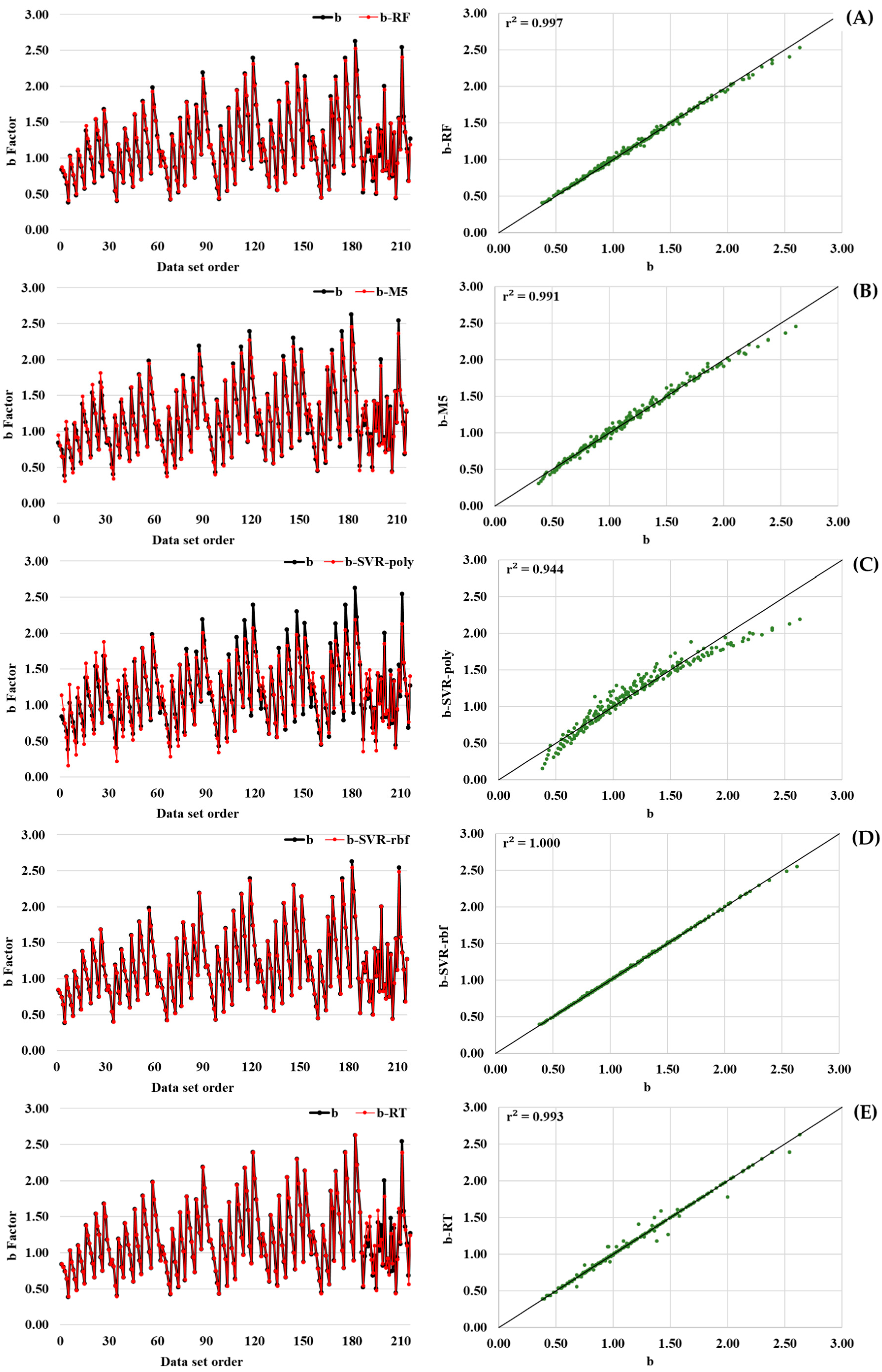
Figure 1. Performance of eight models in testing stage: (A) RF, (B) M5, (C) SVR-poly, (D) SVR-rbf, (E) RT, (F) Frevert et al., (G) Allen & Pruitt, and (H) Ambas & Evanggelos.
Atmosphere 13 01536 g001aAtmosphere 13 01536 g001b
Figure 2. Taylor diagram for seven models in the testing stage.
Atmosphere 13 01536 g002
Figure 3. The explicit equation rule set obtained from M5.
Atmosphere 13 01536 g003
Table 2. Summary of the optimal hyper-parameters for soft computing models.
Hyper-ParameterRFM5SVR-polySVR-rbfRT
ValueSensitiveValueSensitiveValueSensitiveValueSensitiveValueSensitive
numIteration300yes--------
batchSize 100no100no----100no
numExecutionSlots1no--------
minNumInstances--4yes------
numDecimalPLaces--4no----2no
buildRegressionTree--FALSEyes------
complexity----0.8yes1.0yes--
exponent----1.0yes --
gamma------1.0yes--
minNum--------1.0yes
numFolds--------0yes
minVarianceProp --------0.001yes
RRSE12.1411.4624.212.3724.23
Table 3. Statistical indices comparison in a testing stage for the present and previous studies.
Statistical
Indices
Present StudyPrevious Studies
RFM5SVR-polySVR-rbfRTFrevert et al. (1983)Allen & Pruitt
(1991)
Ambas &
Evanggelos (2010)
RBF Network
MARE (%)1.812.967.520.491.193.071.695.990.34
MXARE (%)8.119.258.75.017.614.411.841.11.8
NE > 2%80116171725126641410
DEV (%)1.622.978.000.553.162.721.687.220.31
r20.9970.9910.9441.0000.9930.9890.9980.9621.000
Table 4. The monthly climatological variables.
MonthsClimatological Variables
T (°C)RHmin (%)U2 (m/s)n/NPA
Feb.1.8651.400.2760.240−1.407
Mar.8.3501.890.3660.270−1.561
Apr.10.5501.650.3900.300−1.585
May12.7611.600.3110.330−1.459
Jun.20.6450.770.6360.347−1.853
Jul.21.4551.170.5350.337−1.709
Aug.19.6561.000.5100.310−1.679
Sep.17.9431.250.6260.280−1.851
Oct.11.6551.440.3230.250−1.497
Nov.7.8631.340.2380.220−1.377
Table 5. The results of the soft computing models, a table interpolation method, and the regression-based models applied for the b-factor estimation.
Months b
Frevert et al.
(1983)
Allen & Pruitt (1991)Ambas &
Evanggelos (2010)
Table
Interpolation
[25]
RBF [25]RFM5SVR-polySVR-rbfRT
Feb.0.7790.7880.8030.8210.8230.8460.8440.8230.8230.823
Mar.0.9650.9770.9891.0111.0121.0021.0081.0121.0121.012
Apr.0.9750.9810.9931.0161.0171.0001.0001.0171.0221.020
May0.8360.8460.8600.8860.8840.8880.9090.8830.8840.884
Jun.1.1751.1361.1491.1621.1651.1741.1411.1741.1651.165
Jul.1.0301.0151.0251.0471.0531.0471.0881.0521.0541.053
Aug.0.9980.9820.9941.0171.0221.0351.0381.0211.0221.020
Sep.1.2031.1791.1851.1991.2021.2021.1971.2021.2021.202
Oct.0.8810.8890.9030.9280.9300.9400.9000.9290.9300.930
Nov.0.7640.7750.7910.8130.8110.8310.7950.8120.8180.811
Table 6. The difference between the b-factor obtained from various methods and a table interpolation method.
Months Difference of b-Factor
Frevert et al.
(1983)
Allen & Pruitt (1991)Ambas &
Evanggelos (2010)
Table
Interpolation
[25]
RBF [25]RFM5SVR-polySVR-rbfRT
Feb.−0.042−0.033−0.0180.0000.0020.0250.0230.0020.0020.002
Mar.−0.046−0.034−0.0220.0000.001−0.009−0.0030.0010.0010.001
Apr.−0.041−0.035−0.0230.0000.001−0.016−0.0160.0010.0060.004
May−0.050−0.040−0.0260.000−0.0020.0020.023−0.003−0.002−0.002
Jun.0.013−0.026−0.0130.0000.0030.012−0.0210.0120.0030.003
Jul.−0.017−0.032−0.0220.0000.0060.0000.0410.0050.0070.006
Aug.−0.019−0.035−0.0230.0000.0050.0180.0210.0040.0050.003
Sep.0.004−0.020−0.0140.0000.0030.003−0.0020.0030.0030.003
Oct.−0.047−0.039−0.0250.0000.0020.012−0.0280.0010.0020.002
Nov.−0.049−0.038−0.0220.000−0.0020.018−0.018−0.0010.005−0.002
Table 7. Estimated Monthly Reference evapotranspiration (ETo).
Months ETo (mm/month)
Frevert et al.
(1983)
Allen & Pruitt (1991)Ambas &
Evanggelos (2010)
Table Interpolation
[25]
RBF
[25]
RFM5SVR-polySVR-rbfRT
Feb.7.58.18.910.010.211.511.410.210.210.2
Mar.48.149.350.652.752.851.852.452.852.852.8
Apr.66.166.968.371.071.169.169.171.171.771.4
May74.375.777.781.481.181.784.781.081.181.1
Jun.159.8152.7155.0157.4157.9159.6153.5159.6157.9157.9
Jul.140.4137.6139.6143.6144.8143.6151.3144.6145.0144.8
Aug.112.3109.7111.8115.5116.3118.5119.0116.2116.3116.0
Sep.109.8106.5107.3109.3109.7109.7109.0109.7109.7109.7
Oct.45.646.447.950.550.751.747.550.650.750.7
Nov.17.818.619.921.621.423.020.221.522.021.4
Yearly781.7771.5786.9813.0816.0820.2818.2817.1817.3816.0
Yearly
Difference (%)
−3.9−5.1−3.20.00.40.90.60.50.50.4
Publisher’s Note: MDPI stays neutral with regard to jurisdictional claims in published maps and institutional affiliations.