
A Multi-Year Study of GOES-13 Droplet Effective Radius Retrievals for Warm Clouds over South America and Southeast Pacific

 , and
, and
Abstract
1. Introduction
2. Materials and Methods
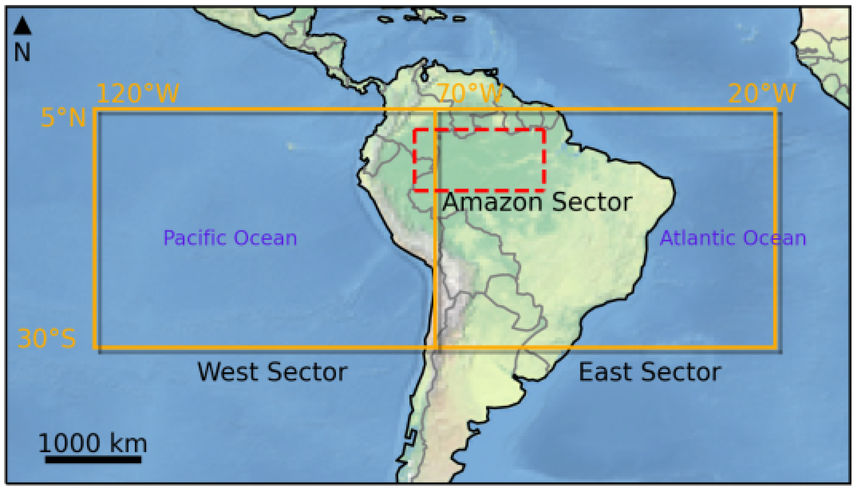
2.1. Spatial–Temporal Domain and Datasets
2.2. GOES-13 and Phase Retrievals
2.3. MODIS Match Up and Spatial–Temporal Comparison Strategy
2.4. Aircraft In Situ Match Up and Comparison Strategy
3. Results
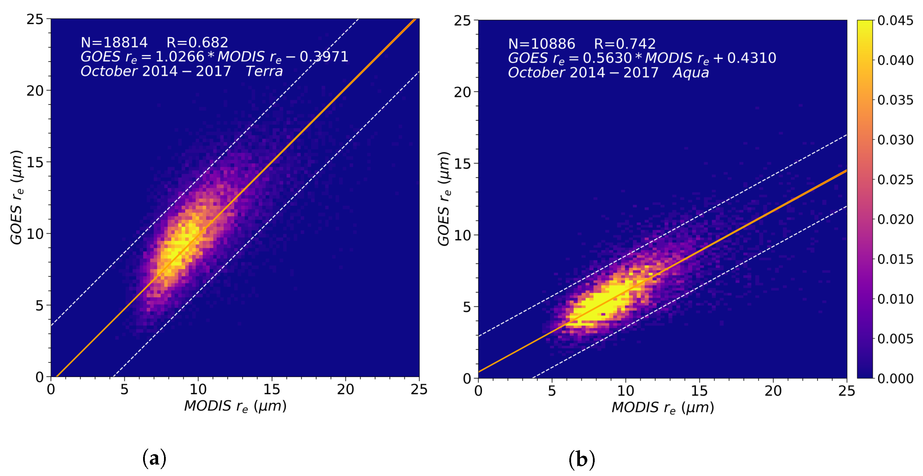
3.1. GOES-13 Imager and MODIS Direct Matchup Results
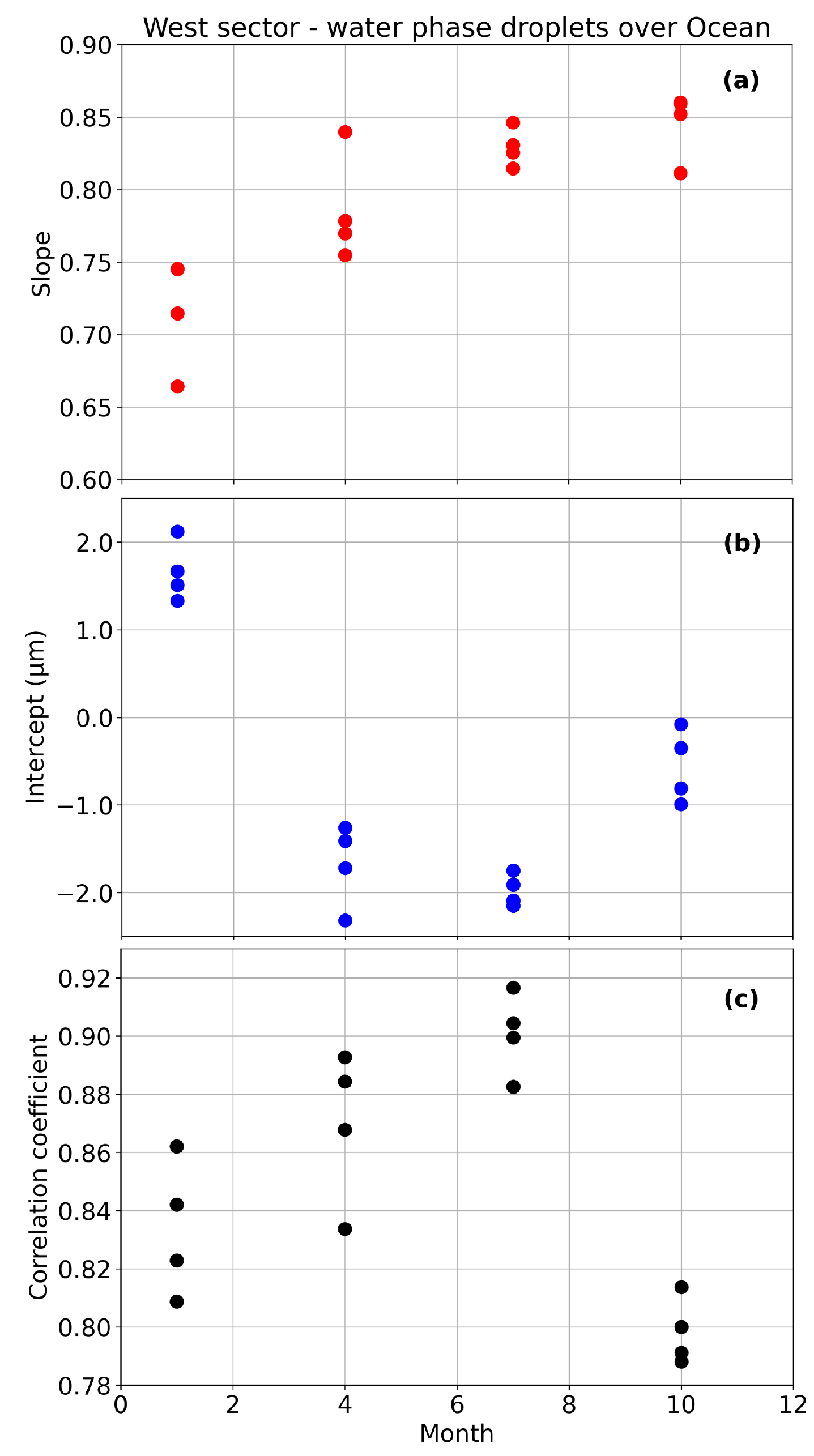
3.2. GOES-13 Monthly Matchups for MODIS Terra and Aqua
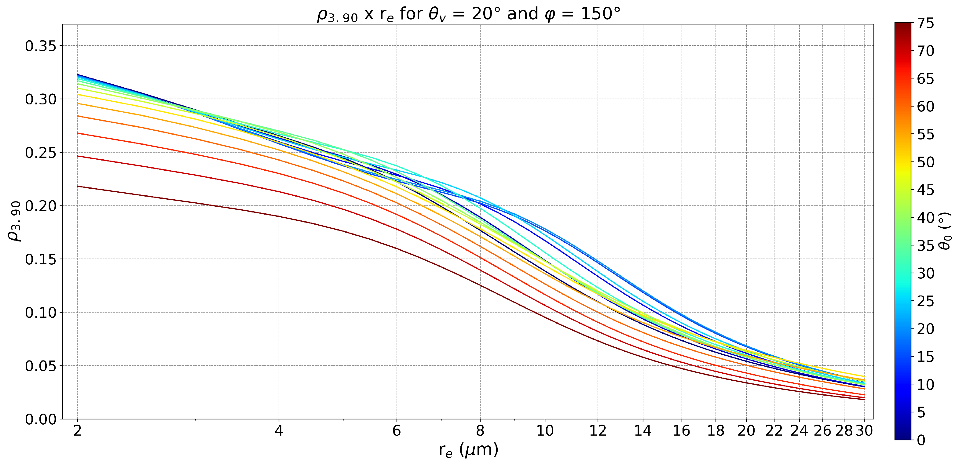
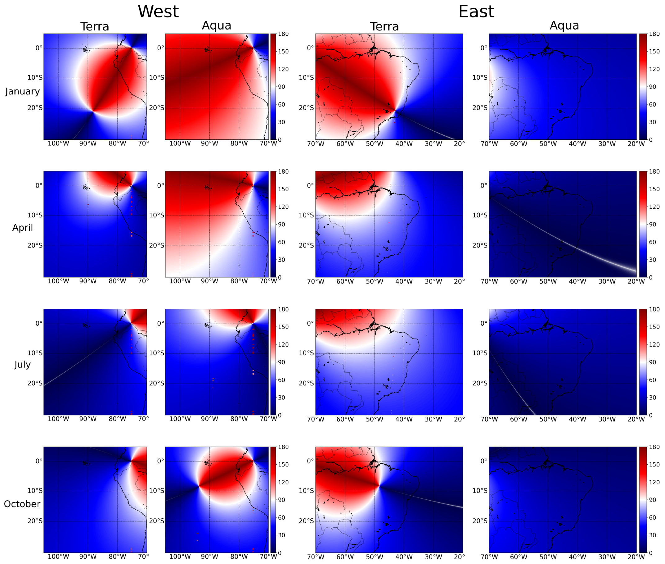
3.3. Assessing GOES-13 Sensitivity to Illumination and Observation Geometries
3.4. GOES-13 In Situ Aircraft Matchups during GoAmazon
4. Discussion
5. Conclusions
Author Contributions
Funding
Data Availability Statement
Acknowledgments
Conflicts of Interest
References
- Nakajima, T.; King, M.D. Determination of the Optical Thickness and Effective Particle Radius of Clouds from Reflected Solar Radiation Measurements. Part I: Theory. J. Atmos. Sci. 1990, 47, 1878–1893. [Google Scholar] [CrossRef]
- Twomey, S. The Influence of Pollution on the Shortwave Albedo of Clouds. J. Atmos. Sci. 1977, 34, 1149–1152. [Google Scholar] [CrossRef]
- Albrecht, B.A. Aerosols, Cloud Microphysics, and Fractional Cloudiness. Science 1989, 245, 1227–1230. [Google Scholar] [CrossRef] [PubMed]
- Rosenfeld, D. TRMM observed first direct evidence of smoke from forest fires inhibiting rainfall. Geophys. Res. Lett. 1999, 26, 3105–3108. [Google Scholar] [CrossRef]
- Wang, H.; Dai, T.; Zhao, M.; Goto, D.; Bao, Q.; Takemura, T.; Nakajima, T.; Shi, G. Aerosol Effective Radiative Forcing in the Online Aerosol Coupled CAS-FGOALS-f3-L Climate Model. Atmosphere 2020, 11, 1115. [Google Scholar] [CrossRef]
- Forster, P.; Storelvmo, T.; Armour, K.; Collins, W.; Dufresne, J.L.; Frame, D.; Lunt, D.; Mauritsen, T.; Palmer, M.; Watanabe, M.; et al. Chapter 7: The Earth’s energy budget, climate feedbacks, and climate sensitivity. In Climate Change 2021: The Physical Science Basis. Contribution of Working Group I to the Sixth Assessment Report of the Intergovernmental Panel on Climate Change; Open Access Victoria University of Wellington: Wellington, New Zealand, 2021. [Google Scholar] [CrossRef]
- Feingold, G.; Eberhard, W.L.; Veron, D.E.; Previdi, M. First measurements of the Twomey indirect effect using ground-based remote sensors: Surface remote sensing of the indirect effect. Geophys. Res. Lett. 2003, 30. [Google Scholar] [CrossRef]
- Zheng, X.; Xi, B.; Dong, X.; Logan, T.; Wang, Y.; Wu, P. Investigation of aerosol–cloud interactions under different absorptive aerosol regimes using Atmospheric Radiation Measurement (ARM) southern Great Plains (SGP) ground-based measurements. Atmos. Chem. Phys. 2020, 20, 3483–3501. [Google Scholar] [CrossRef]
- Sena, E.T.; McComiskey, A.; Feingold, G. A long-term study of aerosol–cloud interactions and their radiative effectat the Southern Great Plains using ground-based measurements. Atmos. Chem. Phys. 2016, 16, 11301–11318. [Google Scholar] [CrossRef]
- Hansen, J.E.; Travis, L.D. Light scattering in planetary atmospheres. Space Sci. Rev. 1974, 16, 527–610. [Google Scholar] [CrossRef]
- Platnick, S.; Meyer, K.G.; King, M.D.; Wind, G.; Amarasinghe, N.; Marchant, B.; Arnold, G.T.; Zhang, Z.; Hubanks, P.A.; Holz, R.E.; et al. The MODIS Cloud Optical and Microphysical Products: Collection 6 Updates and Examples From Terra and Aqua. IEEE Trans. Geosci. Remote Sens. 2017, 55, 502–525. [Google Scholar] [CrossRef]
- Dong, X.; Mace, G.G.; Minnis, P.; Smith, W.L.; Poellot, M.; Marchand, R.T.; Rapp, A.D. Comparison of Stratus Cloud Properties Deduced from Surface, GOES, and Aircraft Data during the March 2000 ARM Cloud IOP. J. Atmos. Sci. 2002, 59, 3265–3284. [Google Scholar] [CrossRef]
- McHardy, T.M.; Dong, X.; Xi, B.; Thieman, M.M.; Minnis, P.; Palikonda, R. Comparison of Daytime Low-Level Cloud Properties Derived From GOES and ARM SGP Measurements. J. Geophys. Res. Atmos. 2018, 123, 8221–8237. [Google Scholar] [CrossRef]
- Painemal, D.; Minnis, P.; Ayers, J.K.; O’Neill, L. GOES-10 microphysical retrievals in marine warm clouds: Multi-instrument validation and daytime cycle over the southeast Pacific: Marine clouds microphysics from GOES-10. J. Geophys. Res. Atmos. 2012, 117, 19212. [Google Scholar] [CrossRef]
- Painemal, D.; Spangenberg, D.; Smith, W.L., Jr.; Minnis, P.; Cairns, B.; Moore, R.H.; Crosbie, E.; Robinson, C.; Thornhill, K.L.; Winstead, E.L.; et al. Evaluation of satellite retrievals of liquid clouds from the GOES-13 imager and MODIS over the midlatitude North Atlantic during the NAAMES campaign. Atmos. Meas. Tech. 2021, 14, 6633–6646. [Google Scholar] [CrossRef]
- Kang, L.; Marchand, R.; Smith, W. Evaluation of MODIS and Himawari-8 Low Clouds Retrievals Over the Southern Ocean With In Situ Measurements From the SOCRATES Campaign. Earth Space Sci. 2021, 8, e01397. [Google Scholar] [CrossRef]
- King, N.J.; Bower, K.N.; Crosier, J.; Crawford, I. Evaluating MODIS cloud retrievals with in situ observations from VOCALS-REx. Atmos. Chem. Phys. 2013, 13, 191–209. [Google Scholar] [CrossRef]
- Painemal, D.; Zuidema, P. Assessment of MODIS cloud effective radius and optical thickness retrievals over the Southeast Pacific with VOCALS-REx in situ measurements: MODIS VALIDATION DURING VOCALS-REx. J. Geophys. Res. Atmos. 2011, 116. [Google Scholar] [CrossRef]
- Noble, S.R.; Hudson, J.G. MODIS comparisons with northeastern Pacific in situ stratocumulus microphysics. J. Geophys. Res. Atmos. 2015, 120, 8332–8344. [Google Scholar] [CrossRef]
- Zhang, Z.; Dong, X.; Xi, B.; Song, H.; Ma, P.; Ghan, S.J.; Platnick, S.; Minnis, P. Intercomparisons of marine boundary layer cloud properties from the ARM CAP-MBL campaign and two MODIS cloud products. J. Geophys. Res. Atmos. 2017, 122, 2351–2365. [Google Scholar] [CrossRef]
- Benas, N.; Meirink, J.F.; Stengel, M.; Stammes, P. Sensitivity of liquid cloud optical thickness and effective radius retrievals to cloud bow and glory conditions using two SEVIRI imagers. Atmos. Meas. Tech. 2019, 12, 2863–2879. [Google Scholar] [CrossRef]
- Grosvenor, D.P.; Wood, R. The effect of solar zenith angle on MODIS cloud optical and microphysical retrievals within marine liquid water clouds. Atmos. Chem. Phys. 2014, 14, 7291–7321. [Google Scholar] [CrossRef]
- Horváth, Á.; Seethala, C.; Deneke, H. View angle dependence of MODIS liquid water path retrievals in warm oceanic clouds. J. Geophys. Res. Atmos. 2014, 119, 8304–8328. [Google Scholar] [CrossRef]
- Liang, L.; Di Girolamo, L.; Sun, W. Bias in MODIS cloud drop effective radius for oceanic water clouds as deduced from optical thickness variability across scattering angles. J. Geophys. Res. Atmos. 2015, 120, 7661–7681. [Google Scholar] [CrossRef]
- Marshak, A.; Platnick, S.; Várnai, T.; Wen, G.; Cahalan, R.F. Impact of three-dimensional radiative effects on satellite retrievals of cloud droplet sizes. J. Geophys. Res. 2006, 111, D09207. [Google Scholar] [CrossRef]
- Zhang, Z.; Ackerman, A.S.; Feingold, G.; Platnick, S.; Pincus, R.; Xue, H. Effects of cloud horizontal inhomogeneity and drizzle on remote sensing of cloud droplet effective radius: Case studies based on large-eddy simulations: Heterogeneity and drizzle effect on effective radius retrieval. J. Geophys. Res. Atmos. 2012, 117, 19208. [Google Scholar] [CrossRef]
- Werner, F.; Zhang, Z.; Wind, G.; Miller, D.J.; Platnick, S. Quantifying the Impacts of Subpixel Reflectance Variability on Cloud Optical Thickness and Effective Radius Retrievals Based On High-Resolution ASTER Observations. J. Geophys. Res. Atmos. 2018, 123, 4239–4258. [Google Scholar] [CrossRef]
- Kato, S.; Hinkelman, L.M.; Cheng, A. Estimate of satellite-derived cloud optical thickness and effective radius errors and their effect on computed domain-averaged irradiances. J. Geophys. Res. 2006, 111, D17201. [Google Scholar] [CrossRef]
- Zhang, Z.; Werner, F.; Cho, H.M.; Wind, G.; Platnick, S.; Ackerman, A.S.; Di Girolamo, L.; Marshak, A.; Meyer, K. A framework based on 2-D Taylor expansion for quantifying the impacts of subpixel reflectance variance and covariance on cloud optical thickness and effective radius retrievals based on the bispectral method: Subpixel impact on retrievals. J. Geophys. Res. Atmos. 2016, 121, 7007–7025. [Google Scholar] [CrossRef]
- Vant-Hull, B.; Marshak, A.; Remer, L.A.; Li, Z. The Effects of Scattering Angle and Cumulus Cloud Geometry on Satellite Retrievals of Cloud Droplet Effective Radius. IEEE Trans. Geosci. Remote Sens. 2007, 45, 1039–1045. [Google Scholar] [CrossRef]
- Platnick, S. Vertical photon transport in cloud remote sensing problems. J. Geophys. Res. Atmos. 2000, 105, 22919–22935. [Google Scholar] [CrossRef]
- Weinreb, M.; Jamieson, M.; Fulton, N.; Chen, Y.; Johnson, J.X.; Bremer, J.; Smith, C.; Baucom, J. Operational calibration of Geostationary Operational Environmental Satellite-8 and -9 imagers and sounders. Appl. Opt. 1997, 36, 6895. [Google Scholar] [CrossRef] [PubMed]
- Kaufman, Y.J.; Nakajima, T. Effect of Amazon Smoke on Cloud Microphysics and Albedo-Analysis from Satellite Imagery. J. Appl. Meteorol. 1993, 32, 729–744. [Google Scholar] [CrossRef]
- Platnick, S.; Fontenla, J.M. Model Calculations of Solar Spectral Irradiance in the 3.7-m Band for Earth Remote Sensing Applications. J. Appl. Meteorol. Climatol. 2008, 47, 124–134. [Google Scholar] [CrossRef]
- Emde, C.; Buras-Schnell, R.; Kylling, A.; Mayer, B.; Gasteiger, J.; Hamann, U.; Kylling, J.; Richter, B.; Pause, C.; Dowling, T.; et al. The libRadtran software package for radiative transfer calculations (version 2.0.1). Geosci. Model Dev. 2016, 9, 1647–1672. [Google Scholar] [CrossRef]
- Correia, A.L.; Sena, E.T.; Silva Dias, M.A.F.; Koren, I. Preconditioning, aerosols, and radiation control the temperature of glaciation in Amazonian clouds. Commun. Earth Environ. 2021, 2, 168. [Google Scholar] [CrossRef]
- Mendonça, M.M. Estudo de Propriedades de Nuvens no Contexto de Sensoriamento Remoto com satéLites Usando cóDigos de Transferência Radiativa. Mestrado em Física, Universidade de São Paulo, São Paulo, Brazil, 2017. [Google Scholar] [CrossRef]
- Baum, B.A.; Yang, P.; Heymsfield, A.J.; Platnick, S.; King, M.D.; Hu, Y.X.; Bedka, S.T. Bulk Scattering Properties for the Remote Sensing of Ice Clouds. Part II: Narrowband Models. J. Appl. Meteorol. 2005, 44, 1896–1911. [Google Scholar] [CrossRef]
- Maddux, B.C.; Ackerman, S.A.; Platnick, S. Viewing Geometry Dependencies in MODIS Cloud Products. J. Atmos. Ocean. Technol. 2010, 27, 1519–1528. [Google Scholar] [CrossRef]
- Martin, S.T.; Artaxo, P.; Machado, L.A.T.; Manzi, A.O.; Souza, R.A.F.; Schumacher, C.; Wang, J.; Andreae, M.O.; Barbosa, H.M.J.; Fan, J.; et al. Introduction: Observations and Modeling of the Green Ocean Amazon (GoAmazon2014/5). Atmos. Chem. Phys. 2016, 16, 4785–4797. [Google Scholar] [CrossRef]
- Machado, L.A.T.; Calheiros, A.J.P.; Biscaro, T.; Giangrande, S.; Silva Dias, M.A.F.; Cecchini, M.A.; Albrecht, R.; Andreae, M.O.; Araujo, W.F.; Artaxo, P.; et al. Overview: Precipitation characteristics and sensitivities to environmental conditions during GoAmazon2014/5 and ACRIDICON-CHUVA. Atmos. Chem. Phys. 2018, 18, 6461–6482. [Google Scholar] [CrossRef]
- Schmid, B.; Tomlinson, J.M.; Hubbe, J.M.; Comstock, J.M.; Mei, F.; Chand, D.; Pekour, M.S.; Kluzek, C.D.; Andrews, E.; Biraud, S.C.; et al. The DOE ARM Aerial Facility. Bull. Am. Meteorol. Soc. 2014, 95, 723–742. [Google Scholar] [CrossRef]
- Cecchini, M.A.; Machado, L.A.T.; Comstock, J.M.; Mei, F.; Wang, J.; Fan, J.; Tomlinson, J.M.; Schmid, B.; Albrecht, R.; Martin, S.T.; et al. Impacts of the Manaus pollution plume on the microphysical properties of Amazonian warm-phase clouds in the wet season. Atmos. Chem. Phys. 2016, 16, 7029–7041. [Google Scholar] [CrossRef]
- Beswick, K.M.; Gallagher, M.W.; Webb, A.R.; Norton, E.G.; Perry, F. Application of the Aventech AIMMS20AQ airborne probe for turbulence measurements during the Convective Storm Initiation Project. Atmos. Chem. Phys. 2008, 8, 5449–5463. [Google Scholar] [CrossRef]
- Platnick, S.; Valero, F.P.J. A Validation of a Satellite Cloud Retrieval during ASTEX. J. Atmos. Sci. 1995, 52, 2985–3001. [Google Scholar] [CrossRef]
- Chen, Y.; Chen, G.; Cui, C.; Zhang, A.; Wan, R.; Zhou, S.; Wang, D.; Fu, Y. Retrieval of the vertical evolution of the cloud effective radius from the Chinese FY-4 (Feng Yun 4) next-generation geostationary satellites. Atmos. Chem. Phys. 2020, 20, 1131–1145. [Google Scholar] [CrossRef]


| Cloudy Pixel Condition | Transmission Function |
|---|---|
| 300 K | |
| 200 K K | |
| 200 K | |
| ; KK | |
| K; K | |
| GOES-13 × Terra MODIS | GOES-13 × Aqua MODIS | |||||||||
|---|---|---|---|---|---|---|---|---|---|---|
| Sector | Surface | Month (2014–2017) | N | R | Slope | Intercept (m) | N | R | Slope | Intercept (m) |
| West | Ocean | January | 52,944 | 0.839 | 0.717 | 1.85 | 18,461 | 0.894 | 0.744 | 0.42 |
| April | 32,147 | 0.876 | 0.796 | −1.59 | 11,951 | 0.889 | 0.729 | −1.51 | ||
| July | 108,009 | 0.912 | 0.871 | −2.24 | 55,634 | 0.891 | 0.751 | −1.42 | ||
| October | 93,266 | 0.778 | 0.863 | −0.84 | 39,429 | 0.880 | 0.776 | −0.18 | ||
| East | Land | January | 54,181 | 0.796 | 0.965 | 1.38 | 20,514 | 0.802 | 0.576 | 1.00 |
| April | 39,680 | 0.742 | 0.919 | 0.69 | 18,207 | 0.781 | 0.549 | 0.02 | ||
| July | 32,823 | 0.791 | 1.172 | −2.82 | 19,544 | 0.835 | 0.706 | −1.12 | ||
| October | 18,814 | 0.682 | 1.027 | −0.40 | 10,886 | 0.742 | 0.563 | 0.43 | ||
| Amazon | Land | January | 6040 | 0.775 | 0.838 | 1.97 | 1841 | 0.723 | 0.562 | 1.81 |
| April | 2144 | 0.609 | 0.708 | 2.47 | 486 | 0.598 | 0.536 | 1.55 | ||
| July | 4522 | 0.759 | 0.847 | −0.14 | 1764 | 0.794 | 0.559 | 0.70 | ||
| October | 1410 | 0.625 | 0.777 | 1.97 | 347 | 0.626 | 0.599 | 1.13 | ||
Publisher’s Note: MDPI stays neutral with regard to jurisdictional claims in published maps and institutional affiliations. |
© 2022 by the authors. Licensee MDPI, Basel, Switzerland. This article is an open access article distributed under the terms and conditions of the Creative Commons Attribution (CC BY) license (https://creativecommons.org/licenses/by/4.0/).
Share and Cite
Correia, A.L.; Mendonça, M.M.; Nobrega, T.F.; Pugliesi, A.C.; Cecchini, M.A. A Multi-Year Study of GOES-13 Droplet Effective Radius Retrievals for Warm Clouds over South America and Southeast Pacific. Atmosphere 2022, 13, 77. https://doi.org/10.3390/atmos13010077
Correia AL, Mendonça MM, Nobrega TF, Pugliesi AC, Cecchini MA. A Multi-Year Study of GOES-13 Droplet Effective Radius Retrievals for Warm Clouds over South America and Southeast Pacific. Atmosphere. 2022; 13(1):77. https://doi.org/10.3390/atmos13010077
Chicago/Turabian StyleCorreia, Alexandre L., Marina M. Mendonça, Thiago F. Nobrega, Andre C. Pugliesi, and Micael A. Cecchini. 2022. "A Multi-Year Study of GOES-13 Droplet Effective Radius Retrievals for Warm Clouds over South America and Southeast Pacific" Atmosphere 13, no. 1: 77. https://doi.org/10.3390/atmos13010077
APA StyleCorreia, A. L., Mendonça, M. M., Nobrega, T. F., Pugliesi, A. C., & Cecchini, M. A. (2022). A Multi-Year Study of GOES-13 Droplet Effective Radius Retrievals for Warm Clouds over South America and Southeast Pacific. Atmosphere, 13(1), 77. https://doi.org/10.3390/atmos13010077