Mobile On-Road Measurements of Aerosol Optical Properties during MOABAI Campaign in the North China Plain

Abstract

We present the mapping at fine spatial scale of aerosol optical properties using a mobile laboratory equipped with LIDAR (Light Detection And Ranging), sun photometer and in situ instruments for performing on-road measurements. The mobile campaign was conducted from 9 May to 19 May 2017 and had the main objective of mapping the distribution of pollutants in the Beijing and North China Plain (NCP) region. The highest AOD (Aerosol Optical Depth) at 440 nm of 1.34 and 1.9 were recorded during two heavy pollution episodes on 18 May and 19 May 2017, respectively. The lowest Planetary Boundary Layer (PBL) heights (0.5–1.5 km) were recorded during the heavy pollution events, correlating with the highest AOD and southern winds. The transport of desert dust from the Gobi Desert was captured during the mobile measurements, impacting Beijing during 9–13 May 2017. Exploring the NCP outside Beijing provided datasets for regions with scarce ground measurements and allowed the mapping of high aerosol concentrations when passing polluted cities in the NCP (Baoding, Tianjin and Tangshan) and along the Binhai New Area. For the first time, we provide mass concentration profiles from the synergy of LIDAR, sun photometer and in situ measurements. The case study along the Binhai New Area revealed mean extinction coefficients of 0.14 ± 0.10 km⁻¹ at 532 nm and a mass concentration of 80 ± 62 μg/m³ in the PBL (<2 km). The highest extinction (0.56 km⁻¹) and mass concentrations (404 μg/m³) were found in the industrial Binhai New Area. The PM₁₀ and PM_2.5 fractions of the total mass concentration profiles were separated using the columnar size distribution, derived from the sun photometer measurements. This study offers unique mobile datasets of the aerosol optical properties in the NCP for future applications, such as satellite validation and air quality studies.

1. Introduction

The North China Plain (NCP) in north-eastern China is one of the most populated and polluted regions of China, where long-standing heavy aerosol pollution episodes frequently occur [1,2]. The region has undergone a rapid development of urbanization and industrialization, leading to a deterioration in the air quality [3] and it becoming one of the regions with the most severe air pollution in China. Some of the most polluted cities in China (Beijing, Baoding, Tianjin, Tangshan, Shijiazhuang) are located in the NCP and air pollution has become an important concern in this region [4,5,6]. The major contributor to air pollution is particulate matter (PM), mainly fine particulate matter (PM_2.5) emitted from fossil fuels, biomass burning and urban construction [7]. The NCP is also impacted by frequent dust storms in the spring [8], with studies showing an increase in dust presence in the north-eastern and north-western regions [9]. Regional transport plays an important role in urban air pollution. Both local and regional sources contribute to the air pollution in the NCP region, depending on the synoptic conditions, with desert dust being advected over the NCP when air flows are dominated by westerly winds [10] while fine particle pollution events occur with southern wind flow [1]. The measures taken through air pollution control policies show an improvement in air quality and a negative trend for PM_2.5 concentrations since 2013 [11,12]. Nonetheless, the pollution levels are still high in the NCP, especially during haze episodes, and exceed the air quality limits locally. The air quality guideline (AQG) levels for 24 h for PM_2.5 and PM₁₀, as defined by the World Health Organization (WHO), are 15 µg/m³ and 45 µg/m³, respectively, which are lower than those established by the Ministry of Ecology and Environment of the People’s Republic of China of 35–75 µg/m³ for PM_2.5 and 50–150 µg/m³ for PM₁₀. A number of investigations on the air pollution in the NCP have been conducted over the years using fixed observation sites, aircraft measurements, mobile laboratories, satellite data and air quality models. A review of these studies in the NCP is given in [6]. Nonetheless, the fixed observatories in the NCP are generally located in or around large cities, mostly around Beijing, so measurements are sparse in the region and cannot capture the spatial variability of the aerosol properties at a fine scale or the regional impact of heavy pollution events. For this, a mobile instrumented laboratory performing on-line measurements on roads is useful to rapidly identify the pollution sources at short time and spatial scales, to characterize their optical properties and to assess the regional impact of pollution events.

In this paper, we report the mobile measurements of aerosol optical properties, such as aerosol optical depth (AOD), Angstrom Exponent (AE), particle volume size distribution (VSD) and vertical profiles of aerosol extinction and mass concentration derived from a sun photometer, LIDAR (Light Detection and Ranging) and in situ observations in the Beijing and NCP area during the 9–19 May 2017 period, performed during movement with an instrumented van. For the first time, such mobile LIDAR, sun photometer and in situ observations are performed on-road in the North China Plain. The aerosol size distribution, scattering and absorption properties at the surface level were measured by in situ optical instruments. The columnar volume size distribution was derived from spectral AOD measurements from the mobile sun photometer, and the extinction and mass concentration profiles were derived from the mobile LIDAR measurements. The aerosol optical properties are reported for different pollution levels in the NCP and for a case study along the Tianjin coastal area.

2. Materials and Methods

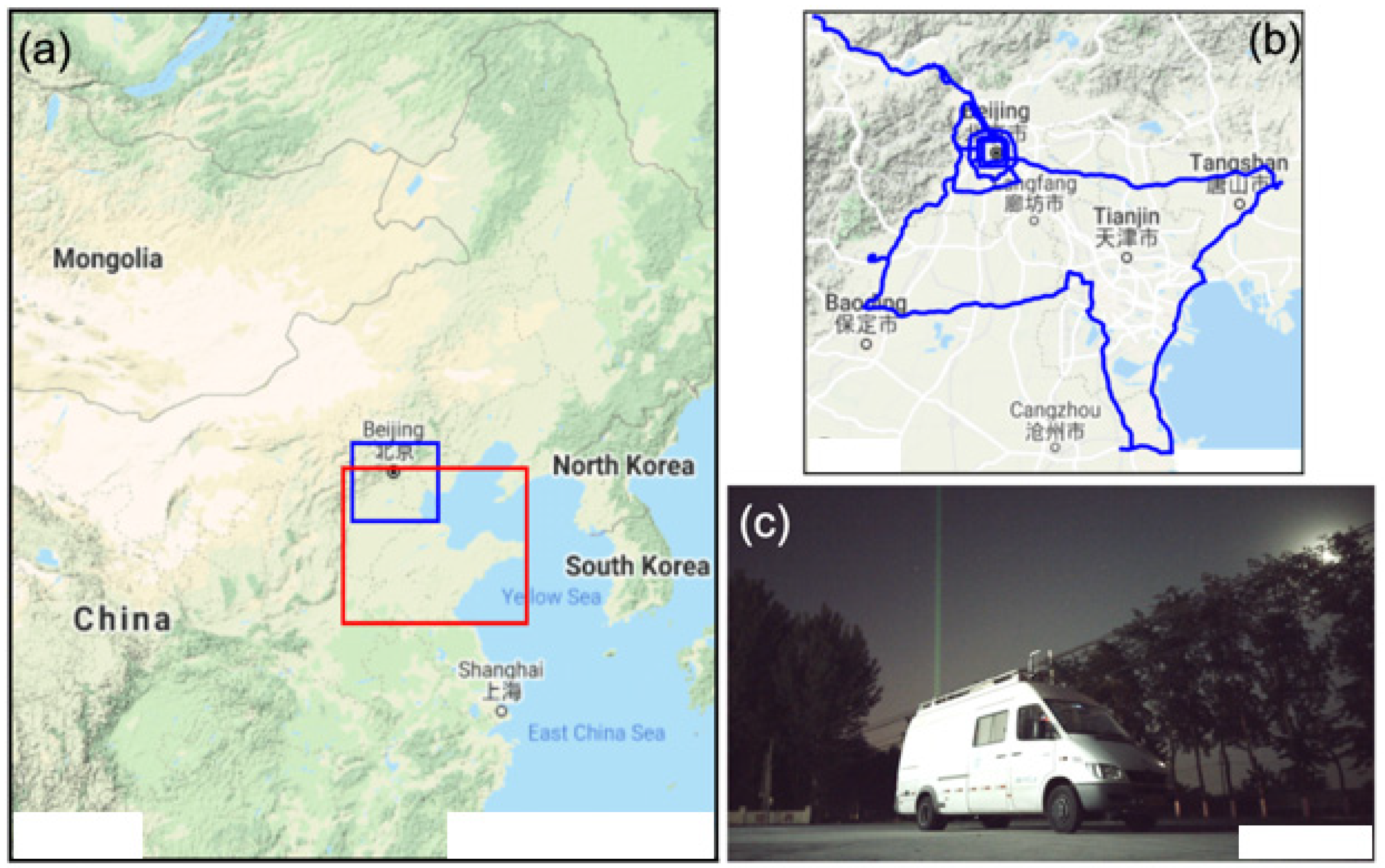
2.1. MOABAI Campaign

The Mobile Observation of Atmosphere by Vehicle-borne Aerosol Measurement Instruments (MOABAI) campaign was carried out from 9 to 19 May 2017 in the North China Plain. The transects of the mobile measurements and the mobile laboratory from the Institute of Atmospheric Physics (IAP) are shown in Figure 1. The mobile measurements were conducted on 10 days: 6 days in Beijing on the 4th, 5th and 6th ring roads by day and by night; and 4 days outside of Beijing, on the Beijing–Baoding–Tianjin (1), Tianjin—Tangshan (2), Tangshan—Beijing (3) and Beijing—Xiahuayuan (4) transects, as shown in Figure 1b.

2.2. Mobile Laboratory

The on-road mobile measurements were conducted with the IAP mobile laboratory Mercedes Benz 416 CDI diesel van, shown in Figure 1a,c (length 6.72 m, width 2.01 m, height 2.89 m, payload 5.6 tons). A power generator operated by the engine continuously supplied power when the van was on. An uninterrupted power supply was employed to regulate the voltage and frequency of electricity and supported all instruments for around 8 h when the engine was not switched on. A cooling system inside the van was used to maintain a constant temperature. The van was equipped with aerosol remote sensing and in situ instruments as well as real-time monitoring trace gas analyzers.

Table 1. Instruments set up in the IAP mobile laboratory during the MOABAI campaign. The aerosol properties in italic were derived from measurements using inversion algorithms.

Instrument	Make and Model	Wavelength (nm)	Temporal Resolution	Aerosol Physical/Chemical/Optical Properties	Uncertainty
Micro-pulse LIDAR	CE370, CIMEL	532	30 s	Vertical profile (Attenuated backscatter) (Extinction coefficient Mass concentration)	15% 25% 35–45%
PLASMA Sun Photometer	#650, LOA	340, 380, 440, 500, 675, 870, 940, 1020, 1640	10 s	Column-integrated optical properties (AOD, Angstrom Exponent, Precipitable Water) (Volume Size Distribution)	2% (VIS/NIR) 3% (UV) 10–20%
Nephelometer (3-λ)	Aurora 4000, Ecotech	450, 525, 635	30 s	Scattering coefficient	-
Aethalometer (7-λ)	AE33, Maggee Scientific	370, 470, 520, 590, 660, 880, 950	1 s	Absorption coefficient BC concentration	-
Optical Particle Counter (0.25–32 μm)	Sky-OPC model 1.129, GRIMM Aerosol Technik	655	6 s	Number concentration Number size distribution PM1, PM2.5, PM10 mass concentration	5%
NO–NO2–NOx analyser	42i, Thermo Electron	n/a	10 s	NO–NO2–NOx concentration	1%
SO2 analyser	43i, Thermo Electron	n/a	10 s	SO2 concentration	1%
O3 analyser	49i, Thermo Electron	n/a	20 s	O3 concentration	1%
Weather station	Airmar	n/a	1 s	Pressure, temperature, relative humidity, wind speed/direction	-

lists all instruments on board the mobile laboratory, the measured variables, temporal resolution and uncertainties. Only the measurements of the aerosol optical properties by remote sensing and in situ instruments are presented in this study. Gas phase parameters that were measured are not discussed in this study.

2.2.1. Micro-Pulse LIDAR

The CE370 CIMEL micro-pulse LIDAR and the Photomètre Léger Aéroporté pour la Surveillance des Masses d’Air (PLASMA) mobile sun photometer from the Mobile Aerosol Monitoring System (MAMS) payload [13] were transported and integrated on-site in the existing IAP van, which was already equipped with the in situ optical instruments and gas analyzers. The CE370 CIMEL micro-pulse LIDAR provided vertical profiles of the aerosols and clouds in the troposphere, from 200 m to around 12 km in altitude with a vertical resolution of 15 m. The LIDAR data quality was assured by following the Rayleigh fit protocol, as defined by the European Aerosol Research LIDAR Network (EARLINET) [14]. The uncertainties of the LIDAR measurements and the derived parameters have been presented previously [13] and are listed in Table 1.

2.2.2. Mobile Sun Photometer

The PLASMA sun photometer is the only existing mobile sun photometer that is able to track the sun when a vehicle is in motion. It meets the Aerosol Robotic Network (AERONET) standards and is included in the network, referenced as instrument #650. Compared to the CIMEL CE318 sun photometers in AERONET, the current PLASMA model performs only direct sun measurements. The instrument is calibrated by the Service National d’Observation, SNO PHOTONS/AERONET-EARLINET, a component of the Aerosols, Clouds and Trace Gases Research Infrastructure (ACTRIS) and the French component of AERONET. The PLASMA follows the AERONET calibration protocol for the reference master instrument and is also intercalibrated regularly against a master sun photometer from the PHOTONS network at the Observatoire de Haute Provence (OHP) in France before and after a field campaign. This allows for the checking of the instrument’s stability over time.

2.2.3. In Situ Optical Instruments

The in situ instruments consisted of a polar 3-λ nephelometer (Aurora 4000, Ecotech, Australia) [15], a 7-λ aethalometer (AE33, Maggee Scientific, Berkeley, CA, USA) [16], a Sky-OPC (11S, GRIMM Aerosol Technik, Ainring, Germany) and trace gas analyzers for NO₂, SO₂ and O₃. The aerosol was sampled using an isokinetic inlet facing forward. The sampled air was split into two flows. One flow was open and directly exposed to in-car air in order to remove the excess air and reduce the pressure in the instrument inlets. The tests showed that a van speed higher than 20 km/h could ensure that the open flow was large enough to prevent in-car air being sampled by the instruments downstream. The other flow passed through a Nafion dryer (MD-700, Perma Pure, Lakewood, NJ, USA) and then entered the nephelometer and aethalometer. The Sky-OPC had a separate isokinetic inlet, adapted for air velocities within a range of 16–25 m/s using a nozzle with a 1 mm opening (the speed of the van was approximately 60–90 km/h, when assuming the wind speed was 0). The gas analyzers were calibrated using standard gases before the campaign. The nephelometer was calibrated using air and R134 before the campaign. The flow of the aethalometer was checked before and after the campaign, and the deviations were within 4% of the setpoint.

2.2.4. Weather Station

Finally, the van was equipped with a weather station that measured the meteorological data (ambient pressure, temperature, relative humidity (RH) and wind speed/direction). The driving speed was kept at around 90 km/h (25 m/s), in order to cover as much distance as possible in the NCP region. For the in situ aerosol and gas measurements, the position of the inlets, at 3.3 m above the ground at the front of the van, was intended to reduce self-pollution from the van’s exhaust. The driving speed was also maintained at a constant speed, when possible, in order to provide a constant sampling flow rate and to reduce contamination from the van’s exhaust. The driving speed was higher than the normal wind speed, thereby the particles from the exhaust could not reach the inlet at the front of the vehicle during the measurements as a result of the wind from the back of the vehicle. The effects of self-pollution could be neglected for the remote sensing instruments as they measured either columnar variables or vertical profiles, starting from 200 m above ground level.

2.3. Methods for Retrieving Aerosol Properties

2.3.1. Extinction Profiles

A Klett–Fernald-based [17,18] backward inversion algorithm called BASIC [19,20] was used to invert the LIDAR data in synergy with the sun photometer data. The algorithm used the LIDAR overlap, range corrected signals (RCS) and the measured AOD to constrain the inversion. The optical aerosol properties derived were the extinction coefficient profiles, height-independent LIDAR ratio (LR), cloud, aerosol layers and Planetary Boundary Layer (PBL) heights. The algorithm’s description and applications to real data have been shown previously [13,20,21,22]. The sources of the uncertainties have been discussed in [13] and the uncertainty on the extinction profiles was 25%. In situ measurements were used to constrain the extinction profiles in the LIDAR blind zone (0–200 m). The scattering and absorption coefficients measured by the nephelometer and the aethalometer, respectively, were used to compute the extinction coefficients at surface level and a linear interpolation was applied between the LIDAR-derived extinction value at 200 m and the extinction measured in situ at surface level. Care needed to be taken with in situ measurements, as they provide the optical properties of dry particles and not those of ambient conditions as provided by the LIDAR. Some aerosols take in water and the effect of the RH is rather constant up to 70%, but a sharp increase in the scattering and extinction coefficients has been shown for RH > 70% [23,24]. The scattering coefficients were corrected for the RH effect following Equation (1) [25]:

$${\mathsf{\sigma }}_{\mathrm{sca},\mathrm{wet}}=\mathrm{f}\left(\mathrm{RH}\right){\mathsf{\sigma }}_{\mathrm{sca},\mathrm{dry}}$$

(1)

where ${\mathsf{\sigma }}_{\mathrm{sca},\mathrm{dry}}$ is the scattering coefficient of the dry particles measured by the nephelometer and $\mathrm{f}\left(\mathrm{RH}\right)$ is the aerosol hygroscopic growth factor, defined by the empirical Equation (2) [25]:

$$\mathrm{f}\left(\mathrm{RH}\right)=1+\mathrm{a}(\mathrm{RH}/{100)}^{\mathrm{b}}$$

(2)

where a and b are the fitting parameters for specific aerosol types, as found in the literature. The values used for this case study will be discussed in the dedicated section. For measurements when the RH > 40%, a correction was applied using the RH measured by the weather station on the roof of the mobile platform. The aerosol absorption coefficients at 520 nm were obtained from the aethalometer measurements, using a multiple scattering correction factor of 1.238 that was obtained in a comparison study in Beijing between the aethalometer and a 3-wavelength Photoacoustic Soot Spectrometer (PASS-3, Droplet Measurement Technologies, Boulder, CO, USA).

2.3.2. Columnar Volume Size Distribution

We used the Generalized Retrieval of Atmosphere and Surface Properties (GRASP) [26,27,28] (https://www.grasp-open.com/ (accessed on 30 November 2021)) algorithm to retrieve the columnar aerosol volume size distribution (VSD) from the spectral AOD measurements performed on-road with the PLASMA sun photometer. The GRASP application for direct sun measurements only, called GRASP-AOD, has been described previously [29,30]. The retrievals relied on a statistically optimized fitting of the sun photometer observations and the aerosol was assumed to be a mixture of spherical and non-spherical particles, with a defined sphere fraction and an assumed refractive index for the dominant aerosol type. The retrievals provided the six parameters describing the lognormal size distributions for the fine and coarse modes. The uncertainties of the retrieved size distributions lay within 5–10% for the fine mode and 10–20% for the coarse mode [29].

2.3.3. Mass Concentration Profiles

A Mass Extinction Efficiency (MEE) approach [31,32] was used to convert the aerosol extinction coefficient profiles, derived from the LIDAR–sun photometer–in situ synergy, into mass concentration profiles. The MEE related the total column extinction coefficient to the total mass concentration of the aerosols, computed for defined aerosol characteristics and defined by Equation (3) [32]:

$$\mathrm{MEE}=\frac{\mathsf{\pi }{{\displaystyle \int }}_{{\mathrm{r}}_{\min }}^{{\mathrm{r}}_{\max }}{\mathrm{r}}^2{\mathrm{Q}}_{\mathrm{ext}}\left(\mathrm{r},\mathrm{m},\mathsf{\lambda }\right)\mathrm{n}\left(\mathrm{r}\right)\mathrm{dr}}{\frac{4}{3}\mathsf{\pi }\mathsf{\rho }{{\displaystyle \int }}_{{\mathrm{r}}_{\min }}^{{\mathrm{r}}_{\max }}{\mathrm{r}}^3\mathrm{n}\left(\mathrm{r}\right)\mathrm{dr}} \left[\frac{1/\mathrm{m}}{{\mathrm{g}/\mathrm{m}}^3}\right]$$

(3)

where r is the particle radius, ${\mathrm{r}}_{\min }$ and ${\mathrm{r}}_{\max }$ are the limits of the particle size distribution, $\mathrm{n}\left(\mathrm{r}\right)$ is the number size distribution, ${\mathrm{Q}}_{\mathrm{ext}}$ is the Mie extinction efficiency computed for 532 nm, m is the complex refractive index and $\mathsf{\rho }$ is the particle density.

The MEE was computed assuming the particles were spherical and the following aerosol properties: columnar volume size distribution (VSD) retrieved with GRASP-AOD; refractive indices defined for the different aerosol types as found in the literature; and characteristic particle density for fine and coarse modes. The values used for the calculations are discussed further in the case study section. The aerosol mass concentration profiles, M(z), were derived using Equation (4):

$$\mathrm{M}\left(\mathrm{z}\right)=\frac{{\mathsf{\sigma }}_{\mathrm{ext}}\left(\mathrm{z}\right)}{\mathrm{MEE}} \left[\frac{\mathsf{\mu }\mathrm{g}}{{\mathrm{m}}^3}\right]$$

(4)

where ${\mathsf{\sigma }}_{\mathrm{ext}}\left(\mathrm{z}\right)$ is the aerosol extinction coefficient profile and MEE as previously defined.

This methodology has been applied previously for calculating volcanic ash mass concentration [19] and for mobile observations in France [13]. The uncertainty on the mass concentration profiles comes from the uncertainties on the extinction coefficient profiles, the aerosol size distribution, the assumed refractive index and the particle density. The overall uncertainty on the mass concentration profiles was estimated to be between 35% and 45%. The parameters used for computing the MEE and their uncertainty for the case study are presented in the results section.

3. Experimental Results

3.1. Overview of Aerosol Properties during MOABAI Campaign

The spatial variability of AOD at 440 nm and the Angstrom Exponent (AE) between 440 and 870 nm are shown in Figure 2. The maps show the variability of the aerosol optical properties at different scales: fine scale (5 × 3 km grid) of the city of Beijing (Figure 2a,g), medium scale (50 × 30 km grid) around the 5th ring road of Beijing (Figure 2b–c and h–i) and regional scale (200 × 250 km grid) in the Great Plain of North China (Figure 2e,k). The details of each mobile transect, the AOD, AE and PBL height ranges are summarized in

Table 2. Summary of mobile transects and aerosol properties observed during MOABAI campaign: AOD at 440 nm and Angstrom Exponent (AE) measured by the PLASMA sun photometer and PBL height derived from LIDAR measurements.

Mobile Transects	Date	AOD (440 nm) (Min–Max)	AE (440–870) (Min–Max)	PBL Height (km)
Beijing, 4th ring road	9 May 2017	0.62–0.84	0.67–0.93	1.7–2.2
Beijing, 5th ring road	11 May 2017	0.24–0.91	−0.03–1.12	1.5–3.6
Beijing, 5th and 6th ring road	13 May 2017	0.08–0.16	0.41–1.25	1.2–3.9
Beijing–Baoding–Tianjin (AB)	16 May 2017	0.2–0.7	0.38–2.32	0.3–1.7
Tianjin–Tangshan (BC)	17 May 2017	0.3–0.79	1–1.9	0.3–1.3
Tangshan–Beijing (CA)	18 May 2017	0.43–1.34	1.22–1.74	1–1.6
Beijing, 5th ring road	19 May 2017	1.47–1.9	1.21–1.51	0.5–1

.

Four mobile observations (9, 11, 13 and 19 May 2017) were conducted on Beijing’s 4th, 5th and 6th ring roads (Figure 2a–d,f–j,l) and three of the mobile observations were carried out outside of Beijing, in the NCP, on 16, 17 and 18 May 2017 (Figure 2e; Table 2). Five types of days were observed: (i) heavy pollution day (AOD of 0.72 ± 0.06) with desert dust contribution (AE of 0.79 ± 0.05) in Beijing (9 May 2017); (ii) desert dust episode (AE of 0.06 ± 0.08) with moderate aerosol loading (AOD of 0.37 ± 0.08) in Beijing (11 May 2017); (iii) clean day (AOD of 0.12 ± 0.02) but still with dust contribution (AE of 0.66 ± 0.05) in Beijing (13 May 2017); (iv) two moderate pollution days (AOD of 0.33 ± 0.05 and 0.45 ± 0.06, respectively) outside of Beijing (16 and 17 May 2017), consisting mainly of fine particles (AE of 1.08 ± 0.12 and 1.23 ± 0.1, respectively) but also with desert dust contribution at altitude; and (v) two heavy pollution days (AOD of 0.86 ± 0.2 and 1.69 ± 0.08, respectively), with a predominance of fine particles (AE of 1.41 ± 0.05 and 1.32 ± 0.05, respectively) in Beijing and the NCP (18 and 19 May 2017). Low AE values were recorded when north-westerly winds prevailed, due to Beijing and the NCP being downwind of the Asian dust storms from the Gobi Desert, while the highest AOD and AE measurements were recorded during regional heavy pollution episodes when air masses from the south were transported. For the moderate pollution and clean situations, there was a contribution of both fine and coarse particles, indicated by the AE values between those for the dust and fine particles episodes. For indication, the average AOD and AE measurements in Beijing during the spring are 0.8 and 1, respectively [8]. The lower AE measurements in the spring compared to other seasons show the impact of the dust episodes, as also observed during our mobile measurements during the MOABAI campaign.

Figure 3 shows the vertical distribution of the aerosol layers and clouds observed by the LIDAR during the MOABAI campaign. Most days had a clear sky, except for the afternoons of 16 and 19 May when cirrus clouds were present, explaining the lack of AOD measurements. The AOD at 440 nm and the PBL heights are also depicted in Figure 3, showing the correlation between the low PBL height and the high AOD values during the heavy pollution episodes.

The mean sea level pressure, and the wind direction and mean wind speed charts were analyzed and are presented in the Supplementary Material (Figures S1–S7). For 9 May 2017, the investigated area (Beijing) had a low-pressure tendency, which was being influenced by a well-developed depression situated over eastern Inner Mongolia (Figure S1). The wind direction showed that the air masses originated from the south. On 11 May 2017, the study area (Beijing) was at the junction between three high-pressure systems (Figure S2), one over southern Mongolia and the Gobi Desert, one over the Tibetan Plateau and one over the East China Sea. The pressure charts showed strong gradients from the W direction, where the desert is located, explaining the dust event identified in the measurements. The wind chart showed stronger winds over eastern Mongolia and a NW direction for the air masses passing over Beijing. On 13 May 2017, the study area (Beijing) had a low-pressure tendency (1008 hPa) under the influence of a low-pressure system located over North Korea, which pushed air to the region from a N-NW direction (Figure S3). On 16 May 2017, a high-pressure system could be observed over the Tibetan Plateau and the study area (Beijing–Baoding–Tianjin) was located in a slightly low-pressure area (1010 hPa) (Figure S4). A southern air flow with low wind speeds was observed over the region. On 17 May 2017, the area of interest (Tianjin–Tangshan) was located in a shallow low-pressure region (1008 hPa), with a southern air flow and low wind speeds (Figure S5). On 18 May 2017, the study area (Tangshan–Beijing) was located in a shallow low, at the junction between a depression over eastern Inner Mongolia and an anticyclone over the East China Sea (Figure S6). The air masses were transported from the south with low wind speeds. On 19 May 2017, the investigated area (Beijing) was located in a shallow low (1004 hPa) at the junction between two high-pressure systems, one over Irkutsk, Russia and one over the East China Sea (Figure S7). The air masses originated from the SW with low wind speeds.

Hybrid Single Particle Lagrangian Integrated Trajectory (HYSPLIT; [33]) back trajectories were performed for 72 h for all days, and the results are presented in the Supplementary Material (Figures S8 and S9). The air masses for the pollution day of 9 May 2017 originated from a S direction for the layers up to 2 km above ground level (AGL), while the aerosol layers at 3–4 km were transported from a NW direction, suggesting a desert dust contribution (also indicated by the lower AE values). The back trajectories for the dust episode (11 May 2017) showed that the air masses originated from a NW direction (Inner Mongolia), transporting dust from the Gobi Desert. For the clean day (13 May 2017), the air masses originated from the N, bringing clean air over Beijing with a small contribution of residual dust up to 4 km. The dust event during the 11–14 May 2017 period has also been discussed in [34]. Higher particle concentrations near the surface (increase in LIDAR backscatter signal) and lower PBL height compared to the rest of the transect were observed when passing polluted cities (Baoding, Tianjin, Tangshan) and industrial regions (Tianjin coastal area). The clear difference between the PBL heights of 13 May 2017 (3.5 km) and 16 May 2017 (0.5 km) is explained by the change in the synoptic conditions, as explained above. The lowest PBL heights (0.5–1.7 km) were recorded on the days with moderate and heavy fine particle pollution (16–19 May 2017), when air masses flowed from S and SW directions and passed over polluted cities in the NCP (Baoding, Shijiazhuang, Tianjin). The lofted aerosol layers observed at around 2 km AGL on 16 May 2017 and around 3 km on 17 May 2017 originated from N and NW directions, suggesting a desert dust contribution. For the heavy pollution days (18 and 19 May 2017), there was a clear correlation between the high AOD (0.86 and 1.69) and the low PBL heights (0.5–1.6 km). Our mobile measurements showed how the heavy pollution episodes impact the NCP region.

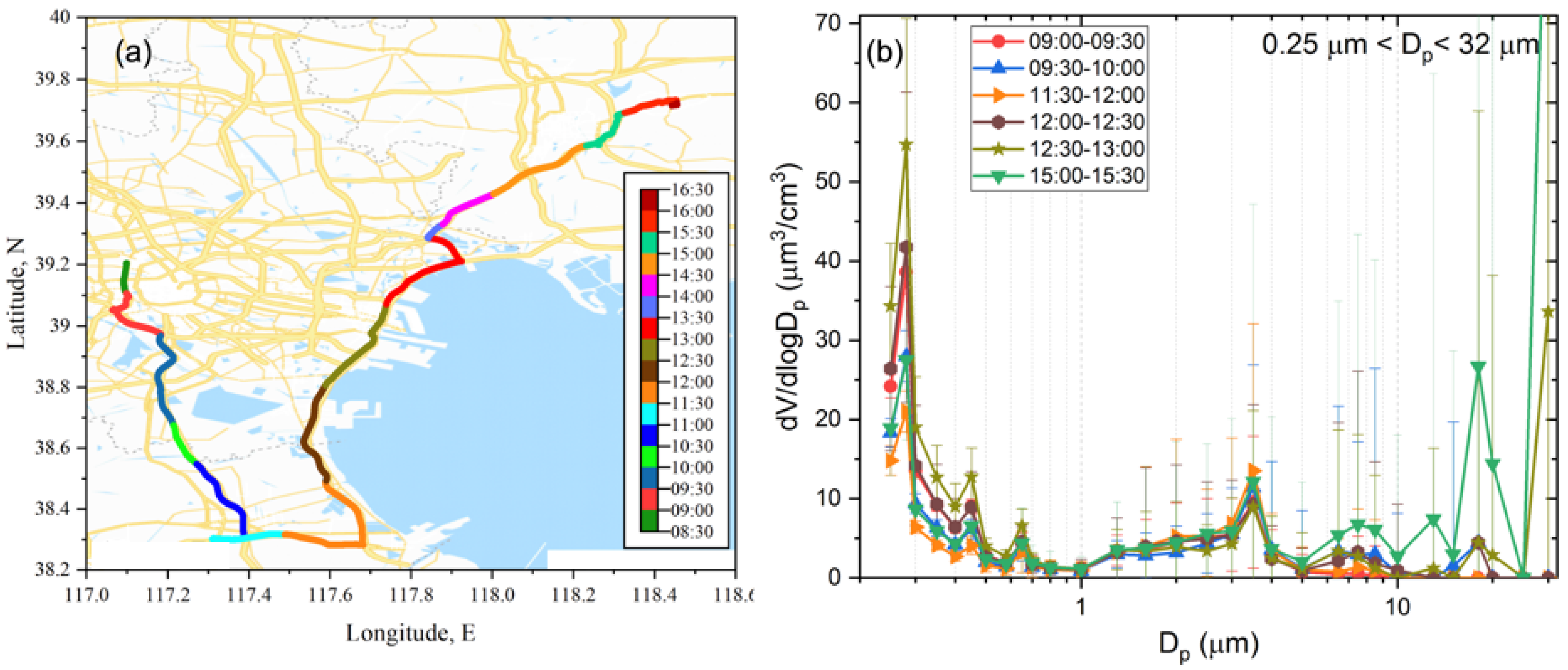
3.2. Case Study: Tianjin Coastal Area, 17 May 2017

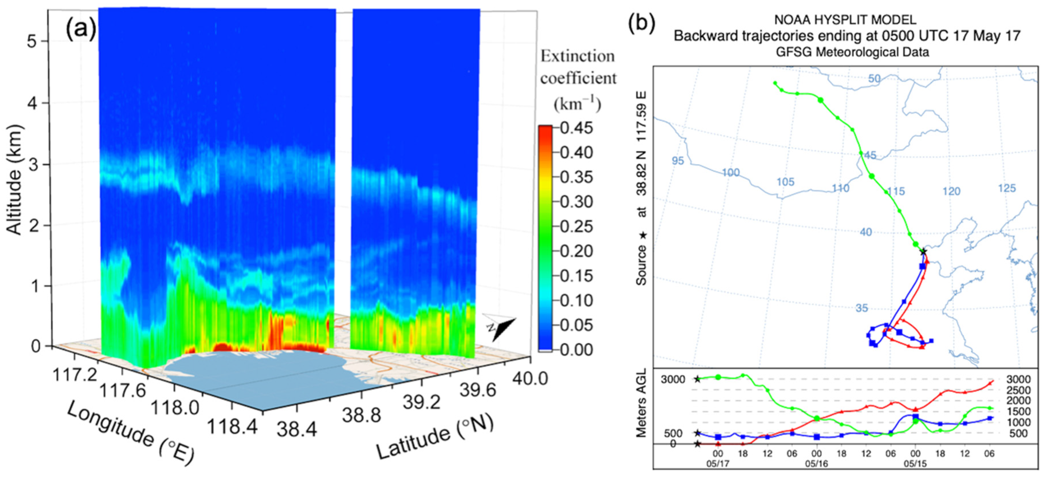
3.2.1. Study Area and Meteorological Conditions

The mobile transect and the local time of the measurements are presented in Figure 4a. The mobile observations started at 08:30 local time (UTC +08:00) from the city of Tianjin, headed south and then continued along the Bohai sea coast, passing through the industrialized Binhai New Area during the 12:00–13:30 time interval, and then headed northeast to Tangshan and stopped at Guye around 16:00 local time. The weather was fair with clear sky along the whole transect, ambient temperatures (T) of 24–30 °C and an RH in the 30–65% range, with a noticeable increase in RH along the coast (Figure 5c).

The Binhai New Area, about 60 km east of Tianjin city, is an important economic coastal area with considerable industrial activities, including the Tianjin port, the largest port in northern China and one of the largest ports in the world. The industry sectors vary from machinery factories, petrochemical manufacturing plants, automotive fitting factories and electronics facilities to sea salt production, shipbuilding and port activity and logistics. The area accounted for 271 industrial enterprises in 2012, resulting in heavy pollution in the region [35,36]. Both natural and anthropogenic sources, such as wind and soil erosion, sea salt, fossil-fuel combustion, vehicles emissions, construction activities, industrial processes and photochemical reactions, contribute to the particulate matter, resulting in a complex chemical composition of particles in this region [37]. It is an interesting study area, where the microphysical and optical properties of aerosols are not well-characterized, much less at a fine scale. The situation is even more complex in the spring because mineral dust transports occur frequently, adding to the anthropogenic pollution. One previous study presenting mobile LIDAR measurements has been conducted in Tianjin, during the different seasons of 2016 [38]. For their measurements in the spring, they found the maximum PM_2.5 concentrations near the port (200 μg/m³) and that the fine particles mainly concentrated below 0.5 km. Another study by [36] presents the variability of the microphysical and optical properties of aerosols as measured by sun photometers set up at three sites: urban, industrial and coastal areas of Tianjin. They found relatively high AOD values (0.71 ± 0.55) and moderately high AE values (1.09 ± 0.29) in the Tanggu region (near the coast of the Bohai Sea) in the spring. Nevertheless, this is the first time on-road mobile LIDAR, sun photometer and in situ measurements have been conducted in the Tianjin coastal area to map the variability of particle properties at a fine scale.

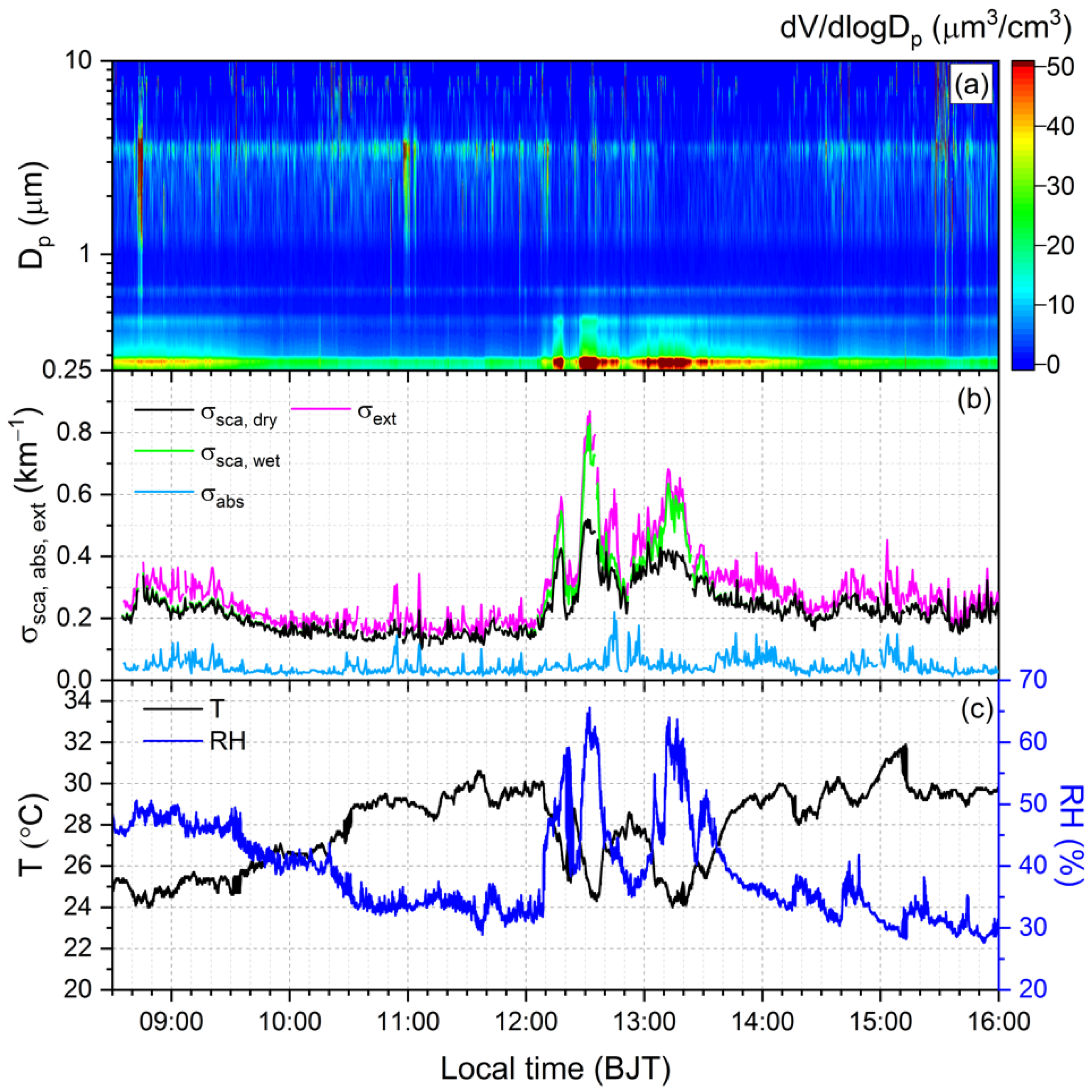
3.2.2. Particle Size Distribution at Surface Level

The mean volume size distributions measured by the Sky-OPC on 30 min road segments are presented in Figure 4b. In the fine mode, a peak centered below the 0.3 μm diameter was observed. In the supermicron range, a broad coarse mode was observed between 1 and 5 μm, with a distinct peak at 3.5 μm, all along the mobile transect, and the coarse mode centered at 7.5 μm. Super-coarse particles (>10 μm) are most probably re-suspended dust. The highest concentrations were observed at around 0.3 μm, showing that fine particle pollution is predominant at surface level. The sampled aerosols were a mixture of regional scale background aerosol and direct emissions from vehicles and industry. Both soot and secondary aerosol could contribute significantly to the submicron ambient aerosol. The study in [39] showed that the mass size distributions of both gasoline and diesel car emissions present a single mode with a peak at 0.2 μm. Studies on ship emissions have shown that particles with Dp < 0.3 μm dominate [40,41], which could also explain the increase in the fine mode centered at 0.3 μm when passing the Tianjin port. The explanation for the high increase in particle concentrations in the Binhai New Area is twofold. On the one hand, we passed a region with significantly higher pollution (industry emissions, intense traffic emissions), therefore higher particle concentrations. On the other hand, the increase in concentration could be an effect of particle growth in the presence of a higher RH. A clear correlation between the increase in RH and the increase in particle concentrations is seen in Figure 5. It has been shown that ship exhaust particles are highly hygroscopic in humid marine environments [42]. In our case, if particles smaller than 0.25 μm (the minimum diameter detectable by the Sky-OPC) increase in size due to water intake, they would be counted in the upper size bins, resulting in an increase in the number of particles in the upper size bins. An increase in concentration was observed for particles in the 0.25 < D_p < 0.8 μm range, meaning that, according to our hypotheses, these particles could be more hygroscopic and affected by water intake. Another interesting event depicted in Figure 5 is a clear episode of sea breeze, between 12:10 and 13:40, marked by a sudden increase in RH correlating with a drop in temperature. The sea breeze event suggests that sea salt was transported inland. Sea salt has a diameter of higher than 0.3 μm and is highly hygroscopic [43].

3.2.3. Aerosol Scattering and Absorption at Surface Level

The scattering (at 525 nm), absorption (at 520 nm) and extinction coefficients derived from the nephelometer and aethalometer measurements at surface level, as well as the T and RH monitored by the mobile weather station are presented in Figure 5. The aethalometer data was averaged on 30 s, and the RH correction to scattering coefficients (Equation (1) in Section 2.2) was applied to the nephelometer data in order to compute the ambient (wet) extinction coefficients at surface level. The a and b parameters in Equation (2) that were used for the RH correction were as follows: (i) a = 2.3 and b = 6.27 for the polluted aerosol type, according to [25], on the pollution segments of the mobile transect (08:40–12:00 and 13:30–16:00 local time); (ii) a = 3.26 and b = 3.27, following [44] for mixed urban–marine aerosols for the transects with sea salt intrusion (12:00–13:30 local time). The mean absorption, scattering (wet) and extinction at surface level were 0.05 ± 0.03 km⁻¹, 0.24 ± 0.11 km⁻¹ and 0.29 ± 0.12 km⁻¹, respectively, where the standard deviations represent the spatio-temporal variability along the route. An increase in both scattering and absorption coefficients was observed during the 12:00–13:30 time interval, when the scattering rose as high as 0.83 km⁻¹ and absorption as high as 0.22 km⁻¹. The mean SSA (Single Scattering Albedo) of the nephelometer (525 nm) and of the aethalometer (520 nm), computed using the measurements at two close wavelengths, for the whole transect was 0.84 ± 0.07.

Figure 6 shows the comparison between the in situ extinction coefficients at surface level and the LIDAR-derived extinction at a 210 m altitude (retrieved using a constant extrapolation in the inversion). Both dry and ambient (wet) extinction coefficients from in situ data are depicted in order to show the impact of the f(RH) correction on the segments where the RH > 50%. The LIDAR-derived extinction coefficients at a 210 m altitude demonstrated a very strong agreement with the in situ extinction at surface level. This good agreement between the LIDAR and in situ measurements validates the overlap correction used for the LIDAR data and shows that the assumption of homogeneity from the surface up to ~200 m of altitude (constant extrapolation) is reasonable for most of the mobile measurements. Significant differences were observed during the 12:00–13:30 time interval, probably due to the inhomogeneity of the aerosol distribution from the ground to a 200 m altitude. The extinction in this time interval measured by in situ instruments and corrected for RH effects was on average two times higher than the LIDAR-derived extinction. The differences could be explained by the significant increase in particle concentration and/or the change in aerosol type at surface level and not being “seen” by the LIDAR at a 200 m altitude. Secondly, the aerosol mixture assumption and the f(RH) correction applied to the nephelometer data could be not appropriate, resulting in an overestimation of the scattering coefficients. The LIDAR-derived extinction coefficients were highly correlated with the extinction measured by the in situ instruments, with an R² of 0.98, slope of 0.91 and RMSE (Root Mean Square Error) of 0.03 all along the transect, excluding the values in the 12:00–13:30 time interval. The correlation decreases when including the values in this time interval (R² of 0.9, slope of 0.53, RMSE of 0.08).

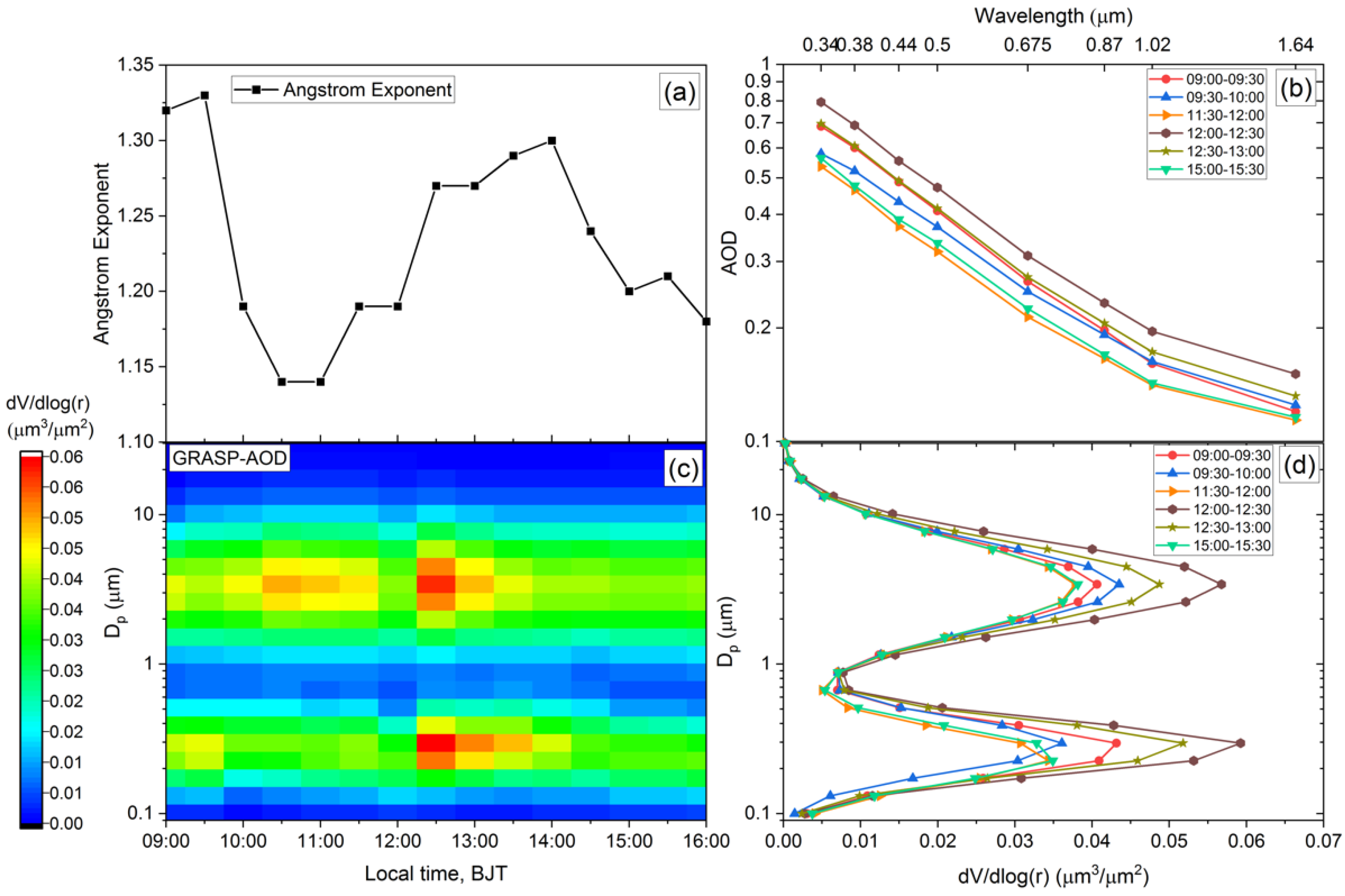
3.2.4. Columnar Volume Size Distribution

The total column aerosol volume size distributions (VSD) retrieved with the GRASP-AOD from the PLASMA photometer measurements are presented in Figure 7c,d. The spectral AOD (Figure 7b) and AE (Figure 7a) from the PLASMA measurements averaged on 30 min transects, as in Figure 4a, are also presented. The inversion requires the assumption of the refractive index and sphere fraction. Assumptions on the chemical composition of the aerosols were made based on the modes identified in the in situ-derived size distributions at surface level. An important contribution of elemental carbon (EC), organic carbon (OC) and sulphates was considered, indicated by the narrow fine mode peak at 0.3 μm, followed by a nitrate component (suggested by the coarse mode centered at 3.5 μm), a small contribution of dust at altitude (from the LIDAR data and backward trajectories analysis) and the sea salt contribution during the sea breeze event. According to a study conducted in Tianjin in the spring of 2009 [45], an average refractive index of 1.52–0.018i was found for an aerosol mixture that was similar to our case. For the retrievals, the assumption of spherical particles and a complex refractive index of 1.52–0.008i were used for most of the transects. A lower absorption (imaginary part) was considered, taking into account that desert dust was present in the free troposphere. For the part along the coast (12:00–13:30), a complex refractive index of 1.46–0.008i was used, considering the RH effect on the aerosols and the sea breeze event, following the results from [46] for the aerosol types in our case (fine particles that are predominantly sulphates) and for the maximum relative humidity (60–65%). The columnar size distributions present two modes, fine and coarse, centered at 0.3 μm and 3.4 μm diameters, respectively. The size distributions did not change significantly over the transects, except for an increase in both fine and coarse mode concentrations when reaching the polluted coastal region. The increase in the fine mode could be explained by the emissions from industry as well as the port, which could provide more primary aerosols in addition to the precursor gases for secondary aerosols. The increase in coarse mode along the coast could be explained by the sea salt intrusion during the sea breeze and the increase in nitrates in the high density industry region. A higher humidity could also result in hygroscopic growth and enhance the multi-phase chemistry. The change in particle size is shown by both the AE (Figure 7a) and VSD (Figure 7c). The highest AE values and slightly higher fine mode were observed in Tianjin. The decrease in the AE between 10:00 and 12:00 is explained by a lower contribution of fine particles than at Tianjin and an increase in the coarse mode in the VSD. Having fewer fine particles allowed us to better see the contribution of the desert dust layer to the AE in the free troposphere, followed by a decrease in the AE and an increase in coarse mode in the VSD between 10:00 and 11:30. In the coastal industrial region, the concentrations of both fine and coarse modes increased significantly and the AE increased, but was still lower than at Tianjin due to an important contribution of coarse mode. The columnar aerosol fine mode concentrations increased twofold during the 12:00–13:30 time interval, which was consistent with what was seen at surface level. Both in situ and columnar VSD measurements presented the same positions of the fine and coarse modes with diameters of 0.3 and 3.5 μm, respectively, which showed that the two major aerosol contributions were sulphates and black carbon (BC) in the fine mode and nitrates in the coarse mode.

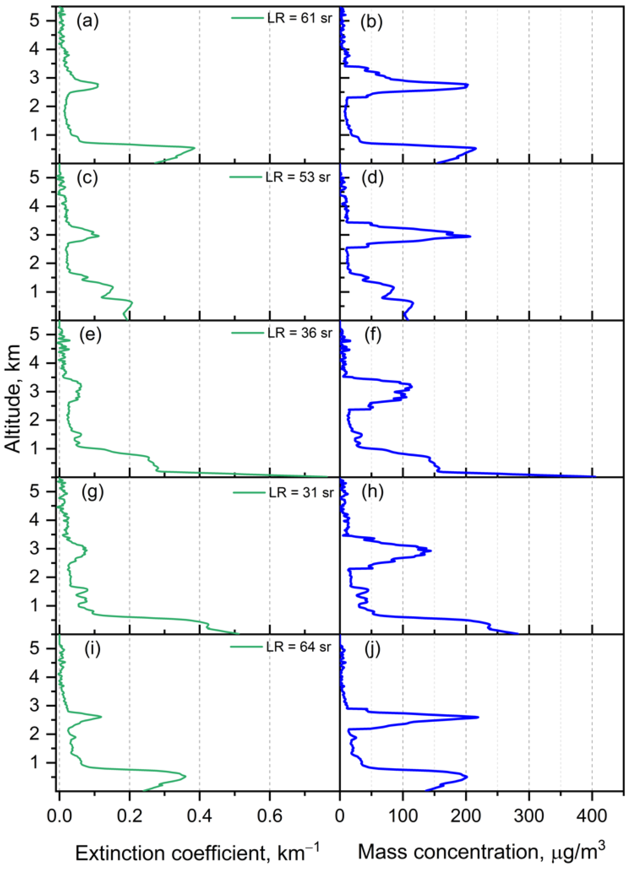
3.2.5. Extinction Coefficient Profiles

The spatial variability of the extinction coefficient profiles at 532 nm derived from the synergy of LIDAR, sun photometer and in situ measurements is presented in Figure 8a. The LIDAR Klett inversion, constrained by the AOD, was used to obtain the extinction profiles and the in situ instruments were constrained between surface level and a 200 m altitude. The mean extinction coefficient in the PBL, from surface level to about 2 km, was 0.14 ± 0.10 km⁻¹ along the whole transect from Tianjin to Tangshan, and the extinction reached a maximum of 0.56 km⁻¹ when passing the industrial coastal region.

Table 3. Mean aerosol extinction coefficients, LIDAR ratios (LRs) at 532 nm and mass concentrations in the PBL (0–2 km) for each time interval corresponding to the transect segments depicted in Figure 4a. The standard deviations correspond to the spatio-temporal variability within each transect segment.

Time Interval	${\mathsf{\sigma }}_{\mathbf{e}\mathbf{x}\mathbf{t}} \mathbf{\left(}{\mathbf{km}}^{\mathbf{-}\mathbf{1}}\mathbf{\right)}$	$\mathbf{L}\mathbf{R} \mathbf{\left(}\mathbf{sr}\mathbf{\right)}$	Mass Concentration (μg m−3)
08:40–09:00	0.14 ± 0.15	66 ± 10	80 ± 85
09:00–09:30	0.15 ± 0.15	59 ± 17	85 ± 82
09:30–10:00	0.13 ± 0.10	56 ± 10	75 ± 57
10:00–10:30	0.14 ± 0.07	52 ± 12	80 ± 41
10:30–11:00	0.13 ± 0.06	50 ± 11	74 ± 34
11:00–11:30	0.14 ± 0.06	43 ± 14	78 ± 33
11:30–12:00	0.1 ± 0.06	46 ± 14	57 ± 34
12:00–12:30	0.18 ± 0.09	40 ± 13	100 ± 50
12:30–13:00	0.16 ± 0.13	35 ± 12	88 ± 72
13:00–13:30	0.15 ± 0.13	39 ± 11	83 ± 71
13:30–14:00	0.15 ± 0.13	45 ± 11	87 ± 74
14:00–14:30	0.13 ± 0.11	42 ± 8	73 ± 60
14:30–15:00	0.13 ± 0.12	52 ± 12	71 ± 65
15:00–15:30	0.13 ± 0.12	47 ± 11	75 ± 66
15:30–16:00	0.13 ± 0.11	57 ± 14	71 ± 59

presents a summary of the derived properties, the mean extinction coefficients, LIDAR ratios and mass concentrations up to a 2 km altitude for each transect in Figure 4a. The standard deviations depict the spatio-temporal variability for each segment. The highest extinction coefficients were found near Tianjin city and along the industrial Binhai New Area. Some examples of extinction coefficients and mass concentration profiles along the route are depicted in Figure 9: at Tianjin (08:55); between Tianjin and the Binhai New Area (10:50); when crossing a salt pan (12:30); when crossing Tianjin port (13:00); and near Tangshan (15:20).

In the free troposphere, an elevated aerosol layer at 2.2–3.5 km was observed all along the mobile transect. The HYSPLIT back trajectories at 0 km, 0.5 km and 3 km, starting at 13:00 local time (05:00 UTC), illustrated in Figure 8b, show that the layer at about 3 km was transported from Inner Mongolia while the aerosols in the PBL had a local origin from the S-SE direction. The separation of the elevated dust layer (Figure 10) was done using the first derivative of the extinction profiles and by applying a threshold to separate the aerosol contributions above the PBL. The mean extinction coefficient of the dust layer was 0.05 ± 0.03 km⁻¹, with a maximum of 0.15 km⁻¹ at around 3 km at 10:30. The mean AOD at 532 nm of the dust layer was 0.06 ± 0.01, which represents 18–20% of the total measured AOD.

The variability of the height-independent extinction-to-backscatter ratio or LIDAR ratios (LRs) at 532 nm derived from the LIDAR–sun photometer inversions for each segment of the mobile transect is presented in Table 3. The standard deviations correspond to the spatio-temporal variability of each segment. The LR values decreased from 66 ± 10 sr at Tianjin to 35 ± 12 sr when crossing the Binhai New Area and then increased again to 57 ± 14 sr near Tangshan. The decrease in the LR indicates a change in the aerosol type. The LR around 60 sr, found at Tianjin and Tangshan, is characteristic of the urban-industrial aerosol type [47,48] while the LR around 40 sr corresponds to a marine aerosol type [48,49,50]. In our case, it was most probably a mixture of continental polluted and marine polluted aerosols (considering the sources along the coast), with a contribution of desert dust at altitude. The values found at Tianjin and Tangshan were consistent with a study conducted in Shangdianzi, located in the northern part of the North China Plain, where a mean LR of 60 sr was found [51]. The LRs found along the coast were similar to the values of 33 ± 14 sr, which were found at a site on the French coast [52], and of 40 sr, which was found on the Portuguese coast [53]. Both studies evidenced the presence of a sharp peak in the backscatter signal in the marine boundary layer, ranging between 200 and 650 m, where the air masses were coming from the direction of the sea, which is similar to what was observed in our case: a strong increase in the scattering coefficients below 200 m when reaching the coast. The sea salt presence in this region was clear, as salt pans are located in the places where the peaks were observed. The Tianjin municipality has a long history of sea salt exploitation and there were still two salt pans being exploited at that time according to [54], illustrating the coastal landscape map of Tianjin–Binhai New Area in 2013. The significant increase in the extinction coefficients seen below 200 m and the decrease in the columnar LR correspond to the time intervals when the mobile system was crossing the salt pans, and could be linked to a strong presence of sea salt.

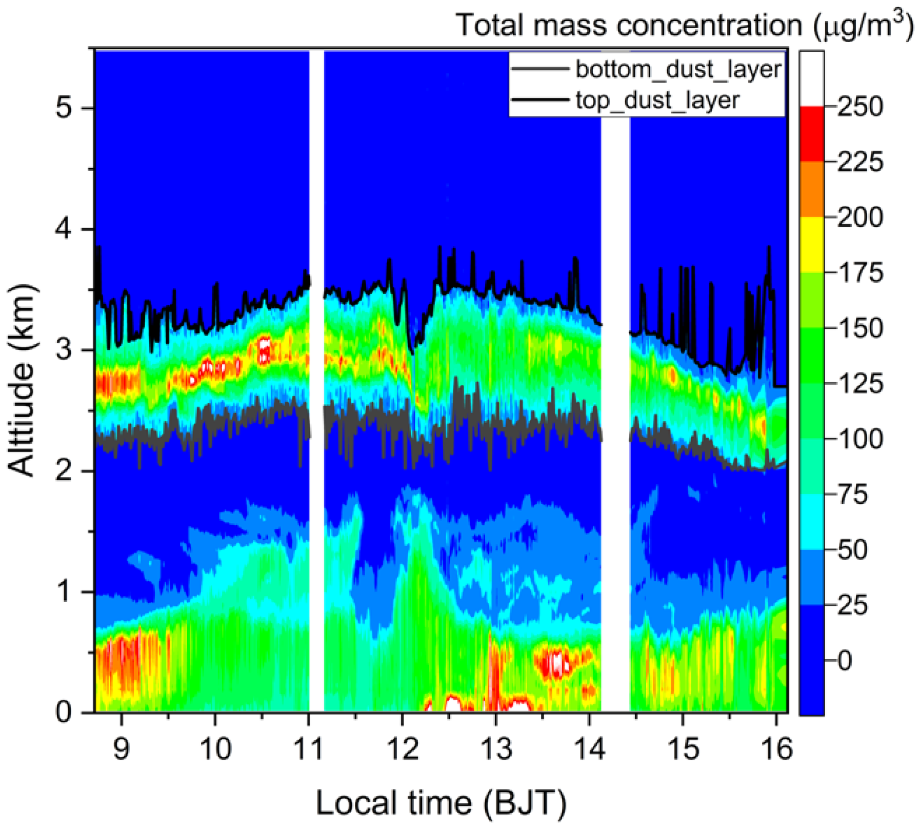
3.2.6. Mass Concentration Profiles

The vertical profiles of the aerosol total mass concentrations derived from the LIDAR measurements using the MEE approach described in Section 2.2 are presented in Figure 9. For this method we used complementary information on the aerosol volume size distributions (VSD), particle density (ρ) and complex refractive index (CRI). The mean columnar VSD derived from the sun photometer measurements showed an almost equal contribution of fine and coarse mode particles all along the mobile transect. For the calculations of the mass concentration, the parameters of the mean VSD were used (

Table 4. Parameters used for the calculations of mass concentration profiles: modal radius for fine ${\mathrm{r}}_{\mathrm{mf}}$ and coarse ${\mathrm{r}}_{\mathrm{mc}}$ modes, in μm; the geometric standard deviation for fine ${\mathsf{\sigma }}_{\mathrm{f}}$ and coarse ${\mathsf{\sigma }}_{\mathrm{c}}$ modes; the ratio of volume concentration of coarse to fine modes ${\mathrm{C}}_{\mathrm{c}}/{\mathrm{C}}_{\mathrm{f}}$; the particle density $\mathsf{\rho }$ in g/cm³; the real part of the refractive index ${\mathrm{m}}_{\mathrm{r}}$; and the imaginary part of the refractive index ${\mathrm{m}}_{\mathrm{i}}$.

	${\mathbf{r}}_{\mathbf{m}\mathbf{f}}$	${\mathbf{r}}_{\mathbf{m}\mathbf{c}}$	${\mathsf{\sigma }}_{\mathbf{f}}$	${\mathsf{\sigma }}_{\mathbf{c}}$	${\mathbf{C}}_{\mathbf{c}}\mathbf{/}{\mathbf{C}}_{\mathbf{f}}$	$\mathsf{\rho }$	${\mathbf{m}}_{\mathbf{r}}$	${\mathbf{m}}_{\mathbf{i}}$
mean	0.13	1.66	0.43	0.68	0.8	1.75	1.5	0.01
std	0.01	0.03	0.01	0.03	0.1	0.34	0.05	0.005
impact on mass (PBL)	7%	0.5%	0.7%	0.6%	4%	20%	13%	1%
impact on mass (dust)	-	2%	-	3%	-	20%	1%	0.1%

).

Using the aerosol properties observed, we defined an urban-industrial aerosol model for the particles inside the PBL, up to 2 km, and a desert dust model for the dust layer at 2.2–3.5 km. The parameters for the urban-industrial aerosol model are summarized in Table 4. As shown is Section 3.2.5, the dust layer in the free troposphere was found to be around 20% of the total AOD from the total column coarse particles. This contribution was subtracted from the total coarse mode VSD and the rest of the VSD was considered as characteristic for the aerosols in the PBL (< 2 km). A bi-modal VSD and a ratio of coarse-to-fine mode particle concentrations (C_c/C_f) of 0.8 was used for the mass calculations below 2 km. The average particle density was calculated based on the chemical composition (sulphate, nitrate, EC, OC, residue) and corresponding particle densities (1.76, 1.73, 2, 1.4, 2.3 g/cm³) following [45], and using the sea salt density (1.3 g/cm³) as in [55]. A value of 1.75 g/cm³ was obtained for the particles inside the PBL. The CRI used for the mass calculations was 1.52–0.008i. For the dust aerosol model, we used a mono-modal coarse mode VSD, a CRI of 1.5–0.005i and a particle density of 2.6 g/cm³, which was characteristic of desert dust [56]. The standard deviations of the parameters in Table 4 correspond to the variability of the retrieved VSD presented in Figure 7d and were propagated to the calculations to show the impact of the different parameters on the mass concentration calculations (Table 4). A MEE of 1.79 m²/g was found for the fine-dominant aerosol model in the PBL and a MEE of 0.54 m²/g was found for the dust layer. Other studies found MEE values of 0.5–1.09 m²/g for Saharan dust [57]. For the fine particles, a higher MEE (2.87–6.64 m²/g) was found for PM_2.5 in cities in China [58], but in our case, the size distribution showed an important contribution of both coarse and fine particles.

Some examples of mass concentration profiles are presented in Figure 10. The mean mass concentration in the desert dust layer was 95 ± 52 μg/m³, with a maximum of 284 μg/m³. The mean mass concentration in the PBL for different segments along the mobile transect is presented in Table 4, and was around 80 ± 62 μg/m³ for the whole transect. The highest particle mass concentrations were recorded near Tianjin city, from 08:30 to 09:30, and when crossing the industrial coastal region, from 12:00 to 14:00.

The PM₁₀ and PM_2.5 fractions of the total particle mass concentrations were calculated as a percentage of the particles with D_p < 10 μm and D_p < 2.5 μm, respectively, from the total volume concentration of the VSD that was defined for aerosols in the PBL. Using this method, it was found that the PM₁₀ and PM_2.5 represented 95% and 56% of the total mass, respectively. The LIDAR-derived PM₁₀ and PM_2.5 mass concentrations at surface level and the hourly PM₁₀ and PM_2.5 recorded at air quality (AQ) stations along the mobile transect are presented in Figure 11. The PM₁₀ and PM_2.5 measured at the AQ stations closest to the mobile transect were considered. No data were available at the AQ stations at 13:00 BJT. Despite all the limits for a direct comparison with AQ measurements and given the uncertainties and assumptions used for the calculations, there is a rather good agreement between the LIDAR-derived aerosol mass concentrations and the AQ measurements.

The calculation of aerosol mass concentration profiles is a complex issue involving numerous assumptions, namely the particles size distribution, particles shape, chemical composition, mixing state and the homogeneity and stationarity of all these parameters with height. Thus, the associated uncertainties are also difficult to evaluate. In this study, the standard deviation of each parameter given in Table 4 was used as a measure of the uncertainty. To this, we added the uncertainty on the extinction profiles, considered to be 25%. The highest uncertainty was introduced by the assumed particle density, with an impact of 20%, followed by the complex refractive index, with an impact of 13% on the mass concentration. Considering the errors as statistically independent, an overall uncertainty of 32% was evaluated for mass concentration profiles. The levels recorded at AQ stations were within the uncertainty of the estimated mass concentrations. In order to give an order of magnitude for the difference between the air quality and the LIDAR-derived mass concentrations, a mean difference was calculated considering the hourly means from the AQ stations and the closest value in time from the LIDAR data. A mean difference of 10% and 42% was obtained for PM₁₀ and PM_2.5, respectively. This comparison was only indicative, since the hourly mean concentrations recorded at the air quality stations were not directly comparable with the 1 min mass concentration values from the mobile measurements. Despite all the assumptions and uncertainties involved in the mass concentration calculations, we believe that the advantages of this method for LIDAR community and for aerosol data modelling outweigh its limitations.

4. Summary and Applications

4.1. Summary

The MOABAI campaign allowed the mapping of the distribution of aerosol pollutants in the Beijing and North China Plain (NCP) region in the spring of 2017, giving access to horizontal and vertical aerosol concentrations. Various atmospheric situations (clean, heavy pollution, dust transport) were observed and analyzed in relation to the synoptic conditions and the vertical aerosol layer height. The highest AOD and lowest PBL heights (0.5–1.5 km) were observed during anticyclonic conditions with low winds originating from the south, while the dust transport up to a 2–3 km altitude was observed when a depression located over Inner Mongolia was pushing strong winds from the direction of the desert, west of the NCP. The lowest AOD were observed when a low-pressure system was located over eastern Inner Mongolia, bringing clean air over Beijing from the north. A comprehensive analysis focused on a case study in a heavily polluted industrial area between the Tianjin and Tangshan cities and the Tianjin port (Binhai New Area), where high extinction coefficients (0.56 km⁻¹) and mass concentrations (~400 μg/m³) were found.

The novelty of this study consisted of deriving the profiles of aerosol mass concentrations from a LIDAR–sun photometer–in situ synergy. Using the columnar volume size distribution retrieved from the spectral AOD sun photometer measurements (using the GRASP algorithm), we evaluated the PM₁₀ and PM_2.5 fractions of the total mass concentrations at ground level. The mass concentration values found in our study compare very well to the air quality measurements at surface level, which validates our method.

4.2. Applications

Numerous studies on air pollution have already been performed in the North China Plain region, although, there are none that have conducted measurements in motion with mobile LIDAR, sun photometer and in situ optical instruments. The novelty of this study consisted of the observations from a mobile vehicle equipped with LIDAR, sun photometer and in situ instruments (nephelometer, aethalometer, particle counter), which was deployed to capture the aerosol spatial distribution in Beijing and the NCP. Constraining the LIDAR inversion with an AOD measured by the sun photometer is much closer to reality than an inversion with an assumed a priori LR for all profiles, which may not be at all relevant for the study of aerosol spatial variability along a transect. Most LIDARs do not see well close to the surface, and therefore miss an important part of the aerosol boundary layer. Photometers measure aerosol properties on the atmospheric column, including the layer never seen, or not accurately seen, by LIDAR close to the surface. In situ data at surface level complement the missing information from the LIDAR in its blind zone. The combination of LIDAR–sun photometer–in situ, which is a good way to profile the entire aerosol column, was presented in this study. In addition, there was a European effort made in the frame of the Aerosol Cloud and Trace Gas Infrastructure (ACTRIS) research infrastructure to put these three distinct communities (LIDAR, sun photometer and in situ instruments) working together, since synergies such as this have been predicted to open the way for new applications in the future. For example, this method is applicable to fixed sites that have in situ, LIDAR and sun photometer instruments. Furthermore, there is a need to develop the use of mobile embedded systems in the frame of atmospheric research infrastructure (RI) and in their operations. These will provide added-value information with respect to fixed systems to extend the observation capacities and associated services. Our work with mobile observation platforms definitely comes under these RI perspective requirements.

The results presented show the potential capabilities of LIDAR measurements for air quality applications, such as spatially mapping the PM₁₀ and PM_2.5 concentrations both at surface level and vertically using a light mobile system with LIDAR. Mass concentration profiles of dust, volcanic ash and smoke plumes and their spatial distribution are key parameters for different authorities. These measurements are valuable for aviation alerts in case of disruptive events (such as volcanic ash intrusions) and tracking aerosol dynamics, and for regional transport, they are useful for air quality modelling. The results of this work demonstrate that a mobile instrumented vehicle would be an excellent tool for the real-time characterization of aerosol variability and pollution levels, both spatially and vertically.

The application domains of such mobile systems having LIDAR and sun photometer instruments are vast. Mapping AOD with a mobile sun photometer allows for the validation of satellite measurements at different scales; no other instrument at ground level can perform that spatially in so many points and in such a short time. Studies showing the profiles of aerosol mass concentration are scarce in the literature. Different aerosol plumes (smoke, dust, volcanic) and their variability can be spatially tracked to the source and their contribution (AOD, mass concentration) to the vertical profile can be evaluated. We have shown the added value of such a mobile system throughout the MOABAI campaign.

As a perspective to further improve the mass concentration profiles, depolarization and spectral elastic backscatter LIDAR measurements can be used to better characterize the aerosol types on the vertical profile. This can be achieved with the dual-wavelength, depolarization micro-pulse CIMEL CE376 LIDAR, which was deployed for the same amount of time and in the same year, 2019, for: (i) mobile on-road measurements of smoke in the Fire Influence on Regional to Global Environments and Air Quality (FIREX-AQ) campaign in the north-western US in the summer of 2019; (ii) for stationary measurements during the Campagne d’Observation Intensive des Aérosols et Précurseurs à Caillouël-Crépigny (COBIACC) campaign in France in the summer of 2019, which focused on the monitoring of background and transported aerosols at a rural site. The mobility of sun–sky photometers is also advancing. On the one side, the CIMEL CE318-T sun–sky–lunar photometer has already been successfully involved in shipborne campaigns [59] and was also deployed during the FIREX-AQ campaign for mobile car measurements. On the other side, the development of an Advanced PLASMA instrument that performs sun and sky measurements is in progress. Recently, in France, the Marion Dufresne ship that is in operation in the Indian Ocean has been equipped with such a CIMEL CE318-T mobile photometer to measure, on a permanent basis, that which AERONET usually measures at a fixed location. In a second step, a LIDAR will also be set up on this mobile exploratory platform. This is opening a new era for joint mobile automatic LIDAR and photometer observations and is really needed to upgrade the Maritime Aerosol Network (MAN), the maritime branch of AERONET, which is still relying on manual measurements. These additional examples show that the number of applications is increasing, to which the ACTRIS European effort will contribute with the development of such platforms and LIDAR–photometer retrievals.

References

1. Chen, H.; Wang, H. Haze days in North China and the associated atmospheric circulations based on daily visibility data from 1960 to 2012. J. Geophys. Res. Atmos. 2015, 120, 5895–5909. [Google Scholar] [CrossRef]
2. Yang, Y.; Wang, H.; Smith, S.J.; Zhang, R.; Lou, S.; Qian, Y.; Ma, P.-L.; Rasch, P.J. Recent intensification of winter haze in China linked to foreign emissions and meteorology. Sci. Rep. 2018, 8, 2107. [Google Scholar] [CrossRef] [PubMed] [Green Version]
3. Han, L.; Zhou, W.; Li, W. Increasing impact of urban fine particles (PM2.5) on areas surrounding Chinese cities. Sci. Rep. 2015, 5, 12467. [Google Scholar] [CrossRef] [PubMed] [Green Version]
4. An, Z.; Huang, R.-J.; Zhang, R.; Tie, X.; Li, G.; Cao, J.; Zhou, W.; Shi, Z.; Han, Y.; Gu, Z.; et al. Severe haze in northern China: A synergy of anthropogenic emissions and atmospheric processes. Proc. Natl. Acad. Sci. USA 2019, 116, 8657–8666. [Google Scholar] [CrossRef] [PubMed] [Green Version]
5. Sun, L.; Li, R.; Tian, X.-P.; Wei, J. Analysis of the temporal and spatial variation of Aerosols in the Beijing-Tianjin-Hebei region with a 1 km AOD product. Aerosol Air Qual. Res. 2017, 17, 923–935. [Google Scholar] [CrossRef] [Green Version]
6. Zhu, Y.; Zhang, J.; Wang, J.; Chen, W.; Han, Y.; Ye, C.; Li, Y.; Liu, J.; Zeng, L.; Wu, Y.; et al. Distribution and sources of air pollutants in the North China Plain based on on-road mobile measurements. Atmos. Chem. Phys. Discuss. 2016, 16, 12551–12565. [Google Scholar] [CrossRef] [Green Version]
7. Lei, Y.; Zhang, Q.; He, K.B.; Streets, D.G. Primary anthropogenic aerosol emission trends for China, 1990–2005. Atmos. Chem. Phys. Discuss. 2011, 11, 931–954. [Google Scholar] [CrossRef] [Green Version]
8. Yu, X.; Lü, R.; Liu, C.; Yuan, L.; Shao, Y.; Zhu, B.; Lei, L. Seasonal variation of columnar aerosol optical properties and radiative forcing over Beijing, China. Atmos. Environ. 2017, 166, 340–350. [Google Scholar] [CrossRef]
9. Li, J. Pollution trends in China from 2000 to 2017: A multi-sensor view from space. Remote. Sens. 2020, 12, 208. [Google Scholar] [CrossRef] [Green Version]
10. Sun, J.; Zhang, M.; Liu, T. Spatial and temporal characteristics of dust storms in China and its surrounding regions, 1960–1999: Relations to source area and climate. J. Geophys. Res. Atmos. 2001, 106, 10325–10333. [Google Scholar] [CrossRef]
11. Ma, Z.; Liu, R.; Liu, Y.; Bi, J. Effects of air pollution control policies on PM2.5 pollution improvement in China from 2005 to 2017: A satellite-based perspective. Atmos. Chem. Phys. Discuss. 2019, 19, 6861–6877. [Google Scholar] [CrossRef] [Green Version]
12. Zhai, S.; Jacob, D.J.; Wang, X.; Shen, L.; Li, K.; Zhang, Y.; Gui, K.; Zhao, T.; Liao, H. Fine particulate matter (PM2.5) trends in China, 2013–2018: Contributions from meteorology. Atmos. Chem. Phys. Discuss. 2019, 19, 11031–11041. [Google Scholar] [CrossRef] [Green Version]
13. Popovici, I.E.; Goloub, P.; Podvin, T.; Blarel, L.; Loisil, R.; Unga, F.; Mortier, A.; Deroo, C.; Victori, S.; Ducos, F.; et al. Description and applications of a mobile system performing on-road aerosol remote sensing and in situ measurements. Atmos. Meas. Tech. 2018, 11, 4671–4691. [Google Scholar] [CrossRef] [Green Version]
14. Freudenthaler, V.; Linné, H.; Chaikovski, A.; Rabus, D.; Groß, S. EARLINET LiDAR quality assurance tools. Atmos. Meas. Tech. Discuss. 2018, 2018, 1–35. [Google Scholar] [CrossRef] [Green Version]
15. Müller, T.; Laborde, M.; Kassell, G.; Wiedensohler, A. Design and performance of a three-wavelength LED-based total scatter and backscatter integrating nephelometer. Atmos. Meas. Tech. 2011, 4, 1291–1303. [Google Scholar] [CrossRef] [Green Version]
16. Drinovec, L.; Močnik, G.; Zotter, P.; Prévôt, A.S.H.; Ruckstuhl, C.; Coz, E.; Rupakheti, M.; Sciare, J.; Müller, T.; Wiedensohler, A.; et al. The “dual-spot” Aethalometer: An improved measurement of aerosol black carbon with real-time loading compensation. Atmos. Meas. Tech. 2015, 8, 1965–1979. [Google Scholar] [CrossRef] [Green Version]
17. Fernald, F.G. Analysis of atmospheric lidar observations: Some comments. Appl. Opt. 1984, 23, 652–653. [Google Scholar] [CrossRef]
18. Klett, J.D. Stable analytical inversion solution for processing lidar returns. Appl. Opt. 1981, 20, 211–220. [Google Scholar] [CrossRef] [PubMed] [Green Version]
19. Mortier, A. Tendances et Variabilites de L’aerosol Atmospherique a L’aide du Couplage Lidar/Photometre sur les Sites de Lille et Dakar. Ph.D. Thesis, University of Lille, Lille, France, 2013. [Google Scholar]
20. Mortier, A.; Goloub, P.; Podvin, T.; Deroo, C.; Chaikovsky, A.; Ajtai, N.; Blarel, L.; Tanre, D.; Derimian, Y. Detection and characterization of volcanic ash plumes over Lille during the Eyjafjallajökull eruption. Atmos. Chem. Phys. Discuss. 2013, 13, 3705–3720. [Google Scholar] [CrossRef] [Green Version]
21. Mortier, A.; Goloub, P.; Derimian, Y.; Tanré, D.; Podvin, T.; Blarel, L.; Deroo, C.; Marticorena, B.; Diallo, A.; Ndiaye, T. Climatology of aerosol properties and clear-sky shortwave radiative effects using Lidar and Sun photometer observations in the Dakar site. J. Geophys. Res. Atmos. 2016, 121, 6489–6510. [Google Scholar] [CrossRef]
22. Popovici, I.E. Aerosol Spatial and Temporal Variability as Seen by Mobile Aerosol Monitoring System (MAMS). 2018. Available online: http://www.theses.fr (accessed on 23 December 2021).
23. Randriamiarisoa, H.; Chazette, P.; Couvert, P.; Sanak, J.; Mégie, G. Relative humidity impact on aerosol parameters in a Paris suburban area. Atmos. Chem. Phys. Discuss. 2006, 6, 1389–1407. [Google Scholar] [CrossRef] [Green Version]
24. Skupin, A.; Ansmann, A.; Engelmann, R.; Seifert, P.; Müller, T. Four-year long-path monitoring of ambient aerosol extinction at a central European urban site: Dependence on relative humidity. Atmos. Chem. Phys. Discuss. 2016, 16, 1863–1876. [Google Scholar] [CrossRef] [Green Version]
25. Pan, X.L.; Yan, P.; Tang, J.; Ma, J.Z.; Wang, Z.F.; Gbaguidi, A.; Sun, Y.L. Observational study of influence of aerosol hygroscopic growth on scattering coefficient over rural area near Beijing mega-city. Atmos. Chem. Phys. Discuss. 2009, 9, 7519–7530. [Google Scholar] [CrossRef] [Green Version]
26. Dubovik, O.; Herman, M.; Holdak, A.; Lapyonok, T.; Tanré, D.; Deuzé, J.L.; Ducos, F.; Sinyuk, A.; Lopatin, A. Statistically optimized inversion algorithm for enhanced retrieval of aerosol properties from spectral multi-angle polarimetric satellite observations. Atmos. Meas. Tech. 2011, 4, 975–1018. [Google Scholar] [CrossRef] [Green Version]
27. Dubovik, O.; Lapyonok, T.; Litvinov, P.; Herman, M.; Fuertes, D.; Ducos, F.; Torres, B.; Derimian, Y.; Huang, X.; Lopatin, A.; et al. GRASP: A versatile algorithm for characterizing the atmosphere. SPIE Newsroom 2014, 2–5. [Google Scholar] [CrossRef]
28. Dubovik, O.; Li, Z.; Mishchenko, M.I.; Tanré, D.; Karol, Y.; Bojkov, B.; Cairns, B.; Diner, D.J.; Espinosa, W.R.; Goloub, P.; et al. Polarimetric remote sensing of atmospheric aerosols: Instruments, methodologies, results, and perspectives. J. Quant. Spectrosc. Radiat. Transf. 2019, 224, 474–511. [Google Scholar] [CrossRef]
29. Torres, B.; Dubovik, O.; Fuertes, D.; Schuster, G.; Cachorro, V.E.; Lapyonok, T.; Goloub, P.; Blarel, L.; Barreto, A.; Mallet, M.; et al. Advanced characterisation of aerosol size properties from measurements of spectral optical depth using the GRASP algorithm. Atmos. Meas. Tech. 2017, 10, 3743–3781. [Google Scholar] [CrossRef] [Green Version]
30. Torres, B.; Fuertes, D. Characterization of aerosol size properties from measurements of spectral optical depth: A global validation of the GRASP-AOD code using long-term AERONET data. Atmos. Meas. Tech. 2021, 14, 4471–4506. [Google Scholar] [CrossRef]
31. Lagrosas, N.; Kuze, H.; Takeuchi, N.; Fukagawa, S.; Bagtasa, G.; Yoshii, Y.; Naito, S.; Yabuki, M. Correlation study between suspended particulate matter and portable automated lidar data. J. Aerosol Sci. 2005, 36, 439–454. [Google Scholar] [CrossRef]
32. Lewandowski, P.A.; Eichinger, W.E.; Holder, H.; Prueger, J.; Wang, J.; Kleinman, L.I. Vertical distribution of aerosols in the vicinity of Mexico City during MILAGRO-2006 Campaign. Atmos. Chem. Phys. Discuss. 2010, 10, 1017–1030. [Google Scholar] [CrossRef] [Green Version]
33. Stein, A.F.; Draxler, R.R.; Rolph, G.D.; Stunder, B.J.B.; Cohen, M.D.; Ngan, F. NOAA’s HYSPLIT atmospheric transport and dispersion modeling system. Bull. Am. Meteorol. Soc. 2015, 96, 2059–2077. [Google Scholar] [CrossRef]
34. Li, W.; Wang, W.; Zhou, Y.; Ma, Y.; Zhang, D.; Sheng, L. Occurrence and reverse transport of severe dust storms associated with synoptic weather in East Asia. Atmosphere 2018, 10, 4. [Google Scholar] [CrossRef] [Green Version]
35. Kong, S.; Han, B.; Bai, Z.; Chen, L.; Shi, J.; Xu, Z. Receptor modeling of PM2.5, PM10 and TSP in different seasons and long-range transport analysis at a coastal site of Tianjin, China. Sci. Total. Environ. 2010, 408, 4681–4694. [Google Scholar] [CrossRef]
36. Su, X.; Wang, Q.; Li, Z.; Calvello, M.; Esposito, F.; Pavese, G.; Lin, M.; Cao, J.; Zhou, C.; Li, N.; et al. Regional transport of anthropogenic pollution and dust aerosols in spring to Tianjin—A coastal megacity in China. Sci. Total. Environ. 2017, 584–585, 381–392. [Google Scholar] [CrossRef]
37. Ni, T.; Li, P.; Han, B.; Bai, Z.; Ding, X.; Wang, Q.; Huo, J.; Lu, B. Spatial and temporal variation of chemical composition and mass closure of ambient PM10 in Tianjin, China. Aerosol Air Qual. Res. 2013, 13, 1832–1846. [Google Scholar] [CrossRef] [Green Version]
38. Lyu, L.; Dong, Y.; Zhang, T.; Liu, C.; Liu, W.; Xie, Z.; Xiang, Y.; Zhang, Y.; Chen, Z.; Fan, G.; et al. Vertical distribution characteristics of PM2.5 observed by a mobile vehicle lidar in Tianjin, China in 2016. J. Meteorol. Res. 2018, 32, 60–68. [Google Scholar] [CrossRef]
39. Hildemann, L.M.; Markowski, G.R.; Jones, M.C.; Cass, G.R. Submicrometer Aerosol mass distributions of emissions from boilers, fireplaces, automobiles, diesel trucks, and meat-cooking operations. Aerosol Sci. Technol. 1991, 14, 138–152. [Google Scholar] [CrossRef]
40. Merico, E.; Donateo, A.; Gambaro, A.; Cesari, D.; Gregoris, E.; Barbaro, E.; Dinoi, A.; Giovanelli, G.; Masieri, S.; Contini, D. Influence of in-port ships emissions to gaseous atmospheric pollutants and to particulate matter of different sizes in a Mediterranean harbour in Italy. Atmos. Environ. 2016, 139, 1–10. [Google Scholar] [CrossRef]
41. Petzold, A.; Hasselbach, J.; Lauer, P.; Baumann, R.; Franke, K.; Gurk, C.; Schlager, H.; Weingartner, E. Experimental studies on particle emissions from cruising ship, their characteristic properties, transformation and atmospheric lifetime in the marine boundary layer. Atmos. Chem. Phys. Discuss. 2008, 8, 2387–2403. [Google Scholar] [CrossRef] [Green Version]
42. Popovicheva, O.; Kireeva, E.; Shonija, N.; Zubareva, N.; Persiantseva, N.; Tishkova, V.; Demirdjian, B.; Moldanová, J.; Mogilnikov, V. Ship particulate pollutants: Characterization in terms of environmental implication. J. Environ. Monit. 2009, 11, 2077–2086. [Google Scholar] [CrossRef] [PubMed]
43. Randles, C. Hygroscopic and optical properties of organic sea salt aerosol and consequences for climate forcing. Geophys. Res. Lett. 2004, 31, 4–7. [Google Scholar] [CrossRef]
44. Liu, X.; Cheng, Y.; Zhang, Y.; Jung, J.; Sugimoto, N.; Chang, S.-Y.; Kim, Y.J.; Fan, S.; Zeng, L. Influences of relative humidity and particle chemical composition on aerosol scattering properties during the 2006 PRD campaign. Atmos. Environ. 2008, 42, 1525–1536. [Google Scholar] [CrossRef]
45. Han, S.; Bian, H.; Zhang, Y.; Wu, J.; Wang, Y.; Tie, X.; Li, Y.; Li, X.; Yao, Q. Effect of Aerosols on visibility and radiation in Spring 2009 in Tianjin, China. Aerosol Air Qual. Res. 2012, 12, 211–217. [Google Scholar] [CrossRef] [Green Version]
46. Schuster, G.L.; Lin, B.; Dubovik, O. Remote sensing of aerosol water uptake. Geophys. Res. Lett. 2009, 36, 1–5. [Google Scholar] [CrossRef]
47. Cattrall, C.; Reagan, J.; Thome, K.; Dubovik, O. Variability of aerosol and spectral lidar and backscatter and extinction ratios of key aerosol types derived from selected Aerosol Robotic Network locations. J. Geophys. Res. Space Phys. 2005, 110, 1–13. [Google Scholar] [CrossRef]
48. Müller, D.; Ansmann, A.; Mattis, I.; Tesche, M.; Wandinger, U.; Althausen, D.; Pisani, G. Aerosol-type-dependent lidar ratios observed with Raman lidar. J. Geophys. Res. Space Phys. 2007, 112, 16202. [Google Scholar] [CrossRef]
49. Ackermann, J. The extinction-to-backscatter ratio of tropospheric Aerosol: A numerical study. J. Atmos. Ocean. Technol. 1998, 15, 1043–1050. [Google Scholar] [CrossRef]
50. Müller, D.; Franke, K.; Wagner, F.; Althausen, D.; Ansmann, A.; Heintzenberg, J. Vertical profiling of optical and physical particle properties over the tropical Indian Ocean with six-wavelength lidar: 1. Seasonal cycle. J. Geophys. Res. Earth Surf. 2001, 106, 28567–28575. [Google Scholar] [CrossRef]
51. Hänel, A.; Baars, H.; Althausen, D.; Ansmann, A.; Engelmann, R.; Sun, J.Y. One-year aerosol profiling with EUCAARI Raman lidar at Shangdianzi GAW station: Beijing plume and seasonal variations. J. Geophys. Res. Space Phys. 2012, 117, 1–11. [Google Scholar] [CrossRef] [Green Version]
52. Boyouk, N.; Léon, J.-F.; Delbarre, H.; Augustin, P.; Fourmentin, M. Impact of sea breeze on vertical structure of aerosol optical properties in Dunkerque, France. Atmos. Res. 2011, 101, 902–910. [Google Scholar] [CrossRef]
53. Ansmann, A.; Althausen, D.; Wandinger, U.; Wagner, F.; Mueller, D.; Herber, A. European pollution outbreaks during ACE 2: Lofted aerosol plumes observed with Raman lidar at the Portuguese coast. J. Geophys. Res. Earth Surf. 2001, 106, 20725–20733. [Google Scholar] [CrossRef]
54. Wang, H.; Xu, X.; Zhu, G. Landscape changes and a salt production sustainable approach in the State of Salt pan area decreasing on the coast of Tianjin, China. Sustainability 2015, 7, 10078–10097. [Google Scholar] [CrossRef]
55. Tsekeri, A.; Lopatin, A.; Amiridis, V.; Marinou, E.; Igloffstein, J.; Siomos, N.; Solomos, S.; Kokkalis, P.; Engelmann, R.; Baars, H.; et al. GARRLiC and LIRIC: Strengths and limitations for the characterization of dust and marine particles along with their mixtures. Atmos. Meas. Tech. 2017, 10, 4995–5016. [Google Scholar] [CrossRef] [Green Version]
56. Reid, J.S.; Jonsson, H.H.; Maring, H.B.; Smirnov, A.; Savoie, D.L.; Cliff, S.S.; Reid, E.A.; Livingston, J.M.; Meier, M.M.; Dubovik, O.; et al. Comparison of size and morphological measurements of coarse mode dust particles from Africa. J. Geophys. Res. Atoms. 2003, 108, 8593. [Google Scholar] [CrossRef] [Green Version]
57. Córdoba-Jabonero, C.; Andrey-Andrés, J.; Gomez, L.; Adame, J.A.; Sorribas, M.; Navarro-Comas, M.; Puentedura, O.; Cuevas, E.; Gil-Ojeda, M. Vertical mass impact and features of Saharan dust intrusions derived from ground-based remote sensing in synergy with airborne in-situ measurements. Atmos. Environ. 2016, 142, 420–429. [Google Scholar] [CrossRef]
58. Cheng, Z.; Ma, X.; He, Y.; Jiang, J.; Wang, X.; Wang, Y.; Sheng, L.; Hu, J.; Yan, N. Mass extinction efficiency and extinction hygroscopicity of ambient PM2.5 in urban China. Environ. Res. 2017, 156, 239–246. [Google Scholar] [CrossRef] [PubMed]
59. Yin, Z.; Ansmann, A.; Baars, H.; Seifert, P.; Engelmann, R.; Radenz, M.; Jimenez, C.; Herzog, A.; Ohneiser, K.; Hanbuch, K.; et al. Aerosol measurements with a shipborne Sun–sky–lunar photometer and collocated multiwavelength Raman polarization lidar over the Atlantic Ocean. Atmos. Meas. Tech. 2019, 12, 5685–5698. [Google Scholar] [CrossRef] [Green Version]
Figure 1. (a) Area investigated by the mobile measurements during the MOABAI campaign (blue) and the North China Plain (red), (b) GPS track of all mobile transects and (c) IAP instrumented van used for the mobile observations.
Atmosphere 13 00021 g001
Figure 2. Spatial variability of AOD at 440 nm (top panels (af)) and Angstrom Exponent (AE) between 440 and 870 nm (bottom panels (gl)), derived from PLASMA sun photometer measurements. The A, B and C (d,k) denote the departure and end points for the three transects: Beijing–Tianjin (AB) on 16 May 2017, Tianjin–Tangshan (BC) on 17 May 2017 and Tangshan–Beijing (CA) on 18 May 2017. Please note that the color scale for the AOD maps is different for each transect in order to show the fine spatial variability.
Atmosphere 13 00021 g002
Figure 3. (Top panels (ag)) Spatio-temporal and vertical variability of aerosol layers and clouds, color-coded by LIDAR Range Corrected Signal (RCS) as measured along the mobile transects detailed in Table 2 and depicted in Figure 2; (Middle panels (hn)) AOD at 440 nm; (Bottom panels (ou)) PBL heights from mobile LIDAR measurements.
Atmosphere 13 00021 g003
Figure 4. (a) GPS track of the mobile measurements from Tianjin to Tangshan, color-coded by 30 min time intervals (local time, UTC +8 h) and (b) particle volume size distributions measured by Grimm Sky-OPC, averaged on 30 min transect segments.
Atmosphere 13 00021 g004
Figure 5. Spatio-temporal variability of: (a) particle volume size distribution as measured by Grimm Sky-OPC; (b) scattering coefficient measured by nephelometer (black), scattering coefficient corrected for RH effect (green), absorption coefficient derived from aethalometer (cyan) and extinction coefficient computed from nephelometer and aethalometer measurements (magenta); and (c) T (black) and RH (blue) measured by the weather station along the mobile transect from Tianjin to Tangshan on 17 May 2017.
Atmosphere 13 00021 g005
Figure 6. Spatio-temporal variability of aerosol extinction coefficients at 525 nm derived from in situ measurements (nephelometer and aethalometer) with no correction for RH (black) and with f(RH) correction (magenta), and LIDAR-derived extinction coefficients at 532 nm at a 210 m altitude (green). The green shaded area represents the uncertainty on the derived extinction coefficients.
Atmosphere 13 00021 g006
Figure 7. Spatio-temporal variability of (a) Angstrom Exponent (AE), (b) spectral AOD, (c) total column VSD retrieved with GRASP-AOD for every transect segment and (d) columnar VSD for some time intervals along the mobile transect. All size distributions were averaged on 30 min time intervals and can be localized on the mobile transect using the map color-coded by local time in Figure 4a.
Atmosphere 13 00021 g007
Figure 8. (a) 3D plot of the LIDAR-derived extinction profiles at 532 nm along the mobile transect from Tianjin to Tangshan and (b) 72 h backward trajectories arriving at a point along the mobile transect, near the Tianjin port (38.82° N, 117.59° E) on 17 May 2017, 05:00 UTC, at heights of 0 m (red), 500 m (blue) and 3000 m (green).
Atmosphere 13 00021 g008
Figure 9. Aerosol total mass concentration profiles derived using the MEE approach on 17 May 2017 along the transect from Tianjin to Tangshan (BJT = Beijing time). The calculations were done considering a dust aerosol model for the layer in the 2–3.5 km range and an urban-industrial aerosol model for the rest of the profile.
Atmosphere 13 00021 g009
Figure 10. (Left) Aerosol extinction coefficient profiles and LR at 532 nm and (right) mass concentrations profiles for different times along the mobile transect: 08:55 (a,b); 10:50 (c,d); 12:30 (e,f); 13:00 (g,h); and 15:20 (i,j), local time. The extinction profiles were derived using the in situ constraint corrected for the RH.
Atmosphere 13 00021 g010
Figure 11. Spatio-temporal variability of (a) PM10 (green) and (b) PM2.5 (red) at surface level, derived from LIDAR profiles, and the mean hourly PM10 (magenta) and PM2.5 (cyan), measured at the closest air quality (AQ) stations to the route (BJT = Beijing time). The shaded area on each curve represents the uncertainty of 32% on the LIDAR-derived mass concentrations.
Atmosphere 13 00021 g011