Abstract
Future climate change is expected to impact the natural systems. This study used future climate data of general circulation models (GCMs) to investigate the impacts of climate change during the future period (2062–2095) relative to the historical period (1981–2014) on the hydrological system of the Minjiang river watershed, China. A previously calibrated soil and water assessment tool (SWAT) was employed to simulate the future hydrology under the impacts of changes in temperature, precipitation, and atmospheric CO2 concentration for four shared socioeconomic pathways (SSP 1, 2, 3, and 5) of the CMIP6. The study revealed that the impacts of increase in future temperature, i.e., increase in ET, and decrease in surface runoff, water, and sediment yield will be countered by increased atmospheric [CO2], and changes in the hydrological parameters in the future will be mostly associated to changes in precipitation. Data of the GCMs for all the SSPs predicts increase in precipitation of the watershed, which will cause increase in surface runoff, water yield, and sediment yield. Surface runoff will increase more in SSP 5 (47%), while sediment and water yield will increase more in SSP 1, by 33% and 23%, respectively. At the seasonal scale, water yield and surface runoff will increase more in autumn and winter in SSP 1, while in other scenarios, these parameters will increase more in the spring and summer seasons. Sediment yield will increase more in autumn in all scenarios. Similarly, the future climate change is predicted to impact the important parameters related to the flow regime of the Minjiang river, i.e., the frequency and peak of large floods (flows > 14,000 m3/s) will increase along the gradient of scenarios, i.e., more in SSP 5 followed by 3, 2, and 1, while duration will increase in SSP 5 and decrease in the other SSPs. The frequency and duration of extreme low flows will increase in SSP 5 while decrease in SSP 1. Moreover, peak of extreme low flows will decrease in all scenarios except SSP 1, in which it will increase. The study will improve the general understanding about the possible impacts of future climate change in the region and provide support for improving the management and protection of the watershed’s water and soil resources.
1. Introduction
According to the intergovernmental panel on climate change (IPCC) [1], global atmospheric concentrations of greenhouse gases, i.e., carbon dioxide (CO2), methane, and nitrous oxide, have increased substantially due to economic and population growth. The effect of increasing greenhouse gases is detected throughout the climate system and is the dominant cause of the observed warming since the middle of the 20th century. Limiting climate change would mainly require reductions in greenhouse gas emissions which, together with adaptation, can limit climate change risks [1]. With the increased awareness of the impacts of greenhouse gas emissions on the global climatic system, the policy world under the Paris agreement has embraced the limiting of greenhouse gas emissions by gradually adopting alternative socioeconomic and development strategies. The dependance of the global climate system on greenhouse gas emissions and socioeconomic and development strategies makes the future climate and its impacts on the natural systems uncertain. Shared socioeconomic pathways (SSPs) based on alternative socioeconomic development policies are constructed to facilitate the future climate change and impact studies, i.e., SSP 1 leads gradually toward a sustainable and green development, SSP 5 leads toward the continuation of fossil fuel development, whereas SSP 2, 3, and 4 are intermediate scenarios [2].
General Circulation Models (GCMs) developed in the Coupled model intercomparison project (CMIP) of the world climate research programme (WCRP) are the tools for understanding the mechanisms of past climate and projecting possible future climate change under idealized emission assumptions. GCMs generate meteorological variables such as precipitation, temperature, solar radiation, wind speed, relative humidity, etc., for different climate change scenarios, by solving the primitive equations of thermodynamics, mass, and momentum [3]. However, numerous studies have reported that climate simulations of the GCMs contain biases and uncertainties [4,5]. Uncertainty in process representation and error propagation, as well as in specified greenhouse gases, aerosol emissions, land use change, and sensitivity to resolution, affect model results. These biases vary from one model to another for certain variables, but no individual model clearly emerged as ‘the best’ overall [6]. Hence, their direct use as inputs for impact models is inadvisable since they might lead to inaccurate conclusions. Therefore, to use climate data from GCMs for impact assessment, bias correction is a prerequisite step. Bias correction is the adjustment of biased simulated data to observations. Several bias correction methods have been developed ranging from simple scaling approaches to distribution mapping [7].
Apart from the role in climate change as a greenhouse gas, elevated atmospheric CO2 concentration decreases stomatal conductance, thus reduces the leaf loss of water [8,9]. Therefore, increased atmospheric CO2 concentration together with climate change are expected to alter hydrological systems worldwide. The most widely used method for the impact assessment of climate change on hydrological processes involve forcing watershed-scale hydrological models such as the soil and water assessment tool (SWAT) with the outputs of GCMs. The SWAT model is a watershed-scale, physically based, continuous-time hydrologic and water quality model [10]. Recently several studies have employed the SWAT model to estimate the impacts of future climate change on watershed systems worldwide. For example, the authors of [11] evaluated the impacts of future climate change using the SWAT model in the Jhelum river basin and found a general increase in streamflow. The authors of [12] simulated the impacts of future climate change on the hydrology of the Krishna river basin and found an increase in surface runoff, streamflow, and water yield. The authors of [13] simulated the impacts of future climate change in the Ndembera river watershed and found that the warmer future climate will increase evapotranspiration and decrease water yield.
The Minjiang river watershed is a humid, subtropical, forest-dominated and one of the largest watersheds in China. It is an ecologically and economically important, abundant water resource. It plays a great role in socio-economic development and provides opportunities for hydroelectricity generation, navigation, irrigation, fishing, recreation, and biodiversity conservation [14]. Therefore, it is very important to evaluate the impacts of future climate change on the hydrological system of the watershed to support the management and climate change adaptation strategies. The objective of this study is to evaluate the impacts of future precipitation, temperature, and atmospheric [CO2] individually and combinedly on different hydrological components of the Minjiang river watershed for multiple SSP scenarios. The study will improve the general understanding about the possible impacts of future climate change in the region and provide support for improving the management and protection of the watershed’s water and soil resources in this context.
2. Methodology
2.1. Minjiang River Watershed
The Minjiang River watershed is located between 116°30′ and 119°30′ E and 25°20′ and 28°25′ N in the Fujian province of China (Figure 1). It is the largest watershed in the province, covering an area of about 60,900 km2. Its elevation ranges from 0 to 2158 m. The main channel of the Minjiang river flows through Nanping, Fuzhou into the Taiwan strait. Tributary channels flow through Shunchang, Sanming, Jianou, Youxi, Gutian, and Yongtai counties. The Minjiang river watershed is situated in a humid subtropical climate, influenced by the east Asia monsoon. Temperature ranges from 5 to 10 °C in January and from 25 to 30 °C in July. The soil type of the watershed is mainly red soil, and the terrain is hilly and steep, prone to soil erosion and landslides. More than 50% of the land is covered by coniferous forests; other dominant landcover classes are evergreen broad-leaved forest, mixed coniferous and broad-leaved forests, shrub/grasslands, croplands, wetlands, and urban land.
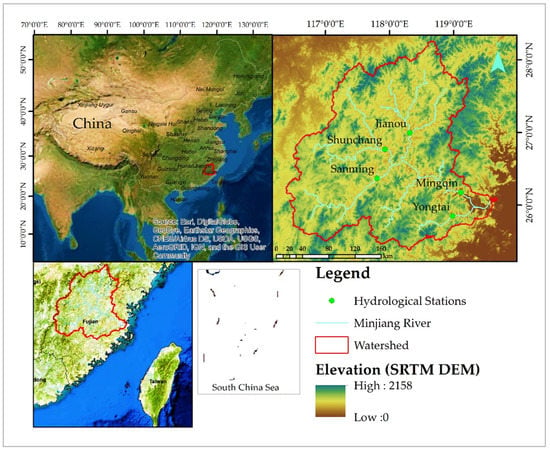
Figure 1.
Location of the Minjiang river, its main tributaries, watershed, and hydrological stations.
2.2. SWAT Model Setup and Calibration
In this study, we used a previously calibrated SWAT model. A detailed description about the setup, calibration, and performance of the model in the Minjiang river watershed can be found in our previous article [15]. Here, we give a brief introduction of the input data, the calibration strategy, and performance of the model.
The SWAT model is GIS based with interfaces for ArcGIS and QGIS. Structurally, the model divides a watershed into sub basins; the input values for each sub basin are grouped into climate, Hydrologic response units (HRUs), main channel, and ponds/reservoirs. The HRUs are lumped land units which are the product of a distinct combination of land use, slope, and soil type within the sub basin. To set up the model for the Minjiang river watershed, input data from multiple sources were used, i.e., a digital elevation model (DEM) from the shuttle radar topography mission (SRTM) with a resolution of 30 m, daily scale meteorological data from “The China meteorological assimilation driving datasets for SWAT” (CMADS L V 1.0), for the period 1979–2018 [16,17,18], a soil map from the harmonized world soil database (HWSD) from the food and agriculture organization (FAO) [19], four landcover maps from the European space agency climate change initiative (CCI-LC) [20], and ponds/reservoirs identified using digital maps and images. ArcSWAT version 2012 was used for the model setup, which delineated the watershed into 35 subbasins and 4100 HRUs. The SWAT land use tool (SWAT-LUT) [21] was used for dynamic updating of landcover on a yearly basis.
For the model calibration and performance evaluation, we used monthly observed streamflow data of one location (Mingqin), and yearly data of four locations (Yontai, Shunchang, Sanming, and Jianou) (Figure 1). Moreover, yearly sediment loading data of the above-mentioned five stations within the watershed were used to assess the model performance in terms of simulating the soil erosion and sediment transport. The observed stream flow and sediment loading data were provided by the Fujian department of water resources. The calibration and validation period was 1989–2018 with a warmup period of ten years (1979–1988). Sequential uncertainty fitting (SUFI-2) in SWAT-CUP software [22] was used for sensitivity analysis and calibration of the model. Two objective functions were used for evaluating the performance, i.e., the Coefficient of determination (R2) and the Nash–Sutcliffe efficiency [23]. Overall, the performance of the model was within the acceptable range according to the statistical criteria described in previous studies, i.e., the R2 and NSE values for streamflow ranged from 0.8 to 0.9 and from 0.7 to 0.9, respectively, and for sediment loadings, the R2 and NSE values ranged from 0.6 to 0.8 and from 0.6 to 0.7 during calibration and from 0.7 to 0.9 and 0.7 to 0.9 during validation, respectively. The performance was higher when simulating streamflow than sediment loadings, which was largely influenced by the reservoirs. The calibrated parameters’ descriptions and fitted values for the five locations within the watershed are given in Table 1. More detailed discussion about the model performance can be found in our previous study [15].

Table 1.
Calibrated parameter descriptions and fitted values.
2.3. Evaluating the Impacts of Future Climate Change
To evaluate the impacts of future climate change on the hydrological components of the watershed, this study was divided into three steps. The steps are given in the workflow diagram (Figure 2) and described below:
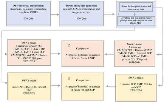
Figure 2.
Workflow diagram of the evaluation of the impacts of future climate change.
In step 1, we downscaled and bias corrected the historical temperature and precipitation data of ten GCMs from CMIP6 [24] (Table 2), and evaluated their agreement to the reference datasets, i.e., CMADS’ temperature and precipitation monthly time series (1979–2014) using Pearson correlation. All of the GCM data were downloaded from the website; https://cds.climate.copernicus.eu (accessed on 22 September 2021). We selected the temperature data of one GCM with the bias correction method that showed the highest agreement with the reference data. Due to the importance of precipitation in the watershed and the reported uncertainties, we selected precipitation data from four GCMs with the bias correction methods, which showed the highest agreement to the reference time series (CMADS) for use in the further steps.

Table 2.
List of GCMs evaluated in the study.
In step 2, we used the selected precipitation and the selected temperature data of GCMs, and different atmospheric CO2 concentrations (350, 550, 700, and 800 ppm), for four shared socioeconomic pathways’ SSPs, i.e., 1, 2, 3, and 5 (Table 3) separately in the SWAT model for the future period (2062–2095) to evaluate their individual impacts. We used the 2nd half of the 21st century to evaluate the impacts on hydrology because the uncertainty among different SSPs would be maximal in that period.

Table 3.
SSP scenarios considered in the study.
In step 3, we used the precipitation along with temperature data of the selected GCMs, and different CO2 concentrations (350, 550, 700, and 800 ppm), for four SSPs together in the SWAT model to evaluate the combined impacts on the hydrology of the watershed. The historical period was 1981–2014, while the future period was 1962–2095. A warmup period of two years was considered during the simulation of both the intervals.
2.4. Downscaling and Bias Correction
We used the CMhyd tool [35] for downscaling and bias correction. Three bias correction methods were used for temperature and precipitation data individually, i.e., distribution mapping (DM) and linear scaling (LS) for both temperature and precipitation, and power transformation (PT) for precipitation and variance scaling (VS) for temperature only. All these methods correct the data on a monthly scale. Detailed descriptions of the equations used by the CMhyd tool are given in [7].
2.5. Hydrological Parameters
2.5.1. Basin Parameters
We evaluated the impacts of future climate change on four hydrological parameters simulated by the SWAT model, i.e., evapotranspiration (ET mm), water yield mm, surface runoff mm, and sediment yield t/ha. ET is the loss of water to the atmosphere. Three different methods for the estimation of ET are available in the SWAT model. We selected the Penman–Monteith method, which is widely used, because it considers the effect of atmospheric CO2 concentration. The SWAT model simulates the effects of atmospheric CO2 concentration on plant canopy resistance and radiation use efficiency. Generally, a doubling of CO2 concentration leads to a general decrease of 40% in stomatal conductance [36]. Water yield is the water leaving the watershed in the form of surface, lateral, and groundwater flow. Surface runoff or overland flow is the water flowing over soil, vegetation, or other ground cover instead of infiltrating. The SWAT model uses the SCS curve number method for surface runoff estimation. Sediment yield refers to the amount of sediment exported along with flowing water by a watershed over a period. The SWAT model uses the Modified Universal Soil Loss Equation (MUSLE) for the estimation of soil erosion. A detailed description of the methods and equations used by the SWAT model is given in the SWAT theoretical documentation [37].
2.5.2. River Flow
We used the indicators of hydrologic alteration (IHA) tool for estimation of the extreme low flows (peak, duration, and frequency), minimum/maximum flow peaks (1, 3, 7, 30, and 90 days), and small/large floods (peak, duration and frequency) at the watershed outlet. All the parameters were the mean values of that period. The IHA tool allows calculation of the floods and extreme low flows parameters using three different methods, i.e., year return interval, percent of daily flows, and cubic meters per second (m3/s). We selected the third option, m3/s, because our study period was divided into two intervals and separate analysis was carried out for each period. Therefore, in order to make a comparison between the two separate intervals, uniform threshold values were set for the analysis. Thresholds for different flow parameters were set according to the data extremes, i.e., extreme low flows were less than 500 m3/s, small floods were higher than 9000 m3/s, and large floods were flows greater than 14,000 m3/s.
3. Results
3.1. GCM Data and Bias Correction Performance
3.1.1. Temperature
Temperature data of the GCMs showed a great agreement with the reference time series. All the bias correction methods improved the agreement. The correlation was higher than 0.95 for all the GCMs after bias correction (Table 4). The marginal plot between the reference and EC-Earth average temperature monthly time series (1979–2014) shows a tight relationship and almost similar distribution of the data points (Figure 3). We randomly selected EC-Earth with variance scaling for use in further sections of the study.

Table 4.
Correlations between temperature reference data and GCMs data with different bias correction methods.
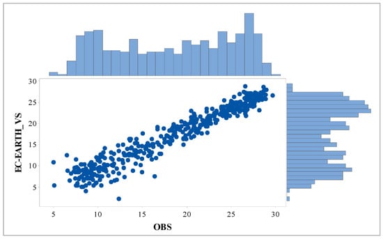
Figure 3.
Marginal plot between reference temperature monthly time series (OBS) and EC-Earth with variance scaling.
3.1.2. Precipitation
Precipitation data from all the GCMs showed large uncertainties. The performance of bias correction was different among the GCMs and methods (Table 5). Overall, the raw data of EC-Earth showed the highest agreement with the reference time series; however, the similarity was still not enough to simulate the actual future hydrology with minimum uncertainties (Figure 4). However, we can use the GCM data and extract the variation between the historical and future hydrological data. This way, we can conclude that the variation that is present is caused by the influencing factors included in the GCM, i.e., rising greenhouse gases, etc. This method is commonly used in impact studies, and is known as delta change correction. However, in delta change correction, delta is extracted on a monthly scale, and thus, the daily scale variations simulated by GCM are ignored. To minimize uncertainties among different GCMs, we used an ensemble mean of multiple GCMs, i.e., Fgoals and BCC-CMS with power transformation, MRI with linear scaling, and raw data of EC-Earth. The BCC-CMS data for SSP 1 was not available; therefore, data from three GCMs was used for this SSP.

Table 5.
Correlations between precipitation reference data and GCMs data with different bias correction methods.
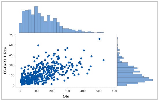
Figure 4.
Marginal plot between reference precipitation monthly time series (OBS) and raw EC-Earth data.
3.2. Impacts of Future Climate Change and Atmospheric [CO2]
3.2.1. Individual Impacts of Future Precipitation, Temperature, and atmospheric [CO2]
Increase in precipitation across the SSPs, with more increase in SSP 1 followed by 2, 5 and 3, will increase the surface runoff, water yield, and sediment yield. Increase in temperature and [CO2] will have smaller impacts than precipitation on the hydrological parameters, with the exception of ET. The impacts of temperature and [CO2] will be opposite to each other, i.e., an increase in temperature will increase ET, while increase in [CO2] will decrease it. Similarly, an increase in temperature will decrease surface runoff, water yield, and sediment yield, while increase in [CO2] will increase surface runoff, water yield, and sediment yield. Thus, the impacts of temperature will be countered by increase in [CO2], with the exception of sediment yield, because the magnitude of the decrease in sediment yield in response to temperature will be more than its increase in response to [CO2] (Figure 5).
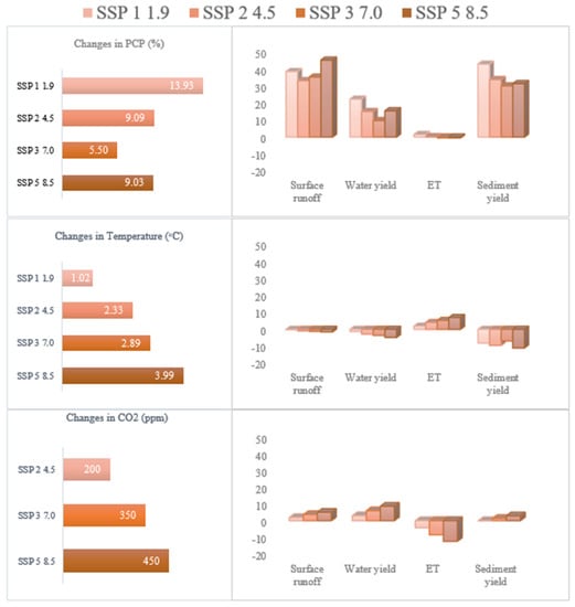
Figure 5.
Changes in precipitation, temperature, and atmospheric [CO2] for different SSPs (left) and their individual impacts on the hydrological parameters (% change) (right).
3.2.2. Combined Impacts of Future Precipitation, Temperature, and Atmospheric [CO2]
Basin Parameters
Surface runoff will be the most influenced hydrological parameter in the watershed. In the case of SSP 5, the annual surface runoff will increase by 48%, while in the case of the other SSPs it will increase by 33–40%. Sediment yield will be the second most influenced parameter. In the case of SSP 1, the annual sediment yield will increase by 33%, while in the case of the other SSPs, it will increase by 20–25%. The annual average water yield will increase by 23% in the case of SSP 1, while it will increase by 10–17% in the remaining SSPs. The ET will decrease by 5% and 3% in the case of SSP 5 and 3, respectively, while it will slightly increase in SSP 1 and 2 (Figure 6).
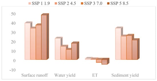
Figure 6.
Combined impacts of precipitation, temperature, and atmospheric [CO2] at an annual scale (% change).
Seasonally, spring surface runoff will increase by 30–42% with little difference among SSPs. In summer, it will increase by 70% in the case of SSP 5, while in the other SSPs, it will increase by 40–50%. In autumn and winter, surface runoff will increase more, by 88% and 46%, respectively, in the case of SSP 1. Water yield will follow the pattern of surface runoff, i.e., in summer, it will increase more in the case of SSP 5, while in autumn and winter, it will increase more in the case of SSP 1. ET will increase in all the seasons in the case of SSP 1, while in the case of SSP 5, it will increase only in autumn. In the other SSPs, ET will experience comparatively smaller impacts across the seasons. In summer and autumn, sediment yield will increase more in the case of SSP 5 and 3, while in winter and spring, it will increase more in SSP 1 and 2 (Figure 7).
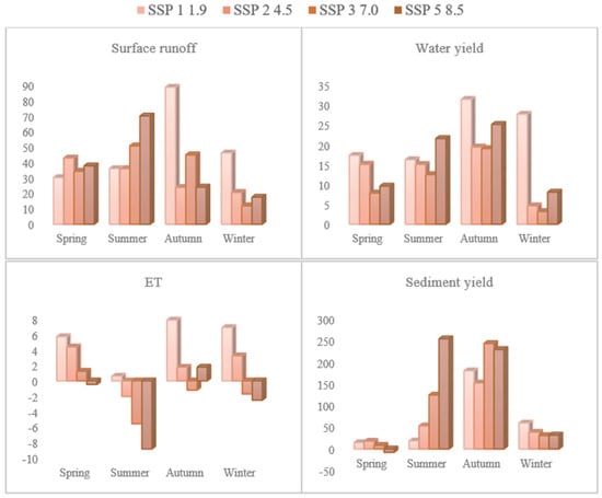
Figure 7.
Impacts of precipitation, temperature, and atmospheric [CO2] at seasonal scale (% change).
River Flow Parameters
The peaks of extreme low flows (<500 m3/s) will increase in the case of SSP 1, while it will decrease in other SSPs, with the largest decrease in SSP 5. The peaks of small floods (>10,000 m3/s) will increase across the SSPs with little difference, while the peaks of large floods (>14,000 m3/s) will increase largely in SSP 5 followed by 3 and 1. The duration of extreme low flows will decrease in case of SSP 1, while it will slightly increase in SSP 3 and 5. The duration of small floods will decrease across the SSPs, with the largest decrease in SSP 5 and 1. The duration of large floods will increase in the case of SSP 5, while it will decrease in the other SSPs. The frequency of extreme low flows will slightly decrease in the case of SSP 1, while it will increase in SSP 5. The frequency of small floods will increase across the SSPs with little difference. The frequency of large floods will increase across the SSPs with the largest increase in the case of SSP 5 followed by 3, 2, and 1. The minimum flows will increase largely in the case of SSP 1, while the maximum flows will increase across the SSPs with a greater increase in the case of SSP 5 (Figure 8).
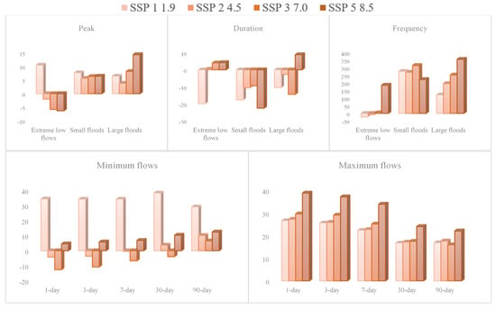
Figure 8.
Impacts on the river flow parameters (% change).
4. Discussion
The objectives of this study were to evaluate the individual and combined impacts of changes in three influencing factors, i.e., precipitation, temperature, and atmospheric CO2 concentration, for four future SSP scenarios. Individually, the impacts of changes in precipitation relative to temperature and carbon dioxide will be very large on all the studied hydrological parameters except ET. However, it is widely reported that global warming and elevated atmospheric CO2 concentration have opposing influence on plant transpiration [38,39]. Increased temperature enhances the biophysical driving force of transpiration, thereby contributing to increasing transpiration rates, while partial stomatal closure under elevated atmospheric CO2 concentration decreases the leaf loss of water [8,9,40]. Therefore, changes in the hydrological parameters in response to the combined impacts of the three influencing factors will be mostly associated with changes in precipitation.
Uncertainties in the precipitation data of the GCMs are widely reported [5,11,41,42,43]. Large uncertainties existed in precipitation data even after using the bias correction methods. The raw data of EC-Earth showed the highest agreement with the reference precipitation monthly time series; however, the similarity of the hydrological data obtained was not enough to simulate the actual future hydrology with minimum uncertainties, i.e., the data could not be compared to the observed historical hydrological data (Table 6 and Table 7). Therefore, we only extracted the difference between the historical and future hydrology; to minimize uncertainties among different GCMs, we used an ensemble mean or average of the precipitation data from four GCMs for SSP 2, 3, and 5, and from three GCMs for SSP 1, as discussed above. Extraction of the difference between the historical and future data of the GCMs does not minimize the uncertainties; however, it enables the impact studies to use the environment simulated by the GCM, i.e., rising greenhouse gases, etc. This method is widely used, and is known as delta change correction [42,44,45].

Table 6.
Mean values of the actual historical (1981–2014) basin hydrological data simulated using CMADs and GCMs precipitation data.

Table 7.
Mean values of the actual historical (1981–2014) river flow data simulated using CMADs and GCMs precipitation data.
The data of the GCMs of all the SSPs predicted increase in precipitation of the watershed. Increased precipitation will increase the surface runoff, water yield, and sediment yield. While using the GCMs data, several other studies reported an increase in future precipitation and runoff in watersheds around the globe [12,41,46,47]. The Minjiang river watershed is situated in a humid climate, and is an abundant fresh water resource. The abundant water resources of the watershed support several economic and social activities, such as electricity generation, recreation, and navigation. Increase in precipitation and water yield will increase the watershed’s capacity to support such activities. However, several ecological problems associated with precipitation, i.e., surface runoff, soil erosion, floods, and landslides, will become more intense.
Intense weather conditions have widespread harmful implications for natural systems and communities. Flash floods associated with storm runoff extremes are expected to become more frequent and severe due to climate change [48]. About 84% of the population in Fujian province is directly threatened by flash floods [49], and has experienced severe flash flood disasters. In our previous study [15], we found that surface runoff in the watershed increased during the recent past. Surface runoff will increase in the future. Increased surface runoff will enhance the damage risk during high-intensity precipitation and flood events in the watershed. Moreover, the water quality will deteriorate in the form of eutrophication due to more water flowing above the land surface into streams and rivers. This problem of surface runoff will be more severe in the case of the high carbon emission scenario (SSP 5), which is also predicted to exhibit the largest increase in large floods’ peaks, durations, and frequencies.
Each year, about 75 billion tons of soil is eroded from the world’s terrestrial ecosystems [50]. This is a severe challenge to the productivity of land [51]. The chemicals, contaminants, and heavy metals transported together with soil particles disturb the aquatic ecosystems by causing water eutrophication [52]. Moreover, sediment can reduce the storage capacity and disturb the operations of hydroelectric power plants [53]. In our previous study [15], we found that soil erosion in the watershed increased during the recent past. Soil erosion in the watershed is predicted to increase in the future. The problem of soil erosion will be more severe in the case of the low carbon emission scenario (SSP 1). The most likely reason is the substantial increase in winter precipitation because winter temperature is not suitable for plant growth and bare soil is more prone to erosion. Increase in temperature will decrease soil erosion to some extent, especially in the spring season of SSP 5, where despite increased water yield and surface runoff, sediment yield is simulated to decrease, most likely due to an increase in temperature.
Periodic water shortage is another most important and widely discussed hydrological problem that is commonly associated with future climate change. It was reported by the authors of [6] that future climate change can cause chronic and periodic water shortages. Our previous study [15] reported an increase in the severity of extreme low water yield in the Minjiang river watershed during the recent past. This study revealed that the problem of periodic water shortages (extreme low flows) in the watershed will become more severe in the future—except in the low carbon emission scenario (SSP 1)—in the form of intensity (peaks), duration, and occurrence (frequency).
5. Conclusions
Future climate change is expected to impact the natural systems around the globe. This study used future climate data of general circulation models of CMIP6 to investigate the impacts of climate change during the future period (2062–2095) relative to the historical period (1981–2014) on the hydrological system of the Minjiang river watershed. The soil and water assessment tool (SWAT) was employed to simulate the future hydrology under the impacts of changes in temperature, precipitation, and atmospheric [CO2] for four scenarios (SSP 1, 2, 3, and 5) of the CMIP6.
Several bias correction methods were used for downscaling of the GCM data. The temperature data of GCMs showed a great accuracy while the precipitation data showed large uncertainties. Bias correction performed differently for different GCMs and improved the accuracy of precipitation data to some extent. However, the accuracy was not enough to simulate the actual future hydrology with minimum uncertainties. Therefore, we only extracted the variation between the historical and future hydrology.
The results of the study revealed that the individual impacts of increase in future temperature, i.e., increased ET, and decrease in surface runoff, water, and sediment yield, will be countered by an increase in [CO2], and changes in the hydrological parameters in the future will be mostly associated with precipitation. Data of the GCMs for all the SSPs predicts increase in precipitation of the watershed, which will increase the surface runoff, water yield, and sediment yield. Evapotranspiration will increase only in SSP 1. Surface runoff will increase more in SSP 5, while sediment and water yield will increase more in SSP 1. On a seasonal scale, water yield and surface runoff will increase more in autumn and winter in SSP 1, while in other scenarios, these parameters will increase more in the spring and summer seasons. Sediment yield will increase more in autumn in all scenarios, while in it will increase more in summer in SSP 5 and in winter in SSP 1.
Similarly, the future climate change is predicted to impact the important parameters related to the flow regime of the Minjiang river, i.e., floods and extreme low flows. The frequency and duration of small floods (flows > 10,000 m3/s) will increase, while the duration will decrease in all scenarios with little difference. The frequency and peak of large floods (flows >14,000 m3/s) will increase along the gradient of scenarios, i.e., more in SSP 5 followed by 3, 2 and 1, while the duration will increase in SSP 5 and decrease in the other SSPs. The frequency and duration of extreme low flows will increase in SSP 5, while these parameters will decrease in SSP 1. Moreover, peak of extreme low flows will decrease in all scenarios except SSP 1, in which it will increase.
Author Contributions
S.L. conceived the idea and supervised the research; S.J. and A.Z. provided the materials, H.R. conducted the analysis and wrote the manuscript; K.Y. and A.R. helped in the study design and analysis; K.Y. and F.G. reviewed the manuscript. All authors have read and agreed to the published version of the manuscript.
Funding
The research was funded by “Funds for the Co-innovation Center for Soil and Water Conservation in Red Soil Region of the Cross-straits”, code K80ND8003.
Conflicts of Interest
The authors declare no conflict of interest.
References
- IPCC. The Physical Science Basis. Contribution of Working Group I to the Fifth Assessment Report of the Intergovernmental Panel on Climate Change; IPCC: Geneva, Switzerland, 2013. [Google Scholar]
- O’Neill, B.C.; Tebaldi, C.; van Vuuren, D.P.; Eyring, V.; Friedlingstein, P.; Hurtt, G.; Knutti, R.; Kriegler, E.; Lamarque, J.F.; Lowe, J.; et al. The Scenario Model Intercomparison Project (ScenarioMIP) for CMIP6. Geosci. Model Dev. 2016, 9, 3461–3482. [Google Scholar] [CrossRef] [Green Version]
- Taylor, K.E.; Stouffer, R.J.; Meehl, G.A. An Overview of CMIP5 and the Experiment Design. Bull. Am. Meteorol. Soc. 2012, 93, 485–498. [Google Scholar] [CrossRef] [Green Version]
- Mendez, M.; Maathuis, B.; Hein-Griggs, D.; Alvarado-Gamboa, L.-F. Performance Evaluation of Bias Correction Methods for Climate Change Monthly Precipitation Projections over Costa Rica. Water 2020, 12, 482. [Google Scholar] [CrossRef] [Green Version]
- IPCC. Climate Change 2021: The Physical Science Basis. In Contribution of Working Group I to the Sixth Assessment Report of the Intergovernmental Panel on Climate Change; Masson-Delmotte, V.P., Zhai, A., Pirani, S.L., Connors, C., Péan, S., Berger, N., Caud, Y., Chen, L., Goldfarb, M.I., Gomis, M., et al., Eds.; Cambridge University Press: Cambridge, UK, 2021. [Google Scholar]
- IPCC. Climate Change 2014: Synthesis Report. Contribution of Working Groups I, II and III to the Fifth Assessment Report of the Intergovernmental Panel on Climate Change; IPCC: Geneva, Switzerland, 2014. [Google Scholar]
- Teutschbein, C.; Seibert, J. Bias correction of regional climate model simulations for hydrological climate-change impact studies: Review and evaluation of different methods. J. Hydrol. 2012, 456, 12–29. [Google Scholar] [CrossRef]
- Butcher, J.B.; Johnson, T.E.; Nover, D.; Sarkar, S. Incorporating the effects of increased atmospheric CO2 in watershed model projections of climate change impacts. J. Hydrol. 2014, 513, 322–334. [Google Scholar] [CrossRef] [Green Version]
- Xu, Z.; Jiang, Y.; Jia, B.; Zhou, G. Elevated-CO2 Response of Stomata and Its Dependence on Environmental Factors. Front Plant Sci. 2016, 7, 657. [Google Scholar] [CrossRef] [Green Version]
- Arnold, J.; Moriasi, D.; Gassman, P.; Mikayilov, F.; White, M.; Srinivasan, R.; Santhi, C.; Harmel, R.; van Griensven, A.; Van Liew, M.; et al. SWAT: Model use, calibration, and validation. Trans. ASABE 2012, 55, 1491–1508. [Google Scholar] [CrossRef]
- Saddique, N.; Usman, M.; Bernhofer, C. Simulating the Impact of Climate Change on the Hydrological Regimes of a Sparsely Gauged Mountainous Basin, Northern Pakistan. Water 2019, 11, 2141. [Google Scholar] [CrossRef] [Green Version]
- Chanapathi, T.; Thatikonda, S. Investigating the impact of climate and land-use land cover changes on hydrological predictions over the Krishna river basin under present and future scenarios. Sci. Total Environ. 2020, 721, 137736. [Google Scholar] [CrossRef]
- Hyandye, C.B.; Worqul, A.; Martz, L.W.; Muzuka, A.N.N. The impact of future climate and land use/cover change on water resources in the Ndembera watershed and their mitigation and adaptation strategies. Environ. Syst. Res. 2018, 7, 7. [Google Scholar] [CrossRef] [Green Version]
- Wang, G.; Innes, J.L.; Hajjar, R.; Zhang, X.; Wang, J. Public Awareness and Perceptions of Watershed Management in the Min River Area, Fujian, China. Soc. Nat. Res. 2013, 26, 586–604. [Google Scholar] [CrossRef]
- Rashid, H.; Yang, K.; Zeng, A.; Ju, S.; Rashid, A.; Guo, F.; Lan, S. The Influence of Landcover and Climate Change on the Hydrology of the Minjiang River Watershed. Water 2021, 13, 3554. [Google Scholar] [CrossRef]
- Meng, X.; Wang, H.; Shi, C.; Wu, Y.; Ji, X. Establishment and Evaluation of the China Meteorological Assimilation Driving Datasets for the SWAT Model (CMADS). Water 2018, 10, 1555. [Google Scholar] [CrossRef] [Green Version]
- Meng, X.; Wang, H. Significance of the China Meteorological Assimilation Driving Datasets for the SWAT Model (CMADS) of East Asia. Water 2017, 9, 765. [Google Scholar] [CrossRef]
- Meng, X.; Wang, H.; Chen, J. Profound Impacts of the China Meteorological Assimilation Driving Datasets for the SWAT Model (CMADS). Water 2019, 11, 832. [Google Scholar] [CrossRef] [Green Version]
- FAO. Water for Sustainable Food and Agriculture; Food and Agriculture Organization of the United Nations: Rome, Italy, 2017. [Google Scholar]
- ESA. Land Cover CCI Product User Guide Version 2. 2017. Available online: https//:Maps.elie.ucl.ac.be/CCI/viewer/download/ESACCI-LC-Ph2-PUGv2_2.0.pdf (accessed on 7 March 2020).
- Moriasi, D.N.; Pai, N.; Steiner, J.L.; Gowda, P.H.; Winchell, M.; Rathjens, H.; Starks, P.J.; Verser, J.A. SWAT-LUT: A Desktop Graphical User Interface for Updating Land Use in SWAT. JAWRA 2019, 55, 1102–1115. [Google Scholar] [CrossRef] [Green Version]
- Abbaspour, K.C.; Vejdani, M.; Haghighat, S.; Yang, J. SWAT-CUP calibration and uncertainty programs for SWAT. In Proceedings of the MODSIM 2007 International Congress on Modelling and Simulation, Modelling and Simulation Society of Australia and New Zealand, Christchurch, New Zealand, 10–13 December 2007; pp. 1596–1602. [Google Scholar]
- Moriasi, D.N.; Arnold, J.G.; Van Liew, M.W.; Bingner, R.L.; Harmel, R.D.; Veith, T.L. Model Evaluation Guidelines for Systematic Quantification of Accuracy in Watershed Simulations. Trans. ASABE 2007, 50, 885–900. [Google Scholar] [CrossRef]
- Eyring, V.; Bony, S.; Meehl, G.A.; Senior, C.A.; Stevens, B.; Stouffer, R.J.; Taylor, K.E. Overview of the Coupled Model Intercomparison Project Phase 6 (CMIP6) experimental design and organization. Geosci. Model Dev. 2016, 9, 1937–1958. [Google Scholar] [CrossRef] [Green Version]
- Peano, D.; Lovato, T.; Materia, S. CMCC CMCC-ESM2 Model Output Prepared for CMIP6 LS3MIP; Earth System Grid Federation: Italy, 2020; Available online: https://cera-www.dkrz.de/WDCC/ui/cerasearch/cmip6?input=CMIP6.LS3MIP.CMCC.CMCC-ESM2 (accessed on 22 September 2021).
- Zhang, J.; Wu, T.; Shi, X.; Zhang, F.; Li, J.; Chu, M.; Liu, Q.; Yan, J.; Ma, Q.; Wei, M. BCC BCC-ESM1 Model Output Prepared for CMIP6 CMIP Historical. 2018. Available online: https://cera-www.dkrz.de/WDCC/ui/cerasearch/cmip6?input=CMIP6.CMIP.BCC.BCC-ESM1.historical (accessed on 22 September 2021).
- Bi, D.; Dix, M.R.; Marsland, S.J.; O’Farrell, S.P.; Rashid, H.A.; Uotila, P.; Hirst, A.C.; Kowalczyk, E.A.; Golebiewski, M.; Sullivan, A.; et al. The ACCESS coupled model: Description, control climate and evaluation. Aust. Meteorol. Oceanogr. J. 2013, 63, 41–64. [Google Scholar] [CrossRef]
- Pu, Y.; Liu, H.; Yan, R.; Yang, H.; Xia, K.; Li, Y.; Dong, L.; Li, L.; Wang, H.; Nie, Y.; et al. CAS FGOALS-g3 Model Datasets for the CMIP6 Scenario Model Intercomparison Project (ScenarioMIP). Adv. Atmos. Sci. 2020, 37, 1081–1092. [Google Scholar] [CrossRef]
- Swart, N.C.; Cole, J.N.S.; Kharin, V.V.; Lazare, M.; Scinocca, J.F.; Gillett, N.P.; Anstey, J.; Arora, V.; Christian, J.R.; Jiao, Y.; et al. CCCma CanESM5 Model Output Prepared for CMIP6 CMIP Historical. 2019. Available online: https://cera-www.dkrz.de/WDCC/ui/cerasearch/cmip6?input=CMIP6.CMIP.CCCma.CanESM5.historical (accessed on 22 September 2021).
- Mauritsen, T.; Bader, J.; Becker, T.; Behrens, J.; Bittner, M.; Brokopf, R.; Brovkin, V.; Claussen, M.; Crueger, T.; Esch, M.; et al. Developments in the MPI-M Earth System Model version 1.2 (MPI-ESM1.2) and Its Response to Increasing CO2. J. Adv. Model. Earth Syst. 2019, 11, 998–1038. [Google Scholar] [CrossRef] [PubMed] [Green Version]
- Wu, T.; Chu, M.; Dong, M.; Fang, Y.; Jie, W.; Li, J.; Li, W.; Liu, Q.; Shi, X.; Xin, X.; et al. BCC BCC-CSM2MR Model Output Prepared for CMIP6 CMIP Historical. 2018. Available online: https://cera-www.dkrz.de/WDCC/ui/cerasearch/cmip6?input=CMIP6.CMIP.BCC.BCC-CSM2-MR.historical (accessed on 22 September 2021).
- Tatebe, H.; Ogura, T.; Nitta, T.; Komuro, Y.; Ogochi, K.; Takemura, T.; Sudo, K.; Sekiguchi, M.; Abe, M.; Saito, F.; et al. Description and basic evaluation of simulated mean state, internal variability, and climate sensitivity in MIROC6. Geosci. Model Dev. 2019, 12, 2727–2765. [Google Scholar] [CrossRef] [Green Version]
- Consortium, E.C.-E. EC-Earth-Consortium EC-Earth3-Veg-LR Model Output Prepared for CMIP6 CMIP Historical. 2020. Available online: https://cera-www.dkrz.de/WDCC/ui/cerasearch/cmip6?input=CMIP6.CMIP.EC-Earth-Consortium.EC-Earth3-Veg-LR.historical (accessed on 22 September 2021).
- Yukimoto, S.; Koshiro, T.; Kawai, H.; Oshima, N.; Yoshida, K.; Urakawa, S.; Tsujino, H.; Deushi, M.; Tanaka, T.; Hosaka, M.; et al. MRI MRI-ESM2.0 Model Output Prepared for CMIP6 CMIP Historical. 2019. Available online: https://cera-www.dkrz.de/WDCC/ui/cerasearch/cmip6?input=CMIP6.CMIP.MRI.MRI-ESM2-0.historical (accessed on 22 September 2021).
- Rathjens, H.; Bieger, K.; Srinivasan, R.; Arnold, J. CMhyd User Manual: Documentation for Preparing Simulated Climate Change Data for Hydrologic Impact Studies. 2016. Available online: https://cds.climate.copernicus.eu (accessed on 22 September 2021).
- Morison, J.I.L. Intercellular CO2 concentration and stomatal response to CO2. Stomatal Funct. 1987, 10, 229–251. [Google Scholar]
- Neitsch, S.; Arnold, J.; Kinry, J.R.; Williams, J.R. Soil and Water Assessment Tool Theoretical Documentation Version 2011; Texas Water Resources Institute: College Station, TX, USA, 2011. [Google Scholar]
- Kirschbaum, M.U.F.; McMillan, A.M.S. Warming and Elevated CO2 Have Opposing Influences on Transpiration. Which is more Important? Curr. For. Rep. 2018, 4, 51–71. [Google Scholar] [CrossRef] [Green Version]
- Gedney, N.; Cox, P.M.; Betts, R.A.; Boucher, O.; Huntingford, C.; Stott, P.A. Detection of a direct carbon dioxide effect in continental river runoff records. Nature 2006, 439, 835–838. [Google Scholar] [CrossRef]
- Field, C.B.; Jackson, R.B.; Mooney, H.A. Stomatal responses to increased CO2: Implications from the plant to the global scale. Plant Cell Environ. 1995, 18, 1214–1225. [Google Scholar] [CrossRef]
- Mahmood, R.; Jia, S. Assessment of Impacts of Climate Change on the Water Resources of the Transboundary Jhelum River Basin of Pakistan and India. Water 2016, 8, 246. [Google Scholar] [CrossRef] [Green Version]
- Yang, K.; Lu, C. Evaluation of land-use change effects on runoff and soil erosion of a hilly basin—The Yanhe River in the Chinese Loess Plateau. Land Degrad. Dev. 2018, 29, 1211–1221. [Google Scholar] [CrossRef]
- Zhang, S.; Chen, J.; Gu, L. Overall uncertainty of climate change impacts on watershed hydrology in China. Int. J. Climatol. 2021. [Google Scholar] [CrossRef]
- Navarro-Racines, C.; Tarapues, J.; Thornton, P.; Jarvis, A.; Ramirez-Villegas, J. High-resolution and bias-corrected CMIP5 projections for climate change impact assessments. Sci. Data 2020, 7, 7. [Google Scholar] [CrossRef] [PubMed] [Green Version]
- Haider, H.; Zaman, M.; Liu, S.; Saifullah, M.; Usman, M.; Chauhdary, J.N.; Anjum, M.N.; Waseem, M. Appraisal of Climate Change and Its Impact on Water Resources of Pakistan: A Case Study of Mangla Watershed. Atmosphere 2020, 11, 1071. [Google Scholar] [CrossRef]
- Sha, J.; Zhao, Y.; Li, X.; Wang, Z.-l. Assessing impacts of future climate change on hydrological processes in an urbanizing watershed with a multimodel approach. J. Water Clim. Chang. 2020, 12, 1023–1042. [Google Scholar] [CrossRef]
- Pokhrel, P.; Ohgushi, K.; Fujita, M. Impacts of future climate variability on hydrological processes in the upstream catchment of Kase River basin, Japan. Appl. Water Sci. 2019, 9, 18. [Google Scholar] [CrossRef] [Green Version]
- Yin, J.; Gentine, P.; Zhou, S.; Sullivan, S.C.; Wang, R.; Zhang, Y.; Guo, S. Large increase in global storm runoff extremes driven by climate and anthropogenic changes. Nat. Commun. 2018, 9, 4389. [Google Scholar] [CrossRef] [Green Version]
- Cao, Y.; Jia, H.; Xiong, J.; Cheng, W.; Li, K.; Pang, Q.; Yong, Z. Flash Flood Susceptibility Assessment Based on Geodetector, Certainty Factor, and Logistic Regression Analyses in Fujian Province, China. ISPRS Int. J. Geo-Inf. 2020, 9, 748. [Google Scholar] [CrossRef]
- Durán Zuazo, V.H.; Rodríguez Pleguezuelo, C.R. Soil-erosion and runoff prevention by plant covers. A review. Agron. Sustain. Dev. 2008, 28, 65–86. [Google Scholar] [CrossRef] [Green Version]
- FAO. Soil Erosion: The Greatest Challenge to Sustainable Soil Management; Food and Agriculture Organization of the United Nation: Rome, Italy, 2019; p. 100. [Google Scholar]
- Issaka, S.; Ashraf, M.A. Impact of soil erosion and degradation on water quality: A review. Geol. Ecol. Landsc. 2017, 1, 1–11. [Google Scholar] [CrossRef] [Green Version]
- Kondolf, G.M.; Gao, Y.; Annandale, G.W.; Morris, G.L.; Jiang, E.; Zhang, J.; Cao, Y.; Carling, P.; Fu, K.; Guo, Q.; et al. Sustainable sediment management in reservoirs and regulated rivers: Experiences from five continents. Earths Future 2014, 2, 256–280. [Google Scholar] [CrossRef]
Publisher’s Note: MDPI stays neutral with regard to jurisdictional claims in published maps and institutional affiliations. |
© 2021 by the authors. Licensee MDPI, Basel, Switzerland. This article is an open access article distributed under the terms and conditions of the Creative Commons Attribution (CC BY) license (https://creativecommons.org/licenses/by/4.0/).