Cluster and Redundancy Analyses of Taiwan Upstream Watersheds Based on Monthly 30 Years AVHRR NDVI3g Data

Abstract

The study uses 30 years of the third generation of Advanced Very-High-Resolution Radiometer (AVHRR) NDVI3g monthly data from 1982 to 2012 to identify the natural clusters and important driving factors of the upstream watersheds in Taiwan through hierarchical cluster analysis (HCA) and redundancy analysis (RDA), respectively. Subsequently, as a result of HCA, six clusters were identified based on the 30 years of monthly NDVI data, delineating unique NDVI characteristics of the upstream watersheds. Additionally, based on the RDA results, environmental factors, including precipitation, temperature, slope, and aspect, can explain approximately 52% of the NDVI variance over the entire time series. Among environmental factors, nine factors were identified significantly through RDA analysis for explaining NDVI variance: average slope, temperature, flat slope, northeast-facing slope, rainfall, east-facing slope, southeast-facing slope, west-facing slope, and northwest-facing slope, which reflect an intimate connection between climatic and orthographic factors with vegetation. Furthermore, the rainfall and temperature represent different variations in all scenarios and seasons. With consideration of the characteristics of the clusters and significant environmental factors, corresponding climate change adaptation strategies are proposed for each cluster under climate change scenarios. Thus, the results provide insight to assess the natural clustering of the upstream watersheds in Taiwan, benefitting future sustainable watershed management.

1. Introduction

Upstream watersheds play a critical role in the regional hydrologic system and are sensitive to climate change [1]. For instance, the upstream watersheds usually comprise high mountains containing the headwater zone in a river system [2]. The headwater zone is vital for understanding and protecting downstream ecosystems because they are intimately linked based on interactions among hydrologic, geomorphic, and biological processes [3]. Thus, a hydrological event in an upstream watershed may directly influence downstream areas many hundreds of kilometers away, highlighting the crucial ecological role of the upstream watersheds [2]. Additionally, compared with downstream areas, upstream watersheds generally comprise high mountains, steep gradients, and high ridges, thus resulting in low accessibilities and less human interventions. As upstream watersheds are relatively unaffected by human interventions, the changes observed in upstream watersheds indicate effects of climate change [4].

The effects of climate change in the upstream watersheds are studied extensively worldwide. Some scholars focus on runoff variations [5,6], while others study river flow regimes [7], streamflows [8,9], and reservoir flood control [10], and so on. Among the studies of climate change effects, several authors have investigated the response of vegetation in the upstream watersheds [11,12]. Further studies of future climate variability impacts on hydrological processes can also be assessed through vegetation responses [13,14].

The roles of vegetation cover in the upstream watershed can be discussed from many relevant aspects, such as evapotranspiration, infiltration, soil erosion, and runoff, etc. [2]. First of all, forests in the upstream watershed ordinarily influence local hydrology through evapotranspiration. Additionally, forests in the upstream watershed also affect infiltration processes into underlying soil and ground cover through their root systems and organic humus layer, controlling soil erosion dynamics, runoff mechanisms, and landslides on sloping land [15,16,17]. In short, vegetation plays an important role in the energy exchanges, biogeochemical cycles, and hydrological cycles at the land surface [11,18]. Thus, the phenological response of vegetation in the upstream watershed is an environmental indicator because vegetation constitutes the foundation of the terrestrial ecosystem and denotes a natural connection among the atmosphere, water, and soil.

In the West Pacific, Taiwan is a unique island with over 60% of its land covered by high mountains with maximum altitudes of 4000 m. East Asian monsoon systems and typhoons play a major domination role on the precipitation patterns in Taiwan. Coupled with the Central Mountain Range (CMR), Taiwan’s precipitation patterns are complex, with extensive local variations [19]. In addition, Taiwan is characterized by geological weakness with frequent seismic activities resulting in the high vulnerability of Taiwan [20]. In recent years, Taiwan has encountered increasing pressure from various extreme climate events due to global climate change, such as severe drought [21,22,23], intensive typhoons [24], and associated natural disasters [25]. Almost all extreme climate occasions are related to water-based situations. For instance, heavy rainfall events have become more frequent and concentrated, leading to disasters such as landslides and debris flow in many watersheds locating at the upstream area, which have seriously affected the safety of the people [26,27,28]. In August 2009, Typhoon Morakot brought record-breaking heavy rainfall to the upstream watershed in southwestern and southeastern Taiwan. Numerous landslides and debris flow were triggered by the heavy rainfall of nearly 2000 mm within five days, which makes the number of life losses ranks second in the history of Taiwan’s natural disasters behind the Chi-Chi earthquake in 1999 [29]. The increases in climatic abnormalities and potential impacts, relevant national policies, and further environmental studies were employed and emerged for enhancing hazard remediation, mitigation, prediction, prevention plans for Taiwan’s upstream watershed [30,31,32,33,34,35,36].

Remote sensing techniques have been used for large-scale environmental studies due to their broad spatial coverage and regular revisit capacities. The normalized difference vegetation index (NDVI) is the most widely used remote sensing-derived satellite-based vegetation index. Numerous studies utilize continuous NDVI time-series data to analyze the relationship between vegetation and climatic factors such as rainfall, temperature, sunshine duration, and cloud amount [37,38,39,40,41]. Tsai et al. [42] analyze Taiwan’s spatial vegetation trends with controlling environmental variables, including temperature, precipitation, slope, aspects, and population density, based on the three-decades-long Advanced Very-High-Resolution Radiometer (AVHRR) NDVI3g data from 1982 to 2012 derived from 19 selected weather stations. Additionally, many scholars use NDVI to investigate natural disaster responses such as landslides in Taiwan [43,44,45]. Nevertheless, most studies focus on a specific time frame/area or use data from selected weather stations. A long-term holistic assessment of the vegetation and climatic characteristics in the upstream watersheds is of great importance for discerning the effect of climate change in the upstream watersheds in Taiwan.

Therefore, the present study assesses the long-term vegetation and environmental characteristics in the upstream watersheds of Taiwan from a broader watershed scale using long-term remote sensed vegetation index NDVI, climatic factors temperature and precipitation, and orographic factors aspect and slope. Specifically, the hierarchical cluster (HCA) and redundancy (RDA) analyses discern natural clusters based on monthly NDVI data and important driving factors of long-term changes in vegetation greenness, respectively. Moreover, in future climate change scenarios, corresponding comprehensive adaptation strategies are proposed for the upstream watershed clusters. Consequently, the results of this study may benefit disaster prevention and watershed management by a holistically understanding of upstream watersheds and their possible future impacts under different climate scenarios.

2. Materials and Methods

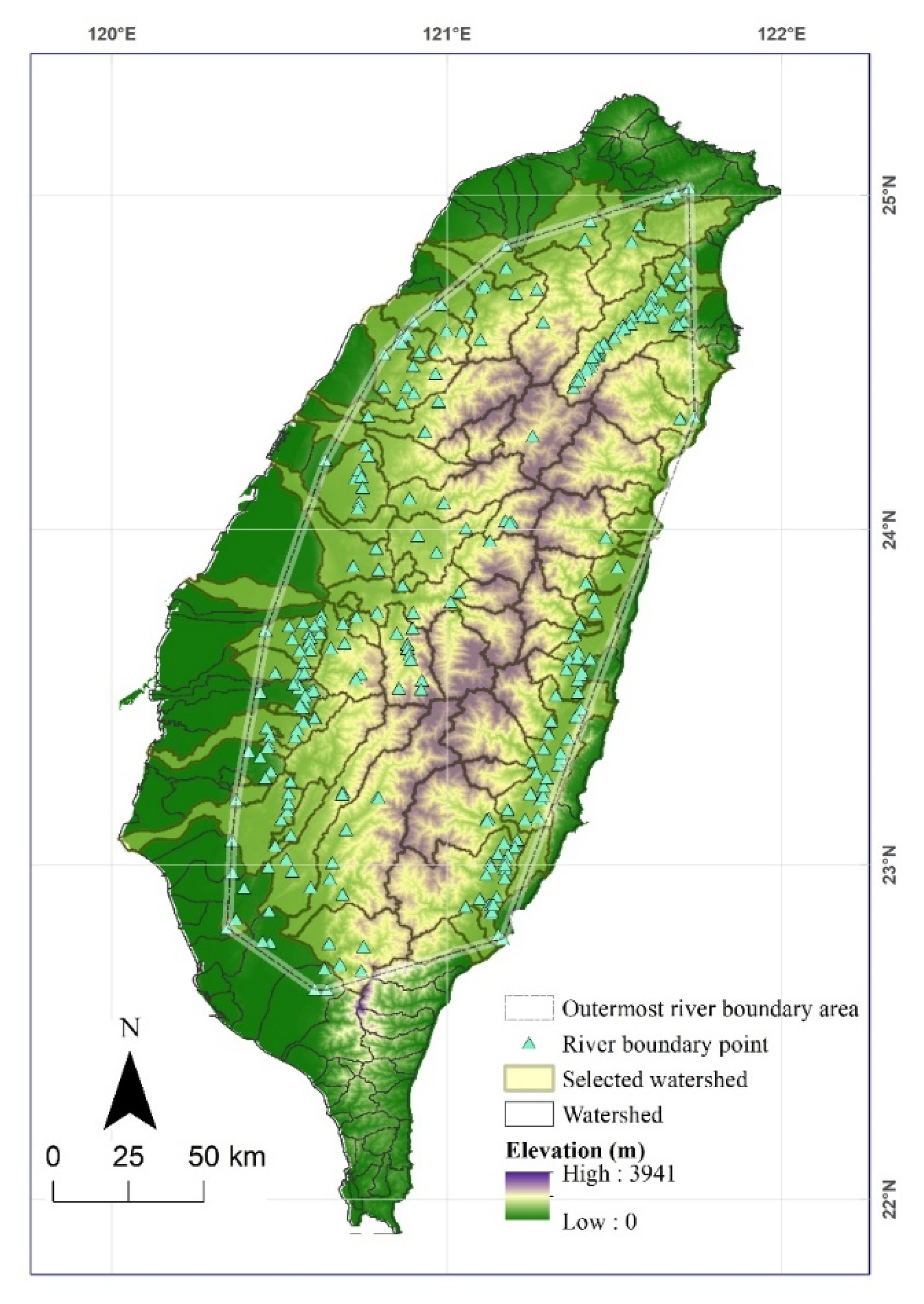
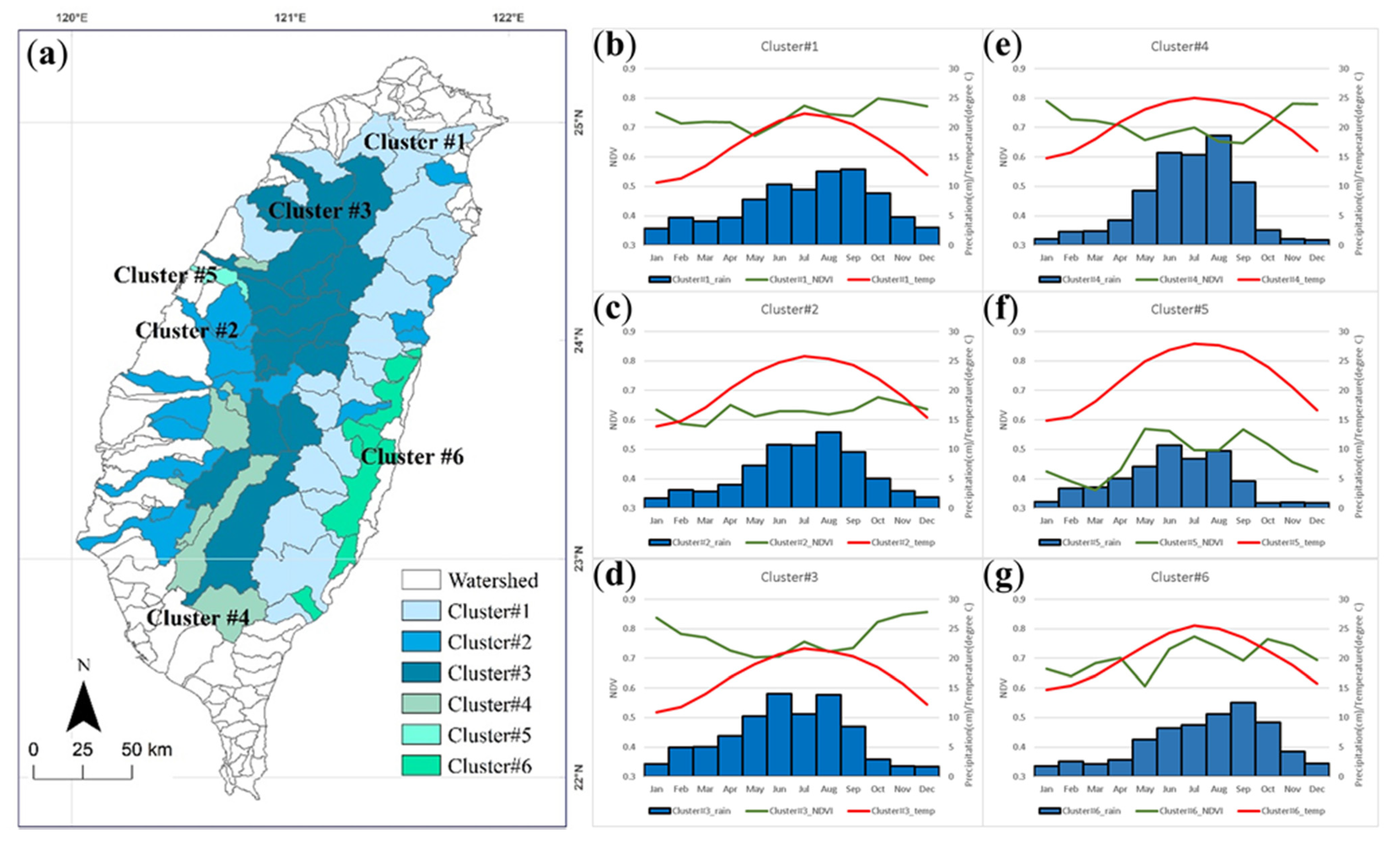
2.1. Study Area

The definition of upstream watersheds is not well-defined in Taiwan’s Soil and Water Conservation Act. In general, a large river basin comprises several secondary watersheds, with the area being much smaller. As the spatial resolution of the remote sensed vegetation data used in this study is 8 × 8 km; therefore, this study uses the secondary watersheds (from now on referred to as the “watershed”). Additionally, the river boundary points (Figure A1) announced by Taiwan’s Soil and Water Conservation Bureau to determine the central government administration area are used to determine Taiwan’s upstream watershed. Given the distribution of the river boundary points, the outermost river boundary points are linked to depict a conceptual outermost river boundary area (Figure A1). Then, the upstream watersheds are determined as the central point of the watershed to be within this conceptual outermost river boundary area. At present, 70 watersheds, encompassing approximately 67.3% of Taiwan, were selected as the upstream watersheds for subsequent analysis. The upstream watersheds are demonstrated in Figure A1 in the Appendix B, and the detailed information is shown in

Table A1. List of selected watershed.

#	Serial Number of Watershed	City/County	Name of River Basin	Name of Watershed	Area of Watershed (km2)
1	1002	Taichung City	Dajia River	Guguan adjustment pool	196.12
2	1204	Nantou County	Zhuoshui River	Shuili river	58.03
3	1504	Chiayi County	Bazhang River	Luliao reservoir	8.48
4	1704	Tainan County	Zengwen River	Jingmian reservoir	16.24
5	2505	Hualien County	Xiuguluan River	Xiuguluan river	200.54
6	2607	Hualien County	Hualien River	Ji-an river	35.02
7	0101	Yilan County	Lanyang River	Lanyang river	932.65
8	0102	Yilan County	Lanyang River	Yilan river	187.72
9	0401	Hsinchu County	Tamsui River	Shimen reservoir	835.90
10	0402	New Taipei City	Tamsui River	Feitsui reservoir	328.80
11	0403	Taoyuan City	Tamsui River	Dahan river	451.85
12	0404	New Taipei City	Tamsui River	Hsindian river	541.30
13	0501	Hsinchu County	Fengshan River	Fengshan river	277.73
14	0601	Hsinchu County	Touchian River	Touchian river	626.72
15	0701	Miaoli County	Zhonggang River	Zhonggang river	375.61
16	0702	Hsinchu County	Zhonggang River	Dapu reservoir	121.51
17	0801	Miaoli County	Houlong River	Houlong river	526.84
18	0802	Miaoli County	Houlong River	Mingde reservoir	88.74
19	0901	Miaoli County	Daan River	Daan river	765.56
20	0902	Miaoli County	Daan River	Liyutan reservoir	81.97
21	1001	Taichung City	Dajia River	Deji reservoir	574.86
22	1003	Taichung City	Dajia River	Tianlun adjustment pool	93.30
23	1004	Taichung City	Dajia River	Shigang reservoir	344.74
24	1005	Taichung City	Dajia River	Dajia river	163.71
25	1101	Taichung City	Wu River	Beigang river	565.48
26	1102	Nantou County	Wu River	Nangang river	473.49
27	1104	Taichung City	Wu River	Dali river	433.64
28	1105	Changhua County	Wu River	Maoluo river	407.12
29	1106	Changhua County	Wu River	Wu river	229.14
30	1201	Nantou County	Zhuoshui River	Wushe reservoir	245.89
31	1202	Nantou County	Zhuoshui River	Wujie adjustment pool	368.04
32	1203	Nantou County	Zhuoshui River	Sun Moon Lake reservoir	33.75
33	1205	Yunlin County	Zhuoshui River	Zhuoshui river	771.10
34	1206	Nantou County	Zhuoshui River	Danda river	294.12
35	1207	Nantou County	Zhuoshui River	Junda river	455.64
36	1208	Nantou County	Zhuoshui River	Chenyoulan river	490.91
37	1209	Chiayi County	Zhuoshui River	Qingshui river	462.69
38	1210	Nantou County	Zhuoshui River	Kashe river	183.99
39	1211	Nantou County	Zhuoshui River	Dongpuna river	109.24
40	1301	Yunlin County	Beigang River	Huwei river	332.03
41	1302	Yunlin County	Beigang River	Sandie river	209.73
42	1501	Chiayi County	Bazhang River	Bazhang river	460.98
43	1601	Chiayi County	Jishui river	Baihe reservoir	38.69
44	1701	Kaoshiung City	Zengwen River	Zengwen reservoir	519.83
45	1702	Tainan City	Zengwen River	Wushantou reservoir	70.29
46	1703	Tainan City	Zengwen River	Nanhua reservoir	138.94
47	1705	Tainan City	Zengwen River	Zengwen river	624.05
48	2101	Kaoshiung City	Kaoping River	Qishan river	819.68
49	2102	Kaoshiung City	Kaoping River	Laonong river	1537.71
50	2103	Pingtung County	Kaoping River	Ailiao river	678.61
51	2401	Taitung County	Beinan River	Beinan river	1017.08
52	2402	Taitung County	Beinan River	Hsinwulue river	733.84
53	2501	Hualien County	Hsiuguluan River	Hsiuguluan river	765.36
54	2502	Hualien County	Hsiuguluan River	Hsiuguluan river	190.30
55	2503	Hualien County	Hsiuguluan River	Hsiuguluan river	494.19
56	2504	Hualien County	Hsiuguluan River	Hsiuguluan river	313.83
57	2601	Hualien County	Hualien River	Hualien river coastal area	503.83
58	2602	Hualien County	Hualien River	Maan river	173.83
59	2603	Hualien County	Hualien River	Wanli river	267.11
60	2604	Hualien County	Hualien River	Shoufeng river	236.08
61	2605	Hualien County	Hualien River	Mugua river	486.47
62	2606	Hualien County	Hualien River	Meilun river	101.20
63	2701	Hualien County	Heping River	Heping river	629.64
64	2703	Yilan County	Heping River	Nanao river	361.65
65	4301	Taitung County	River system of Taitung coastal area	Taiping river	120.61
66	4302	Taitung County	River system of Taitung coastal area	Lichia river	194.73
67	4403	Taitung County	Rivers on the east side of the Coastal Mountains	Mawu river	163.43
68	4601	Hualien County	River system of Taroko coastal area	Kanaan coastal area	98.88
69	4602	Hualien County	River system of Taroko coastal area	Liwu river	693.63
70	4603	Hualien County	River system of Taroko coastal area	Shanzhan river	149.79

in the Appendix A.

2.2. Research Procedure

The research procedure of this study is shown in Figure 1. Firstly, the upstream watersheds were determined based on the river boundary information. The terrain information slope and aspect were then collected. Next, the monthly NDVI, temperature, and rainfall data from 1982 to 2012 were collected. Subsequently, the cluster analysis for the upstream watershed and identifying the driving factors (slope, aspect, temperature, and rainfall) was conducted based on the collected data. The important driving factors then investigated the variation of the clustered upstream watersheds under the four climate change scenarios. Finally, the adaption strategies for the climate change of each cluster were proposed.

2.3. Data Acquisition

2.3.1. Normalized Difference Vegetation Index

The present study utilized a high temporal resolution (15 days) of NDVI dataset, which is the third generation of Advanced Very-High-Resolution Radiometer (AVHRR) NDVI3g exploited by the Global Inventory Modeling and Mapping Studies (GIMMS) group [46]. The dataset’s spatial resolution is 1/12 degree (approximately 8 km), and the period spans from January 1982 to December 2012. A series of AVHRR sensors produce the AVHRR NDVI3g dataset in the GIMMS project framework at the National Aeronautics and Space Administration (NASA) Goddard Space Flight Center. The AVHRR NDVI3g dataset has been corrected for atmospheric scattering, volcanic eruptions, and the effects of cloud cover [47,48,49]. Furthermore, by using the maximum value composition method [49,50], the 15-day NDVI3g data are combined from the daily data to reduce cloud and aerosol contamination [51]. Currently, the AVHRR NDVI3g dataset is the NDVI dataset that is available for providing vegetation cover globally with the most prolonged period. This situation offers an extraordinary opportunity to analyze long-term vegetation configuration. In this study, the maximum NDVI values from January 1982 to December 2012 were obtained from the NDVI3g dataset for each watershed’s NDVI time series material.

2.3.2. Temperature and Rainfall

Precipitation and temperature data from 1982 to 2012 were obtained from the Taiwan Climate Change Projection and Information Platform (TCCIP) at a monthly time scale in a raster format. The TCCIP datasets were produced based on observations derived from more than 1152 weather station data since 1960. Using the inverse distance weighted interpolation and weighted average methods suggested in [52], the TCCIP datasets were produced at 5 × 5 km² spatial resolution.

2.3.3. Slope and Aspect

Slope and aspect data were produced from the 40 m × 40 m digital terrain model (DTM) made by the Taiwan Ministry of the Interior. The aspects included flat aspect (Flat), north aspect (N), northeast aspect (NE), east aspect (E), southeast aspect (SE), south aspect (S), southwest aspect (SW), west aspect (W), and northwest aspect (NW). Detailed slope and aspect data were extracted for the watershed area in Taiwan using ArcGIS software (Version 10.6.1 Redlands, CA, USA: Environmental Systems Research Institute, Inc., 2019).

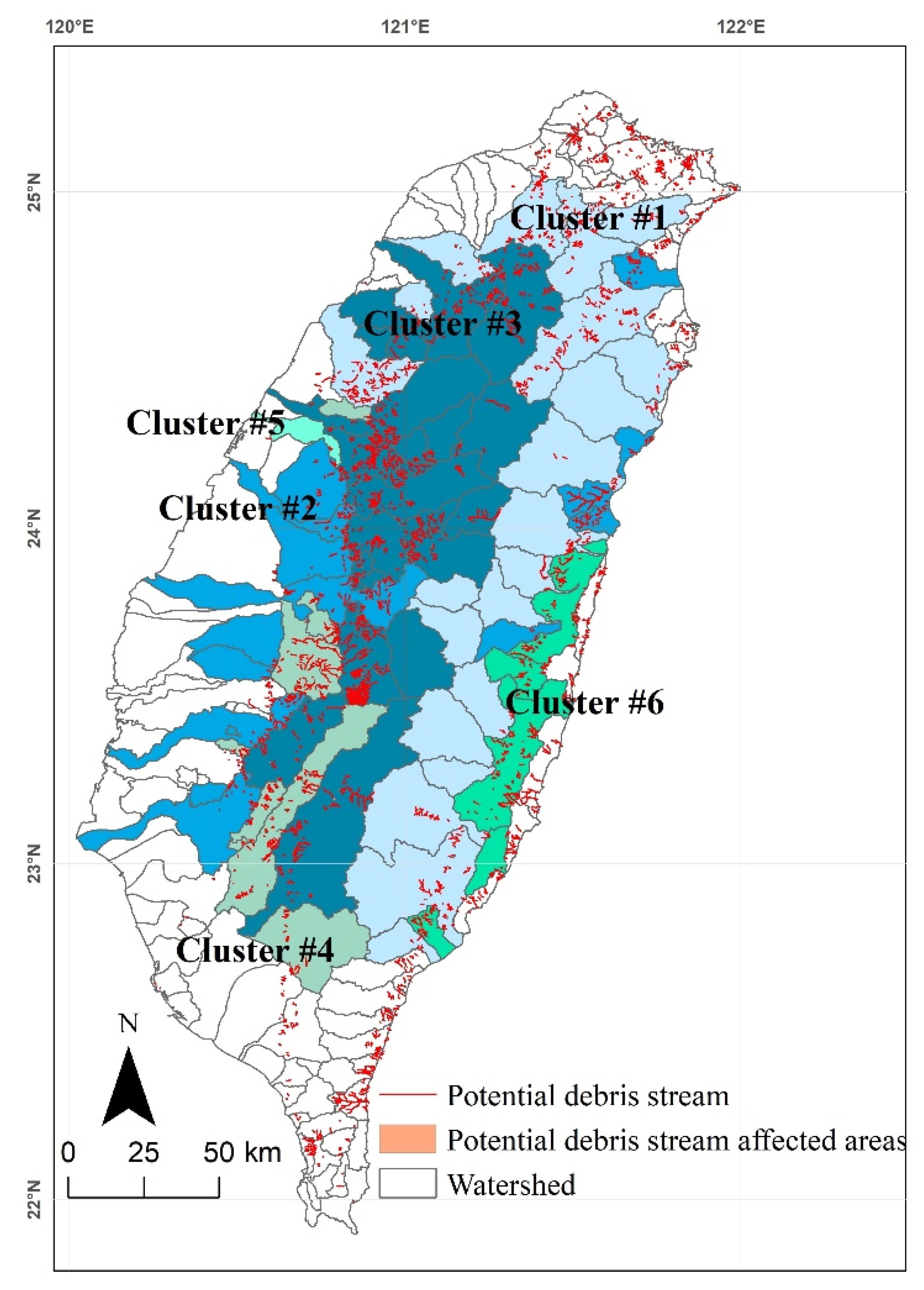
2.3.4. Potential Debris Streams and Affected Area

The potential debris streams and affected area information were collected from Taiwan’s Soil and Water Conservation Bureau. The total number of potential debris streams in Taiwan is 1726, while 1863 sites were recognized as the area affected by potential debris streams. The cluster results were overlapped with the potential debris streams and affected areas for further discussion.

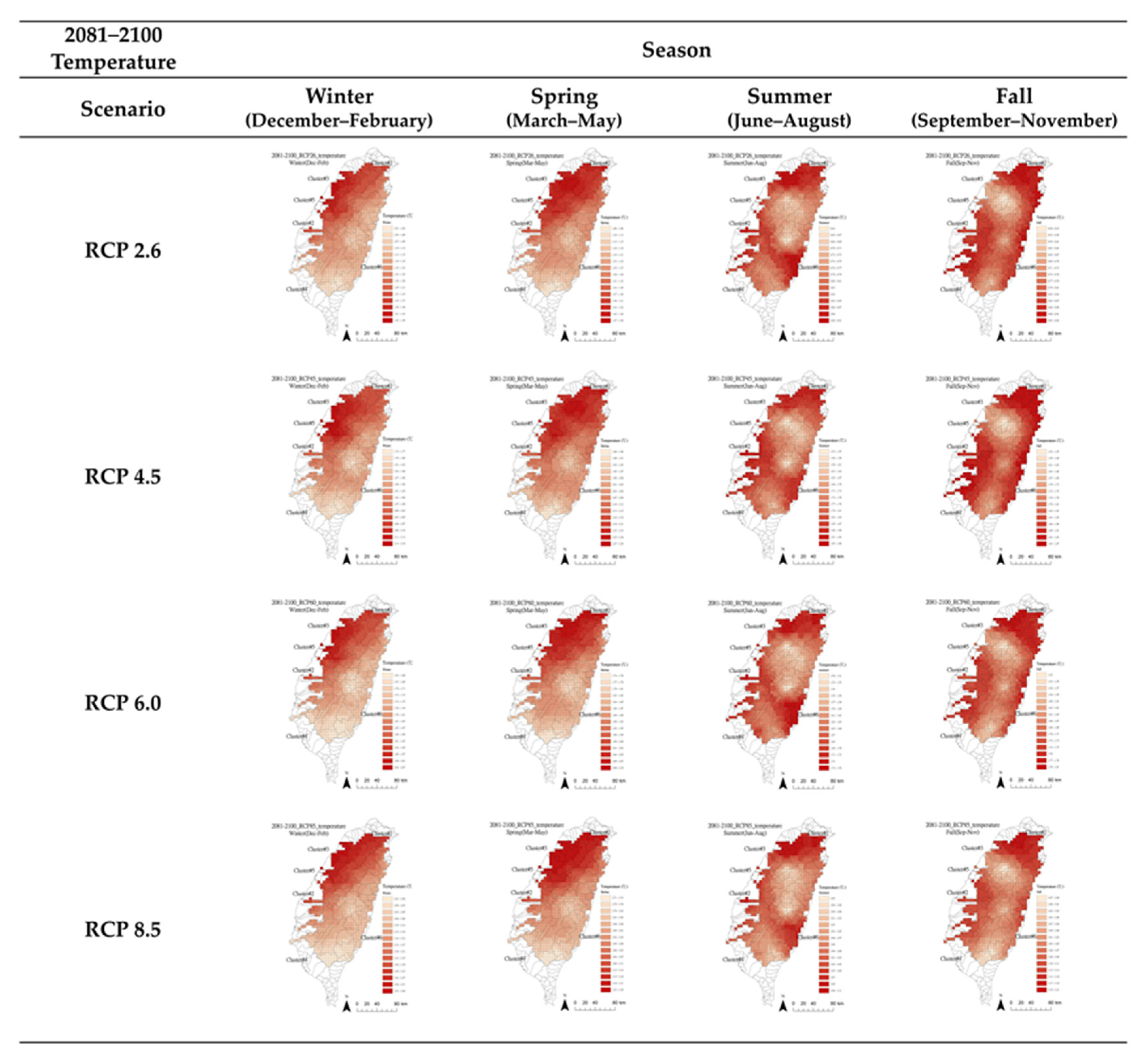
2.3.5. Climate Change Scenarios

This study obtains the simulated monthly temperature and rain change rate from the TCCIP [53] from 2021 to 2100. The data represent near to distant future under the evaluation of the Representative Concentration Pathways (RCPs), describe the 21st-century pathways of greenhouse gas emissions and atmospheric concentrations, air pollutant emissions, and land use driven by human activities [54]. Four different climate change scenarios, RCP2.6, RCP4.5, RCP6.0, and RCP8.5, representing the global temperature rising level from 2 °C to severe warming, have been reported in the fifth assessment report (AR5) of the Intergovernmental Panel on Climate Change (IPCC).

Among various atmosphere-ocean general circulation models, Lin and Tung [55] suggested using the Hadley Global Environment Model 2 (HadGEM2-AO) developed by the National Institute of Meteorological Research, Seoul, South Korea. Indeed, it is suitable to estimate the rainfall variation ratio (%) and temperature variation value (°C) in Taiwan. Hence, the HadGEM2-AO is chosen to discuss climate change scenarios, focusing on the temperature and rainfall variations of the watersheds from 2021 to 2100 in Section 3.5.

2.4. Statistics Models

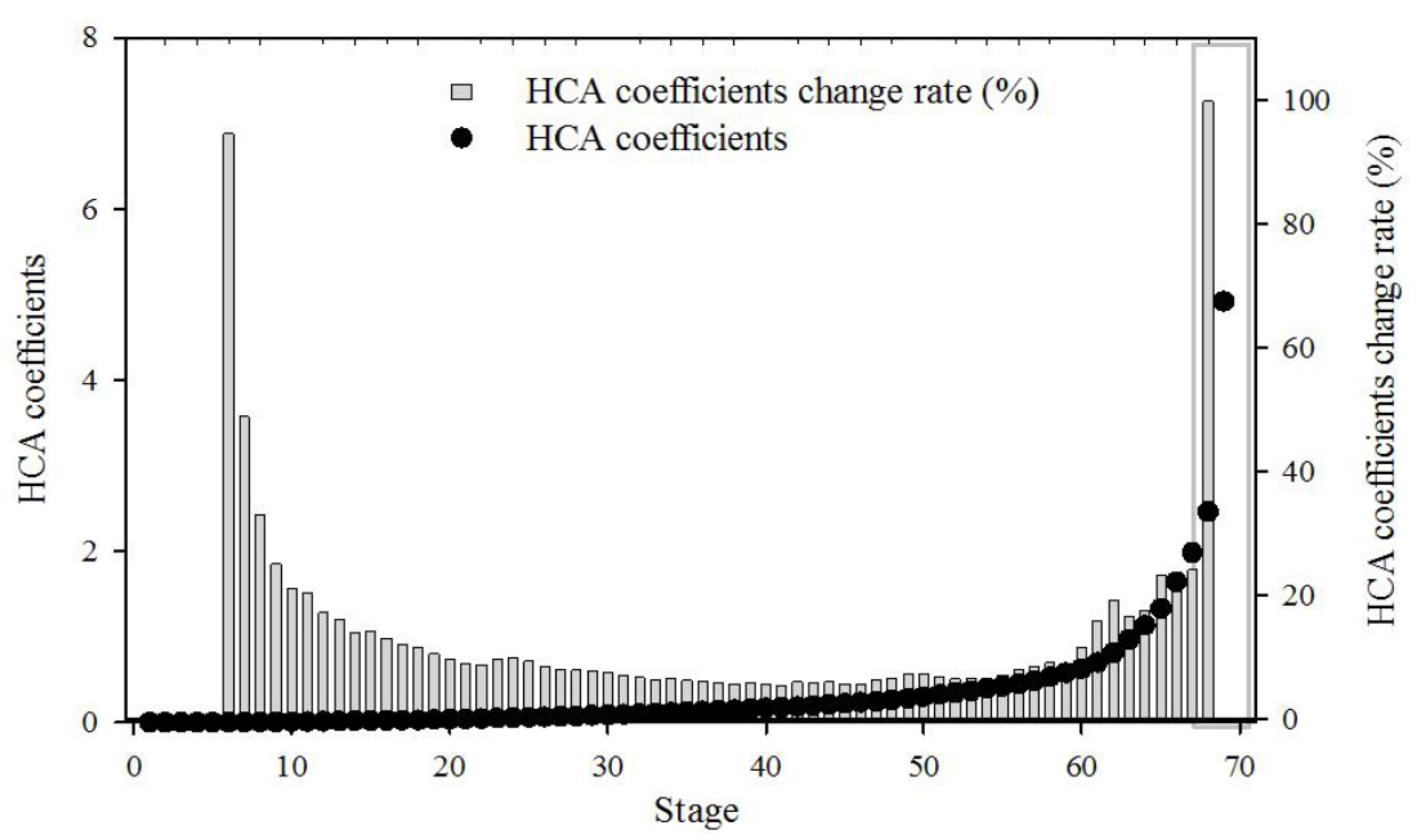
2.4.1. Hierarchical Cluster Analysis

Hierarchical cluster analysis (HCA) is based on a framework of hierarchy to divide or agglomerate the data from different layers repeatedly and generate a dendrogram. This study uses agglomerative hierarchical cluster analysis [56,57] by taking each of the 70 watersheds’ monthly NDVI time-series data as an individual cluster in the first stage and combining any two clusters identifying the clusters have the closest distance in between them. This procedure was carried out repeatedly until the number of clusters reaches an optimal number of this study. The optical number of this study remains unknown a priori and will be examined with further consideration of the spatial feature of vegetation and geographical environment in Taiwan. The present study applies the Ward linkage method considering the cluster with priority, which is based on the value of the total variance of the cluster to identify the distance between two clusters. When a group has the smallest variance, it is given priority to be grouped as a cluster. The earlier the stations to be grouped, the higher the similarity within the stations. The similarity measurement of Ward’s minimum variance method is based on squared Euclidean distance [58,59,60,61], the calculation is as follows:

$$d_{A,B}=n_A{\Vert \overline{x_A}-\stackrel{=}{x}\Vert }^2+n_B{\Vert \overline{x_B}-\stackrel{=}{x}\Vert }^2,$$

(1)

where d_A,B represents the distance between cluster A and cluster B, n_A and n_B represent the number of the points in cluster A and cluster B, respectively. ($\overline{x_A}$) and ($\overline{x_B}$) represent the central point of cluster A and cluster B, respectively, while $\stackrel{=}{x}$ represents the central point of the combined 2 clusters.

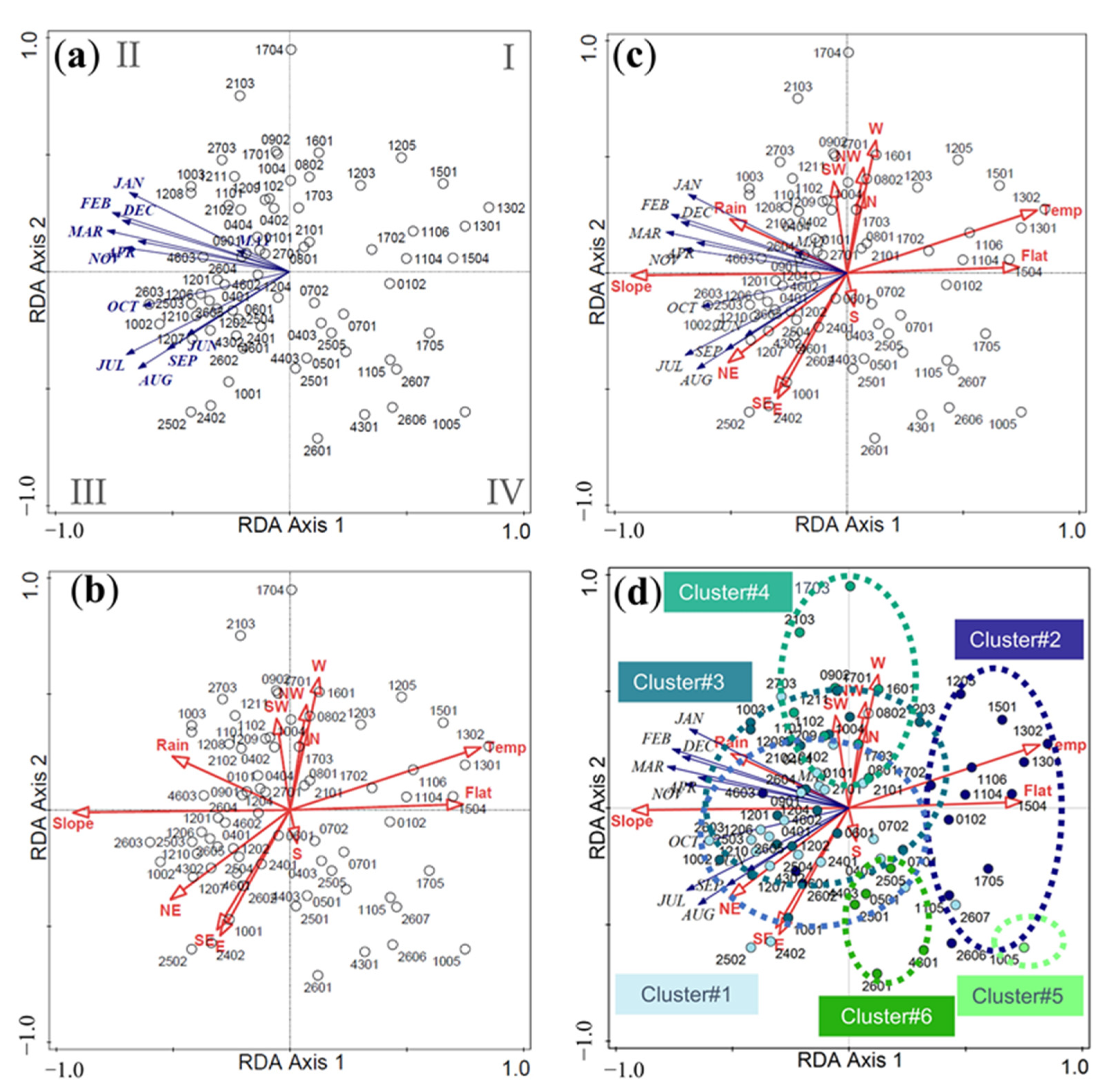
2.4.2. Redundancy Analysis

Redundancy analysis (RDA) is applied to explore the relationship between NDVI and environmental variables. Specifically, RDA also evaluates the explanatory power of each environmental variable, including climatic variables temperature and precipitation, and orographic variables aspect and slope, to the variations of NDVI across the entire study period. Rao [62] proposed the RDA in 1964, and the RDA was later explored again by Van DenWollenberg [63] in 1977. Redundancy is often identical to explained variance [64]. As an extension of multiple linear regression (MLR), RDA is allowed to have multiple explanatory variables (EVs) and a set of response variables (RVs) [65,66]. Furthermore, an RDA may also be considered an extension of principal component analysis (PCA) because the canonical ordination vectors are linear combinations of the RVs.

In general, the foundation of RDA is canonical multivariate analyses and assumes the relationship between variables is in a linear relationship [67]. The assumed linear relationship among the variables can be expressed by the Eigen analysis equation is as follows:

$$\left(S_{YX}{S}_{XX}^{-1}{S}_{YX}^{\prime }-{\lambda }_{k}I\right)u_k=0,$$

(2)

where S_YX is covariance matrix of variables and explained variables, S⁻¹_XX represents the inverse covariance matrix of normalized explained variables, I represents a unit matrix, λ_K is the Eigen value of axis k, and u_K denotes normalized canonical eigenvectors [65]. Detailed calculations and explanations can be found in Similauer and Leps [68].

In the present study, the NDVI values from each month represent the RVs, the environmental variables are the EVs, and the watersheds are the cases. The explanatory variables (EVs) refer to the environmental variables, including climatic variables, temperature and precipitation, and orographic variables aspect and slope. The aspects included flat aspect (Flat), north aspect (N), northeast aspect (NE), east aspect (E), southeast aspect (SE), south aspect (S), southwest aspect (SW), west aspect (W), and northwest aspect (NW). Consequently, a total of 12 EVs in the RDA analysis. This study verified the qualification of an RDA by applying a detrended correspondence analysis with a surveyed length of turnover units smaller than three. As the score scaling type was set with the focus on RV correlations, the output ordination diagrams of RDA can be interpreted from its biplot and triplot diagrams.

According to Similauer and Leps [68], the fundamental explanation rules for RDA biplots and triplots are summarized here. The symbols indicate cases, and the arrows indicate RVs and EVs. The concept of relative relationships has been the focus of all interpretations of ordination diagrams, for instance, the relative distances of symbols, the relative directions of arrows, and the relative ordering of projection points. Summarized interpretation guidelines are listed below:

• For the arrows, the pointed direction represents the maximum increase in the variable’s value across the diagram, and its length is proportional to the maximum rate of change.
• Project the case points perpendicular to the RV or EV arrow to obtain an approximate ordering of the value of one RV or EV across cases.
• Predict a case point projecting onto the origin of the coordinate system (perpendicular to an RV or EV arrow) to gain an average value of the corresponding variable. To obtain above and below-average values, the cases projecting further from zero in the direction of the arrow and opposite direction are predicted, respectively.
• The relative directions of arrows approximate the linear correlation coefficients among the variables. In other words, the value of an RV can be predicted to have a positive correlation with an EV value if that EV arrow points in an analogous direction to an RV arrow.
• The individual relationship of any two arrows is indicated by the cosine of the angles between the arrows. Any two variables will be predicted to have a weak correlation if the arrows intersect at a right angle (near to zero).

3. Results

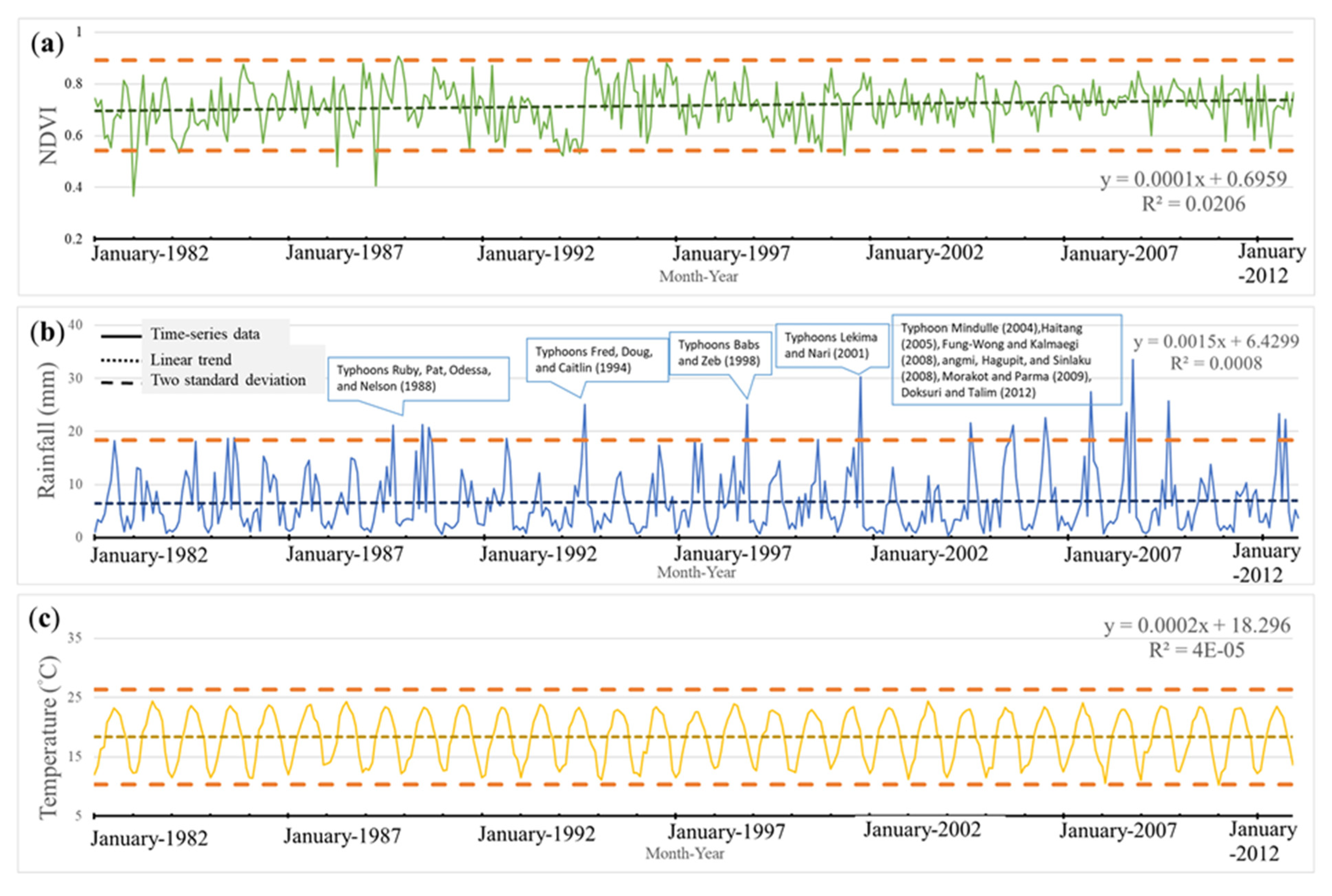
3.1. Time Series Data for NDVI, Rainfall, Temperature for Upstream Watershed

Figure A2 in Appendix B shows the 31-year average time series data of NDVI, rainfall, and temperature extracted from the selected 70 watersheds, having average values between 0.37‒0.97, 0.37‒33.49 mm, and 10.27‒24.36 °C, respectively. Additionally, linear trend analysis was employed with the data’s standard deviation calculated to assess the time series data.

As seen in Figure A2a, the NDVI values between 1993 and 1995 are lower, which may be attributed to the drought lasting for nine months in Taiwan during this period, as reported by Hsu et al. [69] and Tsai et al. [45]. As seen in the time series data for rainfall in Figure A2b, the higher values above two standard deviations were associated with past typhoon events. Apart from the drought between 1993 and 1995, another severe drought occurred in Taiwan during 2002 and 2004, as Hsu et al. [69] reported. Lower values of rainfall data, therefore, can also be seen during these periods. On the other hand, the result of rainfall peak values after 2004 occurred more frequently than before 2004. It will be worthy of discussing the relationship between this increased frequency and the effect of climate change. In addition, as shown in Figure A2c, the temporal variation of the temperature showed a steady undulation pattern of hot summer and cold winter. The oscillation of the value was approximately steady, and no noticeable change was observed during the drought and typhoon seasons.

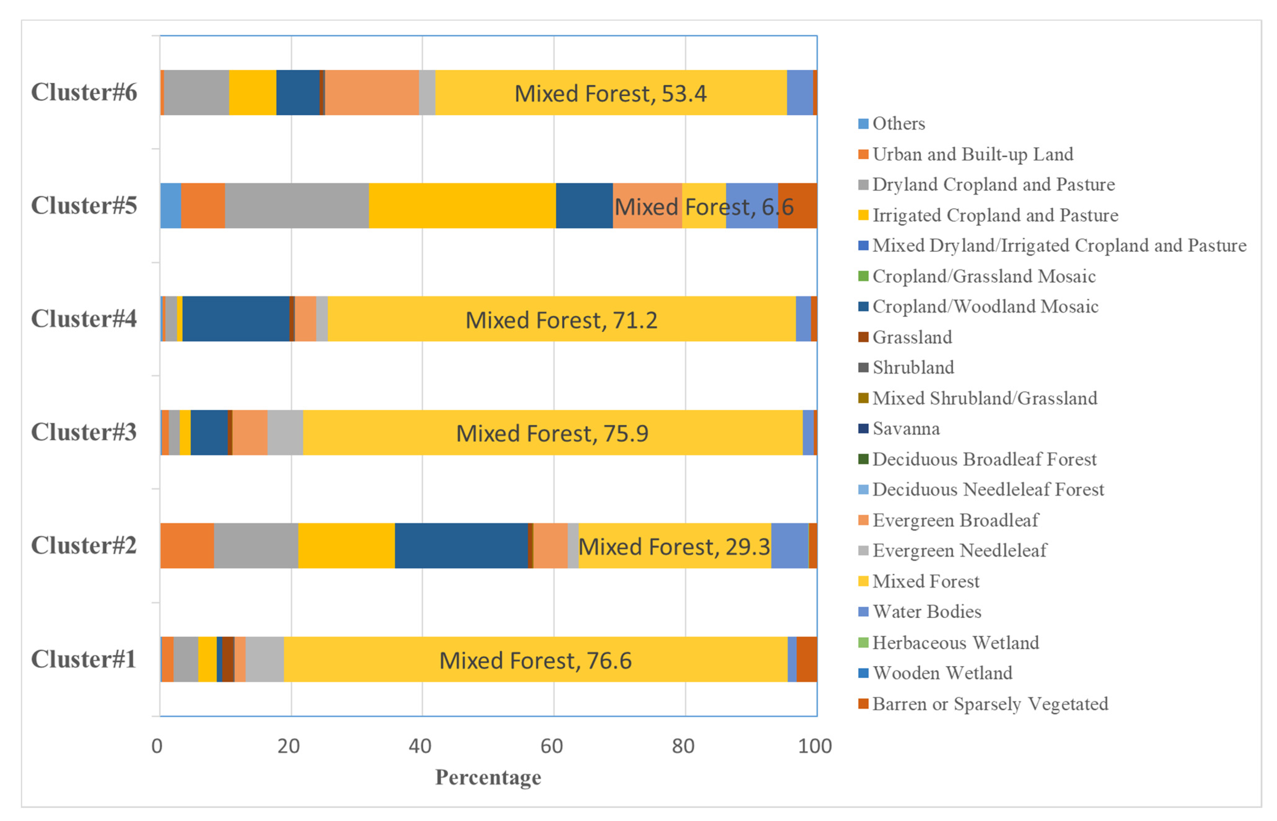
3.2. Cluster Analysis for Upstream Watershed NDVI

This study applied the agglomerative hierarchical cluster analysis (HCA) with Ward’s minimum variance method to judge the distance between clusters based on the monthly time series NDVI data. The highest variation ratio (99.7%) occurred at the 68th to the 69th stage from the preliminary result. According to the agglomeration definition of HCA, the optimal grouping stage is the 68th stage, and the optimal number of clusters is deduced to be two (see Figure A14). By considering the spatial feature of vegetation and geographical environment in Taiwan, however, the grouping stage was examined one by one for obtaining the optimal number of clusters. This is suggested to be six at the 64th stage, that this spatial pattern of vegetation clustering can reflect the spatial variation feature of vegetation in Taiwan.

The spatial distribution result of the cluster analysis is shown in Figure 2. The number of watersheds for each cluster is shown in

Table 1. Number of watersheds, average slope, and percentage of aspect for each cluster.

Cluster	Number of Watersheds	Slope (Degree)	Aspect (%)
			Flat	North	North East	East	South East	South	South West	West	North West
1	22	26.7	1	12	14	14	14	12	11	11	12
2	15	15.6	5	12	10	12	12	12	11	12	12
3	19	27.9	1	13	11	11	12	12	13	14	14
4	8	21.2	0	14	10	9	9	10	13	16	17
5	1	4.5	2	14	8	6	5	11	16	19	19
6	5	17.9	1	9	13	19	19	11	9	10	9

. Most of the watersheds in Cluster #1 are located at the east of the central mountain range. Cluster #2 is located at the western plains, and Cluster #3 is located at the higher elevation of the central mountain range. For Cluster #4, #5, and #6, most of the watersheds are located at southwest of Taiwan, the Dajia River, and east of Taiwan.

3.3. Identifying Important Driving Factors

The RDA analysis was applied to identify the environmental variables dominating the spatial characteristics of the NDVI signature of each cluster, including climatic variables temperature and precipitation, and orographic variables aspect and slope. Again, the monthly NDVI was the response variable (RVs), while the temperature, rainfall, slope, and aspect factors were the explanatory variables (EVs) in this analysis. Finally, the 70 selected watersheds were the cases.

As shown in

Table 2. Cumulative fraction of variation in individual monthly NDVI explained by the first, the first two, and all RDA axes.

Monthly NDVI	Axis 1 (%)	Axis 1 and 2 (%)	Total (%)
January	46.72	58.22	58.52
February	57.39	63.80	64.51
March	60.83	63.97	66.20
April	42.00	43.74	47.60
May	5.10	5.96	35.22
June	19.31	26.68	33.46
July	48.56	61.10	63.76
August	41.80	58.96	60.19
September	27.30	38.39	45.12
October	39.20	41.31	46.42
November	49.65	50.72	52.08
December	51.05	55.93	56.70
Average	40.74	47.40	52.48

, on average, the environmental EVs can explain approximately 52% of the monthly NDVI variance over the entire time series. In terms of temporal perspective, the NDVI signature of January to March, July to August, and November to December, revealed cumulative explained variance exceeded 50%. Additionally, the explanatory ability and the statistical significance level of the EVs for analyzing the variability of NDVI are shown in

Table 3. Explanatory ability and statistical significance level of variables to the NDVI variations. Significant variables are marked with stars.

Name of Variable	Explains (%)
Slope	35.2 ****
Temperature	27.8 ****
Flat	17.2 ****
North East	11.2 ****
Rain	10.6 ****
East	5.9 **
South East	5.7 **
West	5.2 **
North West	3.6 *
South West	2.7
North	2.5
South	0.3

**** p < 0.001; ** p < 0.05; * p < 0.10.

. The relationship between the NDVI value of watersheds and most of the EVs was significantly related at different significance levels. According to the result of statistical significance level, nine important driving factors which relate to the watershed are slope, temperature, flat aspect (Flat), northeast aspect (NE), rainfall (Rain), east aspect (E), southeast aspect (SE), west aspect (W), and northwest aspect (NW). Among these factors, the slope has the highest value of explanatory ability (35.2%, p < 0.001), as shown in Table 3.

The RDA results of the biplot showing NDVI and watersheds are shown in the biplot of Figure 3a. The quadrants of the biplot are numbered in an anti-clockwise direction, showing Quadrant I on the upper-right corner of the plot. Based on the principles of RDA, the length of the NDVI arrows (RVs, shown in blue arrows) shows how much the NDVI variability of each month can be explained by all explanatory variables (EVs, shown in red arrows). Additionally, an approximate ordering of the NDVI value (RV) across watersheds can be discerned by projecting the watershed point perpendicular to the RV arrow to obtain.

As a result, the length of the arrows for the period of January to March, July to August, and November to December is relatively longer than other periods. The results indicate that the NDVI variability can be explained by the RVs efficiently. The results also respond to the cumulative variation in individual monthly NDVI explained by RDA axes shown in Table 2. The cumulative explanatory variance of those months exceeds 50%.

Furthermore, the included angle between two arrows indicates the relevance of the arrows, where the smaller the included angle, the higher the correlation is. As seen in the biplot of Figure 3a, the angles between each month’s NDVI were less than 90 degrees, indicating a positive correlation (95% CI) between each month’s NDVI. Moreover, the arrows of June to September in Quadrant III and the arrows of November to next May in Quadrant II were closer to each other. It may imply a changing seasonality pattern or seasonality diminishment revealing climate change influences.

Figure 3b shows the relationships between the watersheds, the EVs, and the explanatory ability of each EV as a biplot. For example, the angle between temperature (Temp) in Quadrant 1 and slope (Slope) in Quadrant III was larger than 90 degrees, indicating a negative correlation between these two variables. In other words, the higher the slope, the lower the temperature, reflecting the lapse rate common sense. Likewise, the angle between rain (Rain) and slope (Slope) is smaller than 90 degrees, representing a positive correlation between rain and slope. Thus, the higher the slope, the more considerable amount of rain that occurs.

The length of the arrow in the triplot Figure 3c indicates the explanatory ability of the variable, in which the longer the arrow, the better the explanatory ability is. Figure 3c and Table 3 show that the slope (Slope) variable has the highest explanatory ability. The temperature (Temp) and the flat (Flat) rank the second and the third one of the explanatory ability. Additionally, the rain, NE, E, SE, W, and NW variables have different explanatory abilities for NDVI.

The correlation between the RVs (NDVI) and EVs (the environmental variables) is shown in Figure 3c. The direction of the arrows and the included cosine of the angles between any two arrows indicate their correlation. The arrows of the slope, rain, NE, E, and SE (see Quadrant II and III) have the same direction as the arrows of NDVI for every month; thus, these EVs correlate positively with NDVI. Furthermore, the included angles for the NDVI values from November to next March are similar to the included angle of rain in Quadrant II, showing that the NDVI values positively correlate with rain from November to next March. On the other hand, the direction of the arrows of Temp and Flat is different from the arrows of NDVI, thus leading to Temp and Flat having a negative correlation with NDVI. With the higher accessibility of flat land, it is reasonable to have higher accessibility, thus a higher level of human settlements. Accordingly, the decrease in NDVI can be attributed to excessive human activity, such as urban development in the flat area.

Figure 3d shows the combined RDA and HCA results. The spatial distribution of the watersheds HCA results demonstrate the spatial feature of the clusters. Cluster #1 (circled in light blue) is located at the middle and slightly left from the middle of the figure, as most of the watersheds appear in Quadrant III. The spatial presence with RVs and EVs indicates that the watersheds in Cluster #1 have higher monthly NDVI value, higher average slope value, and more rainfall. The watersheds of Cluster #2 (circled in dark blue) are located at Quadrant I and IV, indicating the watersheds of this cluster having lower NDVI value, less rainfall, lower average slope, higher temperature, and have more flat areas. For Cluster #3 (circle in indigo), the watersheds are located next to Cluster #1, demonstrating that both clusters have similar features.

The watersheds of Cluster #4 (circled in dark green) are located at Quadrant I and II in Figure 3d. It shows that the W and N aspects are the main aspect, and the value of the average slope is close to the mean value of the selected 70 watersheds. Cluster #5 (circled in light green) is located at the lower right of Quadrant IV in the figure, indicating the watersheds’ high temperature and flat slope features. Finally, Cluster #6 (circled in green) is located at the lower side of Quadrant IV close to Quadrant III in the figure. Again, it demonstrates temperature values, and the slope of the watersheds in this cluster is close to the mean value of the selected 70 watersheds.

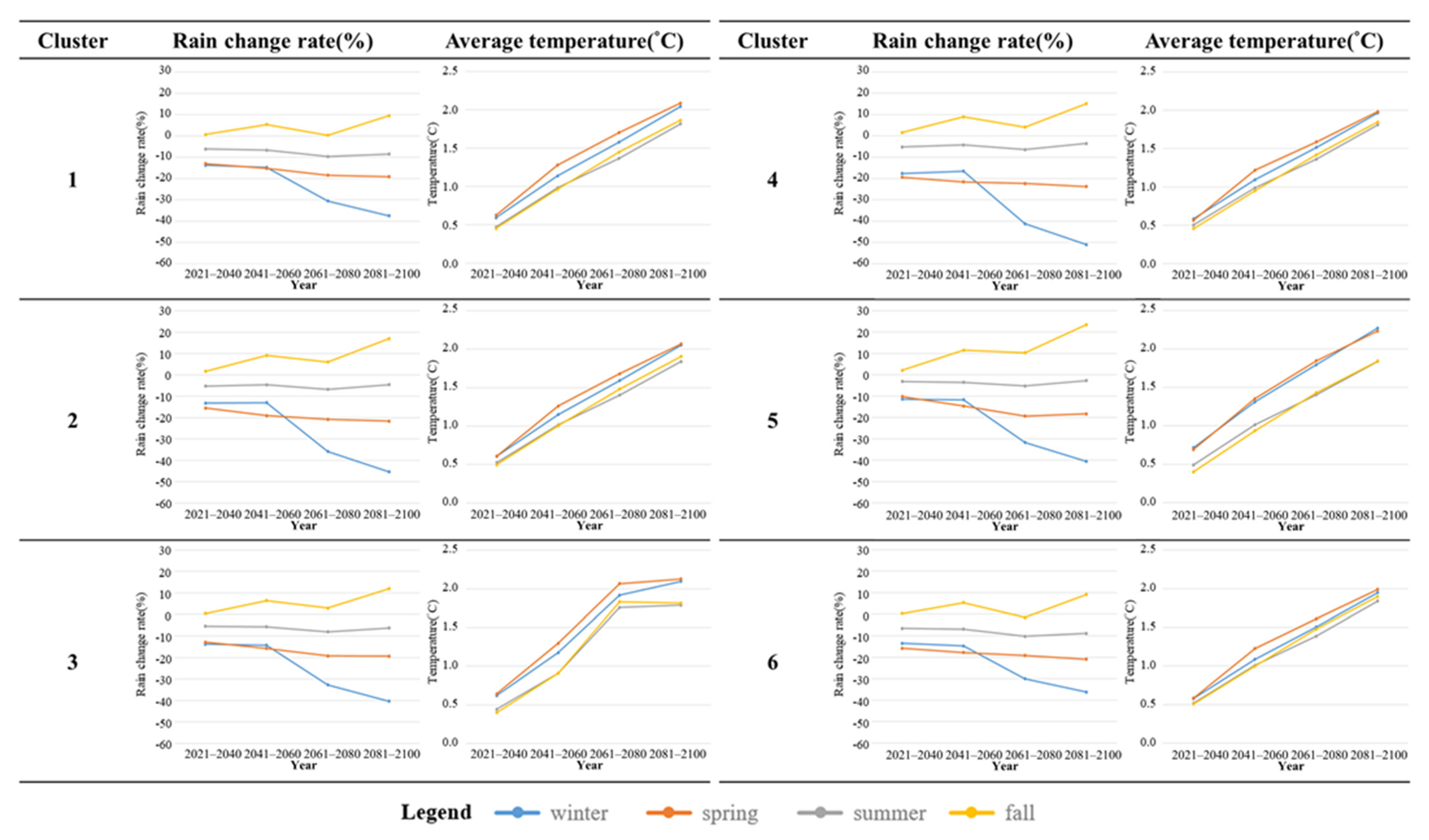
3.4. Climate Change Scenarios for Each Cluster

The temporal variations of the rain change rate and temperature data of watershed clusters under climate change scenarios are discussed in this section. The climate change scenarios are referred to the results indicated in IPCC’s fifth assessment report (AR5). The monthly values of simulation from the scenarios are averaged and discussed in four seasons, including winter (from December to next February), spring(from March to May), summer(from June to August), and fall (from September to November).

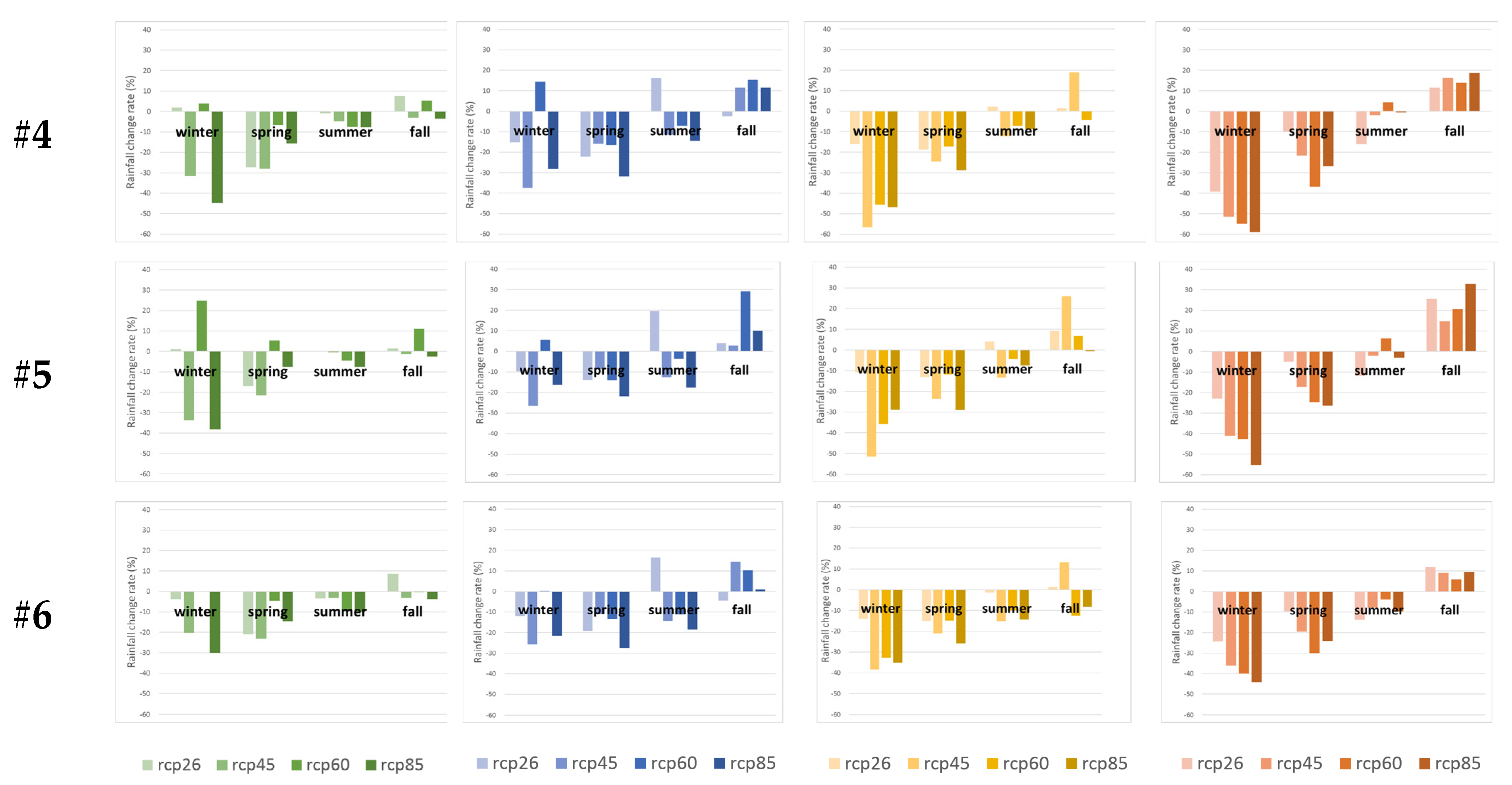
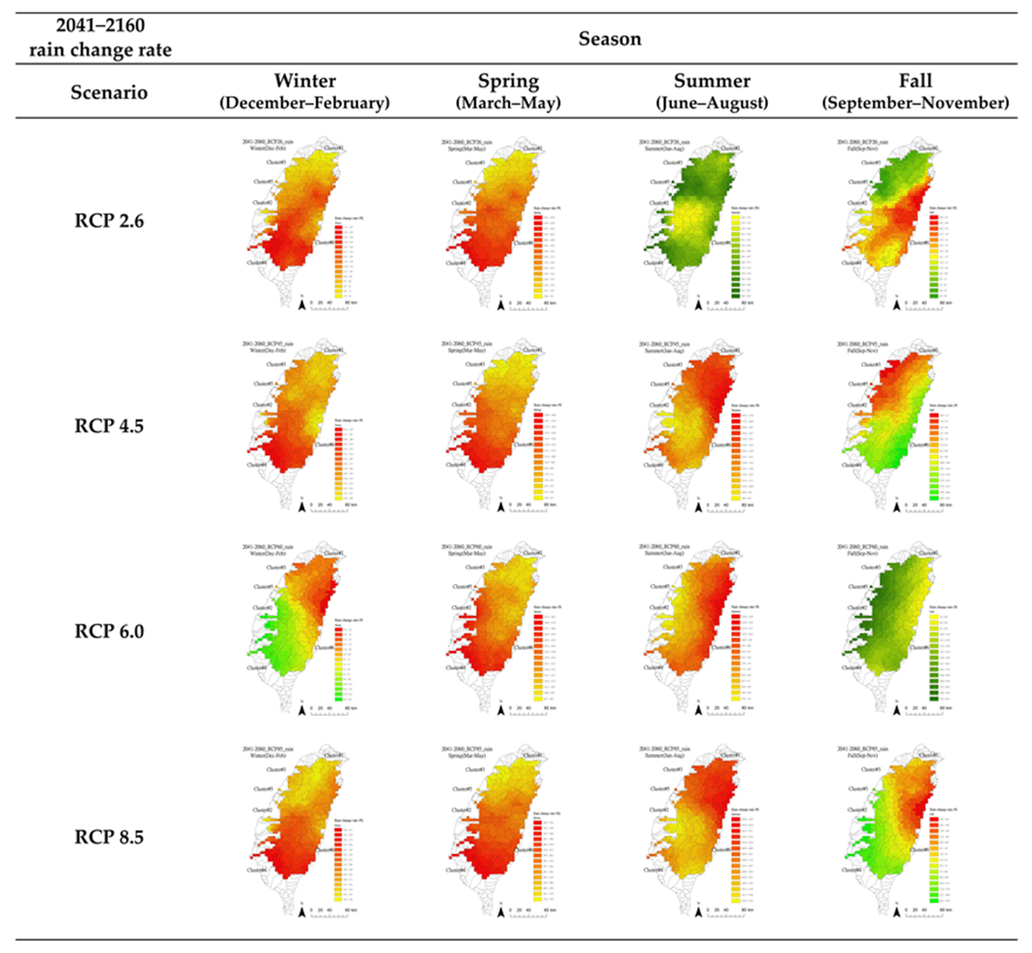
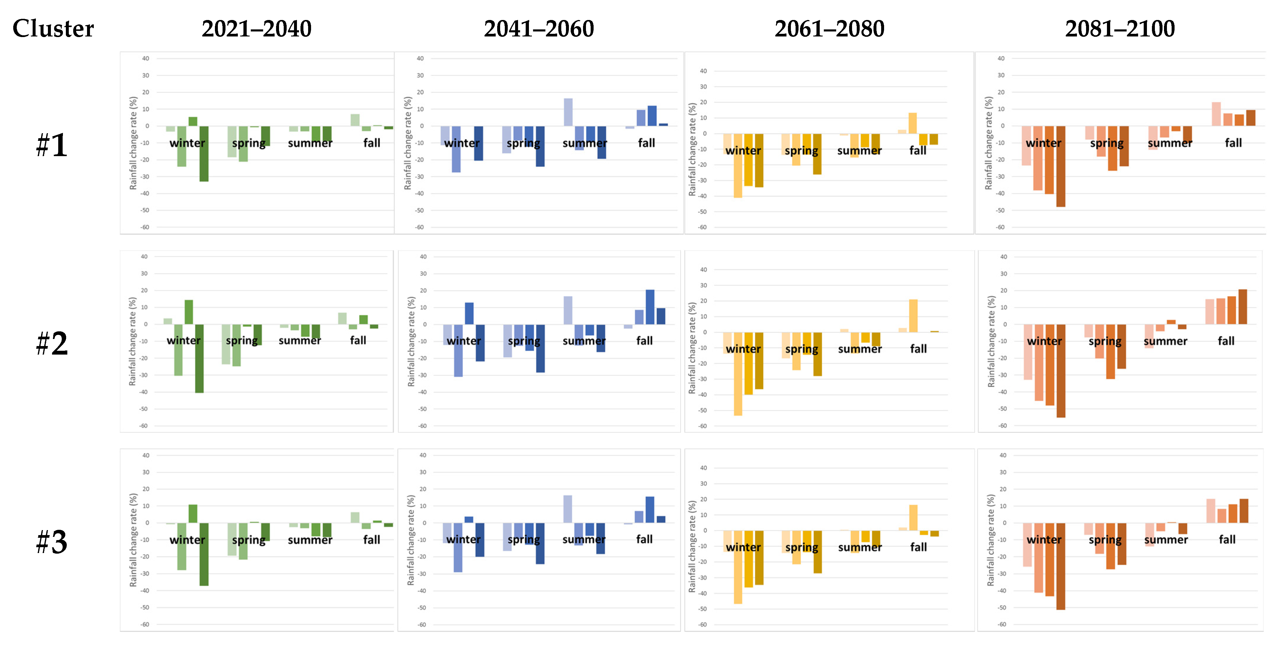
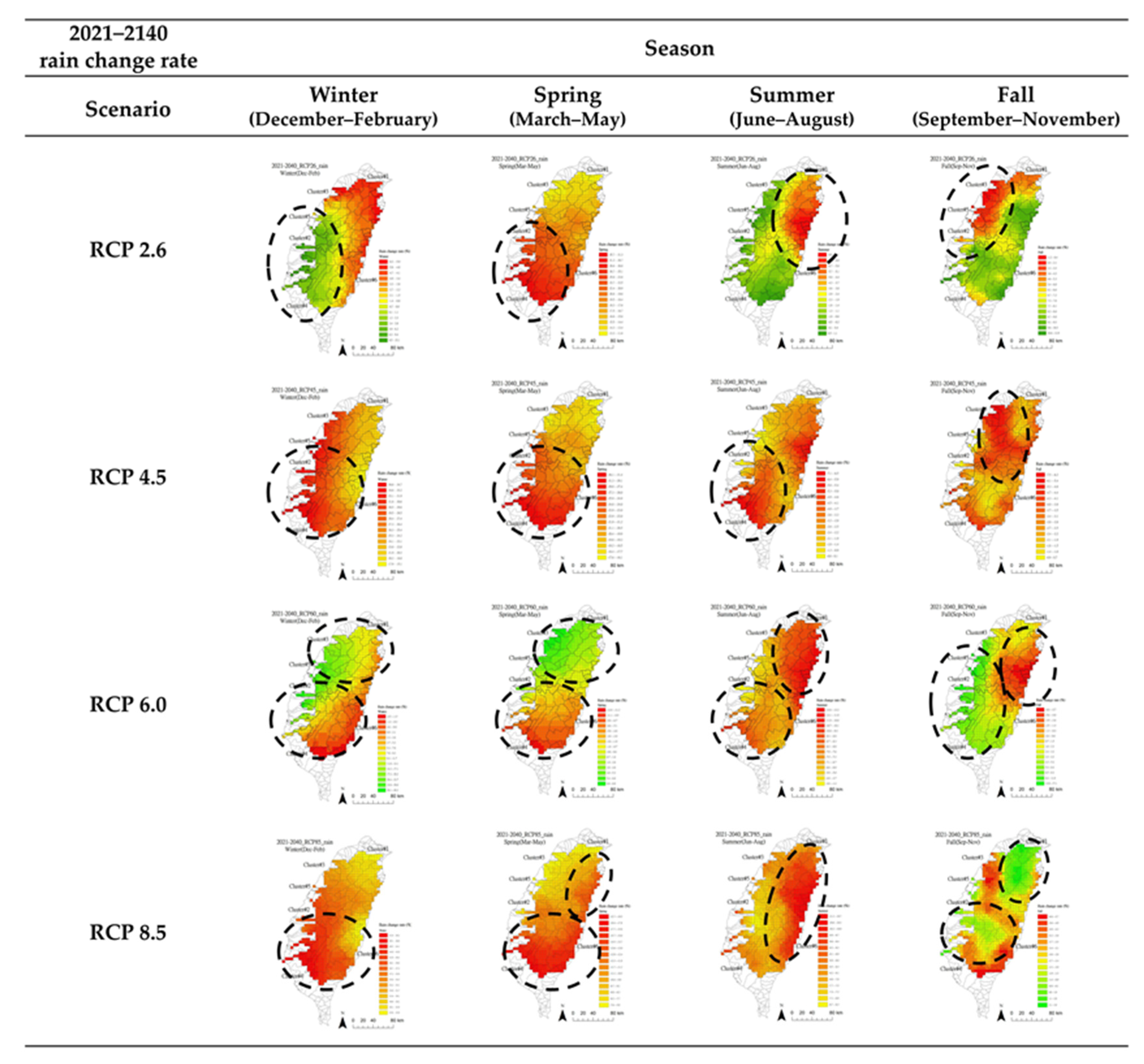
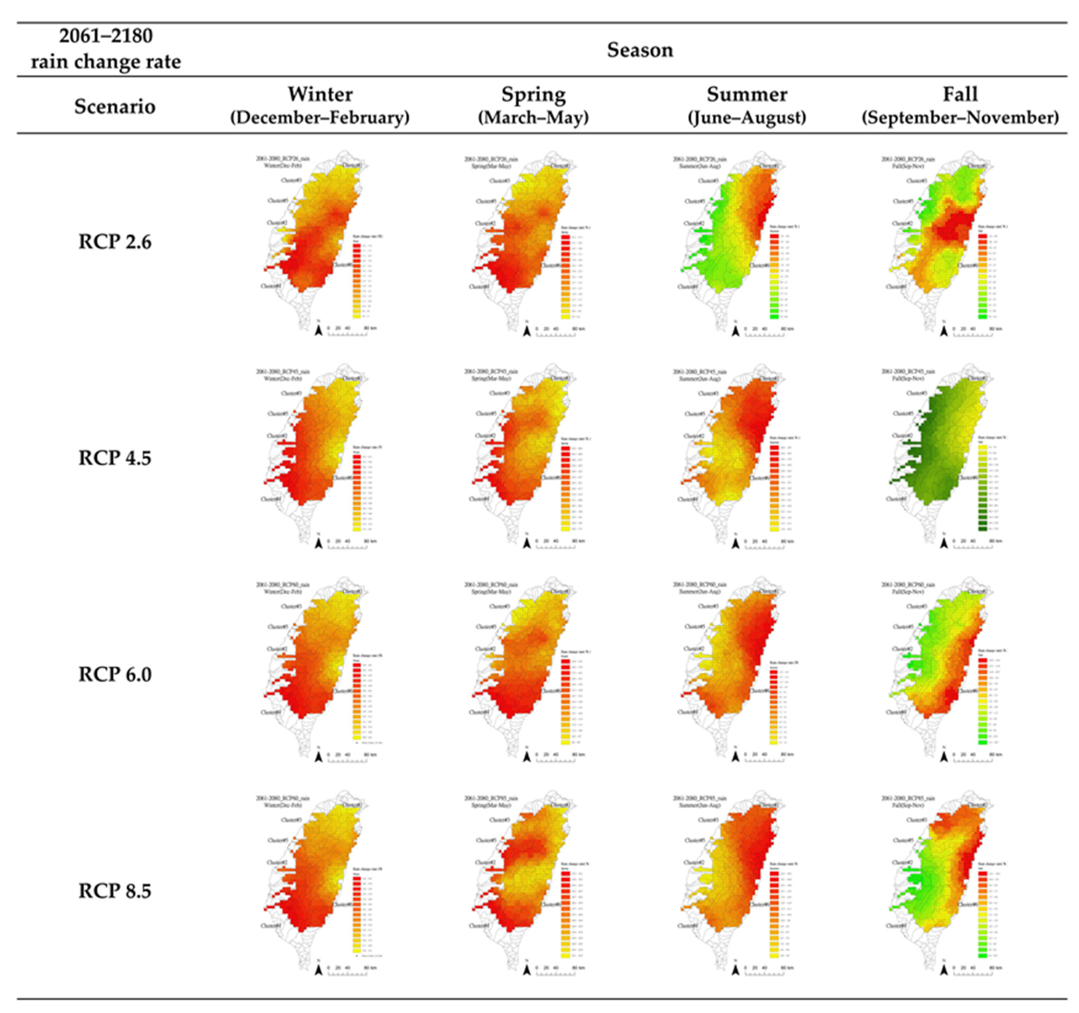
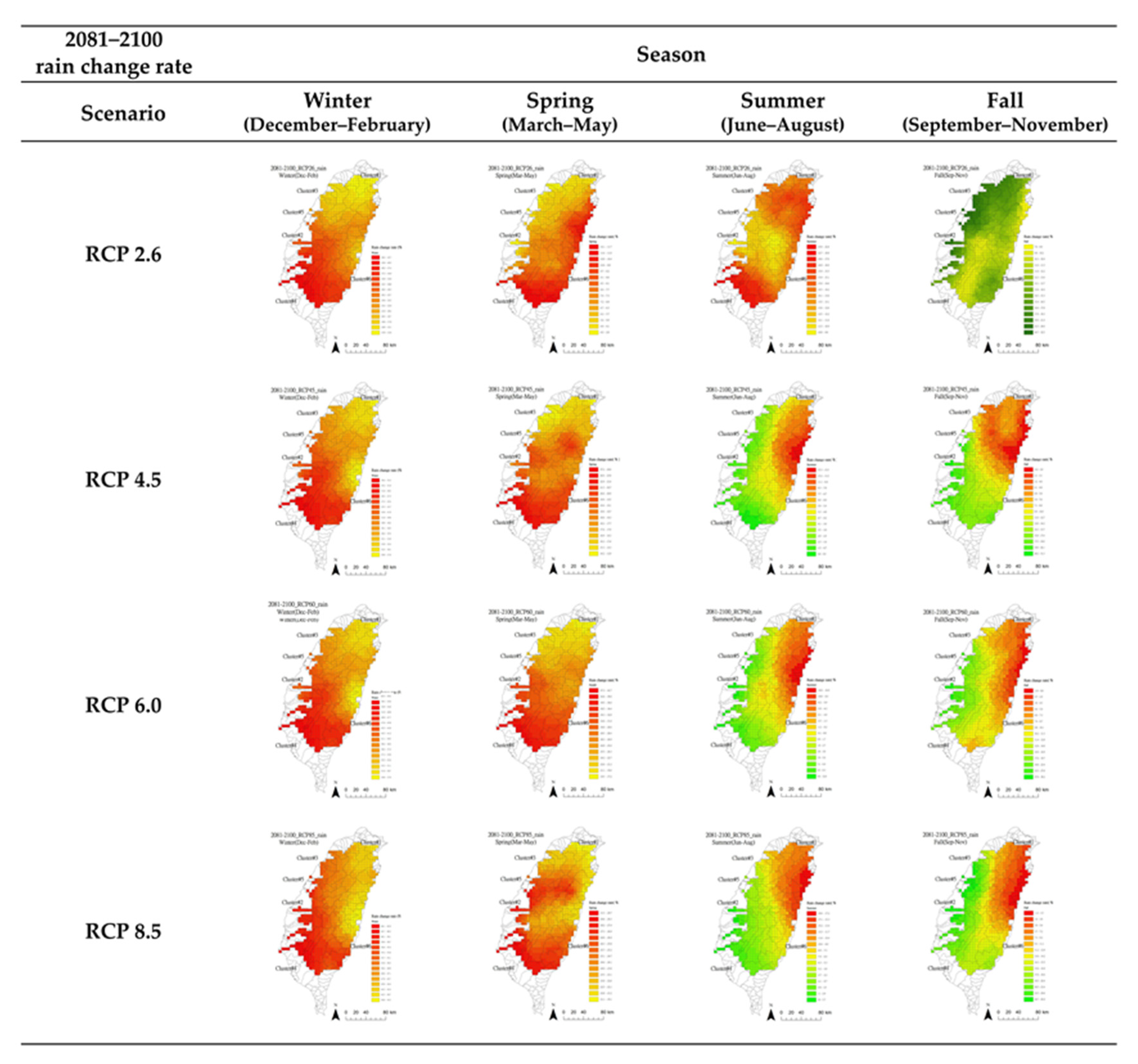
3.4.1. Rainfall Change Rate for Each Cluster

Figure A3 in the Appendix B illustrates each cluster’s seasonal rainfall change rate under climate change scenarios from 2021 to 2100. Generally, the rainfall change rates are negative in winter, spring, and summer but positive in fall. The value of the rates increases as the RCP level increases.

In the near future period of 2021 to 2040, rainfall change rates are predicted to decrease approximately 40% in winter in Clusters #2, #4, and #5 in the worst scenario RCP 8.5. However, scenario RCP 6.0 shows a 24% increased rainfall prediction in winter in Cluster #5. From 2041 to 2060, negative change rates are observed in winter, spring, and summer, except under scenario RCP 2.6 in summer. In winter, the largest decrease is observed in Cluster #4, around 37%, while the largest increase was observed in the fall in Cluster #5 at 29%. The decreased rainfall pattern in winter, spring, and summer with an increase in fall is evident in 2061–2080 and 2081–2100. The most significant decrease in winter rainfall occurs in Cluster #4 by 56% (in RCP 4.5) and 58% (in RCP 8.5) in 2061–2080 and 2081–2100, respectively.

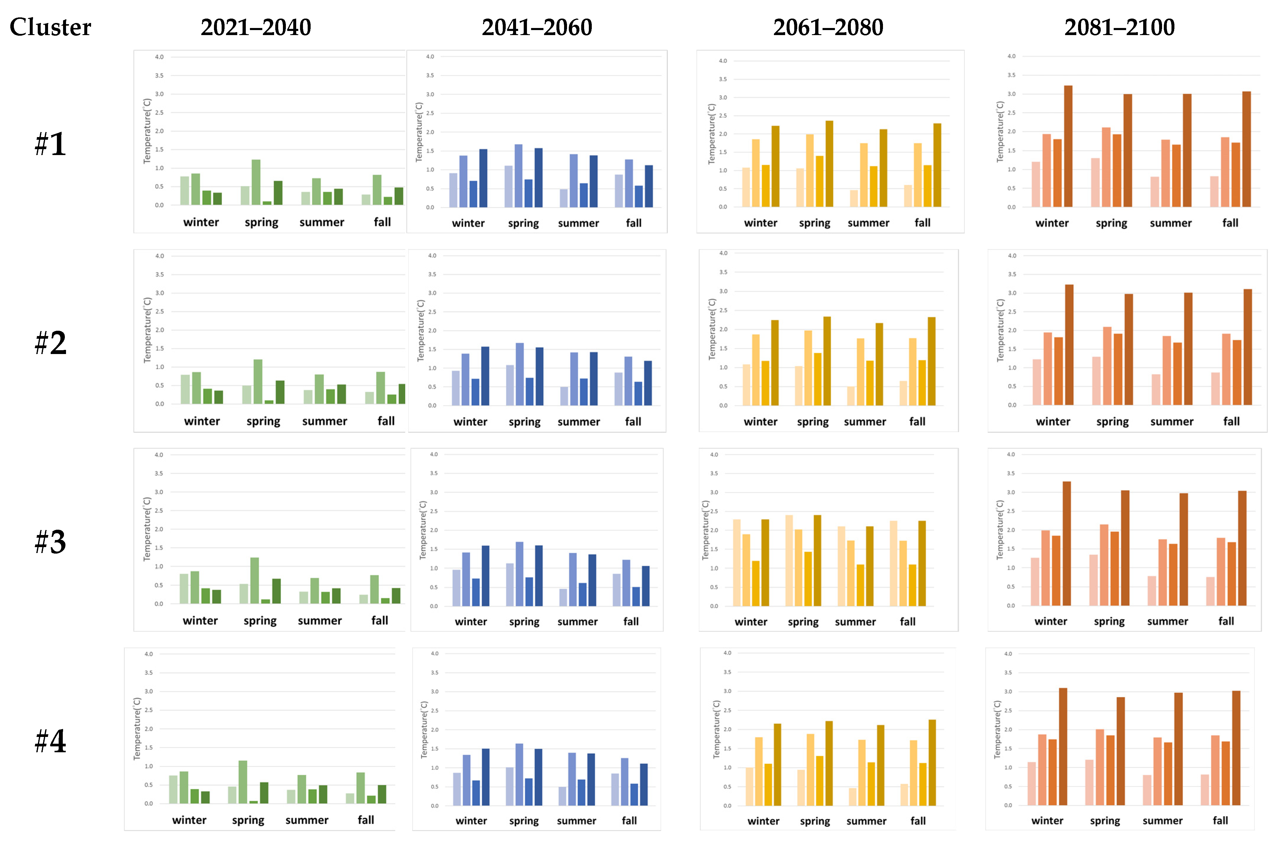
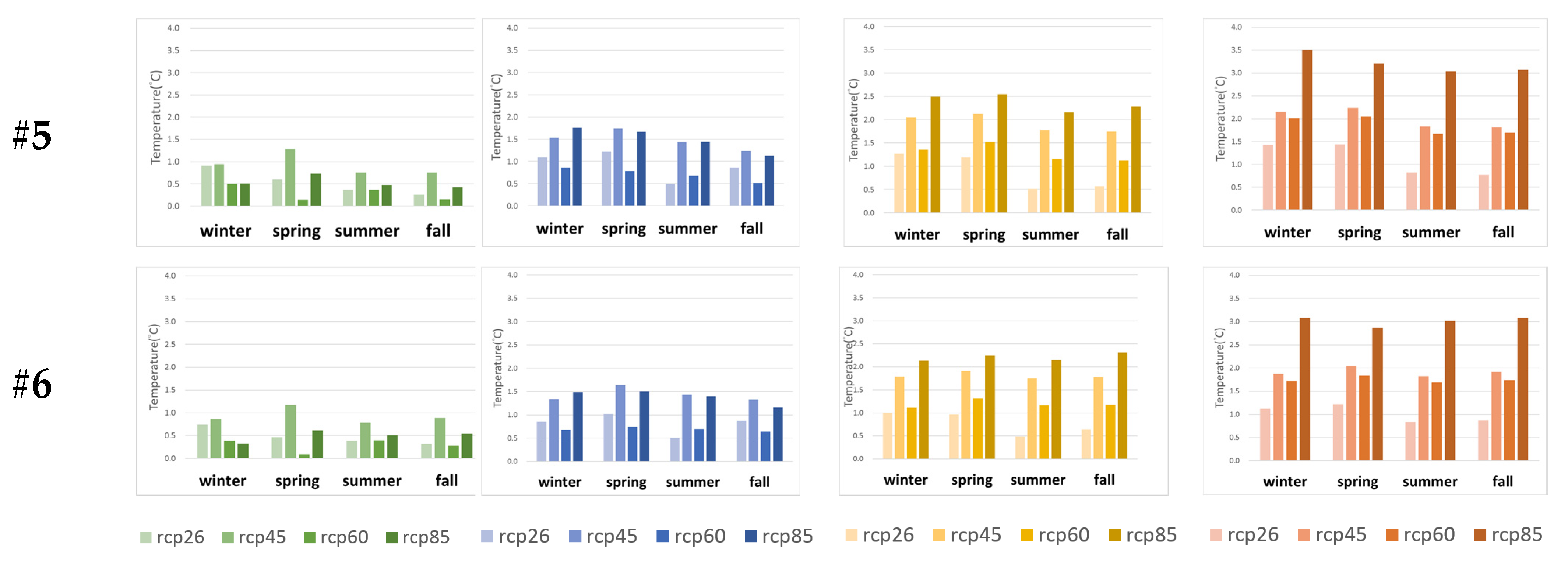
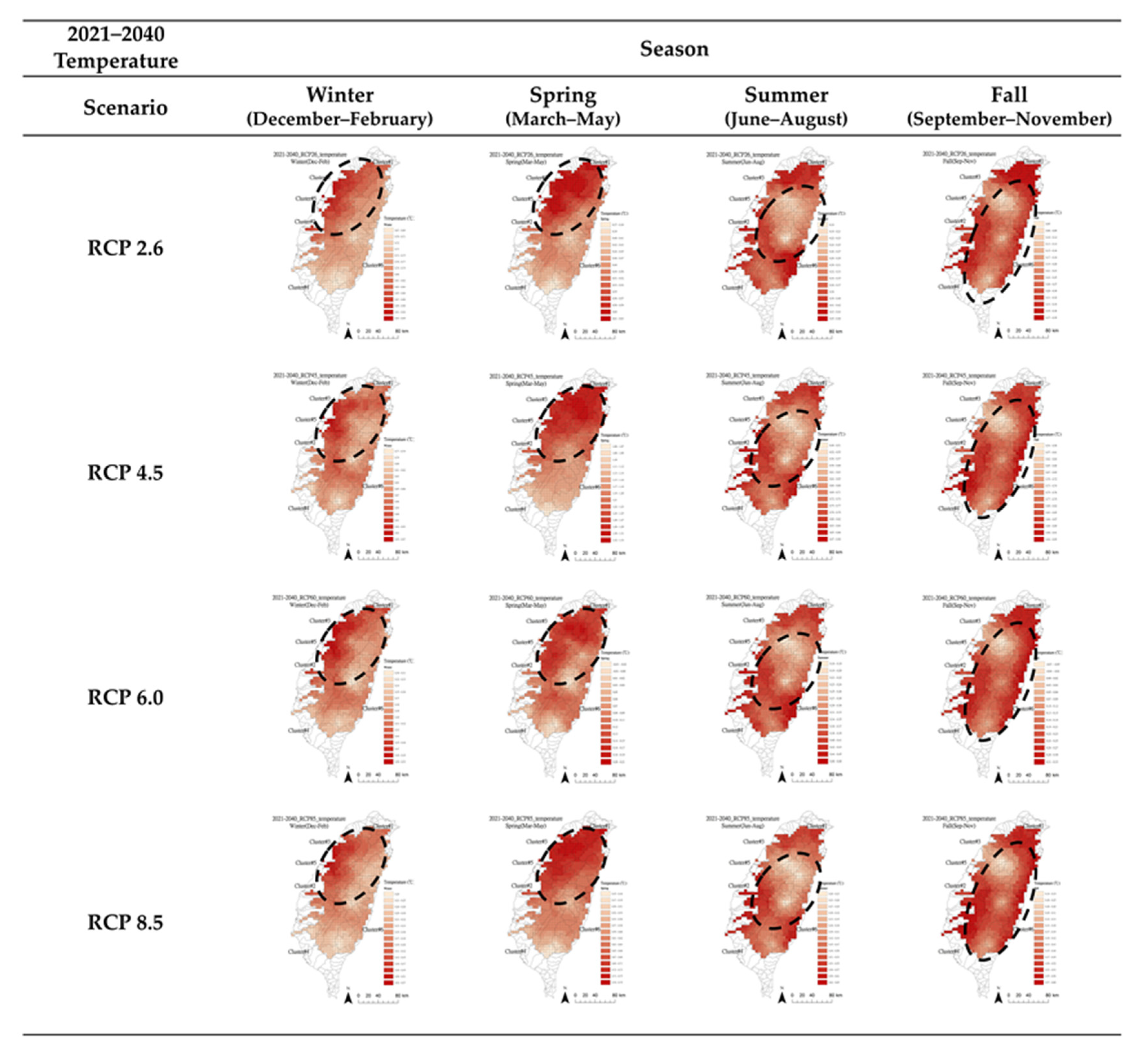
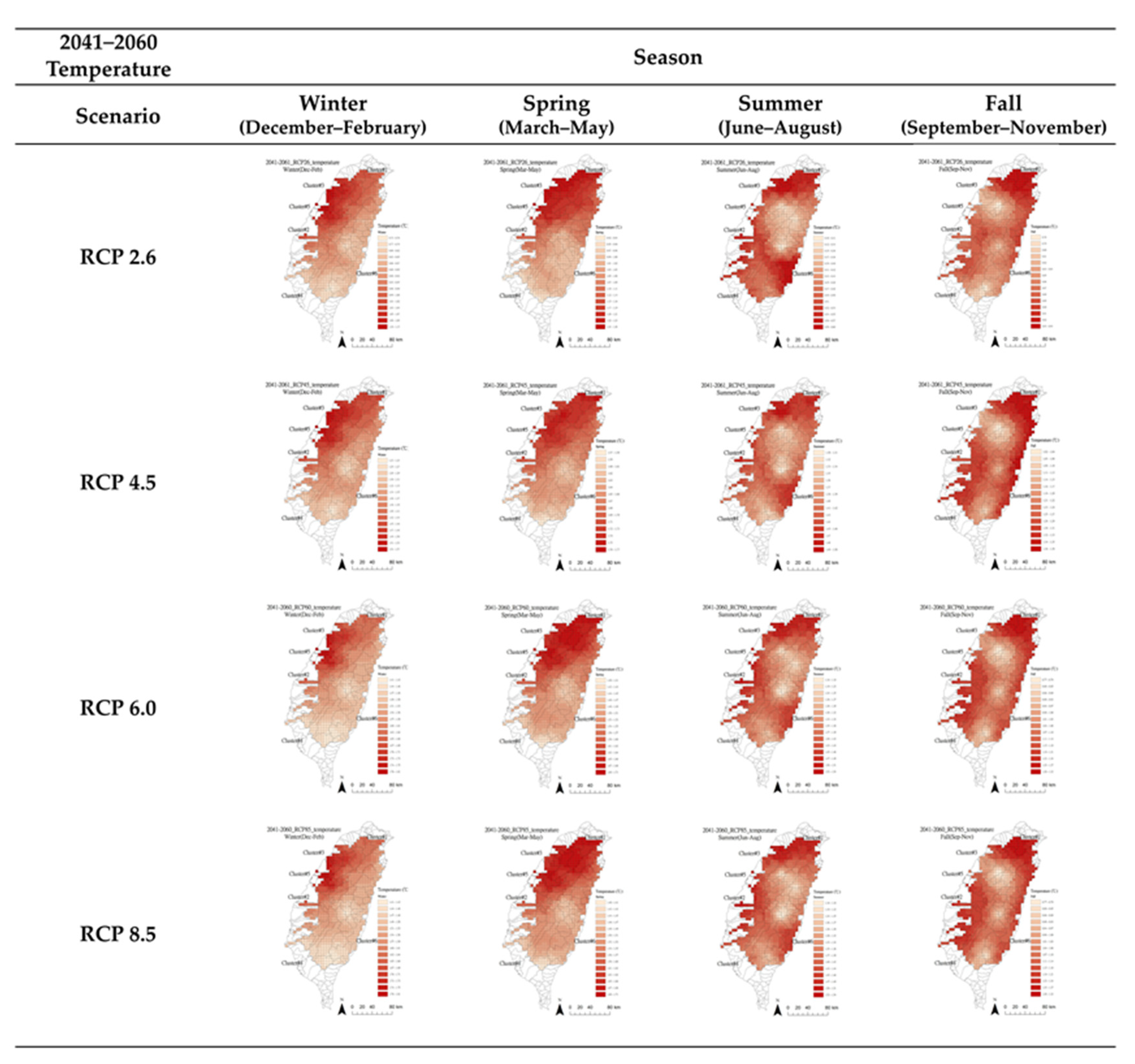
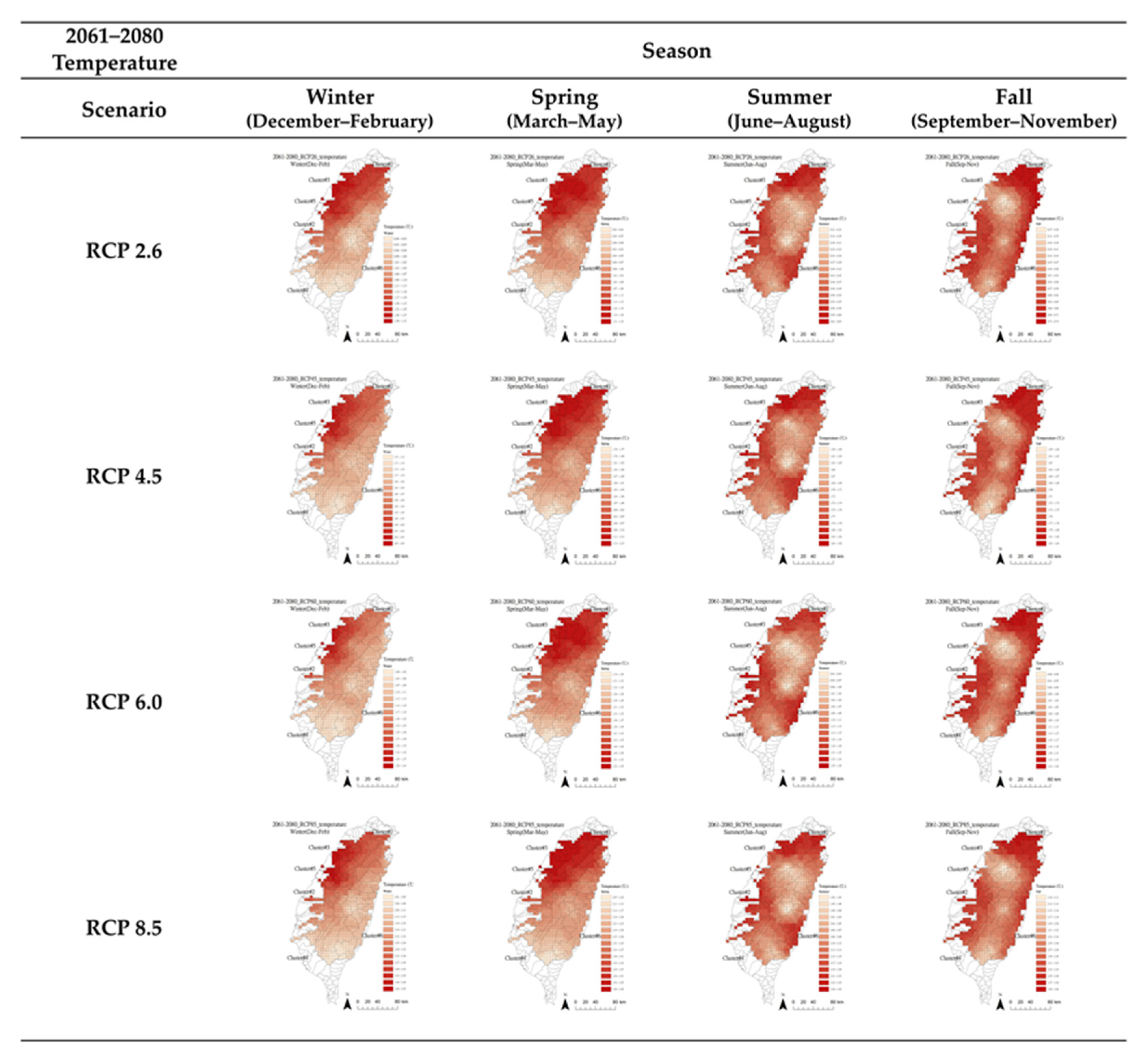
3.4.2. Temperature Change for Each Cluster

Figure A4 in the Appendix B shows each cluster’s seasonal temperature changes under climate change scenarios from 2021 to 2100. In general, the temperature increase for all clusters in all scenarios from 2021 to 2100, showing the smallest increase of 0.1 °C under the RCP 6.0 scenario and the largest increase of 3.5 °C under the RCP 8.5 scenario.

From 2021 to 2040 and from 2041 to 2060, the largest temperature increase is observed in spring, by approximately 1.2 °C and 1.5 °C in all clusters in the RCP 4.5 scenario. In 2061–2080, Cluster #3 displays a unique pattern by the most significant temperature increase in spring by 2.4 °C under the RCP 2.6 and RCP 8.5 scenarios. Other clusters show a similar pattern with the smallest increase in summer (0.4–0.5 °C, in the RCP2.6 scenario) and the largest increase in spring (2.4–2.5 °C, in the RCP8.5 scenario). Finally, from 2081 to the end of the century, the largest increase by 3.5 °C in Cluster #5 is expected under the RCP 8.5 scenario.

3.4.3. Temporal Variation of Rain Change Rate and Temperature Data

The average values of the rain change rate and temperature data for four scenarios (RCP2.6, RCP4.5, RCP6.0, and RCP8.5) during 2021–2040, 2041–2060, 2061–2080, and 2081–2100 were calculated and presented in Figure 4 to enhance comprehension understanding of climate change from near to distant future in each cluster for different seasons. Figure 4 shows that during fall, the rainfall has an approximately 10% of increment. In particular, during 2081–2100, the fourth and fifth clusters’ rainfall was predicted to have an increment higher than 10%. On the other hand, the rain change rate shows negative during winter, spring, and summer, which means the rainfall decreases during these seasons. Particularly in spring has a higher rain change rate than in winter; additionally, there is an evident decrement during 2061–2080 and 2081–2100 in winter.

It is shown that the variation of temperature has a general trend of increase, and the increased range is around 0.5 °C to 2 °C. The increment of the temperature during spring and winter is higher than that during summer and fall. Except for the third cluster’s temperature reached the peak value from 2061 to 2080, the trend continues to stay flat and mitigate from 2080 to 2100; the rest of the clusters have an increase in temperature from 2021 to 2100.

3.5. Potential Debris Streams and Affected Areas

Table 4. The number of potential debris streams and affected areas in each cluster.

Cluster	(A) Number of Sites of Potential Debris Stream Affected Area	Ratio of (A) to the Total Number of Sites	(B) Number of Potential Debris Streams	Ratio of (B) to the Total Number of Streams
1	370	19.9	337	19.5
2	237	12.7	199	11.5
3	614	33.0	531	30.8
4	219	11.8	155	9.0
5	4	0.2	6	0.3
6	166	8.9	139	8.1
Sum	1610	86.4	1367	79.2
Total number of sites/streams	1863		1726

and Figure 5 show the spatial relationship between watershed clusters with potential debris streams and affected areas. In particular, the potential debris streams and affected areas in Cluster #1 are distributed in the northern part, approximately 20% of the ratio to the total number of that in Taiwan. The potential debris streams and affected area in Cluster #2 is limited to around 12.7% of Taiwan’s total sites. Most of the potential debris streams locate in the eastern part and close to the central mountain range.

Cluster #3 has the most magnified number of potential debris streams, around 30% of Taiwan’s total potential debris streams. Additionally, Cluster #3 has the highest ratio of 33% of the number of potential debris streams affected areas, 614. On the other hand, Cluster #4 has around 9–12% of potential debris streams and affected areas. Furthermore, there is less than 1% potential debris streams and the affected area in Cluster #5 with only six potential debris streams. Finally, Cluster #6 has around 9% of the potential debris streams affected areas and 139 potential debris streams.

Therefore, in each cluster’s ratio, the potential debris stream-affected areas of Clusters #3 and #1 have higher ratios, which are 33% and 19.9%, respectively. Overall, the upstream watersheds contain 86.4% of the total potential debris stream-affected area and 79.2% of the debris streams in Taiwan.

4. Discussion

The present study has identified six clusters of the upstream watersheds in Taiwan based on their long-term NDVI signatures. Additionally, the NDVI signatures reveal a changing seasonality pattern or diminishment based on the RDA results, implying potential climate change influences. Moreover, increasing temperature and rainfall variations are expected for upstream watersheds under the climate change scenarios. Therefore, the seasonality diminishment, increasing temperature, and rainfall variations are discussed below, followed by climate change adaptation and mitigation strategies for each cluster.

Seasonality diminishment is observed in many northern high latitude areas in the world. For instance, Xu et al. [70] reported that the temperature difference between summer and winter temperatures is diminishing over time in the Arctic (boreal) region. As the diminishment trends continued, vegetation seasonality could be modified due to the alterations of termination and performance of vegetation photosynthetic activity tied to temperatures. Hence, Bhatt et al. [71] further investigated the changing seasonality of panarctic tundra vegetation related to climatic variables. The authors also used the same dataset as the present study, GIMMS NDVI3g, to study the vegetation response to temperature from 1982 to 2015. In addition, they obtained sea ice data together to demonstrate the influence of change temperature. Based on their results, they have found a significant NDVI decline in spring. Many possible drivers explained the early growing season NDVI decline, such as increased standing water, delayed spring snowmelt, winter thaw events, and early snowmelt followed by freezing temperatures. In the present study, a possible seasonality changing pattern has been observed based on the RDA results. The upstream watersheds contain high mountains with vegetation species sensitive to changing temperature influences, raising precautions for climate adaptation preparations.

Additionally, the predicted temperature change across all clusters is in good agreement with many scholars. Hsu and Chen [72] examined Taiwan’s climate change characteristics over the past 100 years. They concluded that the rainfall tends to increase in northern Taiwan and decrease in southern Taiwan with a complicated spatial pattern. The author also found the changes in rainfall occur mainly in either the dry or rainy season, resulting in an enhanced seasonal cycle. Finally, they observed the island-wide warming trend at the rate of 1.0–1.4 °C/100 years. Lin et al. [73] examined the climate variability of heatwaves according to air temperature and relative humidity to determine trends of variation and stress threshold in three major cities of Taiwan, Taipei, Taichung, and Kaohsiung. Based on the data from 2003 to 2012, they simulated future warming scenarios for 2075 to 2099. They concluded the heatwave stress would either exceed or approach the danger level by the end of this century.

Moreover, for Central Taiwan, Shou and Yang [32] performed a predictive analysis of landslide susceptibility under climate change. They have found that the mid-to-upstream and upstream areas of the Chingshui river were highly susceptible to landslides. In addition to landslides, the midstream and the upstream landslides may generate debris flow hazards during a heavy rainfall event. For Northern Taiwan, Chen et al. [74] assess future landslide characteristics using ensemble climate change scenarios for two catchments in northern Taiwan. Their ensemble results indicated that the landslide magnitude triggered by medium- and high-level typhoons would increase by 24–29% and 125–200% under climate change. Finally, for Southern Taiwan, Shou et al. [35] employed rainfall frequency analysis and the atmospheric general circulation model downscaling estimation to understand the temporal precipitation trends, distributions, and intensities in the Ai-Liao watershed located in southern Taiwan. The results reveal a highly susceptible landslide chance in the mid-upstream and upstream areas of the Ai-Liao watershed.

Based on the six clusters analyzed in Section 3 and future climate change scenarios, this study proposes adaptation strategies for each cluster. Most of the watersheds in Cluster #1 are located at the east of the central mountain range. While the average slope of Cluster #1 is 26.7 degrees, the second-highest of all clusters, the average temperature is the second lowest (16.8 °C). The ratio of NE (14%), SE (14%), and E (14%) aspects is high (the total ratio is >40%). In this cluster, the predicted results under four scenarios are similar: the rainfall decreases 14–37% during winter, and the temperature increases 0.5–2 °C. Specifically, during spring, the rainfall decreases 13–19%, and the temperature increases 0.6–2 °C. During summer, the rainfall decreases 6–10%, and the temperature increases 0.5–1.8 °C. Moreover, during fall, the rainfall increases 0.3–9%, and temperature increases 0.5–2 °C. The predicted decreased winter rainfall coincides with a study conducted by Hung and Kao (2010) [75]. The authors reveal the circulation of the East Asian Winter Monsoon (EAWM) in recent decades, resulting in decreased winter rainfall on the hills in northern Taiwan. Since this cluster includes the eastern side of the Central Mountain Range, special attention must be paid to the changes in high-altitude species’ living environment due to the decrease in rainfall and the increase in temperature. Furthermore, the possible influences on the distribution of forest vegetation and compositions should be considered in association with the hydrologic process, such as rainfall-runoff dynamics, sediment response, and stream stability may change accordingly [76,77,78]. Moreover, due to the warmer and drier condition, critical conservation attention is needed to prevent competition from alien species and the overall forest ecosystem functions [79,80].

Cluster #2 is located on the western side of Taiwan. The topography and temperature are relatively flat and high, and the decreased amplitude in rainfall is higher than the first cluster. The rainfall decreases 13–45% in winter, 15–22% in spring, and 5–7% in summer, yet increases 0.4–12% in fall. The temperature increases in all seasons, which is 0.6–2.0 °C in winter, 0.6–2.0 °C in spring, 0.5–1.8 °C in summer, and 0.5–1.9 °C in fall. Considering that about 20% of its land is occupied by agricultural activities, about 15% of irrigated agricultural land, and about 13% of dryland agricultural land (Figure A13), special attention should be paid to rising temperature and reduced rainfall on agricultural practices. This outcome can lead to conduct farmland vulnerability surveys and analysis, hotspot/vulnerability discussion, and guidance at different levels. In the meantime, the farming and rotation system can be adjusted to promote drought-tolerant crops, water resources deployment, facility agriculture development, and the cultivation of diverse crops. In addition, comprehensive integration and adjustments in agricultural, natural-disaster subsidy policies, or agricultural insurance can also be introduced.

Cluster #3 is located at the western side of the Central Mountain Range, with the steepest slope. According to the model’s result, the rainfall in this cluster decreases 13–45% in winter, 12–19% in spring, 5–7% in summer, but increases 0.4–12% in fall. Thus, the temperature increment is 0.6–2.0 °C during winter and spring, 0.4–1.8 °C during summer and fall. The mixed forest (76%) ratio in this cluster is similar to the first cluster. However, the broadleaf forest ratio is higher than the ratio in the first cluster (5%), and the ratio of the agricultural land in this cluster is 5%. As the third cluster contains the western side of the Central Mountain Range, where the area is the focal point of green band protection, it is crucial to pay attention to the connection between the north–south and east–west directions green band for the climate change adaption strategies.

Additionally, Chen et al. [28] analyzed the influence of climate change on sediment yield variation, sediment transport, and erosion deposition distribution in the Gaoping river basin, a southern watershed of Taiwan. They concluded that future climate change variability would influence the watershed through increased sediment yields, even worsening the impacts of natural disasters. In this cluster, landslide hazards should also be considered with the fragile geology due to the earthquake history. Furthermore, Chen et al. [81] investigated the characteristics of rainfall-induced landslides of the Shenmu watershed in Central Taiwan. The authors argued that the frequent landslides in the Shenmu watershed located in Central Taiwan could be attributed to seismic forcing caused by the 1999 Chichi earthquake. Coupling with the increasing amount of heavy rainfall and flooding events, steep hillslopes, fractured strata revealing a high fault density, and the large-scale sediment input are affecting the rivers. They concluded that the considerable sediment yield produced by the large landslides in the upstream area of the watershed is a major driver of the morphological evolution of the downstream watershed.

Simultaneously, the number of potential debris stream affected areas in this cluster is the largest (see Table 4). Its rainfall during summer has the highest value among all clusters (see Figure 2). According to Pearson’s correlation analysis (see Figure A15 in Appendix C), August’s rainfall has negatively impacted the NDVI value. It should be noted that the slope area is affected by the land scouring and debris flow during rain. Therefore, it is crucial to enhance disaster prevention and mitigation work, strengthen the ability to respond to the crisis of large-scale landslides, and at the same time strengthen forest land management to avoid forest land damage and loss caused by improper development. Furthermore, high-altitude species’ ability to adapt to decreasing rainfall and rising temperatures, the variation of biodiversity due to environmental conditions changes, the health maintenance and management planning of forests must be considered.

Cluster #4 locates in the southwest area, the proportion of N, W, and NW aspects is the highest, and the average value of the slope is 21°. This cluster has 71% mixed forest and around 16% agricultural area (see Figure A13). The highest decrement rate appears in winter in the rainfall variation rate, around 17–51%. The rainfall decreases 19–23% in spring, 4–6% in summer but increases 2–15% in fall. Additionally, the temperature increases 0.6–1.9 °C in winter and spring, 0.5–1.8 °C in summer and fall. As this cluster contains shallow hills and agricultural areas, the adaption strategies are recommended to pay attention to the shallow hills area’s suitability occupied by agricultural activities and assess the impact. The purpose is to avoid soil erosion and environmental pollution caused by improper development activities. Moreover, the increasingly frequent extreme events, such as typhoons and short-term heavy rainfall, may bring about slope disasters and erosion (Wu and Lin, 2021) [82]. Therefore, it is necessary to prepare appropriate water and soil conservation facilities, and develop early warning models and other adjustment strategies.

Cluster #5 is the Dajia River watershed, the land is flat (average slope value is 4.5°), and the average temperature value is high. This cluster includes 28% of irrigated agricultural land and 22% of agricultural and pastoral land. In the rainfall aspect, the value decreases 11–40% in winter, 10–19% in spring, 2–5% in summer, but increases 2–23% in fall. For the temperature, it increases 0.7–2.3 °C in winter, 0.7–2.2 °C in spring, 0.5–1.8 °C in summer, and 0.4–1.8 °C in fall. The cluster only consists of one watershed; therefore, the adaption strategies are recommended to evaluate if the rainfall variation influences irrigated agricultural usage. In the meantime, the increasing temperature might increase water loss and affect irrigated agricultural soil, and plants’ growth is also worthy of attention. Therefore, the contingency plan for water resource allocation is also recommended as the focus of the adjustment strategy (Li et al., 2021) [83]. Moreover, the rainfall variation could also impact the stormwater runoff distribution (Chang and Su, 2021) [84]. Moreover, the fluvial geomorphic response to dam removal is also a concern for the Dajia River watershed. Wang et al. (2020) [85] evaluated dam removal on river morphology and revealed that the area most geomorphically sensitive to the removal of the dam lies 1200–3600 m downstream of the dam site.

Cluster #6 locates in the east of Taiwan, which has more E and SE aspects. The mixed forest has a ratio of 53%, and the broadleaf forest has a ratio of 14%. The rainfall decreases 13–36% in winter, 16–21% in spring, 6–10% in summer, but increases 0.3–9% in fall. The temperature increases 0.6–1.9 °C in winter and spring, 0.5–1.8 °C in summer, and 0.5–1.5 °C in fall. The finding is in good agreement with Peng et al. [86]. The number of potential debris stream affected area sites accounts for approximately 9% of the total number of sites (Table 4). Therefore, it is necessary to enhance the disaster prevention and mitigation work, especially for slopes with E and SE aspects, to strengthen the crisis response ability.

Last but not least, watershed conservation and management can provide valuable ecological functions and societal benefits. Lin et al. [87] evaluated the environmental benefits in watershed conservation and restoration in Taiwan. They have evaluated 95 watersheds across Taiwan based on the environmental benefits. The results showed that the greatest environmental benefits resulted from water quality improvement (49%), followed by ensuring a steady water supply (20%) and hydropower supply (16%). In addition, environmental benefits from water quantity improvement (8%), forest restoration (5%), and carbon reduction (2%) totaled USD 2 million in 2018. Their results also indicate a great emphasis on minimizing the effects of natural disasters (USD 115.6 million) can be achieved by watershed conservation and restoration.

5. Conclusions

In the present study, the upstream watersheds in Taiwan are investigated by assessing 30 years of long-term NDVI data. As a result, six clusters of the upstream watersheds in Taiwan are recognized by HCA analysis with specific characteristics. In addition, nine significant driving factors were identified with varied explanatory abilities to NDVI variation. Significant rainfall variations were expected with warmer temperatures under future climate change scenarios across clusters. Thus, we have proposed climate change adaptation strategies based on the characteristics of each cluster for each cluster.

The study applied a novel cluster approach that can be further used as a conceptual operation unit to implement upstream watershed management. As the characteristics of each cluster are unique, the corresponding adaptation strategies should be implemented accordingly to enhance future sustainable watershed management in Taiwan.

References

1. Li, C.; Wang, L.; Wang, W.; Qi, J.; Yang, L.; Zhang, Y.; Wu, L.; Cui, X.; Wang, P. An analytical approach to separate climate and human contributions to basin streamflow variability. J. Hydrol. 2018, 559, 30–42. [Google Scholar] [CrossRef]
2. Nepal, S.; Flügel, W.-A.; Shrestha, A.B. Upstream-downstream linkages of hydrological processes in the Himalayan region. Ecol. Process. 2014, 3, 1–16. [Google Scholar] [CrossRef] [Green Version]
3. Gomi, T.; Roy, C.S.; Richardson, J.S. Understanding processes and downstream linkages of headwater systems: Headwaters differ from downstream reaches by their close coupling to hillslope processes, more temporal and spatial variation, and their need for different means of protection from land use. BioScience 2002, 52, 905–916. [Google Scholar] [CrossRef] [Green Version]
4. Fazel, N.; Haghighi, A.T.; Kløve, B. Analysis of land use and climate change impacts by comparing river flow records for headwaters and lowland reaches. Glob. Planet. Chang. 2017, 158, 47–56. [Google Scholar] [CrossRef] [Green Version]
5. Liang, S.; Wang, W.; Zhang, D.; Li, Y. Quantifying the Impacts of Climate Change and Human Activities on Runoff Variation: Case Study of the Upstream of Minjiang River, China. J. Hydrol. Eng. 2020, 25, 05020025. [Google Scholar] [CrossRef]
6. Huang, S.; Zang, W.; Xu, M.; Li, X.; Xie, X.; Li, Z.; Zhu, J. Study on runoff simulation of the upstream of Minjiang River under future climate change scenarios. Nat. Hazards 2015, 75, 139–154. [Google Scholar] [CrossRef]
7. Daba, M.H.; You, S. Assessment of climate change impacts on river flow regimes in the upstream of Awash Basin, Ethiopia: Based on IPCC fifth assessment report (AR5) climate change scenarios. Hydrology 2020, 7, 98. [Google Scholar] [CrossRef]
8. Shi, P.; Ma, X.; Hou, Y.; Li, Q.; Zhang, Z.; Qu, S.; Chen, C.; Cai, T.; Fang, X. Effects of land-use and climate change on hydrological processes in the upstream of Huai River, China. Water Resour. Manag. 2013, 27, 1263–1278. [Google Scholar] [CrossRef]
9. Nauman, S.; Zulkafli, Z.; Ghazali, A.H.B.; Yusuf, B. Impact assessment of future climate change on streamflows upstream of Khanpur Dam, Pakistan using soil and water assessment tool. Water 2019, 11, 1090. [Google Scholar] [CrossRef] [Green Version]
10. Wu, C.; Huang, G.; Yu, H.; Chen, Z.; Ma, J. Impact of climate change on reservoir flood control in the upstream area of the Beijiang River Basin, South China. J. Hydrometeorol. 2014, 15, 2203–2218. [Google Scholar] [CrossRef]
11. Jia, L.; Shang, H.; Hu, G.; Menenti, M. Phenological response of vegetation to upstream river flow in the Heihe Rive basin by time series analysis of MODIS data. Hydrol. Earth Syst. Sci. 2011, 15, 1047–1064. [Google Scholar] [CrossRef] [Green Version]
12. Chen, S.; Liu, W.; Qin, X.; Liu, Y.; Zhang, T.; Chen, K.; Hu, F.; Ren, J.; Qin, D. Response characteristics of vegetation and soil environment to permafrost degradation in the upstream regions of the Shule River Basin. Environ. Res. Lett. 2012, 7, 045406. [Google Scholar] [CrossRef] [Green Version]
13. Tian, F.; Lu, Y.H.; Fu, B.J.; Zhang, L.; Zang, C.F.; Yang, Y.H.; Qiu, G.Y. Challenge of vegetation greening on water resources sustainability: Insights from a modeling-based analysis in Northwest China. Hydrol. Process. 2017, 31, 1469–1478. [Google Scholar] [CrossRef]
14. Pokhrel, P.; Ohgushi, K.; Fujita, M. Impacts of future climate variability on hydrological processes in the upstream catchment of Kase River basin, Japan. Appl. Water Sci. 2019, 9, 18. [Google Scholar] [CrossRef] [Green Version]
15. Xiao, H.; Huang, J.; Ma, Q.; Wan, J.; Li, L.; Peng, Q.; Rezaeimalek, S. Experimental study on the soil mixture to promote vegetation for slope protection and landslide prevention. Landslides 2017, 14, 287–297. [Google Scholar] [CrossRef]
16. Guerra, C.A.; Maes, J.; Geijzendorffer, I.; Metzger, M.J. An assessment of soil erosion prevention by vegetation in Mediterranean Europe: Current trends of ecosystem service provision. Ecol. Indic. 2016, 60, 213–222. [Google Scholar] [CrossRef]
17. Bronstert, A.; Niehoff, D.; Bürger, G. Effects of climate and land-use change on storm runoff generation: Present knowledge and modelling capabilities. Hydrol. Process. 2002, 16, 509–529. [Google Scholar] [CrossRef]
18. Piao, S.; Fang, J.; Zhou, L.; Guo, Q.; Henderson, M.; Ji, W.; Li, Y.; Tao, S. Interannual variations of monthly and seasonal normalized difference vegetation index (NDVI) in China from 1982 to 1999. J. Geophys. Res. Atmos. 2003, 108. [Google Scholar] [CrossRef]
19. Kuo, Y.-C.; Lee, M.-A.; Lu, M.-M. Association of Taiwan’s rainfall patterns with large-scale oceanic and atmospheric phenomena. Adv. Meteorol. 2016, 2016. [Google Scholar] [CrossRef] [Green Version]
20. Tseng, C.-W.; Song, C.-E.; Wang, S.-F.; Chen, Y.-C.; Tu, J.-Y.; Yang, C.-J.; Chuang, C.-W. Application of High-Resolution Radar Rain Data to the Predictive Analysis of Landslide Susceptibility under Climate Change in the Laonong Watershed, Taiwan. Remote Sens. 2020, 12, 3855. [Google Scholar] [CrossRef]
21. Yeh, H.F. Spatiotemporal Variation of the Meteorological and Groundwater Droughts in Central Taiwan. Front. Water 2021, 3, 1–14. [Google Scholar] [CrossRef]
22. Hung, C.W.; Shih, M.F. Analysis of Severe Droughts in Taiwan and its Related Atmospheric and Oceanic Environments. Atmosphere 2019, 10, 159. [Google Scholar] [CrossRef] [Green Version]
23. Lin, Y.C.; Kuo, E.D.; Chi, W.J. Analysis of Meteorological Drought Resilience and Risk Assessment of Groundwater Using Signal Analysis Method. Water Resour. Manag. 2021, 35, 179–197. [Google Scholar] [CrossRef]
24. Hung, C.W.; Shih, M.F.; Lin, T.Y. The Climatological Analysis of Typhoon Tracks, Steering Flow, and the Pacific Subtropical High in the Vicinity of Taiwan and the Western North Pacific. Atmosphere 2020, 11, 543. [Google Scholar] [CrossRef]
25. Chen, C.W.; Tung, Y.S.; Liou, J.J.; Li, H.C.; Cheng, C.T.; Chen, Y.M.; Oguchi, T. Assessing landslide characteristics in a changing climate in northern Taiwan. Catena 2019, 175, 263–277. [Google Scholar] [CrossRef]
26. Wu, C. Landslide Susceptibility Based on Extreme Rainfall-Induced Landslide Inventories and the Following Landslide Evolution. Water 2019, 11, 2609. [Google Scholar] [CrossRef] [Green Version]
27. Lin, M.-L.; Lin, S.-C.; Lin, Y.-C. Review of landslide occurrence and climate change in Taiwan. In Slope Safety Preparedness for Impact of Climate Change; CRC Press: Boca Raton, FL, USA, 2017; pp. 409–436. [Google Scholar]
28. Chen, C.-N.; Tfwala, S.S.; Tsai, C.-H. Climate Change Impacts on Soil Erosion and Sediment Yield in a Watershed. Water 2020, 12, 2247. [Google Scholar] [CrossRef]
29. Wu, C.-H.; Chen, S.-C.; Chou, H.-T. Geomorphologic characteristics of catastrophic landslides during typhoon Morakot in the Kaoping Watershed, Taiwan. Eng. Geol. 2011, 123, 13–21. [Google Scholar] [CrossRef]
30. Lin, Y.-J.; Chang, Y.-H.; Lee, H.-Y.; Chiu, Y.-J. National policy of watershed management and flood mitigation after the 921 Chi-Chi earthquake in Taiwan. Nat. Hazards 2011, 56, 709–731. [Google Scholar] [CrossRef]
31. Chiang, S.-H.; Chang, K.-T. The potential impact of climate change on typhoon-triggered landslides in Taiwan, 2010–2099. Geomorphology 2011, 133, 143–151. [Google Scholar] [CrossRef]
32. Shou, K.-J.; Yang, C.-M. Predictive analysis of landslide susceptibility under climate change conditions—A study on the Chingshui River Watershed of Taiwan. Eng. Geol. 2015, 192, 46–62. [Google Scholar] [CrossRef]
33. Wu, T.; Li, H.-C.; Wei, S.-P.; Chen, W.-B.; Chen, Y.-M.; Su, Y.-F.; Liu, J.-J.; Shih, H.-J. A comprehensive disaster impact assessment of extreme rainfall events under climate change: A case study in Zheng-wen river basin, Taiwan. Environ. Earth Sci. 2016, 75, 597. [Google Scholar] [CrossRef]
34. Wei, S.-C.; Li, H.-C.; Shih, H.-J.; Liu, K.-F. Potential impact of climate change and extreme events on slope land hazard–a case study of Xindian watershed in Taiwan. Nat. Hazards Earth Syst. Sci. 2018, 18, 3283–3296. [Google Scholar] [CrossRef] [Green Version]
35. Shou, K.-J.; Wu, C.-C.; Lin, J.-F. Predictive analysis of landslide susceptibility under climate change conditions—A study on the Ai-Liao watershed in Southern Taiwan. J. Geoengin. 2018, 13, 13–27. [Google Scholar]
36. Su, Q. Long-term flood risk assessment of watersheds under climate change based on the game cross-efficiency DEA. Nat. Hazards 2020, 104, 2213–2237. [Google Scholar] [CrossRef]
37. Mallick, J.; AlMesfer, M.K.; Singh, V.P.; Falqi, I.I.; Singh, C.K.; Alsubih, M.; Kahla, N.B. Evaluating the NDVI–Rainfall Relationship in Bisha Watershed, Saudi Arabia Using Non-Stationary Modeling Technique. Atmosphere 2021, 12, 593. [Google Scholar] [CrossRef]
38. Chu, H.; Venevsky, S.; Wu, C.; Wang, M. NDVI-based vegetation dynamics and its response to climate changes at Amur-Heilongjiang River Basin from 1982 to 2015. Sci. Total Environ. 2019, 650, 2051–2062. [Google Scholar] [CrossRef] [PubMed]
39. Chang, C.T.; Wang, S.F.; Vadeboncoeur, M.; Lin, T.C. Relating vegetation dynamics to temperature and precipitation at monthly and annual timescales in Taiwan using MODIS vegetation indices. Int. J. Remote Sens. 2014, 35, 598–620. [Google Scholar] [CrossRef]
40. Tsai, H.P.; Yang, M.D. Relating vegetation dynamics to climate variables in Taiwan using 1982–2012 NDVI3g data. IEEE J. Sel. Top. Appl. Earth Obs. Remote Sens. 2016, 9, 1624–1639. [Google Scholar] [CrossRef]
41. Ichii, K.; Kawabata, A.; Yamaguchi, Y. Global correlation analysis for NDVI and climatic variables and NDVI trends: 1982–1990. Int. J. Remote Sens. 2002, 23, 3873–3878. [Google Scholar] [CrossRef]
42. Tsai, H.P.; Lin, Y.; Yang, M. Exploring Long Term Spatial Vegetation Trends in Taiwan from AVHRR NDVI3g Dataset using RDA and HCA Analyses. Remote Sens. 2016, 8, 290. [Google Scholar] [CrossRef] [Green Version]
43. Shou, K.J.; Chen, J. On the rainfall induced deep-seated and shallow landslide hazard in Taiwan. Eng. Geol. 2021, 288, 106156. [Google Scholar] [CrossRef]
44. Yang, M.D.; Chen, S.C.; Tsai, H.P. A long-term vegetation recovery estimation for Mt. Jou-Jou using multi-date SPOT 1, 2, and 4 images. Remote Sens. 2017, 9, 893. [Google Scholar] [CrossRef] [Green Version]
45. Yang, M.D.; Tsai, H.P. Post-earthquake spatio-temporal landslide analysis of Huisun Experimental Forest Station. Terr. Atmos. Ocean. Sci. 2019, 30, 493–508. [Google Scholar] [CrossRef] [Green Version]
46. Zeng, F.; Collatz, G.J.; Pinzon, J.E.; Ivanoff, A. Evaluating and quantifying the climate-driven interannual variability in global inventory modeling and mapping studies (GIMMS) normalized difference vegetation index (NDVI3g) at global scales. Remote Sens. 2013, 5, 3918–3950. [Google Scholar] [CrossRef] [Green Version]
47. Vermote, E.; Kaufman, Y. Absolute calibration of AVHRR visible and near-infrared channels using ocean and cloud views. Int. J. Remote Sens. 1995, 16, 2317–2340. [Google Scholar] [CrossRef]
48. Pinzon, J.; Brown, M.E.; Tucker, C.J. EMD correction of orbital drift artifacts in satellite data stream. In Hilbert-Huang Transform and Its Applications; World Scientific: Singapore, 2005; pp. 167–186. [Google Scholar] [CrossRef]
49. Pinzon, J.E.; Tucker, C.J. A non-stationary 1981–2012 AVHRR NDVI3g time series. Remote Sens. 2014, 6, 6929–6960. [Google Scholar] [CrossRef] [Green Version]
50. Holben, B.N. Characteristics of maximum-value composite images from temporal AVHRR data. Int. J. Remote Sens. 1986, 7, 1417–1434. [Google Scholar] [CrossRef]
51. Bi, J.; Xu, L.; Samanta, A.; Zhu, Z.; Myneni, R. Divergent arcticboreal vegetation changes between North America and Eurasia over the past 30 years. Remote Sens. 2013, 5, 2093–2112. [Google Scholar] [CrossRef] [Green Version]
52. Watson, D.F. Contouring: A Guide to the Analysis and Display of Spatial Data; Pergamon Press: New York, NY, USA, 1992. [Google Scholar]
53. Taiwan Climate Change Projection Information and Adaption Knowledge Platform. Available online: https://tccip.ncdr.nat.gov.tw/ds_02_03.aspx (accessed on 30 April 2021).
54. Van Vuuren, D.P.; Edmonds, J.; Kainuma, M.; Riahi, K.; Thomson, A.; Hibbard, K.; Hurtt, G.C.; Kram, T.; Lamarque, J.-F.; Masui, T.; et al. The representative concentration pathways: An overview. Clim. Chang. 2011, 109, 5–31. [Google Scholar] [CrossRef]
55. Lin, C.; Tung, C. Procedure for Selecting GCM Datasets for Climate Risk Assessment. Terr. Atmos. Ocean. Sci. 2017, 28, 43–55. [Google Scholar] [CrossRef] [Green Version]
56. Gauch, H.G., Jr.; Whittaker, R.H. Hierarchical classification of community data. J. Ecol. 1981, 69, 537–557. [Google Scholar] [CrossRef]
57. Huang, W.; Chen, W.; Chuang, Y.; Lin, Y.; Chen, H. Biological toxicity of groundwater in a seashore area: Causal analysis and its spatial pollutant pattern. Chemosphere 2014, 100, 8–15. [Google Scholar] [CrossRef]
58. Ward, J.H., Jr. Hierarchical grouping to optimize an objective function. J. Am. Stat. Assoc. 1963, 58, 236–244. [Google Scholar] [CrossRef]
59. Punj, G.; Stewart, D.W. Cluster analysis in marketing research: Review and suggestions for application. J. Market. Res. 1983, 20, 134–148. [Google Scholar] [CrossRef]
60. Fraley, C.; Raftery, A.E. How many clusters? Which clustering method? Answers via model-based cluster analysis. Comput. J. 1998, 41, 578–588. [Google Scholar] [CrossRef]
61. Yim, O.; Ramdeen, K.T. Hierarchical cluster analysis: Comparison of three linkage measures and application to psychological data. Quant. Methods Psychol. 2015, 11, 8–24. [Google Scholar] [CrossRef]
62. Rao, C.R. The use and interpretation of principal component analysis in applied research. Sankhya Ser. A 1964, 26, 329–358. [Google Scholar]
63. Van den Wollenberg, A.L. Redundancy analysis an alternative for canonical correlation analysis. Psychometrika 1977, 42, 207–219. [Google Scholar] [CrossRef]
64. Gittins, R. Canonical Analysis; Springer: Heidelberg, Germany, 1985. [Google Scholar]
65. Legendre, P.; Legendre, L.F. Numerical Ecology; Elsevier: Amsterdam, The Netherlands, 2012. [Google Scholar]
66. Buttigieg, P.L.; Ramette, A. A guide to statistical analysis in microbial ecology: A community-focused, living review of multivariate data analyses. FEMS Microbiol. Ecol. 2014, 90, 543–550. [Google Scholar] [CrossRef] [Green Version]
67. Ter Braak, C.J.; Smilauer, P. CANOCO Reference Manual and CanoDraw for Windows User’s Guide: Software for Canonical Community Ordination (Version 4.5); Biometris: Wageningen, The Netherlands, 2002. [Google Scholar]
68. Šmilauer, P.; Lepš, J. Multivariate Analysis of Ecological Data Using CANOCO 5; Cambridge University Press: Cambridge, UK, 2014. [Google Scholar]
69. Hsu, H.H.; Chen, C.T.; Lu, M.M.; Chen, Y.M.; Chou, C.; Wu, Y.C. Scientific Report of Taiwan’s Climate Change; National Science Concil: Taipei, Taiwan, 2011. (In Chinese)
70. Xu, L.; Myneni, R.B.; Chapin, F.S., III; Callaghan, T.V.; Pinzon, J.E.; Tucker, C.J.; Zhu, Z.; Bi, J.; Ciais, P.; Tommervik, H.; et al. Temperature and vegetation seasonality diminishment over northern lands. Nat. Clim. Chang. 2013, 3, 581–586. [Google Scholar] [CrossRef] [Green Version]
71. Bhatt, U.S.; Walker, D.A.; Raynolds, M.K.; Bieniek, P.A.; Epstein, H.E.; Comiso, J.C.; Pinzon, J.E.; Tucker, C.J.; Steele, M.; Ermold, W. Changing seasonality of panarctic tundra vegetation in relationship to climatic variables. Environ. Res. Lett. 2017, 12, 055003. [Google Scholar] [CrossRef]
72. Hsu, H.-H.; Chen, C.-T. Observed and projected climate change in Taiwan. Meteorol. Atmos. Phys. 2002, 79, 87–104. [Google Scholar] [CrossRef]
73. Lin, C.-Y.; Chien, Y.-Y.; Su, C.-J.; Kueh, M.-T.; Lung, S.-C. Climate variability of heat wave and projection of warming scenario in Taiwan. Clim. Chang. 2017, 145, 305–320. [Google Scholar] [CrossRef] [Green Version]
74. Chen, Y.-M.; Chen, C.-W.; Chao, Y.-C.; Tung, Y.-S.; Liou, J.-J.; Li, H.-C.; Cheng, C.-T. Future Landslide characteristic assessment using ensemble climate change scenarios: A case study in Taiwan. Water 2020, 12, 564. [Google Scholar] [CrossRef] [Green Version]
75. Hung, C.-W.; Kao, P.-K. Weakening of the winter monsoon and abrupt increase of winter rainfalls over northern Taiwan and southern China in the early 1980s. J. Clim. 2010, 23, 2357–2367. [Google Scholar] [CrossRef]
76. Kao, S.-J.; Huang, J.-C.; Lee, T.-Y.; Liu, C.; Walling, D. The changing rainfall–runoff dynamics and sediment response of small mountainous rivers in Taiwan under a warming climate. In Sediment Problems and Sediment Management in Asian River Basins (IAHS Publ 349); IAHS Press: Wallingford, UK, 2011; Available online: https://www.researchgate.net/profile/Shuh-Ji-Kao-2/publication/286136294_The_changing_rainfall-runoff_dynamics_and_sediment_response_of_small_mountainous_rivers_in_Taiwan_under_a_warming_climate/links/5780ee6008ae01f736e6b1c0/The-changing-rainfall-runoff-dynamics-and-sediment-response-of-small-mountainous-rivers-in-Taiwan-under-a-warming-climate.pdf (accessed on 1 May 2021).
77. Strauch, A.M.; MacKenzie, R.A.; Giardina, C.P.; Bruland, G.L. Climate driven changes to rainfall and streamflow patterns in a model tropical island hydrological system. J. Hydrol. 2015, 523, 160–169. [Google Scholar] [CrossRef]
78. Chiu, Y.-J.; Lee, H.-Y.; Wang, T.-L.; Yu, J.; Lin, Y.-Y.; Yuan, Y. Modeling sediment yields and stream stability due to sediment-related disaster in Shihmen Reservoir watershed in Taiwan. Water 2019, 11, 332. [Google Scholar] [CrossRef] [Green Version]
79. Ramírez, A.; Gutierrez-Fonseca, P.E.; Kelly, S.P.; Engman, A.C.; Wagner, K.; Rosas, K.G.; Rodriguez, N. Drought facilitates species invasions in an urban stream: Results from a long-term study of tropical island fish assemblage structure. Front. Ecol. Evol. 2018, 6, 115. [Google Scholar] [CrossRef] [Green Version]
80. Lu, M.-C.; Chang, C.-T.; Lin, T.-C.; Wang, L.-J.; Wang, C.-P.; Hsu, T.-C.; Huang, J.-C. Modeling the terrestrial N processes in a small mountain catchment through INCA-N: A case study in Taiwan. Sci. Total. Environ. 2017, 593, 319–329. [Google Scholar] [CrossRef]
81. Chen, S.-C.; Chou, H.-T.; Chen, S.-T.; Wu, C.-H.; Lin, B.-S. Characteristics of rainfall-induced landslides in Miocene formations: A case study of the Shenmu watershed, Central Taiwan. Eng. Geol. 2017, 169, 133–146. [Google Scholar] [CrossRef]
82. Wu, C.; Lin, C. Spatiotemporal Hotspots and Decadal Evolution of Extreme Rainfall-Induced Landslides: Case Studies in Southern Taiwan. Water 2021, 13, 2090. [Google Scholar] [CrossRef]
83. Li, H.-C.; Hsiao, Y.-H.; Chang, C.-W.; Chen, Y.-M.; Lin, L.-Y. Agriculture Adaptation Options for Flood Impacts under Climate Change—A Simulation Analysis in the Dajia River Basin. Sustainability 2021, 13, 7311. [Google Scholar] [CrossRef]
84. Chang, H.-S.; Su, Q. Exploring the coupling relationship of stormwater runoff distribution in watershed from the perspective of fairness. Urban Clim. 2021, 36, 100792. [Google Scholar] [CrossRef]
85. Wang, Y.-H.; Chu, C.-C.; You, G.J.-Y.; Gupta, H.V. Evaluating Uncertainty in Fluvial Geomorphic Response to Dam Removal. J. Hydrol. Eng. 2020, 25, 04020022. [Google Scholar] [CrossRef]
86. Peng, L.-C.; Lin, Y.-P.; Chen, G.-W.; Lien, W.-Y. Climate change impact on spatiotemporal hotspots of hydrologic ecosystem services: A case study of Chinan catchment, Taiwan. Water 2019, 11, 867. [Google Scholar] [CrossRef] [Green Version]
87. Lin, J.-Y.; Chen, Y.-C.; Chang, C.-T. Costs and environmental benefits of watershed conservation and restoration in Taiwan. Ecol. Eng. 2020, 142, 105633. [Google Scholar] [CrossRef]
Figure 1. Research procedure of this study.
Atmosphere 12 01206 g001
Figure 2. Result of cluster analysis on watersheds. (a) Cluster distributions, (bg) represent the NDVI (in green line), temperature (in red line), and rainfall (in the blue bar) for clusters #1 to #6.
Atmosphere 12 01206 g002
Figure 3. RDA results with the quadrants numbering in an anti-clockwise direction starting from the upper-right corner. (a) RDA biplot showing NDVI and watersheds; (b) RDA biplot showing explanatory variables with watersheds; (c) RDA triplot showing NDVI, explanatory variables, and watersheds; (d) HCA clusters incorporate with RDA triplot (dotted circles denote the HCA clusters). The cases circles denote watersheds while the blue and red arrows represent NDVI (RVs) and explanatory variables (EVs), respectively.
Atmosphere 12 01206 g003
Figure 4. Average values of rain change rate and temperature data for the four scenarios (RCP2.6, RCP4.5, RCP6.0, and RCP 8.5) during 2021–2040, 2041–2060, 2061–2080, and 2081–2100.
Atmosphere 12 01206 g004
Figure 5. Spatial distribution of potential debris stream and affected areas.
Atmosphere 12 01206 g005