Article

High-Rate Precipitation Occurrence Modulated by Solar Wind High-Speed Streams

1
Physics Department, University of New Brunswick, Fredericton, NB E3B 5A3, Canada
2
Astronomical Institute, Slovak Academy of Sciences, SK-059 60 Tatranská Lomnica, Slovakia
3
Northern Ontario School of Medicine, Thunder Bay, ON P7B 5E1, Canada
*
Author to whom correspondence should be addressed.
Atmosphere 2021, 12(9), 1186; https://doi.org/10.3390/atmos12091186
Submission received: 30 July 2021 / Revised: 9 September 2021 / Accepted: 10 September 2021 / Published: 15 September 2021

Abstract

:
Extreme weather events, such as heavy rainfall causing floods and flash floods continue to present difficult challenges in forecasting. Using gridded daily precipitation datasets in conjunction with solar wind data it is shown that high-rate precipitation occurrence is modulated by solar wind high-speed streams. Superposed epoch analysis shows a statistical increase in the occurrence of high-rate precipitation following arrivals of high-speed streams from coronal holes, including their recurrence with the solar rotation period of 27 days. These results are consistent with the observed tendency of heavy rainfall leading to floods and flash floods in Japan, Australia, and continental United States to follow arrivals of high-speed streams. A possible role of the solar wind–magnetosphere–ionosphere–atmosphere coupling in weather as mediated by globally propagating aurorally excited atmospheric gravity waves triggering conditional moist instabilities leading to convection in the troposphere that has been proposed in previous publications is highlighted.

1. Introduction

Climate change is affecting the stability of Earth’s atmosphere and increasing the occurrence of extreme weather events, such as heavy rainfall causing floods and landslides, which pose natural hazards with major socio-economic impacts [1,2,3]. In particular, floods can result in large death tolls and short- and long-term impacts on physical and mental health secondary to population displacement, damage to health infrastructure, and water safety and sanitation issues [4,5]. There is an ongoing need for improvements in all aspects of the emergency management cycle in the context of extreme weather events, including the need for improvements in public awareness of risks, advisories to evacuate [5], mitigation strategies and recovery management [6]. Complex atmospheric conditions and processes in mesoscale convective systems have been extensively studied, e.g., [7]. An ingredient-based methodology that has been developed for forecasting [8] was reviewed [9]. Despite advances made in forecasting and improved understanding of mesoscale processes [10], predictions of extreme precipitation events continue to present difficult challenges [11,12,13,14].Possible external factors influencing weather have been reported [15,16,17,18,19,20]. Wilcox et al. [15,16] discovered a relation between the solar magnetic sector structure and tropospheric vorticity using the upper-level tropospheric vorticity area index (VAI), which is a proxy for extratropical storminess. Prikryl et al. [21] observed the “Wilcox effect” in both the northern and southern hemisphere midlatitudes and examined severe weather in the context of solar wind coupling to the magnetosphere–ionosphere–atmosphere (MIA) system (see, Section 6). Prikryl et al. [21,22,23,24,25,26] showed a tendency of significant weather including explosive extratropical cyclones, rapid intensification of tropical cyclones, and heavy rainfall causing floods to follow arrivals of solar wind high-speed streams (HSSs) from coronal holes. In this paper, using rain gauge- and satellite-based precipitation datasets, we focus on heavy precipitation occurrence over three geographic areas and investigate the relationship between high-rate precipitation and solar wind HSSs. In Section 2, various data sources and datasets are listed, and the application of the superposed epoch (SPE) analysis method is described. In Section 3, cases of heavy precipitation events in Japan are discussed in the context of solar wind observations. This is not only to highlight the motivation of this research and the potentially global impact of MIA coupling on tropospheric weather as previously discussed [23,25], but also to emphasize the characteristics of solar wind structure relevant to the SPE analysis in the subsequent sections. SPE analysis is then applied to solar wind data in Section 4 (keyed to heavy rainfall events) and Section 5 (keyed to solar wind events). In Section 6, the SPE analysis results are discussed, considering also their similarity to the Wilcox effect, as well as a possible physical mechanism in the context of solar wind MIA coupling invoking aurorally excited atmospheric gravity waves (AGWs). The conclusions are presented in Section 7.

2. Data Sources and Methods

Several datasets and data sources are used to investigate the relationship between solar wind HSSs from solar coronal holes and heavy precipitation causing floods and flash floods. They are briefly described in this section and further details can be found in previous publications [25,26].
The solar wind data are provided by the National Space Science Data Center (NSSDC) OMNIWeb http://omniweb.gsfc.nasa.gov, accessed on 9 September 2021 [27]. The hourly averages of solar wind velocity, V, the interplanetary magnetic field (IMF) magnitude, B, the standard deviation of IMF Bz, σBz, and the proton density, np, are used to identify co-rotating interaction regions (CIRs), the interfaces between the fast and slow solar wind, at the leading edge of HSSs from coronal holes [28]. The observed velocity maximum, Vmax, is determined to characterize the HSS. Additionally, magnetic sector boundaries that have been identified as heliospheric current sheets (HCSs) [29,30] are obtained. The high-density HCS plasma sheet ahead of CIRs leads to magnetic field compression [31].
Measurements of the green coronal emission line (Fe XIV, 530.3 nm) by ground-based coronagraphs from 1939 to 2008 have been merged into a homogeneous coronal dataset [32,33,34] (https://www.suh.sk/online-data, accessed on 9 September 2021). The intensity of the emission line at 28.4 nm (Fe XV) observed by the Solar and Heliospheric Observatory (SOHO) extreme ultraviolet imaging telescope (EIT) instrument was found to be closely correlated with intensity of the green corona obtained [32], by ground-based coronagraphs [35]. The coronal intensities are expressed in absolute coronal units (ACU) representing the intensity of the continuous spectrum from the center of the solar disk with a width of 1 Ǻ at the same wavelength as the observational spectral line (1 ACU = 3.89 W m−2 sr−1 at 530.3 nm). The intensity depletions, called coronal holes, are sources of HSSs. The green corona intensity synoptic charts at the solar central meridian are produced by averaging the intensities measured at the east and west limbs 14 days apart.
The Japan Meteorological Agency (JMA) Automated Meteorological Data Acquisition System (AMeDAS) allows retrievals of meteorological variables including precipitation rates from stations in Japan (https://www.data.jma.go.jp/risk/obsdl/index.php, accessed on 9 September 2021). The JMA publishes annual nationwide summaries of severe/catastrophic weather events since 2009 (http://www.jma.go.jp/jma/kishou/books/kishougaikyo/index.html, accessed on 9 September 2021). The heavy rainfall events are supplemented with flash flood events in Japan from the FloodList archive (http://floodlist.com/, accessed on 9 September 2021).
The National Oceanic and Atmospheric Administration’s (NOAA) National Weather Service (NWS) storm database (https://www.ncdc.noaa.gov/stormevents/, accessed on 9 September 2021) contains records of significant weather episodes including “heavy rain” and “flash flood” event types. The Tropical Rainfall Measuring Mission (TRMM) Multi-Satellite Precipitation Analysis (TMPA) Rainfall Estimate (3B42 daily precipitation dataset version 7) using a 0.25° × 0.25° grid for latitudes between N50° and S50° is provided by the Goddard Earth Sciences Data and Information Services Center https://disc.gsfc.nasa.gov/datacollection/TRMM_3B42_Daily_7.html, accessed on 9 September 2021 [36].
NOAA National Centers for Environmental Information (NCEI) provide the Severe Weather Data Inventory (SWDI) integrated database of various severe weather records including data on the occurrence and geolocation of lightning strikes. The Vaisala National Lightning Detection Network (NLDN) dataset is available for the continental United States (CONUS) (https://www1.ncdc.noaa.gov/pub/data/swdi/database-csv/v2/, accessed on 9 September 2021). The number of cloud-to-ground lightning flashes are archived in SWDI summaries for each day in 0.10° tiles.
The HURDAT2 database (http://www.nhc.noaa.gov/data/, accessed on 9 September 2021) of “best tracks” of tropical and subtropical cyclones for the Atlantic and East Pacific basins is provided by the National Hurricane Center (NHC). The U.S. government website Joint Typhoon Warning Center (JTWC) is hosted by several agencies including NOAA’s NWS. The products and services include the Tropical Cyclone Best Track Data that cover the southern Indian and Pacific Oceans, and the northern Indian Ocean and the western North Pacific Ocean (http://www.metoc.navy.mil/jtwc/jtwc.html?best-tracks, accessed on 9 September 2021).
The superposed epoch (SPE) method [37] is applied on time series of green corona intensity and solar wind parameters keyed to either heavy rainfall events (Section 4) or major HSS/CIRs (Section 5). In each case, cumulative high-rate precipitation occurrence over selected geographical areas for each epoch day relative to key times is obtained. As shown in previous studies referenced above, when the SPE analysis is keyed to storm events the averaged solar wind time series superposed relative to key times show patterns of mean solar wind velocity increasing from a minimum before the key time to a maximum a few days later, while the other solar wind variables peak around the key time. Such patterns indicate a tendency of the studied storms to occur following the arrivals of HSS/CIRs. In contrast, if there is no relationship, either patterns with random phases, or, in the case of a large number of events, flat, averaged out patterns are expected. In Section 5, to investigate more direct evidence of the relationship, the approach is inverted. The SPE analysis is keyed to solar wind events, such as HCS crossings or HSS/CIR arrivals, which is often done in studies of solar-terrestrial relations, including the response of the geomagnetic activity [38], the Wilcox effect [16,39], and most recently heavy rainfall occurrence [26].

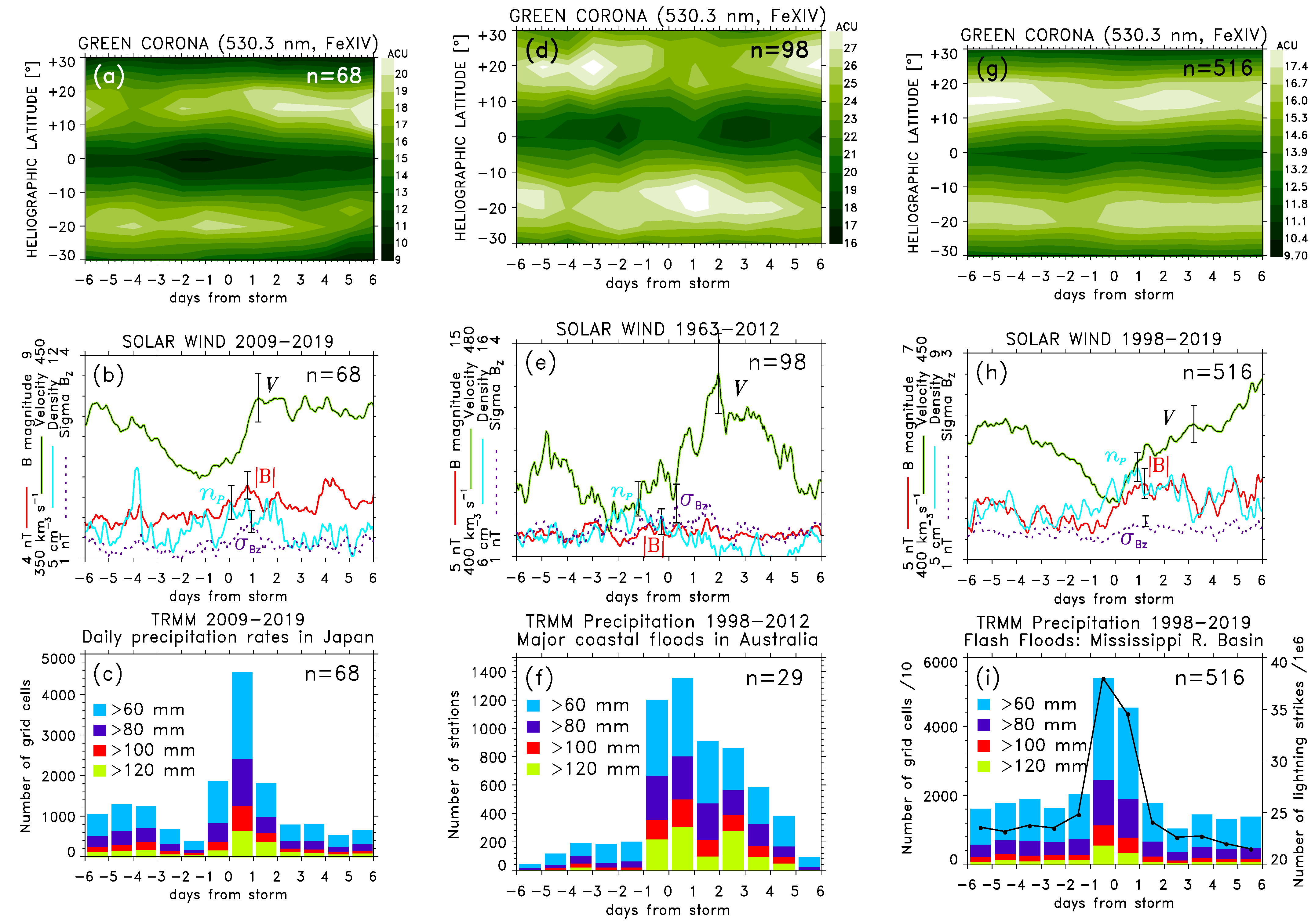
3. High-Rate Precipitation Events in Japan and Solar wind High-Speed Streams

The main causes of heavy precipitation in Japan other than typhoons are intensifications of extratropical cyclones, particularly during the winter season in the form of snow or rain, and activations of a stationary front during the rainy (“tsuyu”) season from early June to mid-July. The explosive development of extratropical cyclones tends to follow arrivals of solar wind HSSs from coronal holes [23]. For example, from December 2017 to January 2018, hourly solar wind data in Figure 1 show several HSS/CIRs (marked with red asterisks) that were followed by explosive development of extratropical cyclones over the North Pacific. One interplanetary coronal mass ejection (ICME) is marked with an orange triangle.
A tracking algorithm on the surface low pressure field from the JRA-55 meteorological re-analysis data [40] was applied and tracks of explosive extratropical cyclones in the North Pacific were obtained [24]. Those considered in Figure 1 reached minimum central pressure < 990 mb and maximum normalized deepening rate NDRr > 0.5. The value of NDRr = 1 represents the relative central pressure change of 24 mb in 24 h at a latitude of 60° (Lim and Simmonds [41]; their Equation (2)), adopted by Prikryl et al. [24]. The open circles shown in Figure 1 are scaled by the maximum normalized deepening rate NDRr of extratropical cyclones over the North Pacific. Most of these explosive developments followed arrivals of major HSS/CIRs and those that affected Japan resulted in precipitation. Maximum TRMM daily rates and the number of TRMM grid cells with daily precipitation rates exceeding 50 mm over Japan are shown at the top. Global satellite images of clouds at 3-hourly intervals are provided by the International Satellite Cloud Climatology Project Global ISCCP B1 Browse System (GIBBS) [42] (https://www.ncdc.noaa.gov/gibbs/html/HIM-8/IR/2017-12-15-00, accessed on 9 September 2021). Himawari-8 infrared images and TRMM precipitation maps can be viewed in Videos S1 and S2 in Supplementary Materials.
An extreme explosive cyclone that reached a minimum central pressure of ~944 mb caused a major snowstorm that affected northern Japan starting December 24. Another major snowstorm that affected Japan also coincided with the arrival of HSS/CIR on 8 January 2018. Precipitation rates also peaked on January 1 and 14 following HSS/CIRs, but they were moderate or low because the extratropical cyclones intensified just east of Japan. The head of the explosive cyclone on January 1 marginally affected precipitation over Hokkaido. Explosive cyclones on 17–18 December developed over the Pacific further north and east of Japan. There are other examples of snowstorms in Japan that can be linked to arrivals of HSS/CIRs, such as a severe snowstorm caused by an explosive cyclone in Hokkaido [43] that coincided with the arrival of a major HSS/CIR on 1 March 2013 (Figure S1 in Supplementary Materials).
Heavy rainfall events during the rainy season in Japan have become more frequent, which has been attributed to climate change. An unprecedented disastrous event occurred in early July 2018 [5,44,45,46]. Although the heavy rainfall occurred over an extensive area of Japan from 28 June to 8 July, with typhoon Prapiroon passing over the western Japan and Japan Sea on 2–4 July, the precipitation maximized during 5–8 July, causing the most damage in the western part of Japan. After the typhoon had passed, a stationary front formed over Japan and its activation resulted in the heaviest rainfall. Figure 2 shows solar wind plasma variables, the maximum daily precipitation (red crosses), the number of TRMM grid cells over Japan with daily precipitation rates exceeding given thresholds (histograms) and Kp-index of geomagnetic activity. The heaviest rainfall (largest number of grids with high precipitation rates) closely followed arrival of a major HSS/CIR, although the maximum daily rate due to Prapiroon passing was observed on July 3. A similar extreme event occurred again in western Japan in early July 2020 [47,48,49]. The highest precipitation rates that were recorded from 3 July to 6 July (e.g., 367 mm in Minamata on 4 July) coincided with the arrival of a major HSS/CIR on July 4. The most recent heavy rainfall events in 2021 (http://floodlist.com/, accessed on 9 September 2021), one in Shizuoka prefecture in 1–3 July, which caused a deadly landslide in Atami, and another in Kagoshima prefecture (e.g., 418 mm in Satsuma) on July 10 also closely followed arrivals of HSS/CIRs on 30 June and 10 July, respectively (https://www.swpc.noaa.gov/products/real-time-solar-wind, accessed on 9 September 2021).
Of course, this is not to suggest that all heavy rainfall events start with arrivals of HSS/CIRs, because there are many known meteorological factors that lead to heavy rainfall. Even the heavy rainfall events that we discussed above may have had already started earlier when all ingredients for heavy precipitation were present, and forecasts and warnings had indeed already been issued. For example, in the early July 2018 case discussed above, the presence of the stationary “Baiu” front and typhoon Prapiroon passing primed the atmospheric conditions, and heavy rainfall occurred prior to 5–6 July [46], but was significantly enhanced following the arrival of the HSS/CIR. It is the tendency of such events to occur following HSS/CIRs that we discuss in this paper. Furthermore, the physical mechanism that is proposed in Section 6 is not limited to HSS/CIRs.
In this section we focused on Japan, but because the subsequent analysis also includes high-rate precipitation events over continental Australia and United States, which have characteristics that may differ from those in Japan, further discussion is provided with Figures S2 and S3, and Videos S3–S7 in Supplementary Materials. While it is known that precipitation is highly variable across the globe and caused by various phenomena, as already discussed in this section, we focus on mid latitudes dominated by extratropical cyclones and convective storms.

4. Superposed Epoch Analysis Keyed to Heavy Rainfall Events Causing Floods or Flash Floods

Pursuing the approach taken in previous studies mentioned in the Introduction, we use the SPE analysis method to show a tendency of heavy rainfall occurrence to follow arrivals of solar wind disturbances, mainly HSS/CIRs but with possible contribution of ICMEs and their upstream sheaths [50,51] enhancing their geo-effectiveness [52].
Focusing on Slovakia, Prikryl et al. [26] showed that events of heavy rainfall causing floods or flash floods tend to follow arrivals of HSS/CIRs. Here we focus on events in Japan, south-eastern coast of Australia and the Mississippi River Basin (MRB) in the United States. Heavy rainfall events in Japan that are listed in the JMA summaries (2009–2019) of severe weather events are supplemented with flash floods in Japan from the FloodList archive (2013–2019). Heavy rainfall events caused by typhoons are excluded, because they result from typhoon landfalls, which are determined by tracks of typhoons that are shaped by atmospheric circulation. The actual intensification of typhoons typically occurs over warm ocean waters, although rapid intensification has been linked to HSS/CIRs [25]. The results of the SPE analysis of time series of the green corona intensity and solar wind variables keyed to start dates of heavy rainfall events in Japan are shown in Figure 3a and Figure 3b, respectively. Figure 3c shows the cumulative number of TRMM grid cells for each epoch day with above-threshold daily precipitation rates over Japan.
Figure 3d,e show the results of the SPE analysis keyed to start days of major coastal floods in south-eastern Australia for the period of 1963–2012 (Callaghan and Power [53]; their Table 1). For the period of 1998–2012 that is covered by the TRMM dataset, Figure 3f shows, for each epoch day, the cumulative number of grid cells with above-threshold daily precipitation rates over the geographic area of the coastal region studied by Callaghan and Power [53] (their Figure 1), including a swath of coastal ocean.
As will be shown in Section 5, if the SPE analysis is keyed to HSS/CIR arrivals, smoothed mean variations of solar wind parameters with sharp peaks at the key time in solar wind density, np, magnetic field magnitude, B, and standard deviation of the magnetic field north–south component, σBz, followed by high mean solar wind velocity, V, are obtained, e.g., (Prikryl et al. [26]; their Figure 5).
However, if the key days are defined by start dates of storms mostly distributed around, or following HSS/CIRs, with some of the storms possibly occurring even several days before or after HSS/CIRs, the SPE analysis will still obtain similar patterns, i.e., peaks in np, B, and σBz around the key day followed by an increase in V of smaller amplitude. This is the case for the SPE analysis results shown in Figure 3b,e. In both cases the SPE analysis results show the mean V rising from a minimum before the key day followed by a maximum after the key day, with peaks in np, B, and σBz around the key day. This is the result of superposition of HSS/CIRs most of which were near, or preceded the key events, i.e., not necessarily coinciding with the key events. Similarly, the SPE analysis of the green corona intensity (Figure 3a,d) shows depletions of the mean intensity at low heliographic latitudes, which is the result of superposition of misaligned coronal holes. These results indicate a tendency of heavy rain and major floods to follow arrivals of HSS/CIRs from coronal holes. If the key days were randomly distributed relative to HSS/CIRs the mean variations would be expected to have random phases or be completely smoothed out (flat) for large number of events, n. Neither is the case, and the similar above-described patterns are consistently obtained.
This is further demonstrated for flash floods in the United States (Figure 3g–i). From the NOAA/NWS storm database records of flash flood reports, we build time series of the daily sum of flash flood events for each MRB state (MN, WI, IA, IL, MO, KY, TN, MS, and LA) and use it to define “flash flood outbreak” dates to be used as key days for the SPE analysis of solar wind parameters. A threshold cutoff daily sum of at least five reports is used to define the start and end days of a “flash flood outbreak” period, with a daily sum peak of at least 10 events and the rest of the days within the period also remaining above the threshold cutoff. The start days of the “flash flood outbreak” periods for all MRB states combined are used in the SPE analysis of the green corona intensity and solar wind parameters shown in Figure 3g,h, respectively. For each epoch day, Figure 3i shows the cumulative number of grid cells with above-threshold TRMM daily precipitation rates over the MRB region, defined as a rectangle delimited by latitudes and longitudes containing all MRB states. In addition, using the SWDI data for the continental United States, the cumulative number of lightning strikes over the MRB region is shown. The SPE analysis results (Figure 3g,f) are similar to those for the cases of Japan and Australia, indicating a tendency of the flash floods to follow arrivals of HSS/CIRs that was already discussed in Section 3.
In Section 5, we provide more direct statistical evidence of high-rate precipitation increase following HSS/CIRs by inverting the SPE analysis approach by choosing HSS/CIR arrivals as key times, instead of the storm start dates. The times of CIRs are defined by fast/slow stream interfaces observed upstream from Earth as described in Section 2.

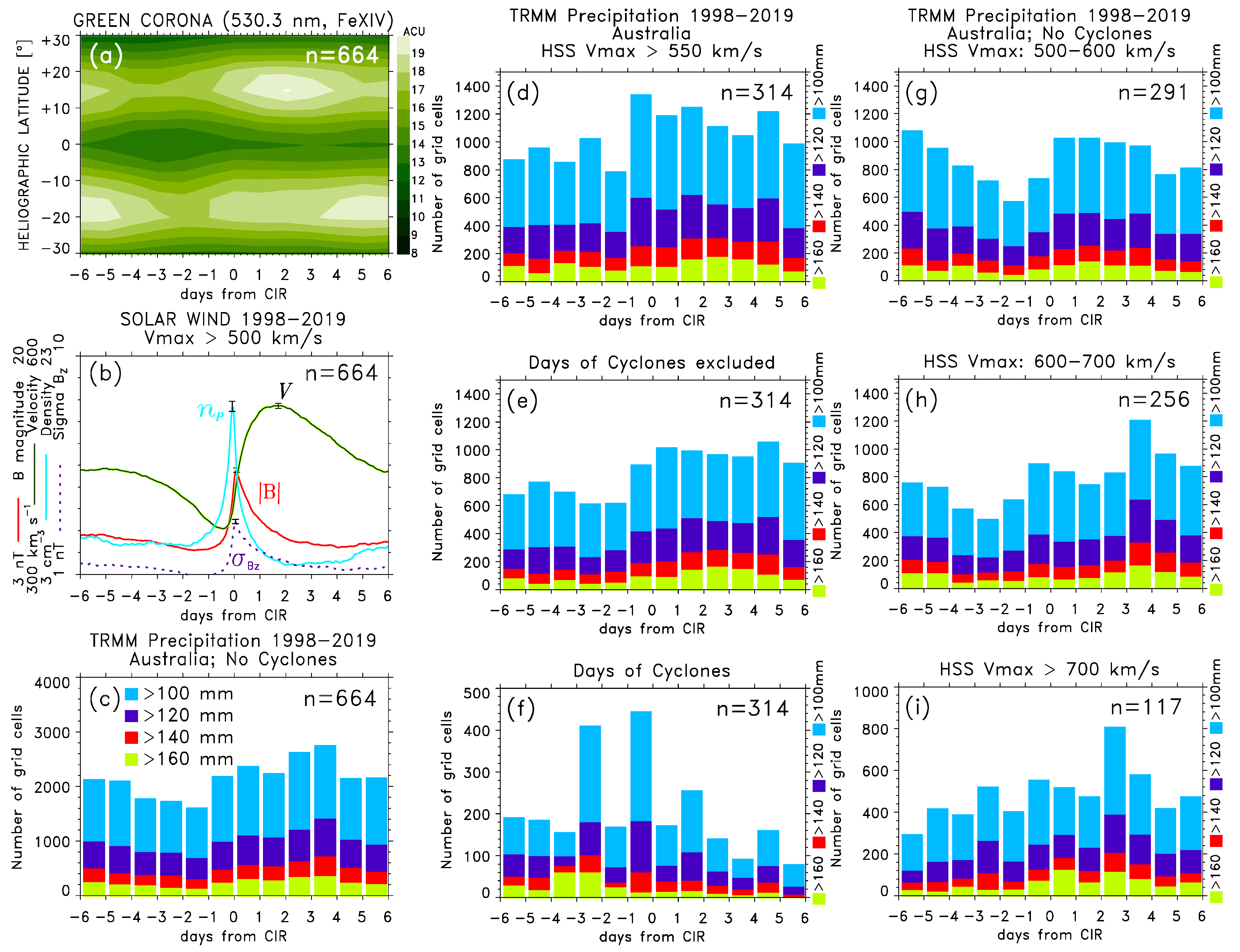
5. Modulation of High-Rate Precipitation Occurrence by High-Speed Streams

5.1. SPE Analysis Keyed to Arrivals of Major HSS/CIRs

To examine the statistical occurrence of high-rate precipitation in Japan relative to arrivals of HSS/CIRs, the SPE analysis is keyed to arrival times of major HSS/CIRs. The TRMM dataset of gridded daily precipitation rates over Japan, focusing on high daily precipitation rates exceeding four thresholds of 100, 120, 140, and 160 mm, is used. For major HSSs in the period of 1998–2019 reaching a maximum solar wind velocity Vmax > 700 km/s, Figure 4a,b shows the SPE analysis results for the green corona intensity and solar wind parameters, respectively. As expected, the superposition of HSS/CIRs relative to the well-defined interface between the fast and slow solar wind results in sharp peaks in the mean np, B, and σBz close to the key time, while the mean solar wind velocity V is rising from a minimum before to a maximum after the key time (Figure 4b), with the mean coronal hole preceding it by about 4 days.
Of main interest in this analysis are total cumulative numbers of grid cells where daily precipitation rates exceeded given thresholds, summed up for each epoch day relative to the key time. They show a large increase at epoch day 0, with the arrival of these very fast HSS/CIRs (Figure 4c). Precipitation during days when typhoons approached or impacted Japan obtained from the best-track database of West Pacific typhoons are excluded, because tropical cyclones evolve (intensify or weaken) over the ocean, and landfall events themselves, though causing heavy rainfall over land, are generally unrelated to HSS/CIR. Very similar results are obtained using the rain-gauge based APHRODITE dataset (1998–2015) [54] over Japan (Figure S4 in Supplementary Materials).
Figure 4d–f shows the SPE analysis results (omitting plots of the mean green corona intensity and solar wind parameters) for Vmax > 650 km/s, which almost doubles the number of key times, n. There are three main reasons why it is important to vary n and group the analysis by Vmax. First, larger n should yield higher statistical significance for the SPE results. Second, faster HSSs usually result in stronger MIA coupling, although other solar wind parameters, in particular IMF Bz, are often more important. Third, it allows consistency of the SPE results for different grouping or subperiods to be checked. The cumulative numbers of TRMM grid cells with high precipitation rates relative to arrival of HSS/CIRs are shown for all days including typhoon days (Figure 4d), for days with typhoons excluded (Figure 4e), and for typhoon days only (Figure 4f). With or without typhoon days (Figure 4d,e), the histogram peak on days adjacent to the key time (day −1 or 0), i.e., on either side of the HSS/CIR interface. With typhoon days removed, the peak shifts to day 0. It should be noted that key times are based on the hourly solar wind dataset, while daily precipitation rates are used from the TRMM dataset in this analysis, i.e., the daily TRMM rates are matched with hourly solar wind parameters at 0 UT. Figure 4g–i shows the SPE analyses for three intervals of Vmax, with typhoons excluded in all three cases. While there are high precipitation rates during the descending phase of HSSs that precede the arrivals of the key HSS/CIRs, particularly for the lower-velocity HSSs (Figure 4g), they decrease to a minimum at epoch days ≤ −1, which is then followed by an increase to the next maximum. For progressively faster/stronger HSS/CIRs, the occurrence of high precipitation rates peaks on days adjacent to the key time (Figure 4h,i).
In Figure 5, which is structured similarly to Figure 4, the statistical relationship between solar wind HSS/CIRs and TRMM precipitation rates over the continental Australia is examined. For HSSs with maximum solar wind velocity Vmax > 500 km/s (Figure 5c), the SPE analysis shows an increase in the occurrence of high-rate precipitation from the minimum before, to a maximum after, the arrival of HSS/CIRs with days of tropical cyclone impacts excluded from cumulative counts. In the middle column (Vmax > 550 km/s), this is shown for the case with tropical cyclone days included (Figure 5d) and excluded (Figure 5e), while the cumulative counts are limited to days of tropical cyclones in Figure 5f. Further grouping of the SPE analysis by Vmax (Figure 5g–i), with tropical cyclone days excluded, confirms a general increase in high precipitation occurrence following arrivals of HSS/CIRs.
The larger geographical area of the continental U.S. should provide even more statistically significant results (Figure 6), because of larger number of TRMM grid cells, larger geographical area targeted by potential solar wind MIA coupling process (see, Section 6), and a greater variety of climates and weather patterns. For HSSs with maximum solar wind velocity Vmax > 600 km/s (Figure 6b), the SPE analysis result shows the high-precipitation occurrence reaching a broad maximum during the declining phase of the preceding HSSs, dropping to a minimum on day 0, and then rising to a maximum 2 days later following arrivals of major HSS/CIRs. This pattern is correlated with the mean solar wind velocity with a lag of about 1 day. The case of Vmax > 400 km/s, which more than doubles the number of key times n as well as the cumulative numbers of days with above-threshold precipitation rates, gives similar results with hurricane days included (Figure 6d), or excluded (Figure 6e), i.e., a correlation between the mean V and the high-rate precipitation occurrence lagged by about 1 day. Further grouping of the SPE analysis by Vmax (Figure 6g–i), with hurricane days excluded, reproduces a general pattern of an increase in high-rate precipitation occurrence from a minimum to maximum following arrivals of HSS/CIRs, although the minima are shifted to day 0, or by about 1–2 days when compared with the results in Figure 4 and Figure 5.
As already discussed in Section 3, heavy precipitation in Japan closely follows intensifications of extratropical cyclones or activations of stationary fronts over Japan. In Australia, east coast lows and frontal systems of extratropical cyclone intensifying south-west of Australia are closely followed by heavy precipitation. In comparison, in the continental U.S. (Figure S2 in Supplementary Materials), heavy rainfall on the west coast is mainly caused by extratropical cyclones that form and intensify over Pacific before they impact the west coast. Intensifications of Colorado lows and nor’easters may also take a couple of days before they produce the heaviest precipitation in the east and north-east. This can explain the delayed response of heavy precipitation following the HSS/CIRs arrivals.
The results for the TRMM high-rate precipitation occurrence are further supported using the SWDI/NLDN data for the continental United States. Though not the focus of this analysis the cumulative numbers of lightning strikes over the CONUS region show patterns that are similar to those for high-rate precipitation, because heavy rainfall is sometimes accompanied with lightning activity (thunderstorms).
The conclusion is that, statistically, there is a tendency for the occurrence of high precipitation rates to increase following the arrivals of HSS/CIRs, which is consistent with the results discussed in Section 3 and Section 4.

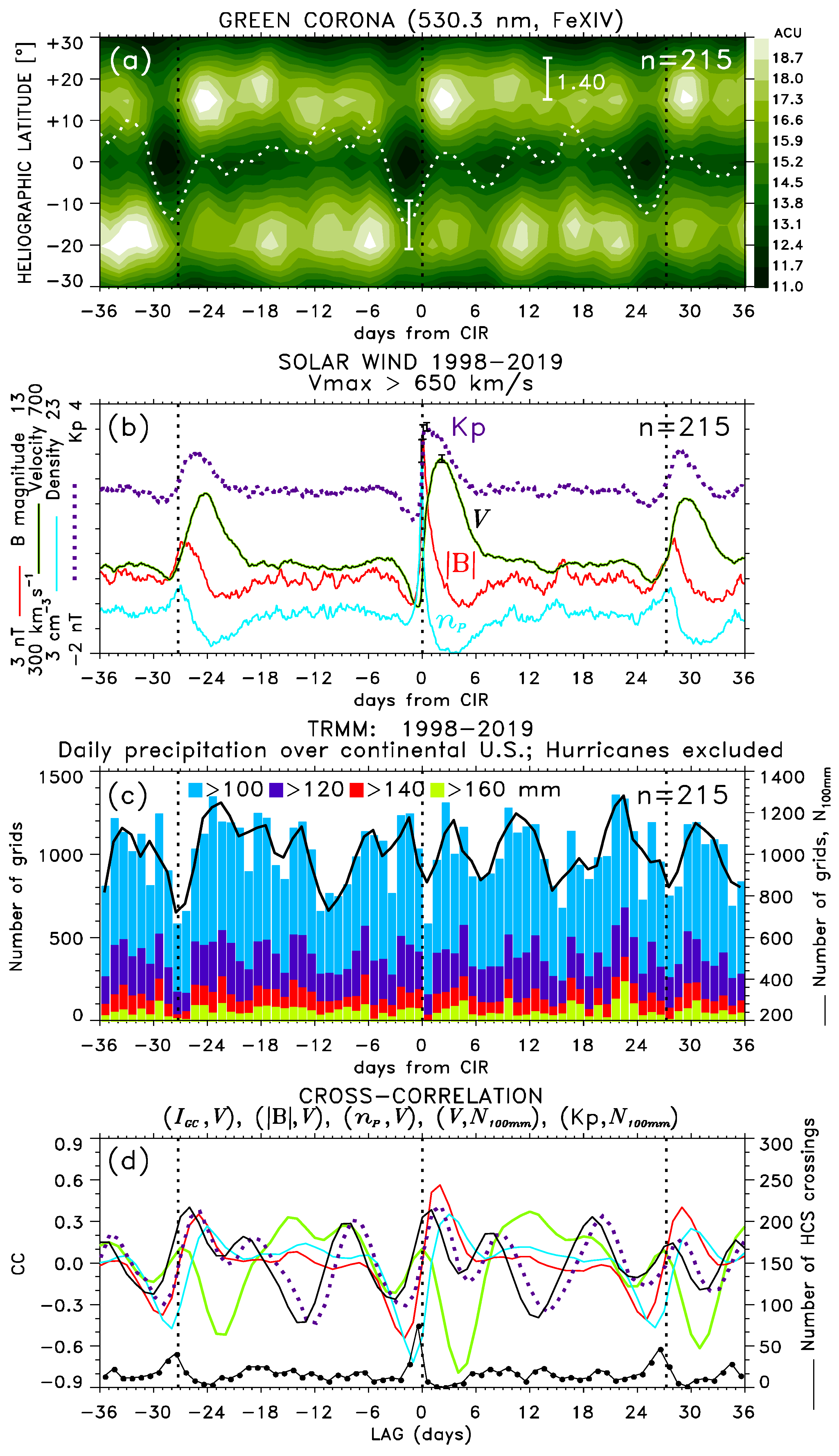
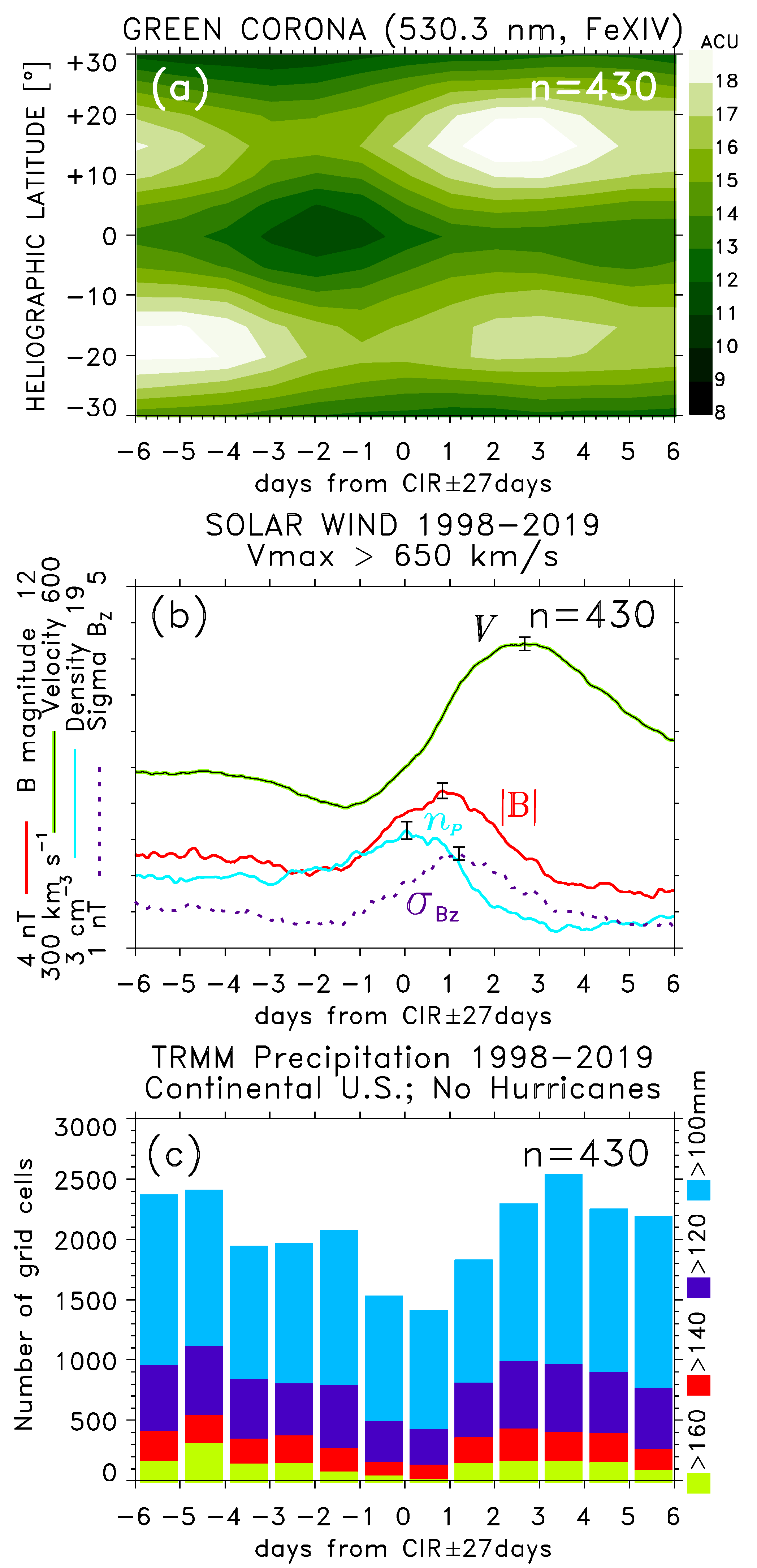
5.2. The SPE Analysis Extended to ±36 Days from Arrivals of Major HSS/CIRs

HSSs emanating from polar coronal holes persist for years [31,55] and cause recurrent geomagnetic activity [52,56] and magnetic storms [57]. Coronal holes that extend to low latitudes because of the warped heliospheric current sheet (HCS) [29,30], and self-contained circular coronal holes that sometimes form at low latitudes, can persist for many solar rotations resulting in recurrent HSSs.
To examine the influence of recurrent HSS/CIRs, the SPE analysis is extended to a time interval of ±36 days from the arrival time of major HSSs/CIRs (Figure 7). Instead of σBz, which always results in a pattern that is very similar to B, we now include the Kp-index of geomagnetic activity. The vertical dotted lines are shown for the key time and the key time ±27.28 days (the synodic or Carrington rotation). The superposition of recurrent coronal holes, which include north and south coronal holes, results in depressions of the mean green corona intensity IGC (Figure 7a) that are, in this case, centered at about zero heliographic latitude and, on average, 2–3 epoch days before arrival times of recurrent HSSs. The mean IGC averaged over heliographic latitudes between −30° and +30°, with the mean value over the period of 72 days subtracted, is shown by a white dotted line. The standard error bar for one of the IGC minima, and the ordinate scale bar corresponding to the color scale on the right, are also shown. Figure 7b shows the superposition average of Kp-index and solar wind plasma variables, all showing the principal maxima following the key time and secondary maxima due to recurrent HSS/CIRs at ±27 epoch days. As expected, the mean Kp-index is well correlated with the mean solar wind velocity V, but steeply increases from a minimum before, to a maximum just after the key time, which is similar to the mean np, B, and σBz.
As in Figure 6i, but now for ±36 days from the key time, Figure 7c shows the cumulative number of TRMM grid cells over the continental U.S. with above-threshold daily precipitation rates, N100mm, N120mm, N140mm, and N160mm. The bold black line shows N100mm smoothed by a three-point running window. The histograms show not only the increase in precipitation from a minimum at day 0 to a maximum at day +2 (already shown in Figure 6i), but also similar patterns one solar rotation before and after the key time, i.e., increases in precipitation from minima around the mean arrival time of recurrent streams to maxima 2–3 days later. We now compare variations among six variables (V, IGC, np, B, Kp and N100mm). The cross-correlation functions (CCFs) that are computed for the mean solar wind velocity V paired with the rest of the variables (Figure 7d) are shown in colors corresponding to those in Figure 7b. The CCF (IGC, V) that is shown in the green line representing IGC has the largest inverse correlation showing the principal minimum at lag +4 days (CC = −0.83). The secondary minima at lags of −22.5 and +31 days, i.e., lags +4.5 and +4 day relative to vertical dotted lines represent recurrent streams. These lags represent mean propagation times of HSSs from coronal holes to the maxima in V observed upstream from the Earth. On the other hand, CCF (B, V) and (np, V) show principal and secondary maxima at lags relative to vertical dotted lines of ~2 and 3 days, respectively, which relate to arrivals of CIRs, i.e., the interfaces between the fast and slow solar wind.
Of main interest in this paper are the correlations with high-rate precipitation. The principal peak and one secondary peak of the CCF (V, N100mm) are at lags of +1 and −26 day (CC = 0.40). The CCF (Kp, N100mm) has a similar shape, but is shifted by 1 day, showing slightly higher maximum correlation coefficient (CC = 0.43 at lag +2). However, the main observation here is that there are minima in N100mm at −27, 0, and +27 epoch days followed by maxima in high precipitation occurrence a couple of days later. This is the main reason for the correlations of V and Kp with N100mm. Although there are other pronounced N100mm minima near −12 and +15 epoch days followed by maxima that are 27 days apart, in these cases the mean V goes through a very shallow insignificant minima accentuated by small peaks in np and B, and a very small increase in Kp. However, the averaged corona intensity IGC shows small intensity depletions between the main minima (Figure 7a). We will return to this point at the end of this section and in Section 6.
These quantitative results further support the observations discussed with Figure 1, Figure 2, Figure 3, Figure 4, Figure 5 and Figure 6 and confirm the tendency of an increase in precipitation rates following the arrivals of HSS/CIRs, including the recurrence with periodicity of 27 days. The latter is further demonstrated in Figure 8 that shows the SPE analysis (limited to ±6 days relative to newly defined key time) of the green corona intensity, solar wind variables, and cumulative number of grids with above-threshold daily precipitation rates. The time series are now keyed to times that are shifted by ±27 days relative to the actual arrival times of HSS/CIRs, which are used as key times in Figure 6i and Figure 7, thus doubling the number n of superposed epochs. Expectedly, Figure 8a,b shows smaller amplitudes and broader peaks, because of averaging “imperfectly” recurrent streams (coronal holes and streams evolve over one solar rotation, shifting in longitude and arrival times, respectively). However, the amplitude of the increase in N100mm almost doubles (factor 1.7) compared to Figure 6i, since the total cumulative sum of high-precipitation grids is now for two returns of the recurrent streams separated approximately by 54 days. If the SPE analysis is repeated with key times lagged by ±54 days from the actual HSS/CIRs arrivals, the results are very similar, but the amplitude is increased by a factor 1.4 (not shown) comparing to Figure 6i, even though the superposed recurrent streams are separated by approximately 108 days.
Of course, HSS/CIRs and their sources, coronal holes, are more often spaced by less than 27 days, typically by 9 or 13.5 days, depending on how many coronal holes cross the solar meridian in one solar rotation. Because the spacing varies over a period of many years (Figure 7), the SPE analysis averaging smears these intermediate variations due to shifts in the position of coronal holes and times of corresponding HSS/CIRs. However, N100mm, N120mm, N140mm, and N160mm, which are not averages, show intermediate variations, and secondary CCFs peaks at lags between −27 and +27 days. As already discussed above, some of these variations can be associated with small variations in the averaged variables (Figure 7a,b), particularly the corona intensity that shows traces of averaged intermediate coronal holes. However, their amplitudes are enhanced if the SPE analysis is limited to years that were dominated by several recurrent coronal holes and corresponding solar wind streams.
Recurrent coronal holes, which are quite regularly spaced in heliographic longitude, are often present during the descending phase of the solar cycle and around solar minima. de Toma [58] analyzed coronal holes during the extended minimum between Cycles 23 and 24 and examined the consequences for the solar wind speed near the Earth. Two or three low-latitude coronal holes per solar rotation were observed by SOHO/EIT in 2008 separated by about 110° to 120° in longitude [58] (their Figures 5 and 6; CHs located at longitudes ~140° and 260° in March–April 2008, ~200° and 310° in September–October 2008, ~120°, 230°, and 330° in December 2008 to January 2009, and 60° and 180° in June–July 2009). During the anomalous, prolonged solar minimum at the end of Cycle 23, these low-latitude coronal holes remained a significant source of solar wind, particularly in 2008, producing fast recurrent solar wind streams [59,60]. Spectral analysis of solar wind data and geomagnetic activity Kp index in 2008 showed strong peaks at 9 and 13.5 days [61].
Keyed to major HSS/CIRs with Vmax > 500 km/s, the SPE analysis of the green corona intensity averaged over the period 2008-2009 shows a series of predominantly southern coronal holes (Figure 9a), with the mean IGC (white dotted line) averaged over heliographic latitudes between −30° and +10° shown. The corresponding mean solar variables (Figure 9b) show recurrent HSS/CIRs spaced by ~9 days, on average. High-rate precipitation numbers N100mm, N120mm, N140mm, and N160mm, as well as the three-point running average of N100mm (Figure 9c) show variations that are very similar to those of mean solar corona intensity, solar wind variables and Kp index (Figure 9b). The CCFs computed for V paired with IGC, np, B, and the smoothed N100mm, as well as CCF (Kp, N100mm), all display principal and several secondary peaks spaced by 9 days (Figure 9d). In particular, the CCFs (B, V), which is almost identical with CCF (σBz, V) (not shown), is similar to CCF (V, N100mm) and CCF (Kp, N100mm), apart from the shift, with the maxima in correlation coefficients of 0.72, 0.47, and 0.45 at lags +1, +2, and +3 days, respectively. The CCF (np, V) also show moderate correlation peaks at lags that are similar to those of CCF (Kp, N100mm). The CCF (IGC, V) shows much more pronounced positive correlation peaks than those shown in Figure 7d, although again the highest inverse (negative) correlations are physically meaningful, with the lags determined by the mean propagation time of HSSs from coronal holes.
The HSSs from coronal holes are anchored in the large-scale solar magnetic field structure that is extended into the interplanetary space by solar wind [62]. The magnetic sector boundaries that have been identified as heliospheric current sheet (HCS) often precede the high-speed stream interfaces (HSS/CIRs) by about 1 day, unless the two coincide. At the bottom of Figure 7d and Figure 9d, cumulative numbers of HCS crossings for each epoch day show peaks preceding the key time (CIRs) by 1 day or less, and similar peaks for the recurrent HSS/CIRs at ±27 epoch days, as well as the intermediate HSS/CIRs in Figure 9b. If the key times in the SPE analysis are defined by the HCS crossings instead of CIRs, the results are similar to those in Figure 9, although the correlation coefficients at the principal and secondary lags of CCFs (V, N100mm) and (Kp, N100mm) are lower (Figure 10). Nevertheless, N100mm shows a minimum at about the epoch day +1, as well as minima near epoch days ±27, that are followed by maxima a few days later. Remarkably, the variations of the mean green corona intensity, solar wind variables, as well as high-rate precipitation occurrence all display a clear periodicity of about 9 days, as confirmed by CCFs. These results are similar to the Wilcox effect [21], which is further discussed in Section 6.

6. Discussion

We have examined high-rate precipitation leading to floods and flash floods in Japan, Australia, and the continental U.S. in the context of solar wind, linking the occurrence of such weather events to arrivals of solar wind HSS/CIRs. The geo-effectiveness of HSSs/CIRs is well known [56,57] and associated with high-intensity, long-duration continuous auroral electrojet activity (HILDCAA) depositing substantial energy to the auroral zone [63]. HILDCAAs are caused by trains of solar wind Alfvén waves [64] that couple to the magnetosphere–ionosphere system [65,66]. Solar wind MIA coupling generates medium- to large-scale AGWs globally propagating from sources in the lower thermosphere at high latitudes both upward and downward [67,68,69,70,71]. The coupling is most intense when the HSS/CIRs and/or interplanetary shocks at the leading edges of ICMEs arrive and generate large-amplitude AGWs originating in the lower thermosphere at high latitudes. Solar wind magneto-hydrodynamic waves, including Alfvén waves, modulate the high-latitude ionospheric currents that generate globally propagating AGWs, which can reach the troposphere with significantly attenuated amplitudes [72]. However, conditional moist instabilities, particularly moist symmetric instability (MSI) [9] only require very small displacements of moist air to initiate slantwise convection. Prikryl et al. [22] suggested that in the extratropical cyclone warm frontal zone, with warm air advection over the cool air mass ahead, the over-reflecting gravity-wave-induced vertical lift may trigger/release MSI at near-threshold conditions leading to precipitation bands. Prikryl et al. [22,24,26] presented several cases of series of rainbands or convective cells suggesting that they were triggered by incoming aurorally generated AGWs.
Theoretical analysis of AGW propagation in the lower atmosphere using an expansion in three-dimensional normal mode functions was performed by Hagiwara and Tanaka [73]. These authors showed that the waves can propagate downward to the troposphere as attenuating gravity waves and “the wave propagations and reflections at the surface create an anti-node of geopotential at the bottom of the atmosphere corresponding to the vertical width of the initial state of the impact.” On the other hand, “standing waves in temperature create a node at the ground surface.” They suggested that standing waves generated in the lower troposphere could affect atmospheric stability through the passage of gravity waves, in turn affecting the development of cyclones.
The SPE analysis of green corona intensity and solar wind parameters is performed using a twofold approach. In Section 4, the SPE analysis keyed to significant rainfall/flood events indicated a tendency of these flood events to follow arrivals of solar wind HSS/CIRs. In Section 5, the key times are defined by the solar wind events, which are either arrival times of major HSS/CIRs, or HCS crossings. The SPE analysis results show an increase in the occurrence of high-rate precipitation rates following the key time. In the case of the continental U.S., the SPE analysis extended to ±36 days about the key times reveals a similar response at epoch days ±27 due to recurrent streams.
The cross-correlation analysis of the superposed-epoch averages of the green (Fe XIV, 530.3 nm) corona intensity, solar wind variables, as well as Kp-index of geomagnetic activity with high-rate precipitation occurrence show the principal and two secondary correlation peaks at lags ±27 days relative to the principal peak that are attributed to recurrent high-speed streams. When the analysis is limited to the years 2008–2009 around the solar minimum, correlation peaks spaced by about 9 days are found, which is a result of the high-speed streams emanating from recurrent coronal holes spaced by ~120° in heliographic longitude.
As pointed out in Section 5, these results are comparable with the Wilcox effect obtained by superposed epoch analysis of vorticity area index (VAI), a measure of storminess, keyed to heliospheric current sheet (magnetic sector boundary) crossings, which usually closely precede or coincide with stream interfaces, thus supporting the conclusion that high-speed streams modulate the occurrence of high-rate precipitation at mid-latitudes. The SPE analysis results in Figure 10, i.e., that the minima in the occurrence of high-rate precipitation, N100mm, near +1 and ±27 epoch days, which are followed by maxima a few days later, are similar to the Wilcox effect [15,16,21,74] that showed the VAI minimum about one day after the HCS crossings, although no reference to the maxima in the VAI that followed a few days later was made. Additionally, the SPE analysis of VAI, extended to ±30 days by Prikryl et al. [21] (their Figures 2 and 3), showed VAI minima following the recurrent streams, as well as intermediate minima coinciding with intermediate coronal holes, confirming the results by Wilcox et al. [74] (their Figure 4). The main VAI minimum was linked to a calm solar wind period characterized by a weak magnetic field and absence of Alfvén waves [21] referred to as the “calm before the storm” in CIR/magnetosphere interactions [75]. The minimum in the occurrence of high-rate precipitation appears to correspond to the minimum in “storminess” characterized by the VAI, while the maximum in VAI represents a maximum in storminess. However, observations of the Wilcox effect were limited to winter months; therefore, the similarity with the present results ends there.

7. Conclusions

Consistently with previously published results, it is shown that heavy rainfall events leading to floods and flash floods in Japan, Australia, and the continental U.S. tend to follow arrivals of high-speed solar wind streams. The superposed epoch analyses keyed to major high-speed streams show increases in high-rate precipitation, based on rain-gauge- and satellite-based gridded precipitation data, following arrivals of high-speed streams, including recurrence with periodicity of 27 days. When the analysis is limited to years around the solar minimum (2008–2009), which was dominated by recurrent coronal holes separated by ~120° in heliographic longitude, the results for both the solar wind and high-rate precipitation reveal periodicity of 9 days. These results are similar to the Wilcox effect for vorticity area index. Further theoretical and computational studies of possible physical mechanisms to explain these observations, including the influence of aurorally generated gravity waves on tropospheric weather, are needed to complement the data-driven analysis of this phenomenon.

Supplementary Materials

The following are available online at https://www.mdpi.com/article/10.3390/atmos12091186/s1, Figure S1: Snowstorms in Japan in March 2013, Figure S2: Solar wind and high-rate precipitation over continental Australia and United States, Figure S3: A major coastal flood in Australia and a flash flood in the Mississippi River Basin, Figure S4: The SPE analysis of high-rate precipitation from the APHRODITE dataset, Video S1: GIBBS Himawari-8 images for Figure 1, Video S2: TRMM maps for Figure 1 (Japan), Video S3: GIBBS Himawari-8 images for August 2015, Video S4: TRMM maps for the Australian sector, Video S5: GIBBS GOES-8 images for January 1999, Video S6: GIBBS GOES-10 images for January 1999, Video S7: TRMM maps for North America.

Author Contributions

Conceptualization, P.P., V.R. and E.A.P.; methodology, P.P. and V.R.; software, P.P.; validation, P.P. and V.R.; formal analysis, P.P.; investigation, P.P., V.R. and E.A.P.; resources, P.P., V.R. and E.A.P.; data curation, P.P. and V.R; writing—original draft preparation, P.P.; writing—review and editing, P.P., V.R. and E.A.P.; visualization, P.P.; supervision, P.P. All authors have read and agreed to the published version of the manuscript.

Funding

This research has been supported by the Slovak Academy of Sciences, under VEGA project No. 2/0048/20.

Institutional Review Board Statement

Not applicable.

Informed Consent Statement

Not applicable.

Data Availability Statement

All sources of data are described and referenced by URLs in Section 2.

Acknowledgments

This research was supported by the University of New Brunswick and by the VEGA project 2/0048/20 (Slovak Academy of Sciences). Contributions by the ACE, Geotail, IMP-8, SoHO and Wind spacecraft teams, the NSSDC OMNIWeb projects are acknowledged. Meteorological data were accessed online at web pages provided by various institutions including Japan Meteorological Agency (JMA), Australian Government Bureau of Meteorology, the University of Wisconsin-Madison Space Science and Engineering Center and the University of Washington, Department of Atmospheric Sciences. Copernicus, previously known as GMES (Global Monitoring for Environment and Security), is the European Programme for the establishment of a European capacity for Earth Observation. It funds the project FloodList, the European system for Earth monitoring and reporting floods and flooding news since 2008. The Tropical Rainfall Measuring Mission (TRMM) Multi-Satellite Precipitation Analysis TMPA (3B42) Precipitation (version 7) was produced at Goddard Earth Sciences Data and Information Services Center (GES DISC). APHRODITE project is a collaboration with the Research Institute for Humanity and Nature and the Meteorological Research Institute of the Japan Meteorological Agency.

Conflicts of Interest

The authors declare no conflict of interest.

Abbreviations

The following abbreviations are used in this manuscript:
MIAMagnetosphere-Ionosphere-Atmosphere
HSSHigh-Speed Stream
AGWAtmospheric Gravity Wave
CIRCo-rotating Interaction Regions
HCSHeliospheric Current Sheet
ICMEInterplanetary Coronal Mass Ejection
ACUAbsolute Coronal Unit
SPE Superposed Epoch
NDRNormalized Deepening Rate
CCFCross-Correlation Function
VAIVorticity Area Index
HILDCAA High-Intensity, Long-Duration Continuous Auroral Electrojet Activity
ULF Ultra-Low Frequency
TFMTransfer Function Model
SOHOSolar and Heliospheric Observatory
JMAJapan Meteorological Agency
AMeDAS Automated Meteorological Data Acquisition System
APHRODITEAsian Precipitation Highly Resolved Observational Data Integration towards Evaluation
TRMM Tropical Rainfall Measuring Mission
MWRA Monthly Weather Review—Australia
MRBMississippi River Basin
NOAANational Oceanic and Atmospheric Administration
NWSNational Weather Service
CONUSContinental U.S.
NCEINational Centers for Environmental Information
SWDI Severe Weather Data Inventory
NLDNNational Lightning Detection Network

References

  1. Gaume, E.; Bain, V.; Bernardara, P.; Newinger, O.; Barbuc, M.; Bateman, A.; Blaškovičová, L.; Bloschl, G.; Borga, M.; Dumitrescu, A.; et al. A compilation of data on European flash floods. J. Hydrol. 2009, 367, 70–78. [Google Scholar] [CrossRef] [Green Version]
  2. Carlton, E.J.; Eisenberg, J.N.S.; Goldstick, J.; Cevallos, W.; Trostle, J.; Levy, K. Heavy rainfall events and diarrhea incidence: The role of social and environmental factors. Am. J. Epidemiol. 2014, 179, 344–352. [Google Scholar] [CrossRef] [PubMed] [Green Version]
  3. Kaiser, M.; Borga, M.; Disse, M. Occurrence and characteristics of flash floods in Bavaria (Germany). In Climate Change Management; Leal Filho, W., Nagy, G., Borga, M., Chávez Muñoz, P., Artur, M., Eds.; Springer: Berlin/Heidelberg, Germany, 2020; pp. 293–310. [Google Scholar]
  4. Du, W.; Fitzgerald, G.J.; Clark, M.; Hou, X.-Y. Health impacts of floods. Prehospital Disaster Med. 2010, 25, 265–272. [Google Scholar] [CrossRef] [PubMed]
  5. Bandaru, S.; Sano, S.; Shimizu, Y.; Seki, Y.; Okano, Y.; Sasaki, T.; Wada, H.; Otsuki, T.; Ito, T. Impact of heavy rains of 2018 in western Japan: Disaster-induced health outcomes among the population of Innoshima Island. Heliyon 2020, 6, e03942. [Google Scholar] [CrossRef] [PubMed]
  6. National Academies of Sciences, Engineering, and Medicine. Framing the Challenge of Urban Flooding in the United States; National Academies Press: Washington, DC, USA, 2019; ISBN 978-0-309-48961-4. [Google Scholar]
  7. Houze, R.A. Mesoscale convective systems. Rev. Geophys. 2004, 42, RG4003. [Google Scholar] [CrossRef] [Green Version]
  8. Doswell, C.A.; Brooks, H.E.; Maddox, R.A. Flash flood forecasting: An ingredients-based methodology. Weather Forecast. 1996, 11, 560–581. [Google Scholar] [CrossRef]
  9. Schultz, D.M.; Schumacher, P.N. The use and misuse of conditional symmetric instability. Mon. Weather Rev. 1999, 127, 2709–2732. [Google Scholar] [CrossRef]
  10. Schumacher, R.S. Heavy rainfall and flash flooding. In Oxford Research Encyclopedia of Natural Hazard Science; Oxford University Press: Oxford, UK, 2017. [Google Scholar]
  11. Doswell, C.A.; Bosart, L.F. Extratropical synoptic-scale processes and severe convection. Meteorol. Monogr. 2001, 50, 27–70. [Google Scholar] [CrossRef]
  12. Villarini, G.; Krajewski, W.F.; Ntelekos, A.A.; Georgakakos, K.P.; Smith, J.A. Towards probabilistic forecasting of flash floods: The combined effects of uncertainty in radar-rainfall and flash flood guidance. J. Hydrol. 2010, 394, 275–284. [Google Scholar] [CrossRef]
  13. Gourley, J.J.; Erlingis, J.M.; Hong, Y.; Wells, E.B. Evaluation of tools used for monitoring and forecasting flash floods in the United States. Weather. Forecast. 2012, 27, 158–173. [Google Scholar] [CrossRef] [Green Version]
  14. Schroeder, A.J.; Gourley, J.J.; Hardy, J.; Henderson, J.J.; Parhi, P.; Rahmani, V.; Reed, K.; Schumacher, R.; Smith, B.; Taraldsen, M.J. The development of a flash flood severity index. J. Hydrol. 2016, 541, 523–532. [Google Scholar] [CrossRef] [Green Version]
  15. Wilcox, J.M.; Scherrer, P.H.; Svalgaard, L.; Roberts, W.O.; Olson, R.H. Solar magnetic sector structure: Relation to circulation of the Earth’s atmosphere. Science 1973, 180, 185–186. [Google Scholar] [CrossRef]
  16. Wilcox, J.M.; Scherrer, P.H.; Svalgaard, L.; Roberts, W.O.; Olson, R.H.; Jenne, R.L. Influence of solar magnetic sector structure on terrestrial atmospheric vorticity. J. Atmos. Sci. 1974, 31, 581–588. [Google Scholar] [CrossRef] [Green Version]
  17. Taylor, H.A. Selective factors in Sun-weather research. Rev. Geophys. 1986, 24, 329–348. [Google Scholar] [CrossRef]
  18. Lam, M.M.; Tinsley, B.A. Solar wind-atmospheric electricity-cloud microphysics connections to weather and climate. J. Atmos. Sol. Terr. Phys. 2016, 149, 277–290. [Google Scholar] [CrossRef] [Green Version]
  19. Tsurutani, B.T.; Hajra, R.; Tanimori, T.; Takada, A.; Remya, B.; Mannucci, A.J.; Lakhina, G.S.; Kozyra, J.U.; Shiokawa, K.; Lee, L.C.; et al. Heliospheric plasma sheet (HPS) impingement onto the magnetosphere as a cause of relativistic electron dropouts (REDs) via. coherent EMIC wave scattering with possible consequences for climate change mechanisms. J. Geophys. Res. Space Phys. 2016, 121, 130. [Google Scholar] [CrossRef]
  20. Tinsley, B.A.; Zhou, L.; Wang, L.; Zhang, L. Seasonal and solar wind sector duration influences on the correlation of high latitude clouds with ionospheric potential. J. Geophys. Res. Atmos. 2021, 126, e2020JD034201. [Google Scholar] [CrossRef]
  21. Prikryl, P.; Rušin, V.; Rybansky, M. The influence of solar wind on extratropical cyclones—Part 1: Wilcox effect revisited. Ann. Geophys. 2009, 27, 1–30. [Google Scholar] [CrossRef] [Green Version]
  22. Prikryl, P.; Muldrew, D.B.; Sofko, G.J. The influence of solar wind on extratropical cyclones—Part 2: A link mediated by auroral atmospheric gravity waves? Ann. Geophys. 2009, 27, 31–57. [Google Scholar] [CrossRef] [Green Version]
  23. Prikryl, P.; Iwao, K.; Muldrew, D.B.; Rušin, V.; Rybanský, M.; Bruntz, R. A link between high-speed solar wind streams and explosive extratropical cyclones. J. Atmos. Sol. Terr. Phys. 2016, 149, 219–231. [Google Scholar] [CrossRef]
  24. Prikryl, P.; Bruntz, R.; Tsukijihara, T.; Iwao, K.; Muldrew, D.B.; Rušin, V.; Rybanský, M.; Turňa, M.; Šťastný, P. Tropospheric weather influenced by solar wind through atmospheric vertical coupling downward control. J. Atmos. Sol. Terr. Phys. 2018, 171, 94–110. [Google Scholar] [CrossRef]
  25. Prikryl, P.; Nikitina, L.; Rušin, V. Rapid intensification of tropical cyclones in the context of the solar wind-magnetosphere-ionosphere-atmosphere coupling. J. Atmos. Sol. Terr. Phys. 2019, 183, 36–60. [Google Scholar] [CrossRef]
  26. Prikryl, P.; Rušin, V.; Prikryl, E.A.; Šťastný, P.; Turňa, M.; Zeleňáková, M. Heavy rainfall, floods, and flash floods influenced by high-speed solar wind coupling to the magnetosphere-ionosphere-atmosphere system. Ann. Geophys. 2021, 39, 769–793. [Google Scholar] [CrossRef]
  27. King, J.H. Solar wind spatial scales in and comparisons of hourly wind and ACE plasma and magnetic field data. J. Geophys. Res. Space Phys. 2005, 110, A02104. [Google Scholar] [CrossRef]
  28. Smith, E.J.; Wolfe, J.H. Observations of interaction regions and corotating shocks between one and five AU: Pioneers 10 and 11. Geophys. Res. Lett. 1976, 3, 137–140. [Google Scholar] [CrossRef]
  29. Smith, E.J.; Tsurutani, B.T.; Rosenberg, R.L. Observations of the interplanetary sector structure up to heliographic latitudes of 16: Pioneer 11. J. Geophys. Res. Space Phys. 1978, 83, 717–724. [Google Scholar] [CrossRef]
  30. Hoeksema, J.T.; Wilcox, J.M.; Scherrer, P. The structure of the heliospheric current sheet: 1978–1982. J. Geophys. Res. Space Phys. 1983, 88, 9910–9918. [Google Scholar] [CrossRef]
  31. Tsurutani, B.T.; Gonzalez, W.D.; Gonzalez, A.L.C.; Tang, F.; Arballo, J.K.; Okada, M. Interplanetary origin of geomagnetic activity in the declining phase of the solar cycle. J. Geophys. Res. Space Phys. 1995, 100, 21717–21733. [Google Scholar] [CrossRef] [Green Version]
  32. Rybanský, M. Coronal index of solar activity. Bull. Astron. Inst. Czechoslov. 1975, 28, 367–370. [Google Scholar]
  33. Rybansky, M.; Rušin, V.; Minarovjech, M. Coronal index of solar activity—solar-terrestrial research. Space Sci. Rev. 2001, 95, 227–234. [Google Scholar] [CrossRef]
  34. Rybansky, M.; Rušin, V.; Minarovjech, M.; Klocok, L.; Cliver, E.W. Reexamination of the coronal index of solar activity. J. Geophys. Res. Space Phys. 2005, 110, A08106. [Google Scholar] [CrossRef] [Green Version]
  35. Dorotovič, I.; Minarovjech, M.; Lorenc, M.; Rybanský, M. Modified homogeneous data set of coronal intensities. Sol. Phys. 2014, 289, 2697–2703. [Google Scholar] [CrossRef]
  36. Huffman, G.J.; Bolvin, D.T.; Nelkin, E.J.; Adler, R.F. TRMM (TMPA) Precipitation L3 1 Day 0.25 Degree × 0.25 Degree V7; Savtchenko, A., Ed.; Goddard Earth Sciences Data and Information Services Center (GES DISC): Greenbelt, MD, USA, 2016. Available online: https://disc.gsfc.nasa.gov/datasets/TRMM_3B42_Daily_7/summary (accessed on 9 September 2021).
  37. Ambrož, P. Statistical method of superposition of epochs. I-Methodical analysis and some criteria of application. Bull. Astron. Inst. Czechosl. 1979, 30, 114. [Google Scholar]
  38. McPherron, R.L.; Siscoe, G. Probabilistic forecasting of geomagnetic indices using solar wind air mass analysis. Space Weather 2004, 2, S01001. [Google Scholar] [CrossRef] [Green Version]
  39. Lundstedt, H. Influence of interplanetary interaction regions on geomagnetic disturbances and tropospheric circulation. Planet. Space Sci. 1984, 32, 1541–1545. [Google Scholar] [CrossRef]
  40. Tsukijihara, T.; Kawamura, R.; Kawano, T. Influential role of inter-decadal explosive cyclone activity on the increased frequency of winter storm events in Hokkaido, the northernmost island of Japan. Int. J. Clim. 2019, 39, 1700–1715. [Google Scholar] [CrossRef]
  41. Lim, E.-P.; Simmonds, I. Explosive cyclone development in the Southern hemisphere and a comparison with Northern hemisphere events. Mon. Weather Rev. 2002, 130, 2188–2209. [Google Scholar] [CrossRef]
  42. Knapp, K. Scientific data stewardship of international satellite cloud climatology project B1 global geostationary observations. J. Appl. Remote. Sens. 2008, 2, 023548. [Google Scholar] [CrossRef]
  43. Kawano, T.; Kawamura, R. Influence of Okhotsk Sea ice distribution on a snowstorm associated with an explosive cyclone in Hokkaido, Japan. SOLA 2018, 14, 1–5. [Google Scholar] [CrossRef] [Green Version]
  44. Herring, S.C.; Christidis, N.; Hoell, A.; Hoerling, M.P.; Stott, P.A. Explaining extreme events of 2018 from a climate perspective. Bull. Am. Meteorol. Soc. 2020, 101, S1–S140. [Google Scholar] [CrossRef] [Green Version]
  45. Shimpo, A.; Takemura, K.; Wakamatsu, S.; Togawa, H.; Mochizuki, Y.; Takekawa, M.; Tanaka, S.; Yamashita, K.; Maeda, S.; Kurora, R.; et al. Primary factors behind the heavy rain event of july 2018 and the subsequent heat wave in Japan. SOLA 2019, 15A, 13–18. [Google Scholar] [CrossRef] [Green Version]
  46. Tsuji, H.; Yokoyama, C.; Takayabu, Y.N. Contrasting features of the july 2018 heavy rainfall event and the 2017 Northern Kyushu rainfall event in Japan. J. Meteorol. Soc. Jpn. 2020, 98, 859–876. [Google Scholar] [CrossRef]
  47. Zhao, N.; Manda, A.; Guo, X.; Kikuchi, K.; Nasuno, T.; Nakano, M.; Zhang, Y.; Wang, B. A Lagrangian view of moisture transport related to the heavy rainfall of July 2020 in Japan: Importance of the moistening over the subtropical regions. Geophys. Res. Lett. 2021, 48, e2020GL091441. [Google Scholar] [CrossRef]
  48. Japan Meteorological Agency (JMA). Characteristics of the Heavy Rain of July 2020 and Related Atmospheric Circulation (in Japanese). Press Release on 31 July 2020 of JMA, 2020. Available online: www.jma.go.jp/jma/press/2007/31a/r02gou.pdf (accessed on 9 September 2021).
  49. Emergency Operations Center of Japan (EOCJ). The Damage Situation during the Heavy Rain of July 2020 (in Japanese); Emergency Operations Center of Japan (EOCJ), Report on 7 August 2020, EOCJ. Available online: http://www.bousai.go.jp/updates/r2_07ooame/pdf/r20703_ooame_33.pdf (accessed on 9 September 2021).
  50. Burlaga, L.; Sittler, E.; Mariani, F.; Schwenn, R. Magnetic loop behind an interplanetary shock: Voyager, Helios, and IMP 8 observations. J. Geophys. Res. Space Phys. 1981, 86, 6673–6684. [Google Scholar] [CrossRef]
  51. Tsurutani, B.T.; Gonzalez, W.D.; Tang, F.; Akasofu, S.I.; Smith, E.J. Origin of interplanetary southward magnetic fields responsible for major magnetic storms near solar maximum (1978–1979). J. Geophys. Res. Space Phys. 1988, 93, 8519–8531. [Google Scholar] [CrossRef]
  52. Richardson, I.G. The formation of CIRs at stream-stream interfaces and resultant geomagnetic activity. In Recurrent Magnetic Storms: Corotating Solar Wind Streams; Tsurutani, B., McPherron, R., Gonzalez, W., Lu, G., Sobral, J.H.A., Gopalswamy, N., Eds.; American Geophysical Union: Washington, DC, USA, 2006; Volume 167, ISBN 978-0-87590-432-0. [Google Scholar]
  53. Callaghan, J.; Power, S. Major coastal flooding in southeastern Australia, associated deaths and weather systems. J. South Hemisph. Earth Syst. Sci. 2014, 64, 183–213. [Google Scholar] [CrossRef]
  54. Yatagai, A.; Kamiguchi, K.; Arakawa, O.; Hamada, A.; Yasutomi, N.; Kitoh, A. Aphrodite: Constructing a long-term daily gridded precipitation dataset for asia based on a dense network of rain gauges. Bull. Am. Meteorol. Soc. 2012, 93, 1401–1415. [Google Scholar] [CrossRef]
  55. Tsurutani, B.T.; Smith, E.J.; Pyle, K.R.; Simpson, J.A. Energetic protons accelerated at corotating shocks: Pioneer 10 and 11 observations from 1 to 6 AU. J. Geophys. Res. Space Phys. 1982, 87, 7389–7404. [Google Scholar] [CrossRef]
  56. Tsurutani, B.T.; Gonzalez, W.D.; Gonzalez, A.L.C.; Guarnieri, F.L.; Gopalswamy, N.; Grande, M.; Kamide, Y.; Kasahara, Y.; Lu, G.; Mann, I.; et al. Corotating solar wind streams and recurrent geomagnetic activity: A review. J. Geophys. Res. Space Phys. 2006, 111. [Google Scholar] [CrossRef] [Green Version]
  57. Tsurutani, B.T.; McPherron, R.L.; Gonzalez, W.D.; Lu, G.; Gopalswamy, N.; Guarnieri, F.L. Magnetic storms caused by corotating solar wind streams. In Geomagnetically Induced Currents from the Sun to the Power Grid; American Geophysical Union: Washington, DC, USA, 2006; Volume 167, pp. 1–17. [Google Scholar]
  58. De Toma, G. Evolution of coronal holes and implications for high-speed solar wind during the minimum between cycles 23 and 24. Sol. Phys. 2011, 274, 195–217. [Google Scholar] [CrossRef] [Green Version]
  59. Tsurutani, B.T.; Echer, E.; Gonzalez, W.D. The solar and interplanetary causes of the recent minimum in geomagnetic activity (MGA23): A combination of midlatitude small coronal holes, low IMF BZ variances, low solar wind speeds and low solar magnetic fields. Ann. Geophys. 2011, 29, 839–849. [Google Scholar] [CrossRef] [Green Version]
  60. Antonucci, E.; Harra, L.; Susino, R.; Telloni, D. Observations of the solar corona from space. Space Sci. Rev. 2020, 216, 1–40. [Google Scholar] [CrossRef]
  61. Wang, W.; Lei, J.; Burns, A.G.; Qian, L.; Solomon, S.C.; Wiltberger, M.; Xu, J. Ionospheric day-to-day variability around the whole heliosphere interval in 2008. Sol. Phys. 2011, 274, 457–472. [Google Scholar] [CrossRef] [Green Version]
  62. Harvey, J.; Sheeley, N. Coronal holes and solar magnetic fields. Space Sci. Rev. 1979, 23, 139–158. [Google Scholar] [CrossRef]
  63. Tsurutani, B.T.; Gonzalez, W.D. The cause of high-intensity long-duration continuous AE activity (HILDCAAs): Interplanetary Alfvén wave trains. Planet. Space Sci. 1987, 35, 405–412. [Google Scholar] [CrossRef]
  64. Belcher, J.W.; Davis, L. Large-amplitude Alfvén waves in the interplanetary medium, 2. J. Geophys. Res. Space Phys. 1971, 76, 3534–3563. [Google Scholar] [CrossRef] [Green Version]
  65. Dungey, J.W. Interplanetary magnetic field and the auroral zones. Phys. Rev. Lett. 1961, 6, 47–48. [Google Scholar] [CrossRef]
  66. Dungey, J.W. Origins of the concept of reconnection and its application to the magnetopause: A historical view, physics of the magnetopause. In Geophysical Monograph Series; Song, P., Sonnerup, B.U.O., Thomsen, M.F., Eds.; AGU: Washington, DC, USA, 1995; Volume 90, pp. 17–19. ISBN 9781118663974. [Google Scholar]
  67. Mayr, H.G.; Harris, I.; Varosi, F.; Herrero, F.A. Global excitation of wave phenomena in a dissipative multiconstituent medium: 1. Transfer function of the Earth’s thermosphere. J. Geophys. Res. Space Phys. 1984, 89, 10929–10959. [Google Scholar] [CrossRef]
  68. Mayr, H.G.; Harris, I.; Varosi, F.; Herrero, F.A. Global excitation of wave phenomena in a dissipative multiconstituent medium: 2. Impulsive perturbations in the Earth’s thermosphere. J. Geophys. Res. Space Phys. 1984, 89, 10961–10986. [Google Scholar] [CrossRef]
  69. Mayr, H.; Harris, I.; Herrero, F.; Spencer, N.; Varosi, F.; Pesnell, W. Thermospheric gravity waves: Observations and interpretation using the transfer function model (TFM). Space Sci. Rev. 1990, 54, 297–375. [Google Scholar] [CrossRef]
  70. Mayr, H.G.; Talaat, E.R.; Wolven, B.C. Global propagation of gravity waves generated with the whole atmosphere transfer function model. J. Atmos. Sol. Terr. Phys. 2013, 104, 7–17. [Google Scholar] [CrossRef] [Green Version]
  71. Hocke, K.; Schlegel, K. A review of atmospheric gravity waves and travelling ionospheric disturbances: 1982–1995. Ann. Geophys. 1996, 14, 917–940. [Google Scholar] [CrossRef]
  72. Prikryl, P.; Muldrew, D.B.; Sofko, G.J.; Ruohoniemi, J.M. Solar wind Alfvén waves: A source of pulsed ionospheric convection and atmospheric gravity waves. Ann. Geophys. 2005, 23, 401–417. [Google Scholar] [CrossRef] [Green Version]
  73. Hagiwara, M.; Tanaka, H.L. A theoretical analysis of the atmospheric gravity wave that connects the thermosphere and the troposphere. Tsukuba Geoenviron. Sci. 2020, 16, 1–14. [Google Scholar] [CrossRef]
  74. Wilcox, J.M.; Svalgaard, L.; Scherrer, P. On the reality of a sun-weather effect. J. Atmos. Sci. 1976, 33, 1113–1116. [Google Scholar] [CrossRef] [Green Version]
  75. Borovsky, J.E.; Steinberg, J.T. The “calm before the storm” in CIR/magnetosphere interactions: Occurrence statistics, solar wind statistics, and magnetospheric preconditioning. J. Geophys. Res. Space Phys. 2006, 111, A07S10. [Google Scholar] [CrossRef]
Figure 1. The OMNI solar wind V (solid black line), B (red), np (light blue line) and σBz (dotted purple line) with the y-axis scales shown on the left. Major HSS/CIRs are marked by red asterisks and ICMEs by orange triangles at the time axis. At the top, maximum TRMM daily rates (solid blue line) and the number of TRMM grid cells over Japan with precipitation rates exceeding 50 mm (dotted line). Open circles scaled by the maximum normalized deepening rate of explosive extratropical cyclones over the North Pacific (120° E–230° E) are shown.
Atmosphere 12 01186 g001
Figure 2. (a) Solar wind plasma parameters, (b) the number of TRMM grids with daily rainfall exceeding given thresholds and the maximum daily precipitation (red crosses), and (c) geomagnetic activity Kp-index. Vertical lines mark CIR (solid), HCS (dashed) and ICME (dotted). HSS/CIRs and ICMEs are marked by red asterisks and orange triangles, respectively.
Atmosphere 12 01186 g002
Figure 3. The SPE analysis of time series of (a,d,g) green corona intensity and (b,e,h) solar wind plasma variables keyed to start dates of heavy rainfall/floods/flash floods in Japan, south-eastern Australia and the Mississippi River Basin (MRB) in the U.S. Bottom panels (c,f,i) show the cumulative number of grid cells with above-threshold daily precipitation rates over Japan, south-eastern Australia and the MRB from the TRMM dataset. In the case of the MRB flash floods, the cumulative number of lightning strikes over the MRB region is also shown.
Atmosphere 12 01186 g003
Figure 4. The SPE analysis of time series of (a) green corona intensity and (b) solar wind plasma variables keyed to arrivals of HSS/CIRs for solar wind streams that reached maximum velocity Vmax > 700 km/s. (c) The cumulative number of TRMM grid cells over Japan with above-threshold daily precipitation rates and days of typhoon impacts excluded. The SPE analysis repeated for Vmax > 650 km/s with typhoons (d) included, (e) excluded, and (f) limited to days of typhoons only, and (gi) for three ranges of Vmax with typhoon days excluded.
Atmosphere 12 01186 g004
Figure 5. The SPE analysis of time series of (a) green corona intensity and (b) solar wind plasma variables keyed to arrivals of HSS/CIRs for solar wind streams that reached maximum velocity Vmax > 500 km/s. (c) The cumulative number of TRMM grid cells over continental Australia with above-threshold daily precipitation rates and days of cyclone impacts excluded. The SPE analysis repeated for Vmax > 550 km/s with cyclones (d) included, (e) excluded, and (f) limited to days of cyclones only, and (gi) for three ranges of Vmax with cyclone days excluded.
Atmosphere 12 01186 g005
Figure 6. The SPE analysis of time series of (a) green corona intensity and (b) solar wind plasma variables keyed to arrivals of HSS/CIRs for solar wind streams that reached maximum velocity Vmax > 600 km/s. (c) The cumulative number of TRMM grid cells over continental U.S. with above-threshold daily precipitation rates and days of hurricane impacts excluded. The SPE analysis repeated for Vmax > 400 km/s with hurricanes (d) included, (e) excluded, and (f) limited to days of hurricanes only, and (gi) for three ranges of Vmax with cyclone days excluded. The cumulative numbers of lightning strikes over the CONUS region are shown with dots and black solid line.
Atmosphere 12 01186 g006
Figure 7. The SPE analysis for the period from 1998 to 2019 of (a) green corona intensity and (b) solar wind plasma variables keyed to the arrivals of major HSS/CIRs (Vmax > 650 km/s) for periods of ±36 days relative to the key time. (c) The cumulative number of TRMM grid cells over the continental U.S. with above-threshold daily precipitation rates and days of hurricane impacts excluded. (d) The cross-correlation function computed for the solar wind velocity V paired with the rest of the variables, (IGC, V) in green, (np, V) in light blue, (B, V) in red, (Kp, smoothed N100mm) in dotted purple, and (smoothed N100mm, V) in black. The cumulative number of HCS crossings for each epoch day is shown by black dots.
Atmosphere 12 01186 g007
Figure 8. The same as Figure 6a–c except the SPE analysis keyed to times lagged by ±27 days relative to arrivals of HSS/CIRs of Vmax > 650 km/s.
Atmosphere 12 01186 g008
Figure 9. The same as Figure 7 but for years 2008 and 2009.
Atmosphere 12 01186 g009
Figure 10. The same as Figure 9 but for key times defined by the HCS crossings.
Atmosphere 12 01186 g010
Publisher’s Note: MDPI stays neutral with regard to jurisdictional claims in published maps and institutional affiliations.

