Abstract
Air pollution sources and the hazards of high particulate matter 2.5 (PM2.5) concentrations among air pollutants have been well documented. Shipping emissions have been identified as a source of air pollution; therefore, it is necessary to predict air pollutant concentrations to manage seaport air quality. However, air pollution prediction models rarely consider shipping emissions. Here, the PM2.5 concentrations of the Busan North and Busan New Ports were predicted using a recurrent neural network and long short-term memory model by employing the shipping activity data of Busan Port. In contrast to previous studies that employed only air quality and meteorological data as input data, our model considered shipping activity data as an emission source. The model was trained from 1 January 2019 to 31 January 2020 and predictions and verifications were performed from 1–28 February 2020. Verifications revealed an index of agreements (IOA) of 0.975 and 0.970 and root mean square errors of 4.88 and 5.87 µg/m3 for Busan North Port and Busan New Port, respectively. Regarding the results based on the activity data, a previous study reported an IOA of 0.62–0.84, with a higher predictive power of 0.970–0.975. Thus, the extended approach offers a useful strategy to prevent PM2.5 air pollutant-induced damage in seaports.
1. Introduction
Recently, the World Health Organization (WHO) recommended an average annual PM2.5 concentration (i.e., concentration of particles with a diameter less than 2.5 μm) of 10 µg/m3 in South Korea. However, as of 2019, these levels exceeded those stipulated in the guideline by 13 µg/m3, thus raising interest in PM2.5 concentrations in Korea. Some PM sources are emitted directly from construction sites or unpaved roads. However, most PMs are formed in the atmosphere as a result of complex reactions of chemicals such as NO2 and SO2, which are pollutants emitted from power plants, industries, ships, and automobiles. PM2.5 is a class 1 carcinogen designated by the WHO and can cause lung cancer if the particles enter the lungs of the human body. There are reports of more harm to the human body than other pollutants such as NO2 and SO2 [1,2,3]. Consequently, the Department of Environment and other related government departments jointly prepared the “Special Measures for PM Management” in August 2017 and announced the PM Management General Plan (2020–2024) in November 2019 as an effort to reduce air pollution [4]. Such efforts are being made across seaports. The ability to accurately predict air pollution levels is, arguably, as important as the efforts to reduce air pollution.
Evaluations of PM emissions in the U.S. have reported much higher PM10 emission levels in seaports (e.g., 1.8 ton/day in the port of Los Angeles) than even the power generation sector (e.g., 0.6 ton/day) [5]. Moreover, the PM emissions in seaports were similar to or higher than the PM emissions from 500,000 vehicles [4]. Thus, PM emissions in seaports have been shown to account for 44% of the emissions from seaports alone [5].
Internationally, the International Maritime Organization (IMO) has been strictly regulating the sulfur content in the fuel oil of ships (i.e., 0.1%) in emission control areas (ECAs) since 2015. Furthermore, the IMO has been regulating the sulfur content in the fuel oils of all ships operating along international routes since 2020 in an effort to reduce air pollution from 3.5 to 0.5% [6,7,8].
To satisfy the international air pollution reduction standards, the South Korean Ministry of Oceans and Fisheries established the Special Act on the Improvement of Air Quality in Port Areas (Law No. 16308, enacted on 2 April 2019 and enforced on 1 January 2020). This Special Act provided the legal basis for air pollutant reduction in seaports and surrounding areas, and legal obligations, responsibilities, and duties for air quality improvement.
Air pollution prediction methodologies largely consist of deterministic and statistical methods. Deterministic methods are based on weather forecasting models, and air quality forecasting models are known to be highly uncertain. Statistical methods are based on past data and include regression models, the autoregressive integrated moving average (ARIMA), etc. [9].
The use of numerical analyses to predict air quality requires an abundance of resources and time to not only prepare weather and emission datasets, but also to perform the calculations [10]. In contrast, statistical methods based on measurement data offer quicker alternatives to predict air quality because of the relatively shorter time required for data preparation and computation.
The recurrent neural network (RNN) model and long short-term memory (LSTM) model (a variant RNN model, hereafter referred to as RNN-LSTM) have been employed to predict air quality [11,12]. LSTM models are used to process sequence data in various fields, such as stock, voice, and natural language processing [13,14,15].
Previous studies have mainly used air quality data and meteorological data to predict air quality. Joharestani et al. (2019) conducted deep learning research using aerosol optical depth (AOD) and meteorological data and improved the PM2.5 prediction accuracy in the Teheran urban area to an R of 0.9 and mean absolute error (MAE) of 9.9 µg/m3 [9]. A study was also conducted to predict the PM2.5/PM10 ratio by machine learning through the LSTM model with nine kinds of data, including AOD, planetary boundary layer height (PBLH), relative humidity, gaseous pollutants, etc. [16]. Additionally, a model that predicts the PM concentration by employing the LSTM model and deep autoencoder (DAE) methods was developed, and the measurements were verified by the root mean square error (RMSE) [17]. In this previous study, the prediction was performed by setting 0.01 for 100 epochs with a batch size of 32. PM2.5 levels have also been predicted by employing the aggregated LSTM model with air quality monitoring data around industrial complexes and using regional monitoring data [18]. In this previous study, the MAE, RMSE, and mean absolute percentage error (MAPE) were evaluated for comparison with support vector machine-based regression (SVR), gradient boosted tree regression (GBTR), and LSTM methods. This previous study compared PM10 and PM2.5 concentration predictions in South Korea using a 3D chemistry transport model (CTM) simulation and the LSTM model based on air quality monitoring data and meteorological data at two locations. The performance of the research results was evaluated using the index of agreement (IOA). The 3D CTM simulation revealed an IOA improvement of 0.36–0.78, and the LSTM model showed an IOA improvement of 0.62–0.79 [19]. In another study, air pollutant predictions considered NO2, NO, and CO as input data, in addition to learning with an artificial neural network (ANN) and temperature, wind speed, humidity, and insolation variables [20]. In this study, RMSE was used to evaluate the prediction performance (range, 12.9–28.5 µg/m3). A study predicting PM2.5 in Xian, China, employed an ANN model and the performance was examined based on multiple linear regression (MLR), principal component regression (PCR), the ARIMA model, single general regression neural networks (GRNNs), and the ensemble empirical mode decomposition–general regression neural network (EEMD-GRNN) models. Air quality and meteorological data were used as the input data. The prediction performance was evaluated using the MAE, MAPE, RMSE, and IOA. The results revealed that the RMSE was in the range of 29.41–37.42 µg/m3 and the IOA was in the range of 0.78–0.84 [21]. In the Beijing area, air quality predictions were conducted using air quality and meteorological data, neural network, an autoencoder, Laplace regression, ARIMA, RNN, and deep air learning (DAL). The results were examined based on the RMSE [22]. In addition, the LSTM fully connected (LSTM-FC) method was employed to predict PM2.5 concentrations at specific air quality monitoring points in Beijing. The performances of the ANN, LSTM, and LSTM-FC prediction methods were compared using the air quality monitoring data as the input data [23].
In contrast to previous studies that have mostly predicted air quality mainly based on air quality monitoring data (including AOD data) and meteorological data, we also considered the activity of ships (a major emission source around Busan Port) when employing the RNN-LSTM model in the present study.
Here, we aimed to elucidate the effect of incorporating the shipping activity data in the RNN-LSTM model on PM2.5 concentration predictions at Busan Port. To achieve this, we modeled the PM2.5 concentrations for Busan North Port and Busan New Port using three models for each location. These three models independently used the following data: (1) air quality and meteorological data only; (2) air quality, meteorological data, and all shipping activity data; and (3) air quality, meteorological, and shipping activity data for ships larger than 2000 tons. The outputs of each of the six models were compared with the observed data to assess the predictive power of these models.
The remainder of this paper is structured as follows. Section 2 describes a machine learning method for predicting air pollutants such as PM2.5 and information about the several input datasets used for machine learning. Section 3 presents the results of this study in detail and discusses our approach to the results. Section 4 concludes this study and presents future research directions.
2. Materials and Methods
The basic structure for predicting PM2.5 levels based on the LSTM model is shown in Figure 1. There are two major processes of training and prediction to select hyperparameters for (i) data preprocessing and (ii) structural design and the optimization of RNN-LSTM. For model training and prediction, it is essential to prepare a sequential time-series dataset. In this study, we collected air quality monitoring and meteorological data, and ship entry and exit data from the Port Management Information System (Port-MIS), operated by the Ministry of Ocean and Fisheries.
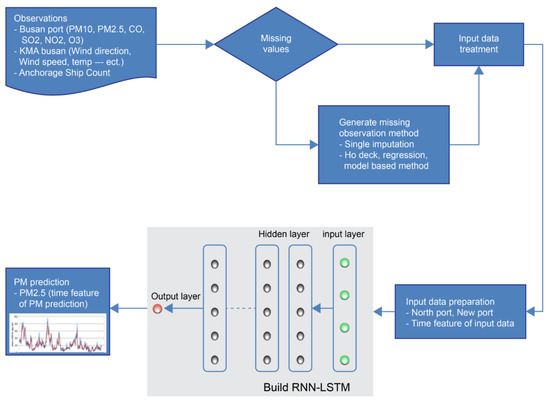
Figure 1.
Workflow for predicting the concentration of PM2.5 using the recurrent neural network and long short-term memory (RNN-LSTM) model.
Hidden nodes, hidden layers, and epoch methods were used to select the hyperparameters and improve the prediction performance. In addition, air quality was predicted only when air quality, meteorological, and shipping activity data were applied.
2.1. Monitoring Data
For air quality data, we used the monitoring data from Busan North Port and Busan New Port. For meteorological data, we used the monitoring data of the Busan Automated Synoptic Observing System (ASOS). The monitoring locations are shown in Figure 2. Monitoring in Busan North Port and Busan New Port began in November 2018. The learning period in this study was from 00:00 on 1 January 2019 to 23:00 on 31 January 2020. The predictions were performed from 00:00 on 1 February 2020 to 23:00 on 29 February 2020, and hourly data were employed.
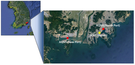
Figure 2.
Locations of Air Quality Monitoring System (AQMS) sites and the Korea Meteorological Administration (KMA) Automated Synoptic Observing System (ASOS) site in Busan Port.
Datasets were prepared for the air quality, meteorological data, and ship berths around Busan Port. Among the 13 data dimensions in Table 1, the 6 air pollutant items were collected from the monitoring points in Busan North Port and Busan New Port, the 5 meteorological items were collected from the Busan ASOS, and the berth information was collected from the Shipping Port Management Information System (PORT-MIS). At this time, the emission source of air pollutants is limited to ships, and the activity of the emission source is defined as the number of the anchored ships. The air quality, meteorological, and berth data for Busan North Port and New Port are summarized in Table 2.

Table 1.
Data types, variables, and units of input dataset of RNN-LSTM.
Table 2.
Summary of the PM2.5, shipping activity, and meteorological data statistics (time period: 1 January 2019 to 29 February 2020).
Missing values are an important issue in data processing. Most statistical methods have incomplete values. Missing value imputation is one of the methods used to create a complete dataset [24]. Missing value imputation methods include least squares imputation techniques, random data imputation, and hot deck, regression, and model-based methods [25,26,27].
Air quality and meteorological data were collected in real time. It is noteworthy to mention here the possibility for the generation of invalid data owing to equipment faults, maintenance, and quality assurance/quality control (QA/QC). In accordance with the method suggested by Hair et al. (2006), we processed our missing data using the smooth curve-fitting method [28] for cases with a missing data rate of less than 10.
Data standardization converts data to the same level in each data area and converts the map into specific intervals. It is used to create pure dimensionless quantities or values from data by removing the unit limitations in various data fields. Finally, index comparisons and weights can be generated for different units or scales. Here, we used the zero-mean standardization method, which is the most common standardization method in the raw data field, using the mean and standard deviation:
where z is the z-score, x is the observed value, μ is the mean, and σ is the standard deviation. The standardized data followed a standard normal distribution, with a mean value of 0 and a standard deviation of 1.
2.2. RNN-LSTM
2.2.1. Overview
The RNN can process long sequence data; however, its performance decreases with increased sequence length. This phenomenon is termed the long-term dependency problem. One of the variant RNN models used to overcome this problem is LSTM [29]. In this study, we employed the LSTM model, which recognizes patterns in time-series data.
The LSTM models were set up in four layers with a recursive structure. The core of the LSTM is the state of continuous cells that come in through the gate. The state of continuous cells is called a conveyor belt. The information that comes in on the conveyor belt is delivered without any change. The LSTM can add or delete information through the input gate, forget gate, and output gate. Thus, the gate selectively delivers information and continues to learn by removing the previous data. The mathematical formulas for the LSTM calculated using the LSTM gate vector are as follows:
where is a forget gate vector and serves as a weight that remembers the previous state of the cell, is an input gate vector that serves as a weight for acquiring new information, , in contrast, is an output gate vector that serves to select an output candidate, is an input vector, is an output vector, is a cell state vector, W is the weights matrix, and b is a bias vector. Importantly, , , and are the gate vectors. LSTM uses two types of activation functions— is a sigmoid function and tanh is a hyperbolic tangent function. Additionally, the dimension of is [t × m], the dimension of is [t × t], the dimension of input is [m × 1], the hidden node’s dimension is [t × 1], and the dimension of b is [t × 1]. W is initialized by the Xavier method. Bias vector b is initialized to 1 for the forget gate while all other biases are initialized to zero [29].
2.2.2. Implementation of RNN-LSTM
The RNN-LSTM was designed based on the algorithm presented in Table 3 and configuration settings in Table 4. The LSTM was composed of 13 input nodes of the air quality monitoring dataset, meteorological dataset, and hourly ship berths of Busan North Port and Busan New Port. As the ranges of the input data differed (i.e., application of the LSTM algorithm would be limited), data normalization was performed. After the data were standardized and used as a network layer, the sequence was returned. The algorithm specified the hidden node and hidden layer as variables, and the layer generated a single prediction for the results of these variables.
Table 3.
Algorithm of RNN-LSTM designed for data training and prediction.
Table 4.
Training data partition and hyperparameter settings for RNN-LSTM.
The prediction performance of the RNN-LSTM, and the potential to achieve optimal prediction performance, only varies by how the learning is repeated according to the hidden node and hidden layer set as variables in the algorithm [30]. The scenario for predicting air quality around Busan Port in the present study is presented in Table 3. The air pollutants emitted by ships are the result of the combustion of fuel oil. In general, ships are known to use a large amount of fuel oil regardless of their tonnage. However, ships that have a larger tonnage emit larger amounts of air pollutants because they use more fuel. Of the 8880 vessels operating in the waters near South Korea, 850 vessels accounted for more than 2000 tons (i.e., ~10% of the total tonnage of the ships). Therefore, in this study, we constructed a scenario in which we considered the number of berths of ships weighing 2000 tons or more, and the number of berths of all ships to clarify the influence of large ships. To determine the optimal prediction performance, among the parameters, Adam was selected for the optimizer, 100 for the batch size, 0.001 for the learning rate, and L2 Loss for the loss function.
For the learning conditions using RNN-LSTM, we used 27 learning methods, three hidden nodes (30, 60, 120), three hidden layers (1, 2, 3), and three epochs (10, 15, 20), which were incorporated in each case in Table 5 to predict the air quality that represented the highest performance.
Table 5.
Air quality prediction scenarios (learning and verification period: 1 January 2019 to 31 January 2020; prediction period: 1 February 2019 to 29 February 2020).
To evaluate the performance of the RNN-LSTM model, we employed four statistical methods, i.e., IOA, RMSE, normalized mean bias (NMB), and mean normalized gross error (MNGE) in the model and for the measurement values.
The IOA measures the agreement between the observed and predicted values, and IOA values range between 0 and 1. It is appropriate if the value is 0.5 or higher, and it is highly appropriate if the value is 1. The RMSE measures the degree of error dispersion for the observed values and the model prediction values. An RMSE value of 0 indicates a higher accuracy of the predicted value. The NMB measures the difference between the model and observed values in the observed spatial and temporal patterns. An NMB value close to 0 indicates that the model appropriately reflects the observed values. The MNGE is a relative error that represents the absolute error as a percentage of the true value. This determines the accuracy of the model [31,32,33,34].
Here, denotes the observed value, denotes the model prediction value, denotes the mean of the observed value, and denotes the time.
3. Results and Discussion
For the learning conditions, RNN-LSTM was employed in each case to predict the air quality that represents the highest performance. The air quality prediction results are presented in Table 6, and Figure 3 and Figure 4.
Table 6.
Statistical analysis of RNN-LSTM-modeled and AQMS-observed PM2.5 (Case 1, 4: AQMS + ASOS; Case 2, 5: AQMS + ASOS + all anchored ships; Case 3, 6: AQMS + ASOS + anchored ships over 2000 tons; Case 1~3: North Port; Case 4~6: New Port).
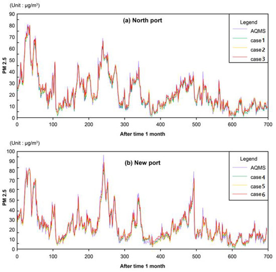
Figure 3.
Comparisons between the (a) North Port and (b) New Port RNN-LSTM-predicted and AQMS-observed PM2.5 (Case 1, 4: AQMS + ASOS; Case 2, 5: AQMS + ASOS + all anchored ships; Case 3, 6: AQMS + ASOS + anchored ships over 2000 tons).
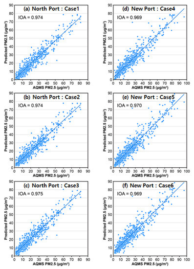
Figure 4.
Scatter plot of observation and prediction results for PM2.5. (a,d) AQMS + ASOS, (b,e) AQMS + ASOS + all anchored ships, (c,f) AQMS + ASOS + anchored ships over 2000 tons.
In Case 1, the IOA was 0.651–0.974, the RSMSE was 4.84–12.45 µg/m3, the NMB was −5.1–17.2%, and the MNGE was 22.59–80.06%. In Case 2, the IOA was 0.748–0.974, the RMSE was 4.82–12.05 µg/m3, the NMB was −9.2–21.1%, and the MNGE was 23.41–90.39%. In Case 3, the IOA was 0.762–0.975, the RMSE was 4.85–10.87 µg/m3, the NMB was −16.3–11.6%, and the MNGE was 23.16–59.93%. Among Cases 1 to 3 for predicting air quality in Busan North Port, Case 3 showed the highest prediction performance, in which air quality monitoring data, meteorological data, and data regarding the hourly berths of 2000 ton or larger ships were incorporated.
In Case 4, the IOA was 0.635–0.969, the RMSE was 5.87–13.86 µg/m3, the NMB was −5.9–8.2%, and the MNGE was 23.79–76.38%. In Case 5, the IOA was 0.682–0.970, the RMSE was 5.83–13.26 µg/m3, the NMB was −12.5–6.8%, and the MNGE was 24.97–68.68%. In Case 6, the IOA was 0.729–0.970, the RMSE was 5.82–12.72 µg/m3, the NMB was −9.6–8.9%, and the MNGE was 23.67–73.35%. Among Cases 1 to 6, where the PM2.5 concentrations were predicted for Busan New Port, Case 5 showed the IOA with the best prediction performance. In Busan New Port, along with air quality monitoring data and meteorological data, data regarding the hourly berths of ships anchored in Busan New Port were incorporated.
In Figure 3, the time series distributions of the observed data and predicted data of Busan North Port and Busan New Port cases indicate that the predicted values represent the trend of the observed values well. Figure 4 shows the IOA of the observed and predicted results. The IOA of Busan North Port was slightly higher than that of Busan New Port. In Busan North Port, Case 3 (AQMS + ASOS + berths of 2000 tons or larger ships) was used as input data. In Busan New Port, Case 5 (AQMS + ASOS + berths of all ships) was used as the input data. Hence, this result suggests that the method involving the incorporation of the activity of air pollutant emission sources can result in a higher prediction performance than the method involving predictions using air quality and meteorological data. In the future, the prediction performance could be improved upon by incorporating data regarding the activity of the ground support facilities of the air pollutant emission sources in the port.
The main research direction to date has been to utilize atmospheric observation data and meteorological data when predicting air quality through machine learning. Our research method applies machine learning methods that consider the activity of the emission source as well as atmospheric observation data and meteorological data. The prediction considering the activity of the emission source showed an IOA of 0.969 to 0.975. This shows that our proposed prediction method is better able to predict air quality.
At the inflection point of this study, there are various emission sources other than ships in the port, but there is a limit to considering the activity of these sources. In the future, if the prediction is made considering the activity of heavy trucks, it will be possible to help reduce the error and improve the prediction performance more efficiently.
4. Conclusions
In this study, we investigated a method for predicting the degree of air pollution in a port. We aimed to predict the air quality around Busan Port using RNN-LSTM. Previous studies employed a prediction method that uses only air quality and meteorological data as inputs. However, the extended method proposed in this study predicts air quality by incorporating data regarding emission sources that emit air pollutants (i.e., ship activities). Air quality monitoring network data for Busan North Port and Busan New Port were used to predict the air pollutants as a specific method for predicting air pollution, and the meteorological data of the Busan ASOS were also integrated and used. With respect to the activity input data of the emission sources, the hourly number of berths at the port was incorporated using the entry and exit times in the PORT-MIS. Statistical analysis methods, such as IOA, RMSE, NMB, and MNGE, were employed to evaluate the prediction performance. In the case of Busan North Port, where the air quality, weather, and the number of berths of ships 2000 tons or larger were analyzed, the results showed that the highest prediction performance was found at a maximum IOA of 0.975, RMSE of 4.88 µg/m3, NMB of 2.8%, and MNGE of 24.283. As expected, large ships have a greater impact on air pollution in Busan North Port. In the case of taking into consideration air quality, weather, and the number of berths of all ships in Busan New Port, the IOA was 0.970, the RMSE was 5.87 µg/m3, and the NMB between −0.9% and 25%. Busan New Port is still evolving. This conclusion was based on the geometrical conditions of the measurement network that were affected by all ships using the new port as well as large ships. Therefore, the extended method that employs ship activities as the emission source is advantageous, with a higher prediction performance than other existing methods.
In the future, we plan to study ways to reduce the dimension of input data in order to examine the major factors affecting air quality prediction. In addition, further research will be performed to improve predictive performance in consideration of emission sources other than ships, which are the major sources of emissions at ports. The methodology of this study can be applied to methods of predicting air quality around airports considering emission sources such as aircraft, or air quality in urban areas considering emission sources such as automobiles. Furthermore, it can be used to improve the performance of numerical models such as 3D CTM, which has limitations in predicting air pollution, by applying air pollutant emissions in real time.
Author Contributions
Conceptualization, H.H., H.J., C.Y. and H.K.; Methodology, H.H., H.J., C.Y. and H.K.; Supervision, C.Y. and H.K.; Writing—original draft, H.H. and H.J.; Writing—review and editing, C.Y. and H.K. All authors have read and agreed to the published version of the manuscript.
Funding
This research received no external funding.
Institutional Review Board Statement
Not applicable.
Informed Consent Statement
Not applicable.
Data Availability Statement
All data analyzed or generated during the study are included in the paper, and the data used for the study are displayed as URLs in the paper in detail on where the data can be found.
Acknowledgments
We appreciate the air quality index data provided by the Korean Ministry of Environment (http://www.airkorea.or.kr (accessed on 6 September 2021)).
Conflicts of Interest
The authors declare no conflict of interest.
References
- Moon, D.H.; Kwon, S.O.; Kim, S.Y.; Kim, W.J. Air pollution and incidence of lung cancer by histological type in Korean adults: A Korean national health insurance service health examinee cohort study. Int. J. Environ. Res. Public Health 2020, 17, 915. [Google Scholar] [CrossRef] [Green Version]
- Koenig, J.Q. Health Effects of Particulate Matter. In Health Effects of Ambient Air Pollution; Springer: Boston, MA, USA, 2000. [Google Scholar] [CrossRef]
- Wu, X.; Zhu, B.; Zhou, J.; Bi, Y.; Xu, S.; Zhou, B. The epidemiological trends in the burden of lung cancer attributable to PM2.5 exposure in China. BMC Public Health 2021, 21, 1–8. [Google Scholar] [CrossRef]
- WHO. WHO Air Quality Guidelines for Particulate Matter, Ozone, Nitrogen Dioxide and Sulfur Dioxide: Global Update 2005; World Health Organization: Geneva, Switzerland, 2005; pp. 1–21. [Google Scholar]
- Bailey, D.; Plenys, T.; Solomon, G.M.; Campbell, T.R.; Feuer, G.R.; Masters, J. Harboring Pollution Strategy to Clean Up U.S. Natural Resources Defense Council; Transportation Research Board: Washington, DC, USA, 2004; p. 85. [Google Scholar]
- Han, C.H. Air pollution reduction strategies of world major ports. Int. Commer. Law Rev. 2010, 48, 27–56. [Google Scholar]
- EPA. Current Methodologies in Preparing Mobile Source Port-Related Emission Inventories; ICF International: Fairfax, VA, USA, 2009. [Google Scholar]
- IMO. Guidelines for Consistent Implementation of the 0.50% Sulphur Limit under Marpol; International Maritime Organization: London, UK, 2020. [Google Scholar]
- Zamani Joharestani, M.; Cao, C.; Ni, X.; Bashir, B.; Talebiesfandarani, S. PM2.5 prediction based on random forest, XGBoost, and deep learning using multisource remote sensing data. Atmosphere 2019, 10, 373. [Google Scholar] [CrossRef] [Green Version]
- EPA. The Community Multiscale Air Quality (CMAQ) Developer Guide; United States Environmental Protection Agency: Washington, DC, USA, 2019.
- Schönig, S.; Jasinski, R.; Ackermann, L.; Jablonski, S. Deep Learning Process Prediction with Discrete and Continuous Data Features. In Proceedings of the 13th International Conference on Evaluation of Novel Approaches to Software Engineering, Funchal, Portugal, 23–24 March 2018; pp. 314–319. [Google Scholar] [CrossRef]
- Sherstinsky, A. Fundamentals of recurrent neural network (RNN) and long short-term memory (LSTM) network. Phys. D Nonlinear Phenom. 2020, 404, 132306. [Google Scholar] [CrossRef] [Green Version]
- Kalchbrenner, N.; Danihelka, I.; Graves, A. Grid long short-term memory. arXiv 2015, arXiv:1507.01526. [Google Scholar]
- Chung, J.; Kastner, K.; Dinh, L.; Goel, K.; Courville, A.; Bengio, Y. A recurrent latent variable model for sequential data. arXiv 2015, arXiv:1506.02216. [Google Scholar]
- Bayer, J.; Osendorfer, C. Learning stochastic recurrent networks. arXiv 2014, arXiv:1411.7610. [Google Scholar]
- Wu, Z.; Wu, X.; Wang, Y.; He, S. PM2.5/PM10 ratio prediction based on a long short-term memory neural network in Wuhan, China. Geosci. Model. Dev. 2020, 13, 1499–1511. [Google Scholar] [CrossRef] [Green Version]
- Xayasouk, T.; Lee, H.M.; Lee, G. Air pollution prediction using long short-term memory (LSTM) and deep autoencoder (DAE) models. Sustainability 2020, 12, 2570. [Google Scholar] [CrossRef] [Green Version]
- Chang, Y.; Chiao, H.; Abimannan, S.; Huang, Y.; Tsai, Y.; Lin, K. An LSTM-based aggregated model for air pollution forecasting. Atmos. Pollut. Res. 2020, 11, 1451–1463. [Google Scholar] [CrossRef]
- Kim, H.S.; Park, I.; Song, C.H.; Lee, K.; Yun, J.W.; Kim, H.K.; Jeon, M.; Lee, J.; Han, K.M. Development of a daily PM10 and PM2.5 prediction system using a deep long short-term memory neural network model. Atmos. Chem. Phys. 2019, 19, 12935–12951. [Google Scholar] [CrossRef] [Green Version]
- Russo, A.; Raischel, F.; Lind, P.G. Air quality prediction using optimal neural networks with stochastic variables. Atmos. Environ. 2013, 79, 822–830. [Google Scholar] [CrossRef] [Green Version]
- Zhou, Q.; Jiang, H.; Wang, J.; Zhou, J. A hybrid model for PM2.5 forecasting based on ensemble empirical mode decomposition and a general regression neural network. Sci. Total Environ. 2014, 496, 264–274. [Google Scholar] [CrossRef] [PubMed]
- Qi, Z.; Wang, T.; Song, G.; Hu, W.; Li, X.; Zhang, Z. Deep air learning: Interpolation, prediction, and feature analysis of fine-grained air quality. IEEE Trans. Knowl. Data Eng. 2017, 30, 2285–2297. [Google Scholar] [CrossRef] [Green Version]
- Zhao, J.; Deng, F.; Cai, Y.; Chen, J. Long short-term memory-fully connected (LSTM-FC) neural network for PM2.5 concentration prediction. Chemosphere 2019, 220, 486–492. [Google Scholar] [CrossRef]
- Audigier, V.; Husson, F.; Josse, J. A principal component method to impute missing values for mixed data. Adv. Data Anal. Classif. 2016, 10, 5–26. [Google Scholar] [CrossRef]
- Ilin, A.; Raiko, T. Practical approaches to principal component analysis in the presence of missing values. JMLR 2010, 11, 1957–2000. [Google Scholar]
- Rencher, A.C. Methods of Multivariate Analysis, 2nd ed.; John Wiley & Sons: New York, NY, USA, 2002. [Google Scholar]
- Hair, F. Multivariate Data Analysis: An Overview. In International Encyclopedia of Statistical Science; Lovric, M., Ed.; Springer: Berlin/Heidelberg, Germany, 2011; Volume 12, pp. 904–907. [Google Scholar]
- Akima, H. A New Method of Interpolation and Smooth Curve Fitting. J. ACM 1970, 17, 589–602. [Google Scholar] [CrossRef]
- Reddy, V.; Mohanty, S. Deep Air: Forecasting Air Pollution in Beijing, China. Environ. Sci. 2017. Available online: https://www.ischool.berkeley.edu/sites/default/files/sproject_attachments/deep-air-forecasting_final.pdf (accessed on 30 August 2021).
- Hochreiter, S. Long short-term memory. Neural. Comput. 1997, 9, 1735–1780. [Google Scholar] [CrossRef] [PubMed]
- Hogrefe, C.; Rao, S.T.; Kasibhatla, P.; Kallos, G.; Tremback, C.J.; Hao, W.; Olerud, D.; Xiu, A.; McHenry, J.; Alapaty, K. Evaluating the performance of regional-scale photochemical modeling systems: Part I—Meteorological predictions. Atmos. Environ. 2001, 35, 4159–4174. [Google Scholar] [CrossRef]
- Chang, L.; Scorgie, Y.; Duc, H.N.; Monk, K.; Fuchs, D.; Trieu, T. Major source contributions to ambient PM2.5 and exposures within the New South Wales Greater Metropolitan Region. Atmosphere 2019, 10, 138. [Google Scholar] [CrossRef] [Green Version]
- Tesche, W.; Mcnally, D.E.; Tremback, C. Operational Evaluation of the MM5 Meteorological Model over the Continental United States: Protocol for Annual and Episodic Evaluation; U.S. EPA: Washington, DC, USA, 2002; p. 51.
- Emery, C.; Tai, E.; Yarwood, G. Enhanced Meteorological Modeling and Performance Evaluation for Two Texas Ozone Episodes; ENVIRON International Corporation: Novato, CA, USA, 2001; Volume 31, p. 235. [Google Scholar]
Publisher’s Note: MDPI stays neutral with regard to jurisdictional claims in published maps and institutional affiliations. |
© 2021 by the authors. Licensee MDPI, Basel, Switzerland. This article is an open access article distributed under the terms and conditions of the Creative Commons Attribution (CC BY) license (https://creativecommons.org/licenses/by/4.0/).