The Impact of Climate Change on Urban Thermal Environment Dynamics

Abstract

The human population is increasing. The ongoing urbanization process, in conjunction with climate change, is causing larger environmental footprints. Consequently, quality of life in urban systems worldwide is under immense pressure. Here, the seasonal characteristics of Maribor’s urban thermal environment were studied from the perspectives of surface urban heat island (SUHI) and urban heat island (UHI) A remote sensing thermal imagery time series and in-situ measurements (stationary and mobile) were combined with select geospatial predictor variables to model this atmospheric phenomenon in its most intensive season (summer). Finally, CMIP6 climate change scenarios and models were considered, to predict future UHI intensity. Results indicate that Maribor’s UHI intensity maximum shifted from winter to spring and summer. The implemented generalized additive model (GAM) underestimates UHI intensity in some built-up parts of the study area and overestimates UHI intensity in green vegetated areas. However, by the end of the century, UHI magnitude could increase by more than 60% in the southern industrial part of the city. Such studies are of particular concern, in regards to the increasing frequency of heat waves due to climate change, which further increases the (already present) heat stress in cities across the globe.

1. Introduction

Nowadays, cities are the dominant habitats of the human species. In 2000, about 47% of people lived in urban systems [1]. This proportion increased to 55% by 2018 and could reach 60% by 2030 [1]. By then, it is expected that 44% of the world’s population will live in cities of at least half a million inhabitants [1]. With urban area expansion, artificial materials (concrete, asphalt, tiles, metals etc.) replace natural vegetation [2]. Urban construction thus causes a change in surface albedo, emissivity, and heat capacity [3]. As a result, a net influx of heat into the urban atmosphere is detectable [4], which is further potentiated by anthropogenic activities [5] in which heat is released (heating, industry, and transport) [6]. This evident positive air temperature anomaly between urban and rural areas is the urban heat island (UHI) [7]. UHI is considered one of the most problematic consequences of rapid urbanization [7]. It can cause health issues [5] and decrease productivity [8], especially during increasingly frequent, climate change-related heat wave events [9].

To measure and evaluate UHI intensity, two methodological approaches prevail. Larger metropolitan areas and mid-size cities require thermal remote sensing data and, thus, cloudless meteorological conditions, in order to study the surface urban heat island (SUHI), which is a land surface temperature (LST) derivate [10,11,12,13]. In smaller cities, seasonal- and weather-independent “in-situ” air temperature measurements (stationary or mobile) can be applied, which is a major advantage [14,15,16]. However, the annual (seasonal) UHI intensity regime and the surface urban heat island (SUHI) have been the subjects of several previous studies. From the SUHI perspective, Bechtel et al. [17] found that, in some US coastal cities (San Francisco, Los Angeles, and San Diego), the highest SUHI intensity can be expected in the spring months and the lowest in late summer, while in cities such as Fresno and Sacramento, SUHI intensity peaks in September and October. In contrast, cities in semi-arid environments (Phoenix) actually experience, in summer and fall, lower surface temperatures than the surrounding countryside owing to irrigation (the urban cold island phenomenon). Pongrácz et al. [18] studied surface thermal properties of several European cities (Munich, Milan, Warsaw, and Budapest) and concluded that the most intense SUHIs develop during the day in the summer (June and July). From the UHI perspective, Zhou et al. [19] reported that London’s UHI intensity peaks around the summer solstice, while the highest temperatures in the city are usually reached in late July and early August. The same UHI intensity seasonal pattern was observed in Kumagaya city (Japan), but with significantly higher temperature differences at night [20].

All these findings prove that urban system thermal environments are complex, dynamic, and unique. However, there is still a lack of studies considering future climate change conditions on the UHI phenomenon. We sought to bridge this gap and, thus, linked the two methodological procedures (UHI and SUHI) with the currently available CMIP6 climate change scenarios and global climate models, to predict UHI intensity in the second largest city in Slovenia (Maribor). More precisely, we addressed the following research questions: (a) how dynamic is the UHI phenomenon in Maribor from the seasonal perspective, and did it change? (b) Can geospatial predictors explain Maribor’s summer UHI intensity pattern? Finally, (c) will climate change affect UHI intensity in small urban systems with dispersed green areas and water bodies?

2. Materials and Methods

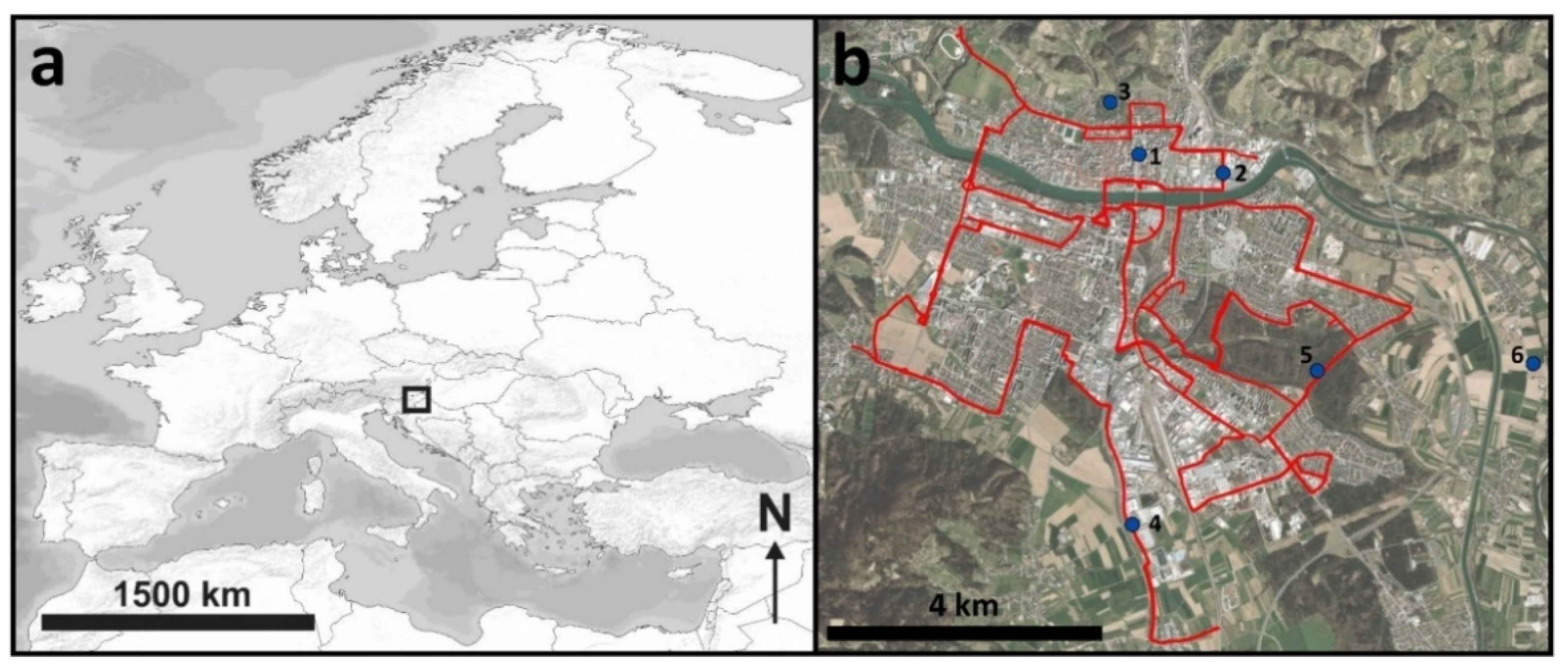
2.1. Study Area

Maribor lies at the conjunction of the pre-Alpine and Pannonian areas of northeastern Slovenia (Figure 1a), along the river Drava. The city, with 95.767 inhabitants today [21], flourished in the middle of the 19th century, when the first industrial plants were built in connection with the construction of the railway network program between Vienna (AUT) and Trieste (ITA). Soon, other industries began to develop, but experienced a decline after the breakup of Yugoslavia in 1991. Today, Maribor is attempting to create its identity in the service economic sector and as a university center for northeastern Slovenia. The city has experienced accelerated population growth and spatial development since the 1960s, mainly owing to intensive rural immigration. The built-up part spread to the south, west, and east, occupying former farmland. Today, several parks (Mestni park, Trg Borisa Kidriča, Slomškov trg, Magdalenski park) and two forest areas (Stražun and Betnavski gozd) are still preserved (Figure 1b). Moreover, the river Drava divides Maribor into two parts, with a riverbed up to 160 m wide; it is thus an important local climate modifier [22].

2.2. Seasonal SUHI Characteristics

Surface thermal properties are among the main contributors to the UHI phenomenon. In order to capture seasonal Land Surface Temperature (LST) variability in the study area, 22 LANDSAT 8 cloud free satellite images (5 in winter (December, January, February), spring (March, April, May), and summer (June, July, August), and 7 in autumn (September, October, November)) between 2013 and 2020 were obtained from the EarthExplorer web platform [23] (path = 190, row = 28; scene center time between 10 and 10:25 am GTM). Both thermal channels (band 10 and 11) were initially converted to at-satellite brightness temperature (in °C) by applying TerrSet2020’s Landsat algorithm [24] and were later averaged. Seasonal mean values of the resulting LST variable were calculated in the next step. Finally, we were able to estimate SUHI intensity according to the land use/land cover categories of the Urban Atlas (UA) 2018 database, provided by the Copernicus web platform [25]. The category Pastures (code 23000) served as the reference.

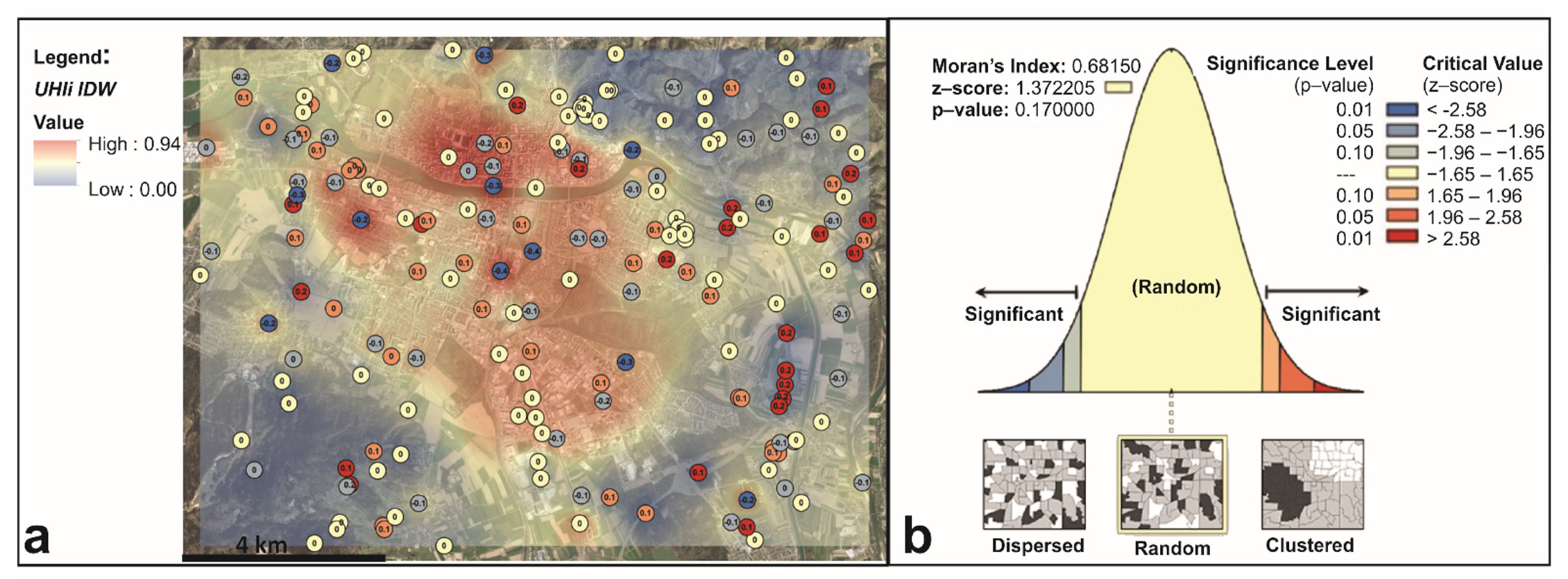
2.3. Seasonal UHI Characteristics

These two datasets (SUHI intensity and UA) were the basis for placing 6 HOBO MX2302A temperature and moisture loggers (accuracy = +/− 0.2 °C and +/− 2.5% RH), in Davis radiation shields, in different local climate zones [26] of the city. We covered 4 UA categories (arable land (1), forests (1), green urban areas (1) and industrial, commercial, public, military, and private units (3, considering the build-up area gradient)) (Figure 1b). All sensors were installed at 3 m height on an azimuth of 180° after preliminary testing of possible differences concerning the standard meteorological measurement height (2 m). A key reason for choosing a non-standard height was protection against vandalism. Air temperature and relative humidity data were recorded at half-hour intervals. The measurements began on 10 September, 2019. Thus, this study considers 659 measurement days and all four seasons (spring, summer, autumn, and winter). Fixed loggers provided at-point thermal boundary layer atmospheric conditions in different parts (local climate zones) of the city, but we were still lacking spatial information about the UHI phenomenon. To bridge this gap, mobile air temperature measurements were performed in summer 2020 and 2021, with an IoT MF-300 temperature datalogger (GPS position accuracy = +/− 2 m; GPS velocity accuracy = 0.1 m/s; GPS center frequency = 1575 +/− 3 MHz; temperature accuracy = +/− 0.3 °C; temperature resolution = 0.1 °C; acquired at www.pileus.si, accessed on 1 September, 2019). Its –165 dBm tracking sensitivity extends positioning coverage into places such as urban canyons and dense foliage environments, where GPS usage was not previously possible. The datalogger’s air temperature sensor was installed on a vehicle radio antenna (50 cm high) and was additionally protected with a small Davis radiation shield. Data were recorded each second (Figure 1b). Because of the road network structure, at certain points, such as road traffic lights, air temperature measurements were repeated. To filter out this noise (repeated air temperature records), a Python-based software was developed, which considered the exact time of the measurement and its direct spatial vicinity. Thus, other data errors were removed as well. Moreover, we measured air temperature differences, based on our stationary measurements approximately at the time when they reached the maximum value above urban structure (16:00 local time; started at 15:30, and finished at 17:00). Consequently, the mobile measurement time interval did not disrupt the results since differences in temperature records between the start and end of the measurement were statistically insignificant and, thus, ignored in further analysis. Because only temperature differences were analyzed, the ventilation effect (and traffic load) due to car movement (average speed = 40 km/h) was also disregarded. Altogether, 22 summer measurement days (90.444 air temperature records) were analyzed in different weather conditions/types (anti-cyclonic, cyclonic, and advective).

2.4. UHI Modeling

These mobile air temperature difference measurements enabled the development of the dependent variable summer UHI intensity (UHIi) in Maribor. To do so, a 300 m grid was designed in the ArcGIS environment [27] and laid over the entire study area. Next, the average air temperature for each quadrate/polygon covering the measuring route was calculated. Quadrates/polygons with less than 30 air temperature records were ignored. The Zonal statistics algorithm then enabled air temperature data extrapolation to UA categories. UHIi was calculated by subtracting the mean temperature value of the Pastures category (code 23000) from all other categories (as in the case of SUHI intensity). Finally, 10 random points per UA category (190 in total) were generated to operate with the point data, properly fit predictive models, and evaluate potential climate change impacts on Maribor UHI intensity.

To explain and model the detected UHIi geospatial pattern, the predictor variables per UA category were then produced: summer SUHI intensity (SUHIi), southness (= sinAspect) (sness), summer NDVI (NDVI), distance to water bodies (d2wb), building volume (bv), high vegetation volume (hvegv), and summer daily mean air temperature (June, July, August) (tas_summer). The predictor SUHIi was designed in the initial step as the product of LADSAT-based LST in reference to the Pastures category of the UA. The explanatory variable sness (a linearized form of the aspect variable where azimuth values are transformed into an index reaching values between −1 (northern slopes) and 1 (southern slopes)) was calculated in the ArcGIS environment from a LIDAR-based digital terrain model with a 1 m horizontal resolution, provided by the Slovenian Environmental Agency, which operates under the Ministry of the Environment and Spatial Planning [28]. Mean NDVI values per UA category were obtained by processing (Band 8—Band 4/Band8 + Band4) a Sentinel 2A satellite image (8 August, 2020) gathered from the Copernicus Open Access Hub [29]. Water bodies were extracted from the national land use database, which is freely available on the web platform owned by the Ministry of Agriculture, Forestry, and Food [30]. To transform this categorical variable, the Euclidean distance algorithm was applied in the ArcGIS environment [27]. Two databases were used to prepare the bv predictor. The above-mentioned LIDAR point cloud and the National register of buildings (a digital vector database), provided by the Ministry of Infrastructure and Spatial Planning [31]. A normalized digital surface model (nDSM) was calculated by considering the difference between first and ground returns. The National register of buildings was then used to calculate building volume per UA category. A similar approach was used to calculate high vegetation (tree) volume (hvegv). Vegetation cover was determined with NDVI and additionally validated with LIDAR cloud data classification (low, medium, or high vegetation). The tas summer predictor was developed for four time windows (current (1981–2011), 2011–2040, 2041–2070 and 2071–2100), two climate change scenarios (ssp370 (level of forcing = 7.0 W/m² in 2100) and ssp585 (level of forcing = 8.5 W/m² in 2100)) and five global climate models (GCMs) (GFDL-ESM4, IPSL-CM6A-LR, MPI-ESM1-2-HR, MRI-ESM2-0, UKESM1-0-LL), as provided by the CHELSA V2—CMIP6 database (spatial resolution = 30 arc seconds) [32]. To simplify modeling procedures, we used the tas_summer ensemble mean value from five models per future time window.

These predictors were finally checked for possible multicollinearity (Pearson’s correlation coefficient > 0.5 or < −0.5) and later used to model Maribor’s summer UHI intensity in current and future climate conditions. A generalized additive model (GAM) [33,34,35,36] was calibrated in the R statistical environment [37] by applying the mgcv package [38]. GAMs provide a structure for generalizing a general linear model by allowing additivity of non-linear functions of the variables [39]. The advantage of GAM is to limit the error in prediction of a dependent variable from various distributions by assessing unspecific functions, which are connected by means of a link function with the dependent variable [40]. Thus, our GAM model adequacy was tested with a generalized linear model (GLM) algorithm with the same predictors and designed with the Rcmdr package [41]. However, to additionally assure GAM model quality, its standardized residuals (over- and under-predictions) were tested for normal distribution and spatial autocorrelation (Moran’s I) in the ArcGIS environment [27]. After properly specifying the GAM model, the predict function within the mgcv package enabled future UHIi estimation by considering GCMs-based tas_summer values in time windows 2011–2040, 2041–2070, and 2071–2100, and emission scenarios ssp370 and ssp585.

2.5. Modeling Limitations

Since we sought to evaluate how future thermal conditions could influence the existing summer UHI pattern in Maribor, only the tas_summer variable was changed in the future climate change scenarios being considered. Of course, other UHI predictors will substantially change in the future and could alter the existing spatial pattern either positively or negatively. Higher air temperatures could potentially even decrease UHI intensity, especially in colder conditions (winter, spring, autumn). However, land use [42,43,44] and surface spectral change studies [45], as well as demographic trends [44,46] provided evidence that Maribor’s urban structure will not be particularly dynamic in the future. This fact excuses our consideration of all remaining UHI intensity predictors (bv, d2wb, NDVI, sness, SUHIi, hvegv) as temporarily stable. Moreover, we decided to use such an approach to illustrate possible outcomes in the current city structure if no climate change adaptation and mitigation actions are implemented. In order to improve the climate change-related UHI pattern change estimation, city development plans should be integrated. This information could be used to prepare future estimates for several of these UHI predictors (i.e., bv, d2wb, NDVI, and hvegv) and, thus, produce even more accurate results.

3. Results

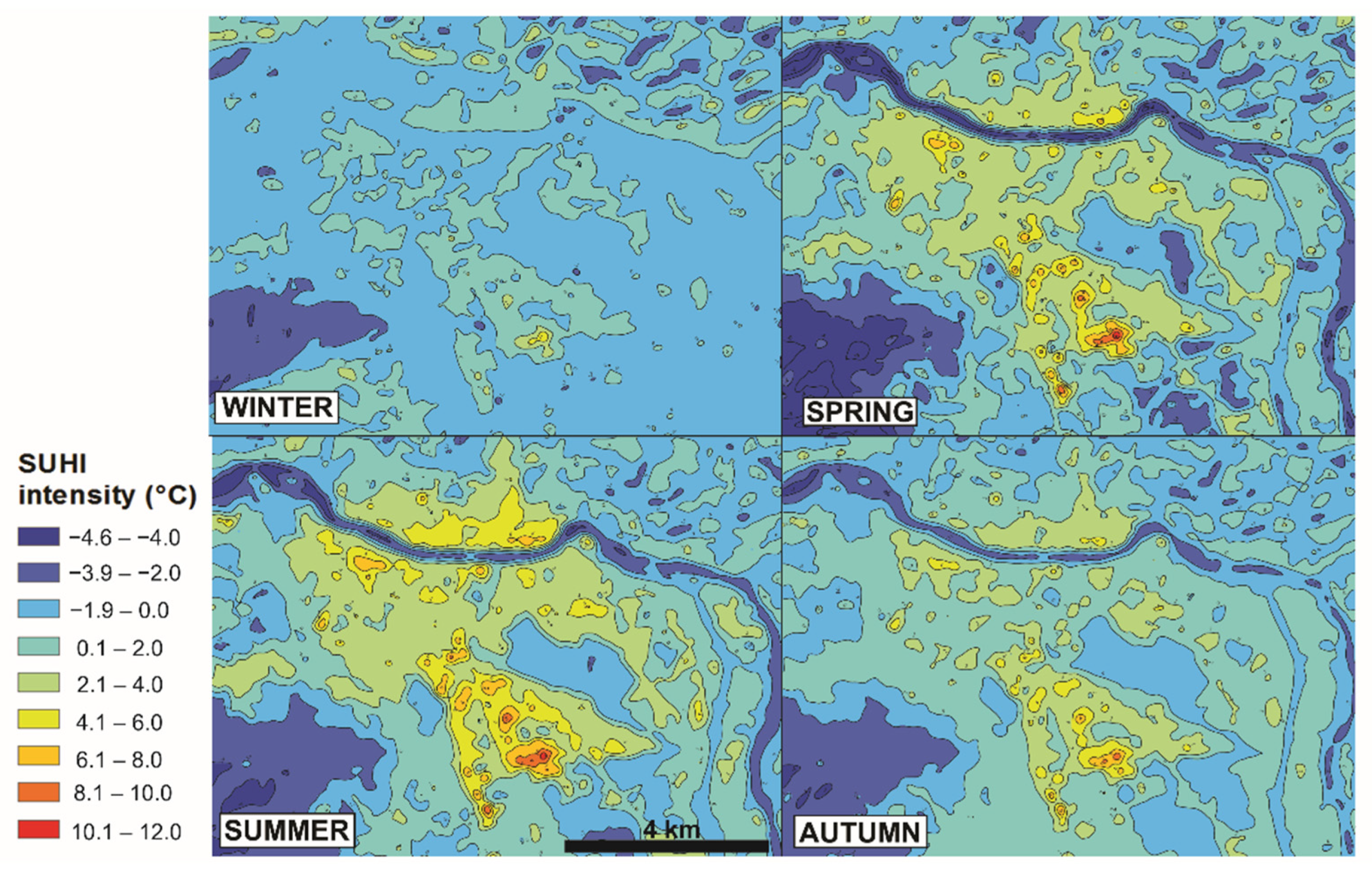
3.1. The Seasonal SUHI Intensity Footprint

The spatiotemporal analysis of the LST variable revealed that Maribor’s SUHI intensity pattern was most homogeneous and least pronounced in winter (Figure 2). The Tezno industrial zone in the SE part of the city and the southern-exposed surroundings occupied by vineyards (Mariborske gorice) on the northern built-up edge, stand out from the reference areas. Temperature differences between other land use categories were smaller (Figure 3). In spring, the SUHI intensity footprint increases and diversifies. Positive surface temperature anomalies were evident in the industrial zones of Tezno (SE part) and Melje (E part), in Studenci (W part), and in the shopping center area with associated parking lots. Negative deviations were observed along the river Drava and the corresponding hydroelectric canal, and in all closed forest areas (Stražun (E part), Betnavski gozd (S part), and Limbuška Dobrava (W part)). All of the smaller hot spots that had been identified in the spring were amalgamated in the summer. SUHI intensity increased up to 12 °C. All three industrial areas and the medieval center generated high levels of summer heat stress. Fortunately, the river Drava and other green urban areas create a large surface temperature contrast and, thus, break down the otherwise uniform SUHI footprint. In autumn, SUHI intensity decreases and simplifies. The spatial pattern is similar to that formed in spring.

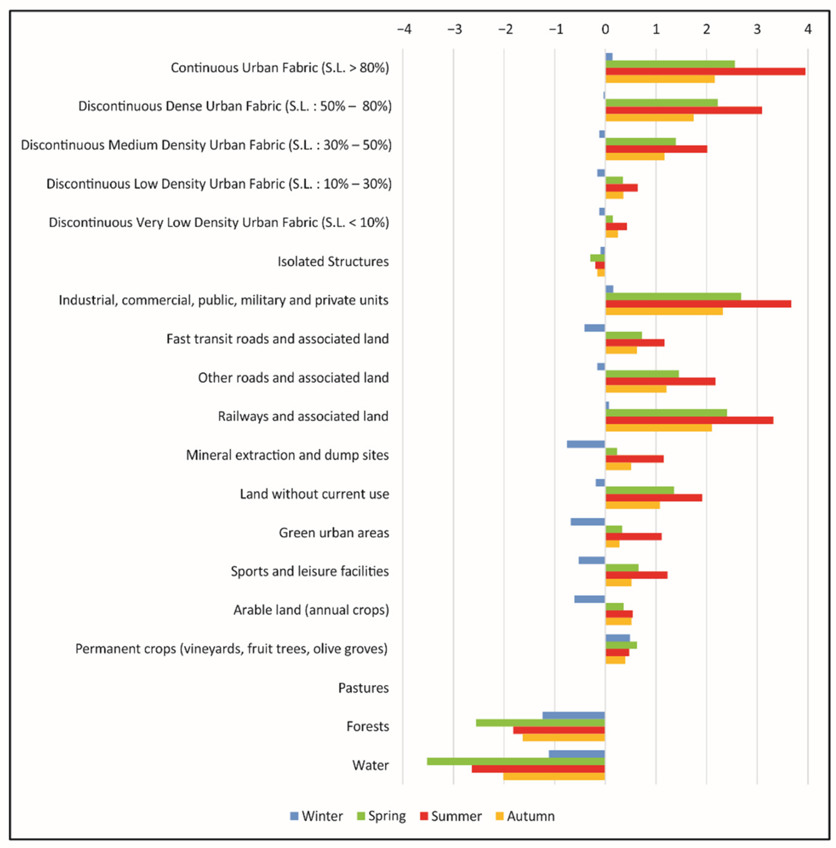
3.2. SUHI Intensity and Land Use

In the summer, the highest surface temperature differences compared to the reference UA category (pastures) occurred on continuous urban fabric areas (sealing level (SL) > 80%) (by 4.0 °C), on industrial, commercial, public, and military surfaces (by 3.7 °C), on railways, and associated land (by 3.3 °C) (Figure 3). Surface temperatures were lower on water surfaces (by 2.6 °C), in forest areas (by 1.8 °C), and for isolated structures (by 0.2 °C). A similar, but less intensive, pattern was observed in the spring and autumn. In winter, the highest positive deviations in LST occurred in the category permanent crops (represented mainly by vineyards) (by 0.5 °C). These are located on the steep southern slopes in the hilly surroundings of the city (Mariborske gorice). In contrast, forest areas, water bodies, arable land, and green urban areas were significantly cooler than pastures in winter.

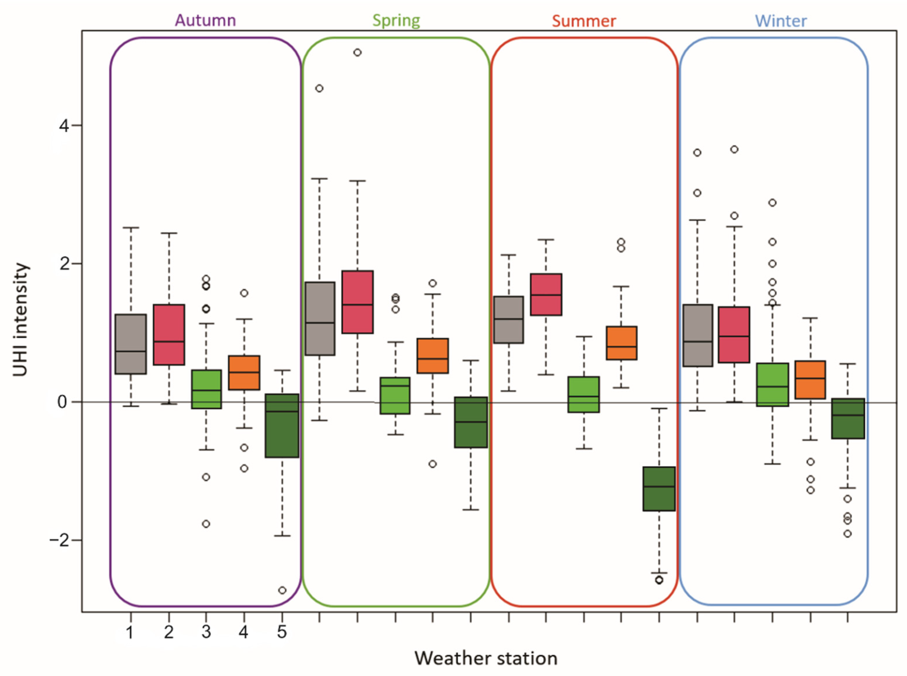
3.3. UHI Seasonal Dynamics

Remotely sensed data revealed the seasonal surface thermal pattern of the study area. Based on these findings, atmospheric thermal conditions were captured in different local climate zones (four UA categories (arable land, forests, green urban areas and industrial, commercial, public, military, and private units)). Figure 4 summarizes the seasonal development of the UHI phenomenon in Maribor. The two-way ANOVA analysis and the corresponding Tukey post-hoc test (p < α; α = 0.05) additionally confirmed significant differences in UHI intensity between seasons and UA categories (local climate zones). However, the largest differences in daily mean air temperature were evident in summer. The Stražun forest was clearly cooler than the reference surface (arable land in the city background), followed by the Mestni park green urban area, which was occasionally even hotter. Instead, all three built-up surfaces (the Melje industrial zone, the medieval city center, and the Tezno industrial zone) were significantly hotter than the rural surroundings. The same pattern was observed throughout the year, in spring and summer, with UHI intensity extremes occurring mainly in spring.

3.4. The Summer UHI Model

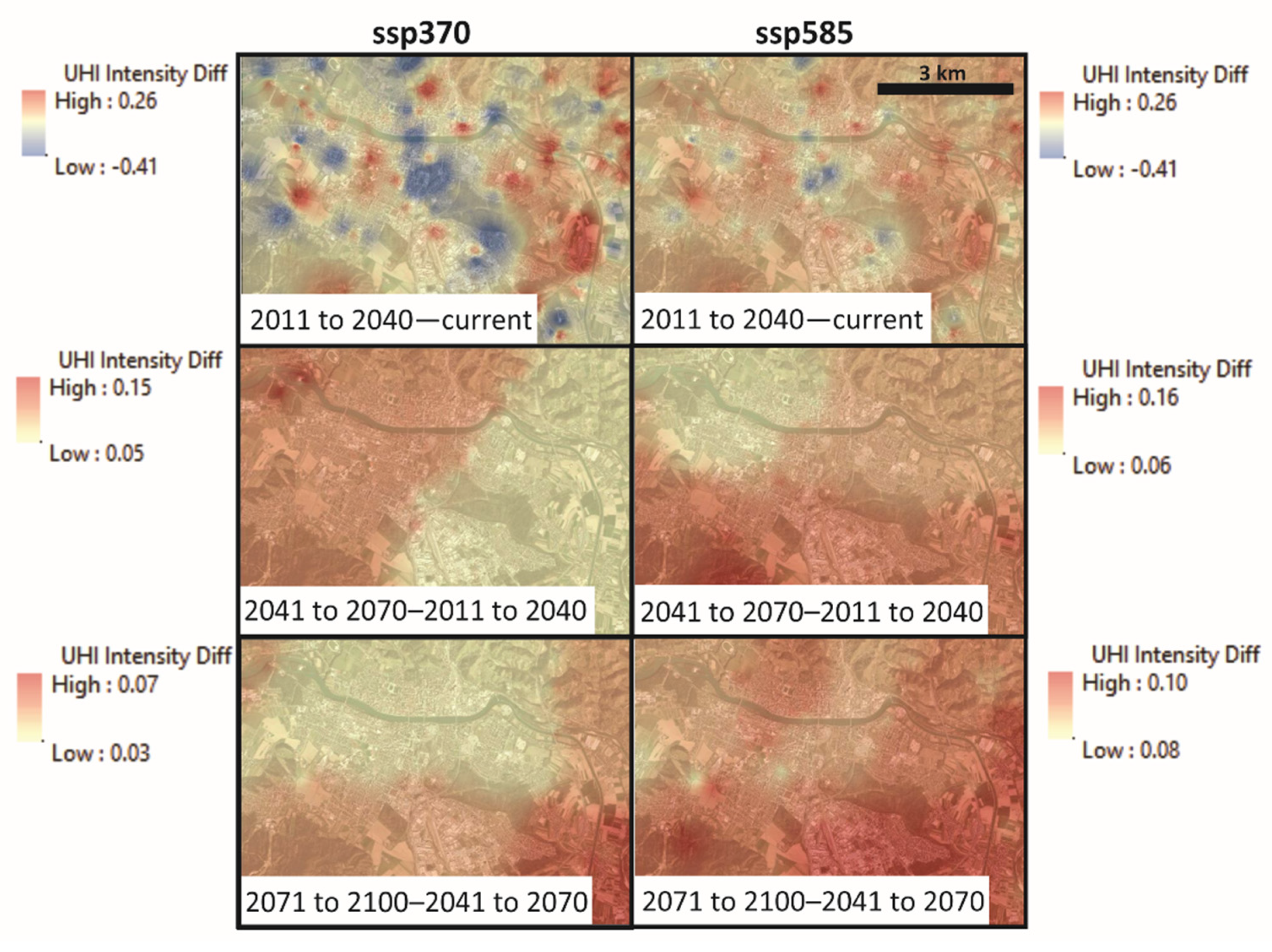
Both the perspectives on Maribor’s thermal environment (SUHI and UHI) indicated that citizens were exposed to extreme heat stress, particularly in summer. Thus, the focus of the research was turned to the summer season UHI. A GAM predictive model was designed by considering several explanatory variables known for their impacts (linear or non-linear) on the UHI phenomenon.

Table 1. Predictor variable correlation matrix (Pearson’s correlation coefficients).

Variable	bv	d2wb	NDVI	sness	SUHIi	tas_summer	hvegv
bv	1	0.13	−0.26	0.01	0.4	0.09	0.32
d2wb	0.13	1	0.22	0.12	0.3	−0.11	0.12
NDVI	−0.26	0.22	1	0.36	−0.3	−0.39	−0.03
sness	0.01	0.12	0.36	1	0.25	−0.08	0.02
SUHIi	0.4	0.3	−0.3	0.25	1	0.42	0.11
tas_summer	0.09	−0.11	−0.39	−0.08	0.42	1	0.08
hvegv	0.32	0.12	−0.03	0.02	0.11	0.08	1

shows that all the given predictors met the basic criteria, since correlation coefficients were within the −0.5 and +0.5 margin. However, low variance inflation factors (VIF < 3) additionally excused further use of these predictors in the modeling procedure.

The GAM approach fitted with seven predictor variables yielded 82.4% of explained deviance (

Table 2. GAM summary table.

Model: UHIi ~ s(SUHIi) + s(sness) + s(NDVI) + s(d2wb) + s(bv) + s(hvegv) +s(tas_summer) Parametric coefficients:
	Estimate	Std. Error	tvalue	Pr (>|t|)
(Intercept)	0.356884	0.008359	42.7	<2 × 10−16 ***
Approximate significance of smooth terms:
	edf	Ref. df	F	p-value
s(SUHIi)	5.547	6.736	29.566	<2 × 10−16 ***
s(sness)	7.782	8.545	3.938	<2 × 10−16 ***
s(NDVI)	7.029	7.855	7.058	<2 × 10−16 ***
s(d2wb)	2.506	3.123	5.863	0.000707 ***
s(bv)	1	1	18.101	0.0000356 ***
s(hvegv)	3.301	3.703	20.386	<2 × 10−16 ***
s(tas_summer)	1	1	0.661	0.41751
R-sq. (adj) = 0.793 Deviance explained = 82.4% V = 0.015682 Scale est. = 0.013275 n = 190

Significance codes: < 0.0001 ‘***’.

). All predictors, except tas_summer, had a statistically significant impact (p < α; α = 0.05) on the summer UHIi pattern. However, we kept the tas_summer predictor in the model, since it described current (and in predict mode, future) summer daily mean air temperatures in the study area. Four predictors (SUHIi, sness, NDVI, and d2wb) were non-linearly related to the dependent variable (edf > 1). The scale estimate (residual standard error squared = 0.013) indicated good predictive power for the designed UHIi GAM model.

Nonetheless, we additionally tested its quality by comparing it against a GLM approach, which assumes that all explanatory variables are linearly related with the given dependent variable (

Table 3. Analysis of Deviance summary.

Model 1: UHIi ~ SUHIi + sness + NDVI + d2wb + bv + hvegv + tas_summer Model 2: UHIi ~ s(SUHIi) + s(sness) + s(NDVI) + s(d2wb) + s(bv) + s(hvegv) + s(tas_summer)
	Residual	Df	Residual Deviance	Df Deviance	Pr (>Chi)
Model 1	182	5.8691
Model 2	160.83	2.135	21.166	3.734	<2.2 × 10−16 ***

Significance codes: < 0.0001 ‘***’.

). The analysis of deviance, based on χ² statistics, revealed that Maribor’s UHIi can be better modeled by applying a GAM (p < α; α = 0.05). However, before reaching any conclusions, standardized residuals were tested for possible spatial autocorrelation. The insignificant Moran’s I index (p > α; α = 0.05) proved that model over- and under-predictions were normally distributed and free of spatial autocorrelation (Figure 5). In other words, the model was properly specified without missing predictor variables. Moreover, Figure 5 indicates that major over-predictions are linked to the rural surroundings of the city, whereas under-predictions relate to the urban structure.

Finally, the developed GAM, the predict function in the mgcv package and the prepared climate scenario tas_summer predictor enabled future UHIi estimation in Maribor. Figure 6 illustrates the potential difference in UHIi concerning global emission scenarios ssp370 and ssp585. The four time windows under consideration (current (1981–2010), 2011–2040, 2041–2070, and 2071–2100) indicate a gradual increase in UHIi. Some possible improvements in summer UHIi are predicted only in the first half of the century (mainly under ssp370 conditions). The second half could potentially bring up to a 60% (>0.5 °C) UHIi increase, in particular in the southern industrial part of the city. However, differences between emission scenarios are evident (Figure 6).

4. Discussion

Ensuring high quality of life in urban systems is becoming increasingly difficult. In the last half of the century, the share of urban population has risen from 34% to 54%, and it is expected to reach 66% by 2050 [47]. In addition, cities worldwide are, owing to climate change, already exposed to higher mean air temperatures, changed precipitation patterns, and more frequent extreme weather events [48,49]). In NE Slovenia, where Maribor is located, air temperatures rose between 0.33 and 0.44 °C per decade (period 1961–2016) and in the summer months, between 0.44 and 0.59 °C per decade [50,51]). There, heat wave frequency has more than tripled since the 1960s [22]. Moreover, heat wave events are lasting longer (8.8 days more since 1990) and reaching higher maximum temperatures (up to 40.6 in 2013). However, urban warming is a manifestation of the direct (sensible heat) and indirect (land-cover transformation, climate change) alteration of the energy budget in the urban boundary layer [4,52,53]. These facts lead to the conclusion that a consequent intensification in the UHI effect is inevitable, in large agglomerations or small cities/towns, if no preventive or adaptation actions are implemented. From that perspective, studies like this, which provide applicative spatial prediction models, and which could roughly estimate the potential change in UHI intensity owing to direct or indirect urban system alterations, are of high importance.

However, the annual or seasonal dynamics of the UHI phenomenon in small cities/towns under climate change scenarios is, in general, poorly studied. We sought to bridge this gap and, thus, broke down Maribor’s thermal environment into individual entities that cause the current spatial UHI pattern, and will potentially co-create its thermal footprint in the second half of the 21st century. A time series of multispectral satellite imagery, along with stationary and mobile air temperature measurements, provided the first important discovery: the UHI intensity maximum in Maribor shifted, owing to climate change, from winter to spring and summer. Several urban climate scientists across the globe [4]) agreed that the UHI phenomenon in mid-latitude cities/towns is usually more pronounced in winter, moments before sunrise (longer nights provide more time for cooling and intensive house heating causes higher maximum air temperatures). The applied GAM summer UHI intensity model based on seven spatial predictor variables yielded good results. It should be emphasized that we tried to model Maribor’s summer UHI intensity with a multiscale geographically weighted regression (MGWR) [54], alongside the above-mentioned GLM. It yielded slightly better results (adjusted R2 = 0.84 and smaller over- and under- predictions), but we decided to calibrate a GAM because local regression models are still case-specific and cannot easily be transferred elsewhere in the geographical space [15,55]. Thus, our second important finding is that major over-predictions are linked to the rural surroundings of the city, whereas under-predictions exist in relation to the urban structure. In other words, the GAM model underestimates UHI intensity in some built-up parts of the study area and overestimates UHI intensity in green vegetated areas. Future UHI intensity scenarios could thus potentially be even worse. However, it should be emphasized that our predictions are made under the assumption that the city structure (predictor variables bv, d2wb, NDVI, sness, SUHIi, hvegv) remains temporarily stable. In other words, the uncertainty level of our predictions increases as soon as land use changes are applied. Other important summer UHI intensity modifiers that are not under consideration could decrease the proposed GAM model predictive power as well. For instance, a changed summer rainfall pattern could affect water bodies, vegetation (NDVI), and wind speed. As already mentioned, rising air temperatures alone could also decrease UHI intensity, especially in colder conditions (winter, spring, autumn). Studies about future bioclimatic conditions in the NE part of Slovenia (where Maribor is located) indicated that this region could potentially face hotter and dryer future climate conditions [56,57]. From that perspective, our results remain highly applicable despite the outlined weaknesses. Nonetheless, the third finding is that our methodology can be transferred to other cities across the globe, since it exploits statistical relations over all the data in the region of interest, and can therefore be applied even beyond the geographical limits of the measurements in cases where the physical settings remain similar. Finally, the new CMIP6 high-resolution climate change scenarios [32] indicate that Maribor could soon face a reasonable increase in summer UHI intensity, in particular in the southern industrial zone. By the end of the century, summer UHI magnitude in this area could increase by more than 60%. From that perspective, the last important message of this study is as follows: climate change preventive actions in urban systems are urgently needed to mitigate high levels of heat stress and assure a quality living environment for all social groups of citizens. Predictions for Maribor, which has several green urban areas and a large water body (the river Drava), are not optimistic. This is even more alarming for other Slovenian urban settlements, which are for historical reasons [58], much more concentrated.

Climate change and the UHI phenomenon are linked through a two-way interaction. First, global warming will increase UHI intensity in urban systems. Second, cooling strategies to reduce UHI intensity can help communities adapt to the impact of climate change, while also lowering the greenhouse gas emissions that cause climate change [59]. Most efforts to cool UHIs produce many benefits, including lower temperatures, greenhouse gases, air pollution, harmful health impacts, and electricity demand [60,61,62]. Efforts to reduce elevated temperatures in urban systems thus also help to address climate change and improve air quality. Moreover, such measures can help citizens become more resilient to some of the damaging impacts of modern climate change. Properly located green areas and water bodies represent good examples for urban cooling [63,64,65,66]. In this way, the need for fossil fuel-based transport (which is still dominant) to cooler parts of the city is reduced. In order to decrease the record-breaking CO₂ emissions (417 ppm, accessed on 17 June, 2021) [67] and somehow mitigate the impact of climate change at the global level, several multifaceted mitigation and adaptation measures must be taken as soon as possible. Starting with UHI mitigation strategies in densely populated areas is certainly a prime target, since countermeasures would, thus, be implemented precisely at the source of the greenhouse gas emissions.

References

1. United Nations. Available online: https://population.un.org/wup/Download/ (accessed on 15 February 2021).
2. Wang, W.; Liu, K.; Tang, R.; Wang, S. Remote sensing image-based analysis of the urban heat island effect in Shenzhen, China. Phys. Chem. Earth 2019, 168–175. [Google Scholar] [CrossRef]
3. Rizwan, A.M.; Dennis, L.Y.; Liu, C. A review on the generation, determination and mitigation of urban heat Island. J. Environ. Sci. 2008, 120–128. [Google Scholar] [CrossRef]
4. Hinkel, K.M.; Nelson, F.E.; Klene, A.E.; Bell, J.H. The urban heat island in winter at Barrow. Int. J. Climatol. 2003, 23, 1889–1905. [Google Scholar] [CrossRef] [Green Version]
5. Yang, L.; Qian, F.; Song, D.-X.; Zheng, K.-J. Research on urban heat-island effect. Procedia Eng. 2016, 11–18. [Google Scholar] [CrossRef]
6. Tam, B.Y.; Gough, W.A.; Mohsin, T. The impact of urbanization and the urban heat island effect on day to day temperature variation. Urban Clim. 2015, 1–10. [Google Scholar] [CrossRef]
7. Sobrino, J.A.; Irakulis, I. A Methodology for comparing the surface urban heat island in selected urban agglomerations Around the world from Sentinel-3 SLSTR data. Remote Sens. 2020, 12, 2025. [Google Scholar] [CrossRef]
8. Parsons, K. Human Thermal Environments; CRC Press: Boca Raton, FL, USA, 2014; p. 323. [Google Scholar]
9. Manoli, G.; Fatichi, S.; Schläpfer, M.; Kailiang, Y.; Crowther, T.W.; Meili, N.; Bou-Zeid, E. Magnitude of urban heat islands largely explained by climate and population. Nature 2019, 55–60. [Google Scholar] [CrossRef] [PubMed]
10. Rogan, J.; Ziemer, M.; Martin, D.; Ratick, S.; Cuba, N.; DeLauer, V. The impactof tree cover loss on land surface temperature: A case study of central Massachusettsusing Landsat thematic mapper thermal data. Appl. Geogr. 2013, 45, 49–57. [Google Scholar] [CrossRef]
11. Zhang, H.; Qi, Z.F.; Ye, X.Y.; Cai, Y.B.; Ma, W.C.; Chen, M.N. Analysis of landuse/land cover change, population shift, and their effects on spatiotemporalpatterns of urban heat islands in metropolitan Shanghai, China. Appl. Geogr. 2013, 44, 121–133. [Google Scholar] [CrossRef]
12. Al-Hatab, M.; Samir, A.; Taha, L. Monitoring and assessment ofurban heat islands over the southern region of Cairo governoate, Eqypy. Egypt. J. Remote. Sens. Space Sci. 2018, 21, 311–323. [Google Scholar] [CrossRef]
13. Evola, G.; Gagliano, A.; Fichera, A.; Marletta, L.; Martinico, F.; Nocera, F.; Pagano, A. UHI effects and strategies to improve outdoor thermalcomfort in dense and old neighborhoods. Energy Procedia 2017, 134, 629–701. [Google Scholar] [CrossRef]
14. Balazs, B.; Unger, J.; Gal, T.; Sümeghy, Z.; Geiger, J.; Szegedi, S. Simulation of the mean urban heat island using 2D surface parameters:empirical modelling, verification and extension. Meteorol. Appl. 2009, 16, 275–287. [Google Scholar] [CrossRef]
15. Ivajnšič, D.; Kaligarič, M.; Žiberna, I. Geographically weighted regression of the urban heat island of a small City. Appl. Geogr. 2014, 53, 341–353. [Google Scholar] [CrossRef]
16. Ivajnšič, D.; Žiberna, I. The effect of weather patterns on winter small city UHIs. Meteorol. Appl. 2018, 1–9. [Google Scholar] [CrossRef]
17. Bechtel, B.; Panagiotis, S.; Voogt, J.; Wenfeng, Z. Seasonal surface urban heat island analysis. In Proceedings of the Joint Urban Remote Sensing Event (JURSE), Vannes, France, 22–24 May 2019. [Google Scholar]
18. Pongrácz, R.; Bartholy, J.; Dezső, Z. Application of remotely sensed thermal information to urban climatology of central European cities. Phys. Chem. Earth 2010, 35, 95–99. [Google Scholar] [CrossRef]
19. Zhou, B.; Lauwaet, D.; Hooyberghs, H.; De Ridder, K.; Kropp, J.P.; Rybski, D. Assesing seasonality in the surface urban heat islan of London. J. Appl. Meteorol. Climatol. 2016, 55, 493–505. [Google Scholar] [CrossRef] [Green Version]
20. Nakamura, Y.; Shigeta, Y.; Watarai, Y. Seasonal variations of the urban heat island in Kumagaya, Japan. Geogr. Rev. Jpn. Ser. 2018, 91, 29–39. [Google Scholar] [CrossRef]
21. SURS. Available online: https://www.stat.si/statweb (accessed on 15 July 2021).
22. Žiberna, I.; Ivajnšič, D. Vročinski valovi v Mariboru v obdobju 1961–2018. Rev. Za Geogr. 2018, 13, 73–90. [Google Scholar]
23. EarthExploler. Available online: https://earthexplorer.usgs.gov (accessed on 30 April 2021).
24. Eastman, J.R. TerrSet: Geospatial Monitoring and Modeling Software. Available online: https://clarklabs.org/terrset/ (accessed on 1 February 2021).
25. Urban atlas Copernicus Land Monitoring Service. Available online: https://land.copernicus.eu/local/urban-atlas (accessed on 12 June 2021).
26. Oke, T.R.; Fuggle, R.F. Comparison of urban/rural counter and net radiation at night. Bound. -Layer Meteorol. 1972, 3, 290–308. [Google Scholar] [CrossRef]
27. ESRI (Environmental Systems Resource Institute). ArcGIS Desktop: Release 10.8; ESRI: Redlands, USA, 202. Available online: https://www.esri.com/en-us/home (accessed on 1 February 2021).
28. Agencija RS za okolje. Available online: http://gis.arso.gov.si/evode/profile.aspx?id=atlas_voda_Lidar@Arso&culture=en-US (accessed on 10 July 2021).
29. Copernicus Open Access Hub. Available online: https://scihub.copernicus.eu/dhus/#/home (accessed on 9 December 2020).
30. MKGP, RS. Available online: https://rkg.gov.si/vstop/ (accessed on 10 June 2021).
31. GURS. Available online: https://www.e-prostor.gov.si/ (accessed on 10 June 2021).
32. Karger, D.N.; Conrad, O.; Böhner, J.; Kawohl, T.; Kreft, H.; Soria-Auza, R.W.; Zimmermann, N.E.; Linder, P.; Kessler, M. Climatologies at high resolution for the earth land surface areas. Sci. Data 2017, 4, 1–20. [Google Scholar] [CrossRef] [Green Version]
33. Hastie, T.; Tibshirani, R. Generalized additive models: Some applications. J. Am. Stat. Assoc. 1987, 82, 371–386. [Google Scholar] [CrossRef]
34. Hastie, T.; Tibshirani, R. Generalized Additive Models; Chapman and Hall/CRC: London, UK, 1990. [Google Scholar]
35. James, G.; Witten, D.; Hastie, T.; Tibshirani, R. An Introduction to Statistical Learning; Springer: New York, NY, USA, 2013; p. 112. [Google Scholar]
36. Gaur, A.; Eichenbaum, M.K.; Simonovic, S.P. Analysis and modelling of surface urban heat island in 20 Canadian cities under climate and land-cover change. J. Environ. Manag. 2018, 206, 145–157. [Google Scholar] [CrossRef]
37. R Core Team. The R Project for Statistical Computing; R Development Core Team: Vienna, Austria, 1996; Available online: https://www.r-project.org/ (accessed on 15 June 2020).
38. Wood, S.N. Generalized Additive Models an Introduction with R, 2nd ed.; Chapman and Hall/CRC: Boca Raton, FL, USA, 2017; pp. 50–52. [Google Scholar] [CrossRef]
39. Wood, S.N. Generalized Additive Models: An Introduction with R.; Chapman and Hall/CRC: London, UK, 2006. [Google Scholar]
40. Ravindra, K.; Rattan, P.; Mor, S.; Aggarwal, A.N. Generalized additive models: Building evidence of air pollution, climate change and human health. Environ. Int. 2019, 132, 104987. [Google Scholar] [CrossRef] [PubMed]
41. Fox, J.; Bouchet-Valat, M. Rcmdr: R Commander. R package version 2.7-1. 2020. Available online: https://cran.r-project.org/web/packages/Rcmdr/index.html (accessed on 25 May 2021).
42. Žiberna, I. Spremembe rabe tal v občinah ob Dravi v Sloveniji v obdobju 2000–2018. Ekon. I Ekohist. Časopis Za Gospod. Povij. I Povij. Okoliša 2019, 15, 55–65. [Google Scholar]
43. Žiberna, I.; Konečnik Kotnik, E. Spremembe rabe tal v Sloveniji med letoma 2000 in 2020. Geogr. V Šoli. 2020, 28, 6–17. [Google Scholar]
44. Horvat, U.; Žiberna, I. The correlation between demographic development and land-use changes in Slovenia. Acta Geogr. Slov. 2020, 60, 33–55. [Google Scholar] [CrossRef]
45. Donša, D.; Kaligarič, M.; Škornik, S.; Pipenbaher, N.; Grujić, J.V.; Davidović, D.; Žiberna, I.; Ivajnšič, D. Dinamika sprememb rabe prostora pod vplivom različnih gospodarskih sistemov: Primer uporabe podatkov satelita LANDSAT. Rev. Za Geogr. 2020, 15, 59–73. [Google Scholar]
46. Horvat, U. Prebivalstvo Maribora: Razvoj in Demografske Značilnosti; Univerzitetna Založba Univerze: Maribor, Slovenija, 2019; p. 156. [Google Scholar]
47. Xu, X.; Cai, H.; Qiao, Z.; Wang, L.; Jin, C.; Ge, Y.; Wu, F. Impacts of park landscape structure on thermal environment using quickbird and landsat images. Chin. Geogr. Sci. 2017, 818–826. [Google Scholar] [CrossRef]
48. Mirza, M.Q. Climate change and extreme weather events: Can developing countries adapt? Clim. Policy 2003, 233–248. [Google Scholar] [CrossRef]
49. Zittis, G.; Hadjinicolaou, P.; Fnais, M.; Lelieveld, J. Projected changes in heat wave characteristics in the eastern Mediterranean and the middleeast. Reg. Environ. Chang. 2016, 16, 1863–1876. [Google Scholar] [CrossRef]
50. Pogačcar, T.; Zalar, M.; Kajfež-Bogataj, L. Vročinski valovi v povezavi z zdravjem in produktivnostjo. Univers. J. Math. 2016, 30, 151–160. [Google Scholar]
51. Žiberna, I. Trendi vodne bilance v severovzhodni Sloveniji v obdobju 1961–2016. In Geografija Podravja, Prostori; Drozg, V., Horvat, U., Konečnik Kotnik, E., Eds.; Univerzitetna Založba Univerze v Mariboru: Maribor, Slovenia, 2017; pp. 23–45. [Google Scholar]
52. Arnfield, A.J. Two decades of urban climate research: A review of turbulence, exchanges of energy and water, and the urban heat island. Int. J. Climatol. 2003, 23, 1–26. [Google Scholar] [CrossRef]
53. Buyantuyev, A.; Wu, J. Urban heat islands and landscape heterogeneity: Linking spatiotemporal variations in surface temperatures to land-cover and socioeconomic patterns. Landsc. Ecol. 2010, 25, 17–33. [Google Scholar] [CrossRef]
54. Oshan, T.M.; Li, Z.; Kang, W.; Wolf, L.J.; Fotheringham, A.S. “mgwr: A python implementation of multiscale geographically weighted regression for investigating process spatial heterogeneity and scale” ISPRS international. J. Geo-Inf. 2019, 8, 269. [Google Scholar] [CrossRef] [Green Version]
55. Nakaya, T.; Charlton, M.; Yao, J.; Fotheringham, A.S. GWR4.09 User Manual: Windows Application for Geographically Weighted Regression Modelling. 2016. Available online: http://manualslist.info/pdf/gwr409-user-manual-geodacenterorg.html (accessed on 14 June 2021).
56. Ivajnšič, D.; Donša, D. Intenzivnost podnebnih sprememb na območjih Natura 2000 v Sloveniji. Rev. Za Geogr. 2018, 13, 59–71. [Google Scholar]
57. Bertalanič, R.; Dolinar, M.; Draksler, A.; Honzak, L.; Kobold, M.; Kozjek, K.; Lokošek, N.; Medved, A.; Vertačnik, G.; Vlahović, Ž.; et al. 2018. Ocena Podnebnih Sprememb v Sloveniji do Konca 21. Stoletja. Sintezno Poročilo—Prvi del. Ministrstvo za Okolje in Prostor. Ljubljana. Available online: https://meteo.arso.gov.si/uploads/probase/www/climate/text/sl/publications/OPS21_Porocilo.pdf (accessed on 9 May 2021).
58. Melik, A. Geografski Opis; Ljubljana, 1st ed.; Slovenske Matica: Ljubljana, Slovenia, 1963. [Google Scholar]
59. United States Government. Available online: https://www.epa.gov/heatislands/climate-change-and-heat-islands (accessed on 10 May 2021).
60. U.S. Environmental Protection Agency (EPA). Climate Change Indicators in the United States, 4th ed.; EPA 430-R-16-004; EPA: Washington, DC, USA, 2016. Available online: www.epa.gov/climate-indicators (accessed on 20 May 2020).
61. Wilbanks, T.J.V.; Bhatt, D.E.; Bilello, S.R.; Bull, J.; Ekmann, W.C.; Horak, Y.J.; Huang, M.D.; Levine, M.J.; Sale, D.K.; Schmalzer, M.J. Effects of Climate Change on Energy Production and Use in the United States. A Report by the U.S. Climate Change Science Program and the Subcommittee on Global Change Research; Department of Energy, Office of Biological & Environmental Research: Washington, DC, USA, 2021. Available online: https://www.globalchange.gov/browse/reports/sap-45-effects-climate-change-energy-production-and-use-united-states (accessed on 15 May 2021).
62. United States Global Change Research Program (USGCRP). The Impacts of Climate Change on Human Health in the United States: A Scientific Assessment; Crimmins, A., Balbus, J., Gamble, J.L., Beard, C.B., Bell, J.E., Dodgen, D., Eisen, R.J., Fann, N., Hawkins, M.D., Herring, S.C., et al., Eds.; U.S. Global Change Research Program: Washington, DC, USA, 2016; p. 312. Available online: https://health2016.globalchange.gov/ (accessed on 15 May 2021).
63. Choi, H.A.; Lee, W.K.; Byun, W.H. Determining the effect of green spaces on urban heat distribution using satellite imagery. Asian J. Atmos. Environ. 2012, 6, 127–135. [Google Scholar] [CrossRef]
64. Spronken-Smith, R.A.; Oke, T.R. The thermal regime of urban parks in two cities with different summer climates. Int. J. Remote Sens. 1998, 19, 2085–2104. [Google Scholar] [CrossRef]
65. Upmanis, H.; Eliasson, I.; Lindqvist, S. The influence of green areas on nocturnal temperatures in a high latitude city (Göteborg, Sweden). Int. J. Climatol. 1998, 18, 681–700. [Google Scholar] [CrossRef]
66. Feyisa, G.L.; Dons, K.; Meilby, H. Efficiency of parks in mitigating urban heat island effect: An example from Addis Ababa. Landsc. Urban Plan. 2014, 123, 87–95. [Google Scholar] [CrossRef]
67. Global Climate Change. Available online: https://climate.nasa.gov/vital-signs/carbon-dioxide/ (accessed on 10 May 2021).
Figure 1. The geographic position of the study area (a); stationary measurements (blue dots, 1 = the medieval city center (Industrial, commercial, public, military, and private units); 2 = the Melje industrial zone (Industrial, commercial, public, military, and private units); 3 = green urban area Mestni park (Green urban areas); 4 = the Tezno industrial zone (Industrial, commercial, public, military, and private units); 5 = Stražun forest (Forests); 6 = rural background (Arable land)), and the mobile measurement route (red lines) (b).
Atmosphere 12 01159 g001
Figure 2. The seasonal SUHI footprint of Maribor.
Atmosphere 12 01159 g002
Figure 3. SUHI intensity by season and UA category.
Atmosphere 12 01159 g003
Figure 4. UHI intensity by season and UA category (local climate zone). 1 = the medieval city center (Industrial, commercial, public, military, and private units), 2 = the Melje industrial zone (Industrial, commercial, public, military, and private units), 3 = green urban area Mestni park (Green urban areas), 4 = the Tezno industrial zone (Industrial, commercial, public, military, and private units), 5 = Stražun forest (Forests).
Atmosphere 12 01159 g004
Figure 5. GAM model fitting. The IDW interpolated UHIi based on 190 random points (10 per UA category) with corresponding GAM model over- and under-predictions points with labels; (a) and Moran’s I statistics (b).
Atmosphere 12 01159 g005
Figure 6. Future UHIi in Maribor. Differences between considered time windows (in °C) per ssp scenario.
Atmosphere 12 01159 g006