
Improving the Spring Air Temperature Forecast Skills of BCC_CSM1.1 (m) by Spatial Disaggregation and Bias Correction: Importance of Trend Correction


Abstract
:1. Introduction
2. Data
2.1. Observed Data
2.2. Model Data
3. Methods
3.1. Downscaling Methods
- (a)
- SDBC
- (b)
- SDDBC
3.2. Evaluation Statistics
- (a)
- RMSE
- (b)
- ACC and TCC
- (c)
- MSSS
- (d)
- ROCSS
- (e)
- BSS
4. Results
4.1. Air Temperature Trend
4.2. Deterministic Evaluation of Forecast Skill
- (a)
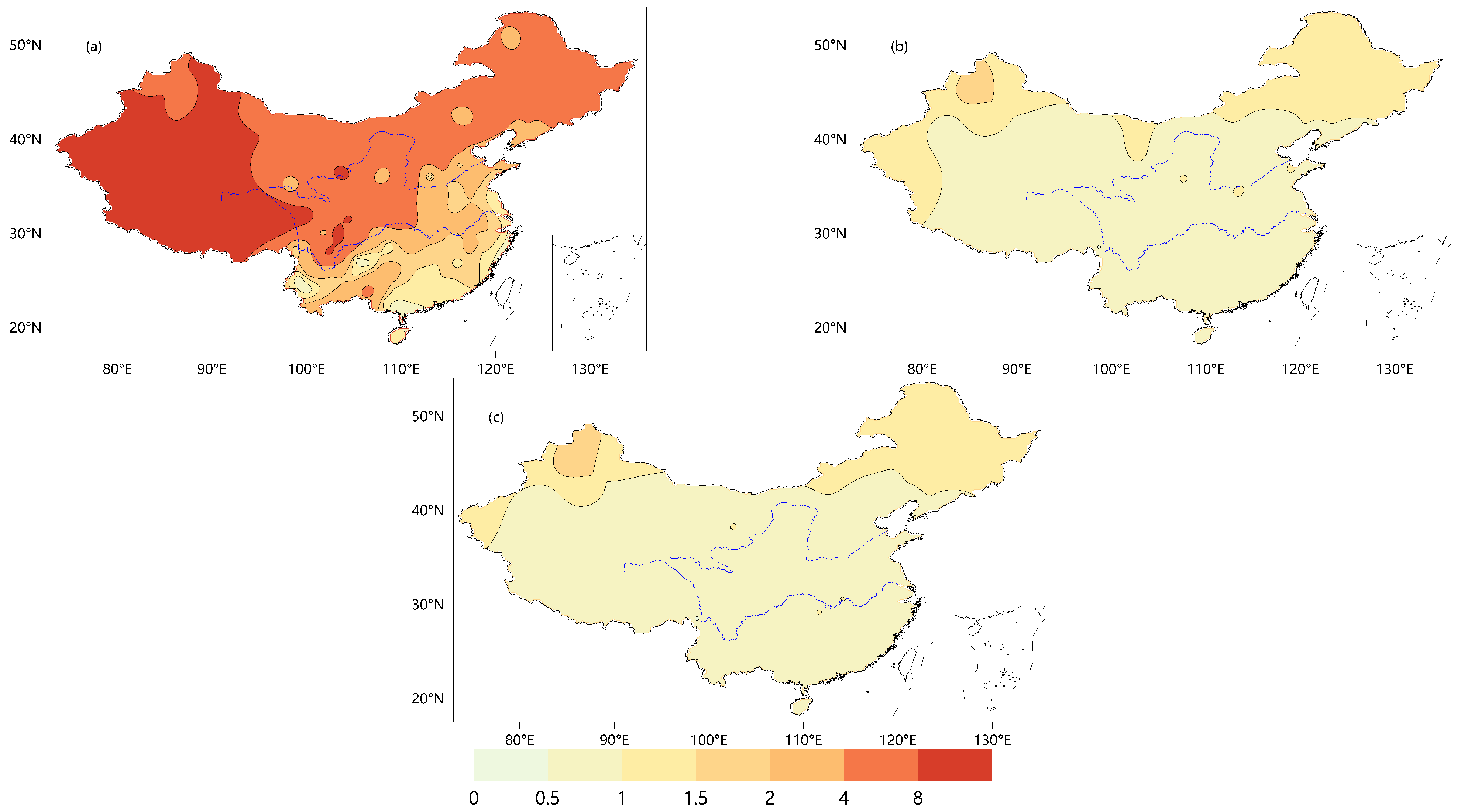
- RMSE
- (b)
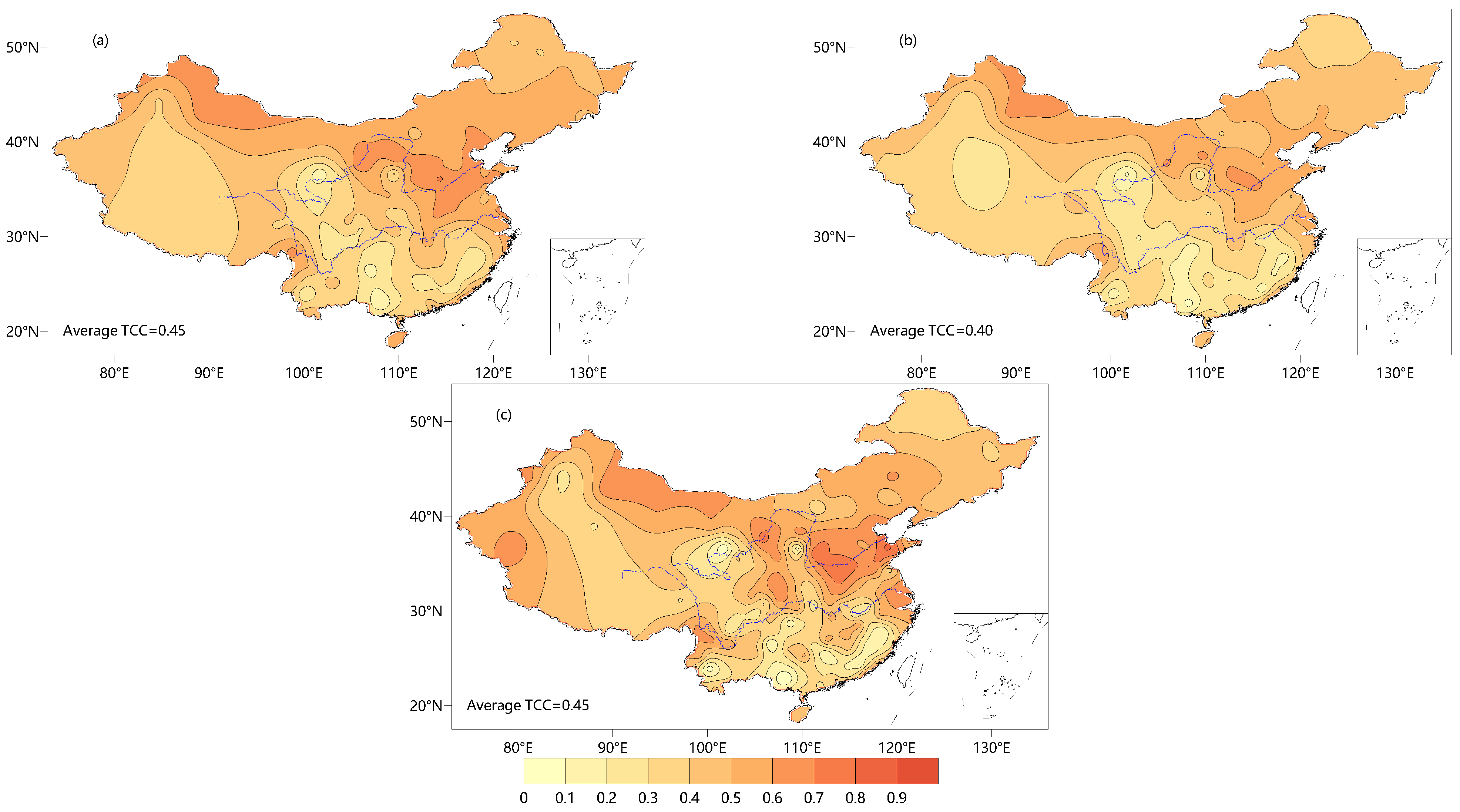
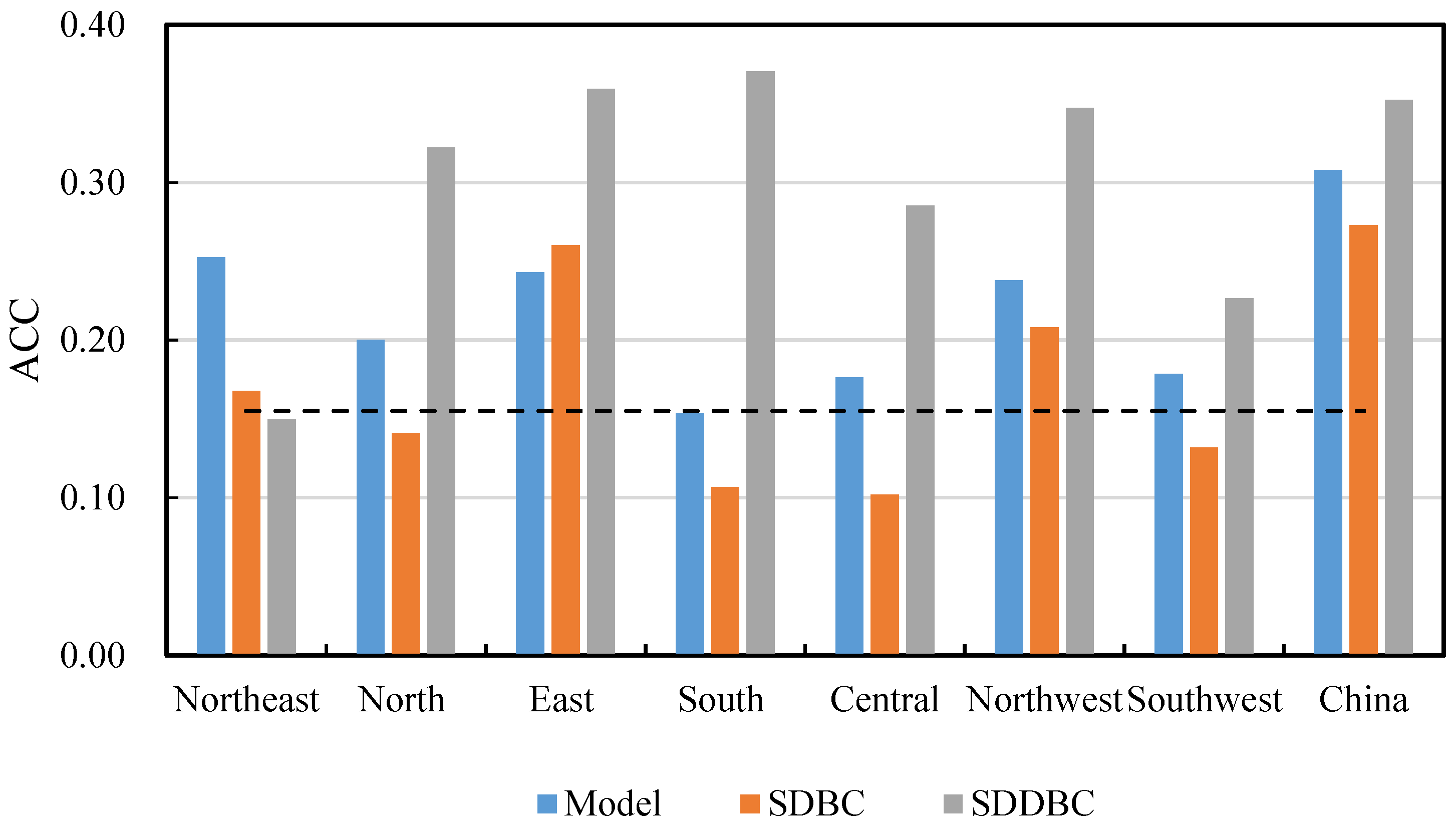
- TCC and ACC
- (c)
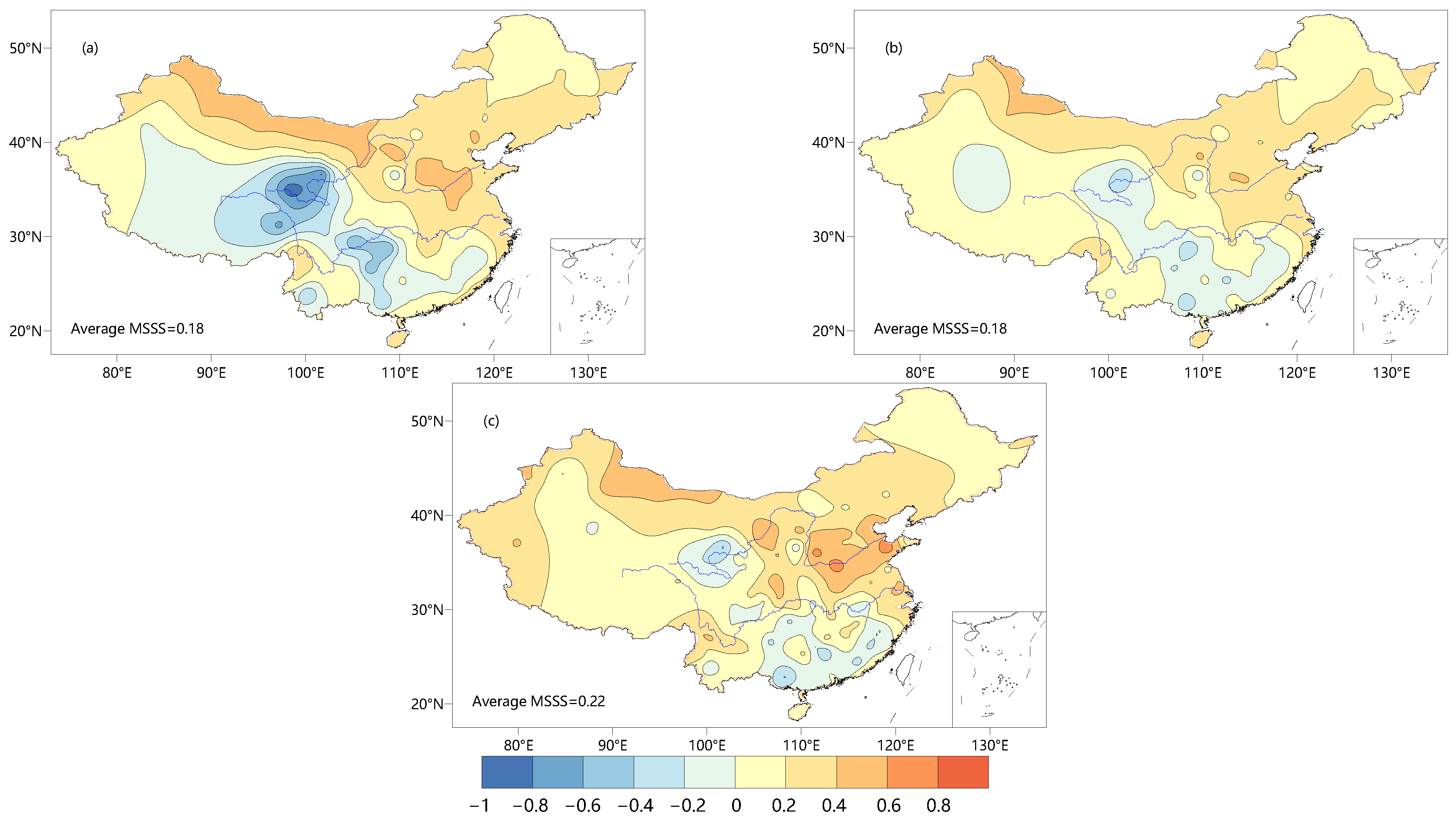
- MSSS
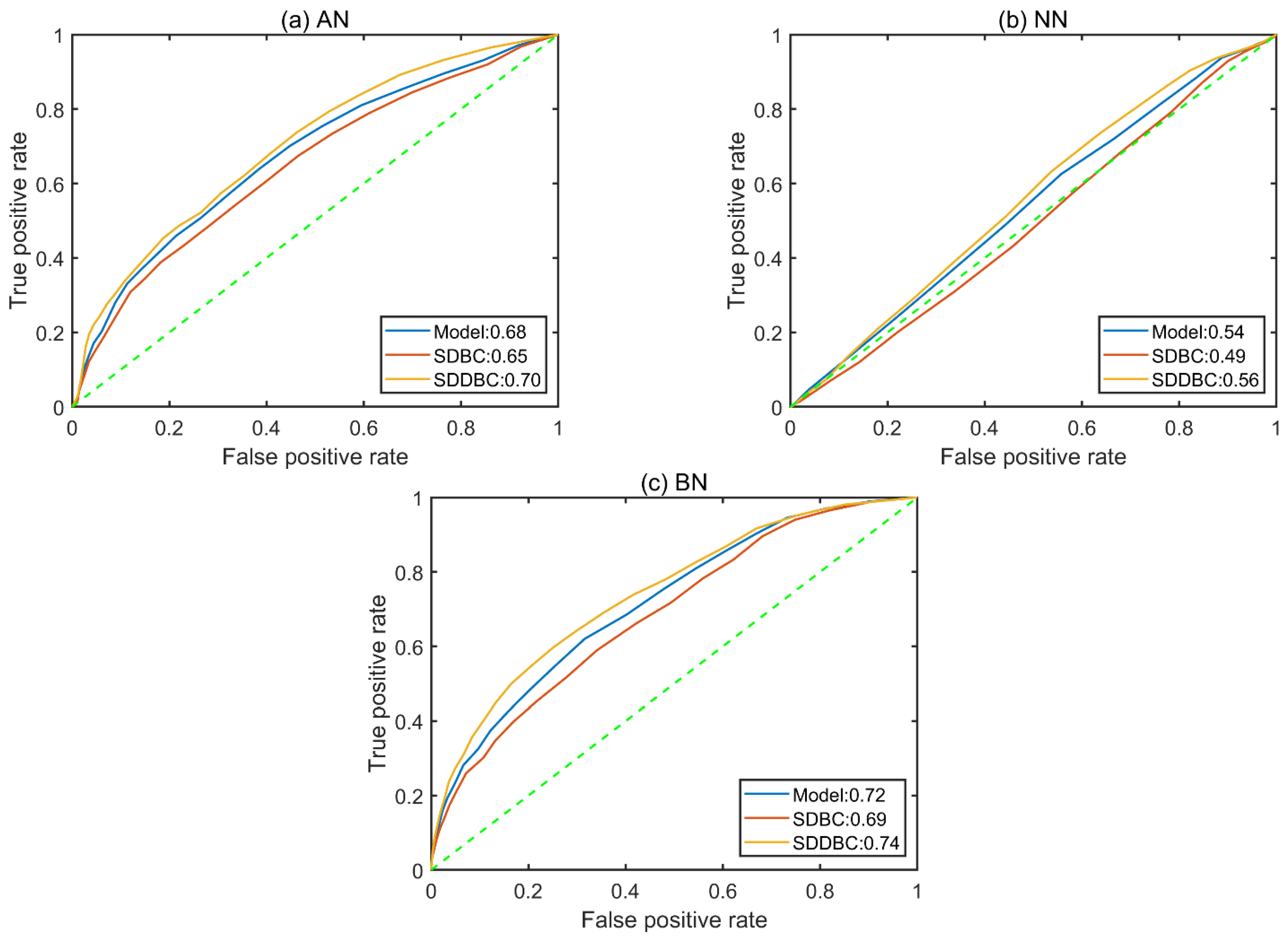
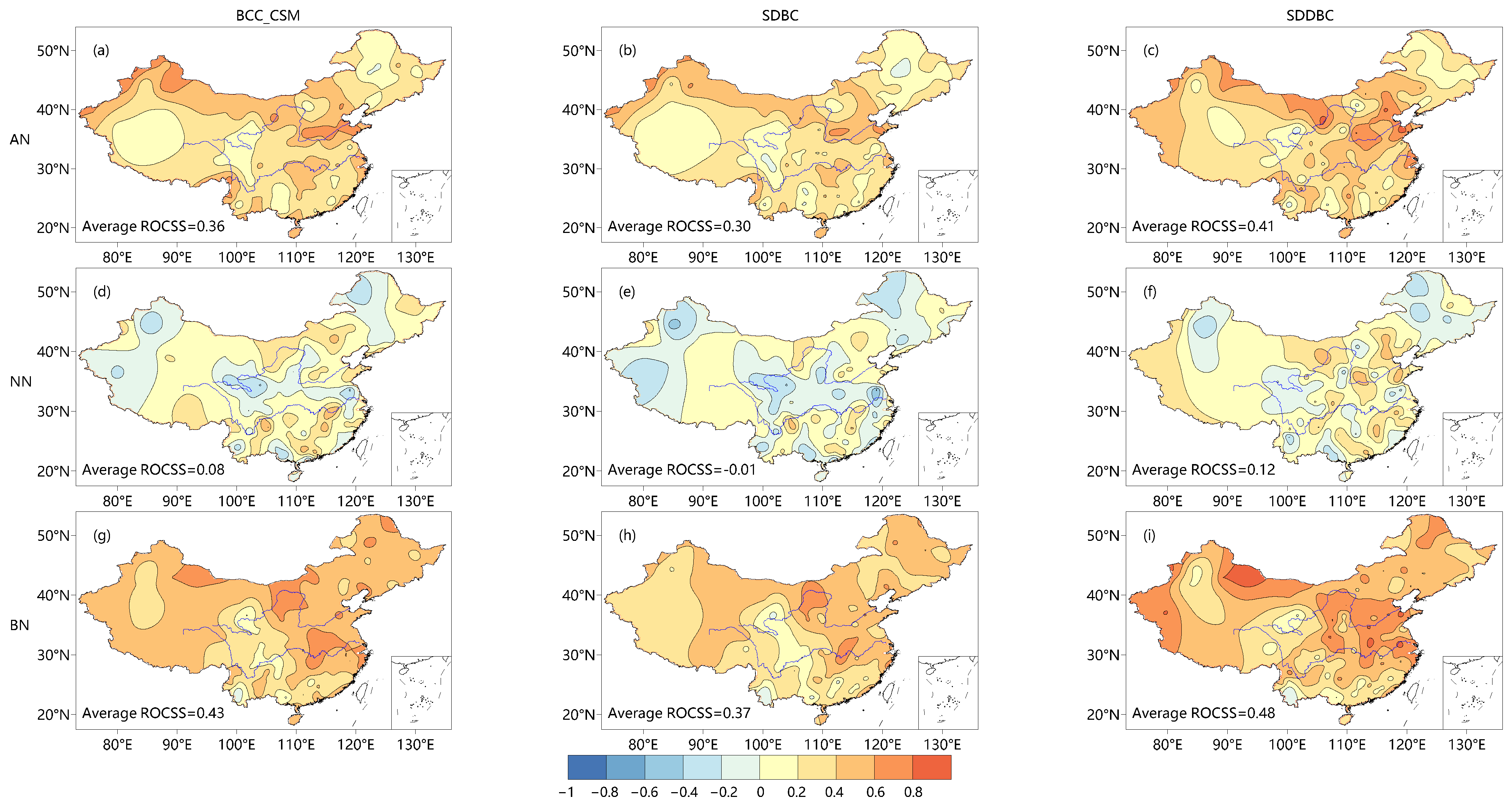
4.3. Probabilistic Evaluation of Forecast Skill
- (a)
- ROC
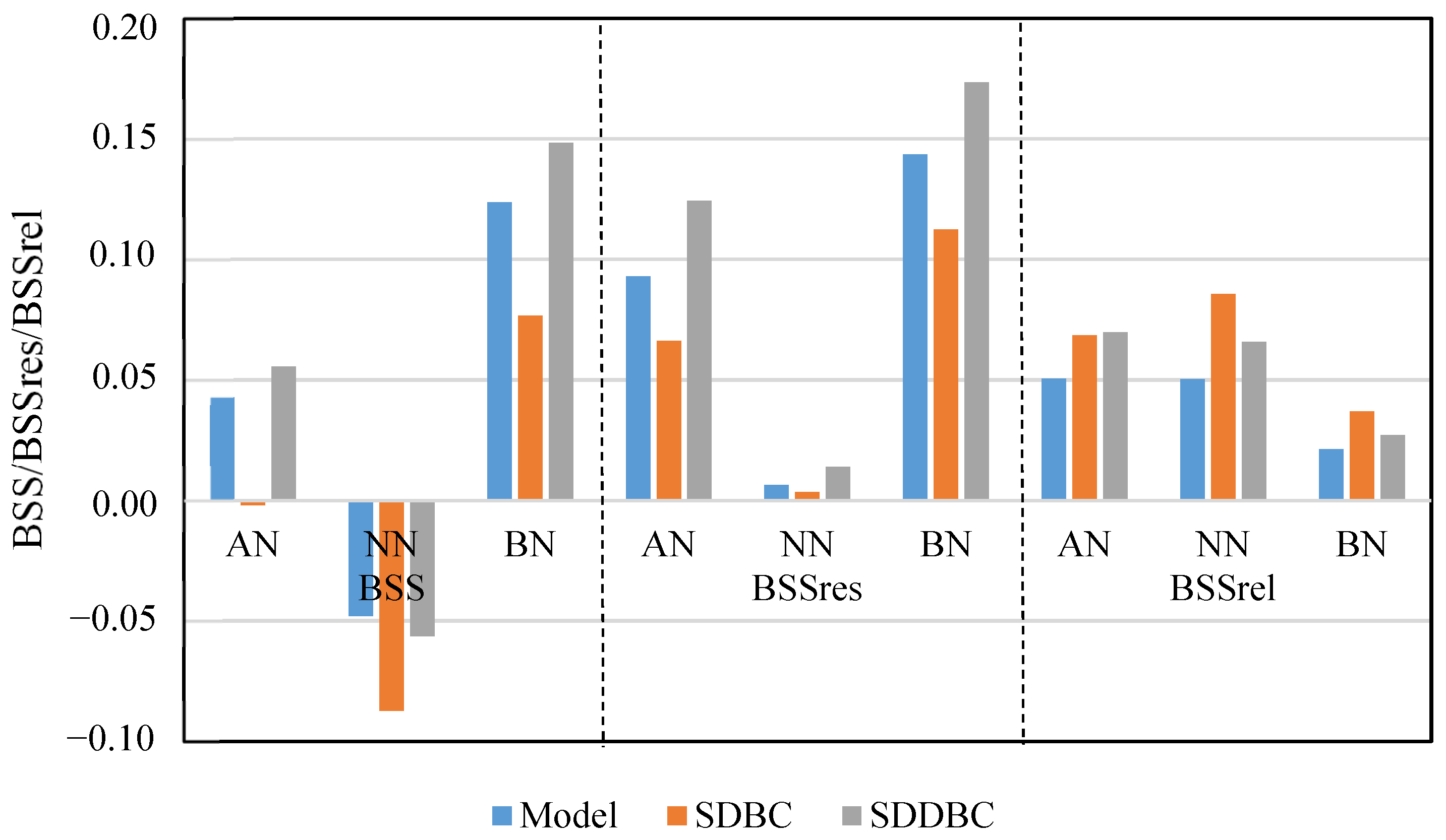
- (b)
- BSS
5. Discussion
6. Conclusions
Author Contributions
Funding
Institutional Review Board Statement
Informed Consent Statement
Data Availability Statement
Acknowledgments
Conflicts of Interest
References
- Saha, S.; Moorthi, S.; Wu, X.; Wang, J.; Nadiga, S.; Tripp, P.; Behringer, D.; Hou, Y.-T.; Chuang, H.-Y.; Iredell, M.; et al. The NCEP climate forecast system version 2. J. Clim. 2014, 27, 2185–2208. [Google Scholar] [CrossRef]
- Johnson, S.J.; Stockdale, T.N.; Ferranti, L.; Balmaseda, M.A.; Molteni, F.; Magnusson, L.; Tietsche, S.; Decremer, D.; Weisheimer, A.; Balsamo, G.; et al. SEAS5, the new ECMWF seasonal forecast system. Geosci. Model. Dev. 2019, 12, 1087–1117. [Google Scholar] [CrossRef] [Green Version]
- Wu, T.; Song, L.; Li, W.; Wang, Z.; Zhang, H.; Xin, X.; Zhang, Y.; Zhang, L.; Li, J.; Wu, F.; et al. An overview of BCC climate system model development and application for climate change studies. J. Meteorol. Res. 2014, 28, 34–56. [Google Scholar] [CrossRef]
- Liu, X.; Wu, T.; Yang, S.; Li, Q.; Cheng, Y.; Liang, X.; Fang, Y.; Jie, W.; Nie, S. Relationships between interannual and intraseasonal variations of the Asian–western Pacific summer monsoon hindcasted by BCC CSM1.1 (m). Adv. Atmos. Sci. 2014, 31, 1051–1064. [Google Scholar] [CrossRef]
- Liu, X.; Wu, T.; Yang, S.; Jie, W.; Nie, S.; Li, Q.; Cheng, Y.; Liang, X. Performance of the seasonal forecasting of the Asian Summer Monsoon by BCC_CSM1.1 (m). Adv. Atmos. Sci. 2015, 32, 1156–1172. [Google Scholar] [CrossRef]
- Ren, H.-L.; Wu, J.; Zhao, C.-B.; Cheng, Y.-J.; Liu, X.-W. MJO ensemble prediction in BCC_CSM1.1 (m) using different initialization schemes. Atmos. Ocean. Sci. Lett. 2016, 9, 60–65. [Google Scholar] [CrossRef]
- Gong, Z.; Dogar, M.M.; Qiao, S.; Hu, P.; Feng, G. Assessment and correction of BCC_CSM’s performance in capturing leading modes of summer precipitation over North Asia. Int. J. Climatol. 2017, 38. [Google Scholar] [CrossRef] [Green Version]
- Zhou, F.; Ren, H.L. Dynamical feedback between synoptic eddy and low-frequency flow as simulated by BCC_CSM1.1 (m). Adv. Atmos. Sci. 2017, 34, 1316–1332. [Google Scholar] [CrossRef]
- Lu, B.; Ren, H.-L.; Eade, R.; Andrews, M. Indian Ocean SST modes and their impacts as simulated in BCC_CSM1.1 (m) and HadGEM3. Adv. Atmos. Sci. 2018, 35, 1035–1048. [Google Scholar] [CrossRef]
- Rao, J.; Ren, R.; Chen, H.; Liu, X.; Yu, Y.; Yang, Y. Sub-seasonal to Seasonal Hindcasts of Stratospheric Sudden Warming by BCC_CSM1.1 (m), A Comparison with ECMWF. Adv. Atmos. Sci. 2019, 36, 17–32. [Google Scholar] [CrossRef]
- Zhou, F.; Ren, H.; Hu, Z.; Liu, M.; Wu, J.; Liu, C. Seasonal Predictability of Primary East-Asian Summer Circulation Patterns by Three Operational Climate Prediction Models. Q. J. R. Meteorol. Soc. 2020, 146, 629–646. [Google Scholar] [CrossRef]
- Liu, Y.; Fan, K.; Chen, L.; Ren, H.-L.; Wu, Y.; Liu, C. An operational statistical downscaling prediction model of the winter monthly temperature over China based on a multi-model ensemble. Atmos. Res. 2021, 249, 105262. [Google Scholar] [CrossRef]
- Wilby, R.; Dawson, C.; Barrow, E. SDSM—A decision support tool for the assessment of regional climate change impacts. Environ. Model. Softw. 2002, 17, 147–159. [Google Scholar] [CrossRef]
- Murphy, J. An evaluation of statistical and dynamical techniques for downscaling local climate. J. Clim. 1999, 12, 2256–2284. [Google Scholar] [CrossRef]
- Xu, C.Y. From GCMs to river flow. A review of downscaling methods and hydrologic modelling approaches. Prog. Phys. Geogr. 1999, 23, 229–249. [Google Scholar] [CrossRef]
- Giorgi, F.; Mearns, L.O. Approaches to the simulation of regional climate change, A review. Rev. Geophys. 1991, 29, 191–216. [Google Scholar] [CrossRef]
- Zhongfeng, X.U.; Han, Y.; Yang, Z. Dynamical downscaling of regional climate, A review of methods and limitations. Sci. China Earth Sci. 2019, 62, 21–31. [Google Scholar] [CrossRef]
- Yoon, J.-H.; Mo, K.; Wood, E. Dynamic-model-based seasonal prediction of meteorological drought over the contiguous United States. J. Hydrometeor. 2012, 13, 463–482. [Google Scholar] [CrossRef]
- Wood, A.; Maurer, E.; Kumar, A.; Lettenmaier, D.P. Long range experimental hydrologic forecasting for the eastern United States. J. Geophys. Res. 2002, 107, 4429. [Google Scholar] [CrossRef]
- Wood, A.; Leung, L.R.; Sridhar, V.; Lettenmaier, D.P. Hydrologic implications of dynamical and statistical approaches to downscaling climate model outputs. Clim. Chang. 2004, 62, 189–216. [Google Scholar] [CrossRef]
- Salathe, E.; Mote, P.W.; Wiley, M.W. Review of scenario selection and downscaling methods for the assessment of climate change impacts on hydrology in the United States Pacific Northwest. Int. J. Climatol. 2007, 27, 1611–1621. [Google Scholar] [CrossRef]
- Maurer, E.P.; Hidalgo, H.G. Utility of daily vs. monthly large-scale climate data, An intercomparison of two statistical downscaling methods. Hydrol. Earth Syst. Sci. 2008, 12, 551–563. [Google Scholar] [CrossRef] [Green Version]
- Tryhorn, L.; Degaetano, A. A comparison of techniques for downscaling extreme precipitation over the Northeastern United States. Int. J. Climatol. 2011, 31, 1975–1989. [Google Scholar] [CrossRef]
- Bürger, G.; Murdock, T.Q.; Werner, A.T.; Sobie, S.R.; Cannon, A. Downscaling Extremes—An Intercomparison of Multiple Statistical Methods for Present Climate. J. Clim. 2012, 25, 4366–4388. [Google Scholar] [CrossRef]
- Sharma, D.; Babel, M.S. Application of downscaled precipitation for hydrological climate-change impact assessment in the upper Ping River Basin of Thailand. Clim. Dyn. 2013, 41, 2589–2602. [Google Scholar] [CrossRef]
- Lin, W.; Wen, C. A CMIP5 multimodel projection of future temperature, precipitation, and climatological drought in China. Int. J. Climatol. 2014, 34, 2059–2078. [Google Scholar] [CrossRef]
- Sharma, D.; Babel, M.S. Assessing hydrological impacts of climate change using bias-corrected downscaled precipitation in Mae Klong basin of Thailand. Meteorol. Appl. 2017, 25, 384–393. [Google Scholar] [CrossRef]
- Shrestha, R.R.; Schnorbus, M.A.; Cannon, A.J. A Dynamical Climate Model-Driven Hydrologic Prediction System for the Fraser River, Canada. J. Hydrometeorol. 2015, 16, 150206095227003. [Google Scholar] [CrossRef]
- Touseef, M.; Chen, L.; Yang, K.; Chen, Y. Long-Term Rainfall Trends and Future Projections over Xijiang River Basin, China. Adv. Meteorol. 2020, 2020, 6852148. [Google Scholar] [CrossRef] [Green Version]
- Lorenz, C.; Portele, T.C.; Laux, P.; Kunstmann, H. Bias-corrected and spatially disaggregated seasonal forecasts, a long-term reference forecast product for the water sector in semi-arid regions. Earth Syst. Sci. Data 2021, 13, 2701–2722. [Google Scholar] [CrossRef]
- Abatzoglou, J.T.; Brown, T.J. A comparison of statistical downscaling methods suited for wildfire applications. Int. J. Climatol. 2012, 32, 772–780. [Google Scholar] [CrossRef]
- Hwang, S.; Graham, W.D. Development and comparative evaluation of a stochastic analog method to downscale daily GCM precipitation. Hydrol. Earth Syst. Sci. Discuss. 2013, 10, 2141–2181. [Google Scholar] [CrossRef] [Green Version]
- Tian, D.; Martinez, C.J.; Graham, W.D. Seasonal Prediction of Regional Reference Evapotranspiration Based on Climate Forecast System Version 2. J. Hydrometeorol. 2014, 15, 1166–1188. [Google Scholar] [CrossRef]
- Tian, D.; Martinez, C.J.; Graham, W.D.; Hwang, S. Statistical Downscaling Multimodel Forecasts for Seasonal Precipitation and Surface Temperature over the Southeastern United States. J. Clim. 2014, 27, 8384–8411. [Google Scholar] [CrossRef]
- Ali, S.; Eum, H.-I.; Cho, J.; Dan, L.; Khan, F.; Dairaku, K.; Shrestha, M.L.; Hwang, S.; Nasim, W.; Khan, I.A.; et al. Assessment of climate extremes in future projections downscaled by multiple statistical downscaling methods over Pakistan. Atmos. Res. 2019, 222, 114–133. [Google Scholar] [CrossRef]
- Schaake, J.; Demargne, J.; Hartman, R.; Mullusky, M.; Welles, E.; Wu, L.; Herr, H.; Fan, X.; Seo, D.J. Precipitation and temperature ensemble forecasts from single-value forecasts. Hydrol. Earth Syst. Sci. Discuss. 2007, 4, 655–717. [Google Scholar] [CrossRef] [Green Version]
- Wood, A.W.; Schaake, J.C. Correcting errors in streamflow forecast ensemble mean and spread. J. Hydrometeor. 2008, 9, 132–148. [Google Scholar] [CrossRef]
- Luo, L.; Wood, E.F. Use of Bayesian merging techniques in a multimodel seasonal hydrologic ensemble prediction system for the eastern United States. J. Hydrometeor. 2008, 9, 866–884. [Google Scholar] [CrossRef]
- Luo, L.; Wood, E.F.; Pan, M. Bayesian merging of multiple climate model forecasts for seasonal hydrological predictions. J. Geophys. Res. 2007, 112, D10102. [Google Scholar] [CrossRef] [Green Version]
- Pierce, D.W.; Cayan, D.R.; Thrasher, B.L. Statistical Downscaling Using Localized Constructed Analogs (LOCA). J. Hydrometeorol. 2014, 15, 2558–2585. [Google Scholar] [CrossRef]
- Chang, S.; Graham, W.; Geurink, J.; Wanakule, N.; Asefa, T. Evaluation of impacts of future climate change and water use scenarios on regional hydrology. Hydrol. Earth Syst. Sci. 2018, 22, 4793–4813. [Google Scholar] [CrossRef] [Green Version]
- Chang, S.; Graham, W.; Geurink, J.; Asefa, T. Evaluation of impact of climate change and anthropogenic change on regional hydrology. Hydrol. Earth Syst. Sci. Discuss. 2018, 3, 1–43. [Google Scholar] [CrossRef]
- Maurer, E.; Hidalgo, H.; Das, T.; Dettinger, M.D.; Cayan, D.R. The utility of daily large-scale climate data in the assessment of climate change impacts on daily streamflow in California. Hydrol. Earth Syst. Sci. 2010, 14, 1125–1138. [Google Scholar] [CrossRef] [Green Version]
- Tian, D.; Martinez, C.J. Forecasting reference evapotranspiration using retrospective forecast analogs in the southeastern United States. J. Hydrometeor. 2012, 13, 1874–1892. [Google Scholar] [CrossRef]
- Tian, D.; Martinez, C.J. Comparison of two analog-based downscaling methods for regional reference evapotranspiration forecasts. J. Hydrol. 2012, 475, 350–364. [Google Scholar] [CrossRef]
- Wang, S.; Zhu, J. A review on seasonal climate prediction. Adv. Atmos. Sci. 2001, 18, 197–208. [Google Scholar] [CrossRef]
- Li, Q.; Sun, W.; Yun, X.; Huang, B.; Dong, W.; Wang, X.L.; Zhai, P.; Jones, P. An updated evaluation of the global mean Land Surface Air Temperature and Surface Temperature trends based on CLSAT and CMST. Clim. Dyn. 2021, 56, 635–650. [Google Scholar] [CrossRef]
- Xin, X.-G.; Wu, T.-W.; Li, J.-L.; Wang, Z.Z.; Li, W.; Wu, F.-H. How Well does BCC_CSM1.1 Reproduce the 20th Century Climate Change over China? Atmos. Ocean. Sci. Lett. 2013, 6, 21–26. [Google Scholar] [CrossRef] [Green Version]
- Papalexiou, S.M.; Rajulapati, C.R.; Clark, M.P.; Lehner, F. Robustness of CMIP6 Historical Global Mean Temperature Simulations, Trends, Long-Term Persistence, Autocorrelation, and Distributional Shape. Earth Future 2020, 8. [Google Scholar] [CrossRef]
- Kumar, S.; Kinter, J.L.; Pan, Z.; Sheffield, J. Twentieth century temperature trends in CMIP3, CMIP5, and CESM-LE climate simulations spatial-temporal uncertainties, differences and their potential sources. J. Geophys. Res. Atmos. 2016, 121, 9561–9575. [Google Scholar] [CrossRef]
- Wen, C.; Duan, C.; Shen, S.; Yao, Y. Evaluation and Parameter Optimization of Monthly Net Long-Wave Radiation Climatology Methods in China. Atmosphere 2017, 8, 94. [Google Scholar] [CrossRef] [Green Version]
- Stanski, H.R.; Wilson, L.J.; Burrows, W.R. Survey of Common Verification Methods in Meteorology; World Weather Watch Technical Report No. 8, WMO/TD No. 358; World Meteorological Organization: Geneva, Switzerland, 1998; p. 17. [Google Scholar]
- Wilks, D.S. Statistical Methods in the Atmospheric Sciences; Academic Press: Cambridge, MA, USA; Elsevier: Amsterdam, The Netherlands, 2011; pp. 328–340. [Google Scholar]
- World Meteorological Organization. Standardised Verification System (SVS) for Long-Range Forecasts (LRF); New Attachment II-8 to the Manual on the GDPFS (WMO-No. 485); World Meteorological Organization: Geneva, Switzerland, 2006; Volume I, pp. 68–80. [Google Scholar]
- Murphy, A.H. Skill scores based on the mean square error and their relationships to the correlation coefficient. Mon. Weather Rev. 1988, 16, 2417–2424. [Google Scholar] [CrossRef]
- Hamill, T.M.; Juras, J. Measuring forecast skill, is it real skill or is it the varying climatology? Q. J. R. Meteorol. Soc. 2006, 132, 2905–2923. [Google Scholar] [CrossRef] [Green Version]


| Region | MSSS | Phase Skills | Amplitude Errors | ||||||
|---|---|---|---|---|---|---|---|---|---|
| Model | SDBC | SDDBC | Model | SDBC | SDDBC | Model | SDBC | SDDBC | |
| Northeast China | 0.23 | 0.20 | 0.18 | 0.77 | 0.61 | 0.61 | 0.59 | 0.47 | 0.49 |
| North China | 0.29 | 0.25 | 0.31 | 0.74 | 0.58 | 0.74 | 0.49 | 0.38 | 0.49 |
| East China | 0.23 | 0.20 | 0.26 | 0.51 | 0.48 | 0.69 | 0.33 | 0.37 | 0.53 |
| South China | 0.05 | −0.01 | −0.03 | 0.43 | 0.40 | 0.42 | 0.44 | 0.48 | 0.52 |
| Central China | 0.21 | 0.18 | 0.24 | 0.51 | 0.45 | 0.64 | 0.38 | 0.37 | 0.52 |
| Northwest China | 0.22 | 0.22 | 0.27 | 0.58 | 0.50 | 0.68 | 0.51 | 0.41 | 0.53 |
| Southwest China | −0.13 | 0.04 | 0.11 | 0.55 | 0.33 | 0.51 | 0.74 | 0.35 | 0.48 |
| China | 0.18 | 0.18 | 0.22 | 0.58 | 0.48 | 0.63 | 0.50 | 0.40 | 0.51 |
| Region | Above Normal | Near Normal | Below Normal | ||||||
|---|---|---|---|---|---|---|---|---|---|
| Model | SDBC | SDDBC | Model | SDBC | SDDBC | Model | SDBC | SDDBC | |
| Northeast China | −0.07 | −0.13 | −0.11 | −0.02 | −0.07 | −0.09 | 0.16 | 0.12 | 0.14 |
| North China | 0.07 | 0.03 | 0.11 | −0.04 | −0.07 | −0.03 | 0.18 | 0.14 | 0.22 |
| East China | 0.06 | 0.01 | 0.08 | −0.04 | −0.08 | −0.05 | 0.18 | 0.13 | 0.21 |
| South China | −0.02 | −0.07 | 0.00 | −0.08 | −0.12 | −0.07 | 0.02 | −0.04 | −0.02 |
| Central China | 0.07 | 0.03 | 0.08 | −0.03 | −0.08 | −0.05 | 0.20 | 0.15 | 0.23 |
| Northwest China | 0.09 | 0.05 | 0.12 | −0.09 | −0.12 | −0.05 | 0.11 | 0.07 | 0.17 |
| Southwest China | 0.04 | −0.01 | 0.03 | −0.03 | −0.07 | −0.07 | 0.02 | −0.03 | 0.05 |
| China | 0.04 | 0.00 | 0.06 | −0.05 | −0.09 | −0.06 | 0.12 | 0.08 | 0.15 |
Publisher’s Note: MDPI stays neutral with regard to jurisdictional claims in published maps and institutional affiliations. |
© 2021 by the authors. Licensee MDPI, Basel, Switzerland. This article is an open access article distributed under the terms and conditions of the Creative Commons Attribution (CC BY) license (https://creativecommons.org/licenses/by/4.0/).
Share and Cite
Duan, C.; Wang, P.; Cao, W.; Wang, X.; Wu, R.; Cheng, Z. Improving the Spring Air Temperature Forecast Skills of BCC_CSM1.1 (m) by Spatial Disaggregation and Bias Correction: Importance of Trend Correction. Atmosphere 2021, 12, 1143. https://doi.org/10.3390/atmos12091143
Duan C, Wang P, Cao W, Wang X, Wu R, Cheng Z. Improving the Spring Air Temperature Forecast Skills of BCC_CSM1.1 (m) by Spatial Disaggregation and Bias Correction: Importance of Trend Correction. Atmosphere. 2021; 12(9):1143. https://doi.org/10.3390/atmos12091143
Chicago/Turabian StyleDuan, Chunfeng, Pengling Wang, Wen Cao, Xujia Wang, Rong Wu, and Zhi Cheng. 2021. "Improving the Spring Air Temperature Forecast Skills of BCC_CSM1.1 (m) by Spatial Disaggregation and Bias Correction: Importance of Trend Correction" Atmosphere 12, no. 9: 1143. https://doi.org/10.3390/atmos12091143
APA StyleDuan, C., Wang, P., Cao, W., Wang, X., Wu, R., & Cheng, Z. (2021). Improving the Spring Air Temperature Forecast Skills of BCC_CSM1.1 (m) by Spatial Disaggregation and Bias Correction: Importance of Trend Correction. Atmosphere, 12(9), 1143. https://doi.org/10.3390/atmos12091143