Mapping Nighttime and All-Day Radiative Cooling Potential in Europe and the Influence of Solar Reflectivity

Abstract

Radiative cooling is a natural process to cool down surfaces through the rejection of thermal radiation using the outer space as a cold sink, taking advantage of the transparency of the atmospheric windows (8–14 μm), which partially matches the infrared radiation band. With the development of new materials that have a high reflectivity of solar radiation, daytime radiative cooling can be achieved. This phenomenon depends on the optical properties of the surface and the local weather conditions. In this research, climatological data from 1791 weather stations were used to present detailed nighttime and all-day radiative cooling maps for the potential implementation of radiative cooling-based technologies. The paper offers a parametric study of the variation of the potential as a result of decreasing the solar reflectivity. The results show that southern Europe is the region with the highest potential while northern Europe holds more hours of available radiative cooling. After varying the solar reflectivity from 1 to 0.5 the average power reduces from 60.18 to 45.32 W/m², and energy from 527.10 to 264.87 kWh/m²·year. For solar reflectivity lower than 0.5, all-day radiative coolers behave as nighttime radiative coolers, but power and energy values improve significantly for high values of solar reflectivity. Small variations of solar reflectivity have greater impacts on the potential at higher reflectivity values than at lower ones.

1. Introduction

Radiative cooling (RC) is a natural cooling process already used in 400 BC in ancient Iran for ice production [1]. In recent years it has experienced a new awakening. During the 1960s and 1970s the phenomenon began to be studied systematically [2,3]. However, it is in this last decade, driven by the needs for a change in the model of energy production and consumption, when technologies based on RC are positioned as promising solutions for the production of clean and green energies for space cooling purposes.

Radiative cooling is known to be the process by which a surface reduces its temperature through the emission of thermal radiation into the outer space. It benefits from the high transparency of the atmosphere in 8–14 μm wavelength range, named atmospheric window, which partially matches the peak of infrared radiation emitted by terrestrial bodies at ambient temperatures. This cooling process occurs when a net imbalance exists between the emitted and the absorbed heat; solar radiation, atmospheric radiation and parasitic losses (convection and conduction) also accounted for in this net balance. This technique allows for achieving temperatures below ambient [4].

The first selective surfaces (also called emitters), emitting in the 8–14 μm range, were designed to achieve RC during night time [2,5]. In 1975, Catalanotti et al. [3] obtained radiative cooling during daytime, but the performance was poor. Overcoming solar radiation was a great challenge. In 2014, Raman et al. [6] demonstrated a temperature drop—4–5 °C—below ambient under direct sunlight in photonic radiative cooling, which combined layers of SiO₂ and HfO₂ on top of a silver surface. The recent development of new multilayer thin structures [6,7,8], porous polymers [9,10,11], nanoparticle materials [12], metamaterials [13,14,15,16] and photonic crystals [17,18,19], allows the manufacture of selective surfaces which emit only in the 8–14 μm range while reflecting the incoming solar radiation.

Several authors have conducted simulation studies in order to predict the potential of radiative cooling technologies. Vall et al. [20] modelled the behavior of a system that combined solar collection and radiative cooling in order to determine the potential coverage of cooling and DHW requirements in residential and commercial buildings under different climates. Feng et al. [21] conducted a daytime RC simulation and experimentation and evaluated the most significate variables and concluded that, in order to maximize RC, ultra-low parasitic heat gains and maximum suppression of solar irradiance in the emitter was required. Bijarniya et al. [22] studied the radiative cooling potential in various climate conditions in five cities in India, and evaluated the performance of different RC systems (ideal emitters, broadband emitters and selective emitters). Carlosena et al. [23] studied the potential of daytime radiative cooling for mitigating the effects of urban heat islands and performed simulations of different applications and locations for a total of 15 theoretical materials and 7 existing materials used in emitters.

Prediction of radiative cooling potential in different areas could become an aid to drive public policies on the usage of renewable energies. In 1992, Argiriou et al. [24] estimated the sky temperature depression and the night time performance of a RC flat plate in different countries in southern Europe, and concluded that southern Europe exhibited a promising potential for a high application of this technology. Chang et al. [25] and Li et al. [26] used geostatistical prediction tools to model and to obtain radiative cooling potential maps in China and USA, respectively.

In this research we applied interpolation tools to generate annual nighttime and all-day radiative cooling potential maps in Europe. A comparison of results between emitters with different reflectivity in the solar range is also offered. We present twenty maps corresponding to seven maps of annual power, seven maps of annual energy production and six maps of percentage of RC hours over total annual hours.

2. Methods

The parametric study of the variation of the all-day radiative cooling potential in Europe as a function of the reflectivity in the solar range of the emitter material was conducted based on meteorological data measured in 1791 weather stations. Kriging was the interpolation technique used to obtain radiative cooling maps.

2.1. Data Acquisition

The climatological data used was available in the Meteornorm database. Meteonorm is a recognized software in the field of energy simulation of buildings and solar facilities. The downloaded data corresponded to a total of 1791 weather stations distributed in 46 European countries. The distribution of these stations is shown in Figure 1. The data is related to the last volume of measured data available in Metonorm for the year 2005. The resulting dataset included information on weather variables recorded hourly for 365 days of the year. Stored variables included ambient temperature, atmospheric IR radiation and global horizontal solar radiation, relative humidity, clearness index of the sky and atmospheric pressure. Ambient temperature, global horizontal solar radiation, relative humidity, clearness index or atmospheric pressure are data measured at the weather station while atmospheric radiation (L_in) is calculated based on the Aubinet model (1) [27]:

$$L_{in}=\sigma ·{\left[94+12.6\log \left(100·e_s\right)-13·K{T}_d+0.341·\left(T_a+273.15\right)\right]}^4$$

(1)

where $L_{in}$ is the atmospheric radiation (W/m²); σ is the Stefan–Boltzman constant $\left(\mathrm{W}\frac{{\mathrm{m}}^2}{{\mathrm{K}}^4}\right)$; e_s is the saturated vapor pressure (hPa); KT_d is the clearness index (-) and T_a is the ambient temperature (°C).

2.2. Radiative Cooling Calculation

In the research, the following premises were assumed: the greatest potential of a black-body surface (emittance of the surface (ε_s) equal to one) (a) could be achieved by minimizing the parasitic losses of conduction and convection, (b) while absorbed solar radiation depended on the reflectivity of the surface. In this study, ε_s is equal to 1 and parasitic losses are neglected. In RC applications, the emitter surface temperature is close to ambient temperature; in this case it was assumed that (c) the temperature on the surface was equal to ambient temperature. The net balance power per surface unit at each location was calculated (2).

$$q_{\mathit{net},\mathit{ideal}}\left(T_a\right)=\sigma T_a^4-L_{in}-\left(1-\rho \right)S_H\hspace{1em}\left(\mathrm{W}/{\mathrm{m}}^2\right)$$

(2)

where $\rho$ is the solar reflectivity of the emitter (-) and $S_H$ corresponds to the global horizontal solar radiation (W/m²).

Only positive values of Equation (2), corresponding to observations where radiative cooling occurred, were filtered. The average annual RC potential at each location was calculated according to (3) where $n$ is the total number of positive observations:

$$q_{\mathit{rc},\mathit{avg}}=\frac{{{\displaystyle \sum }}_i^n{q}_{\mathit{net},\mathit{ideal}}{}^{+}}{n}\hspace{1em}\left(\mathrm{W}/{\mathrm{m}}^2\right)$$

(3)

Every value from Equation (2) corresponded to a one-hour observation (t = 1 h). Thus, allowing us to calculate the RC annual energy (6):

$$e_{\mathit{rc}}=\frac{{{\displaystyle \sum }}_i^n{q}_{\mathit{net},\mathit{ideal}}{}^{+}·t}{1000}\left(\frac{\mathrm{kWh}}{{\mathrm{m}}^2}·\mathrm{year}\right)$$

(4)

Finally, a third value was included (5). This value referred to the number of observations where radiative cooling was achieved ($N\left[q_{\mathit{net},\mathit{ideal}}{}^{+}\right]$), compared to the total number of observations ($8760$).

$$\mathit{coverage}=\frac{N\left(q_{\mathit{net},\mathit{ideal}}{}^{+}\right)}{8760}\hspace{1em}[\%]$$

(5)

2.3. Training and Test Datasets

Data was divided into two subsets: training set and test set. The training set contained information from 80% of the locations and was used in the construction of the interpolation model for each value of $\rho$. Test set data was used to evaluate the performance of each model.

2.4. Interpolation Kriging Model

Kriging is a stochastic interpolation method for values prediction at different points from known reference values. In the study we used the most general version of the methodology, ordinary Kriging, which decomposed the regressor into a stationary part $\left(\mu \right)$ and a residual $\left({\epsilon }^{\prime }\right)$, corresponding to the spatially correlated part (6) [28]:

$$Z\left(s\right)=\mu +{\epsilon }^{\prime }\left(s\right)$$

(6)

This method worked as a linear regression applied to spatial sample data which was used as regressor, $Z\left(s\right)$, in order to predict a dependent variable, $Z\left(s_0\right),$ at a given location (7). The weight given by the model to each of the points in the sample was determined by a variogram function (8).

$$\widehat{Z}\left(s_0\right)={\lambda }_{0}Z\left(s\right)$$

(7)

$$\left(\begin{array}{cc}\begin{array}{ccc}\gamma \left(s_1-s_1\right)& \dots & \gamma \left(s_1-s_n\right)\\ ⋮& \ddots & ⋮\\ \gamma \left(s_n-s_1\right)& \dots & \gamma \left(s_n-s_n\right)\end{array}& \begin{array}{c}1\\ 1\\ 1\end{array}\\ \begin{array}{ccc}1& \dots & 1\end{array}& 0\end{array}\right)·{\lambda }_0=\left(\begin{array}{c}\gamma \left(s_1-s_0\right)\\ ⋮\\ \begin{array}{c}\gamma \left(s_n-s_0\right)\\ 1\end{array}\end{array}\right)$$

(8)

where λ₀ is a vector of Kriging weights, n the number of sample points and $\gamma$ is the semivariance.

The semivariance of the sample was calculated for each pair of points from (9), where $Z\left(s_i\right)$ is the value of the target variable at the point $s_i$, $Z\left(s_i+h\right)$ is the value of the neighbor point at a distance $s_i+h$ and E corresponds to the expected value. A theoretical variogram was adjusted to the variogram so that the error of the fitting was minimum.

$$\gamma \left(h\right)=\frac{1}{2} E\left[{\left(Z\left(s_i\right)-Z\left(s_i+h\right)\right)}^2\right]$$

(9)

2.5. Assessment Metrics of the Model

Radiative cooling values were predicted using the test set locations in the Kriging model. These predictions were compared with the existing potential values at these locations. In order to evaluate the accuracy of the model, the coefficient of determination (R²) and the root mean square error (RMSE) were calculated (10) and (11):

$$R^2=1-\frac{{{\displaystyle \sum }}_{i=1}^N{\left(X_{i,m}-X_{i,p}\right)}^2}{{{\displaystyle \sum }}_{i=1}^N{\left(X_{i,m}-X_{m,\mathit{avg}}\right)}^2}$$

(10)

$$\mathit{RMSE}=\sqrt{\frac{1}{N}{{\displaystyle \sum }}_{i=1}^N{\left(X_{i,m}-X_{i,p}\right)}^2}$$

(11)

where $N$ is the total number of locations; $X_{i,m}$ is the observed values of the sample; $X_{i,p}$ is the value estimated in the model and $X_{m,\mathit{avg}}$ is the average of the observed values at the weather stations. RMSE has the same units as the variable at interpolation (power, energy and coverage) while R² is dimensionless.

3. Results and Discussion

In the first part of this section we present a comparison of the prediction maps for the cases of nighttime and all-day RC of an ideal reflective surface ($\rho$ = 1). In the second part we determine the changes that occur when varying the value of surface reflectivity in all-day RC. In both sections the performance of the interpolation models used has been evaluated.

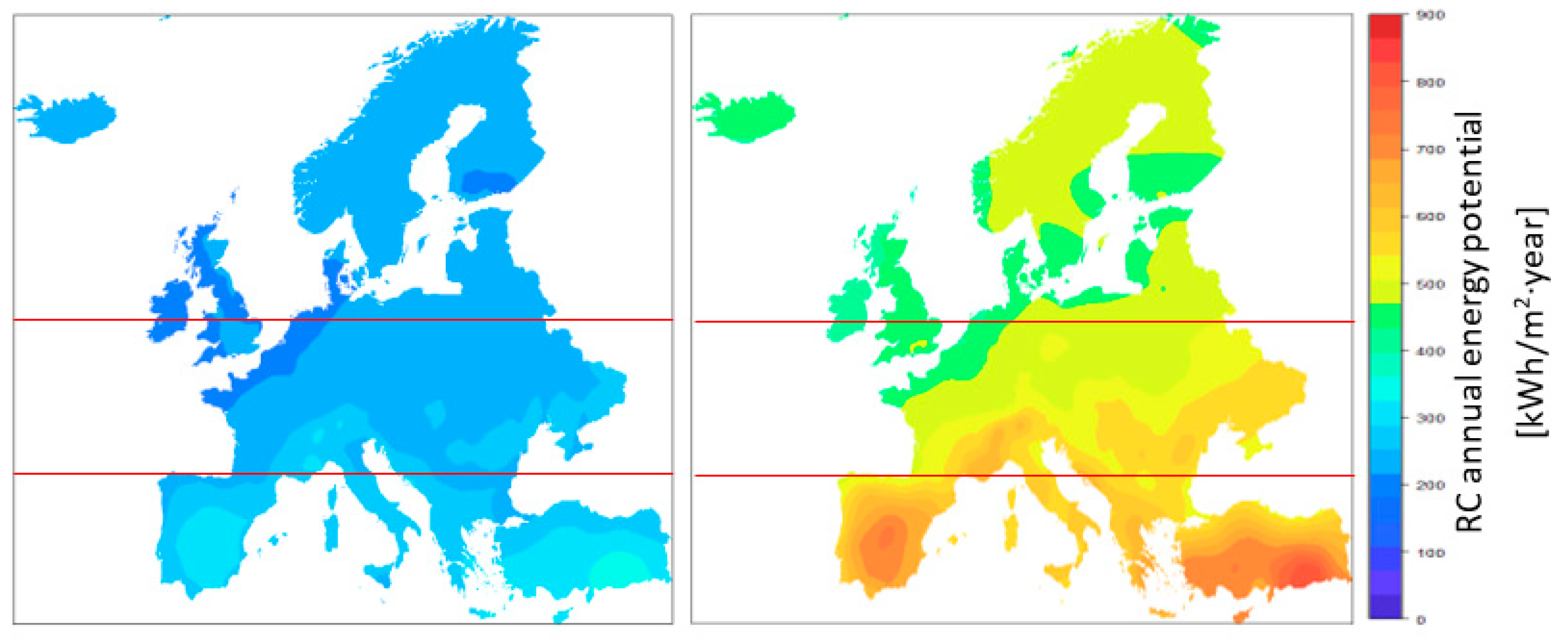
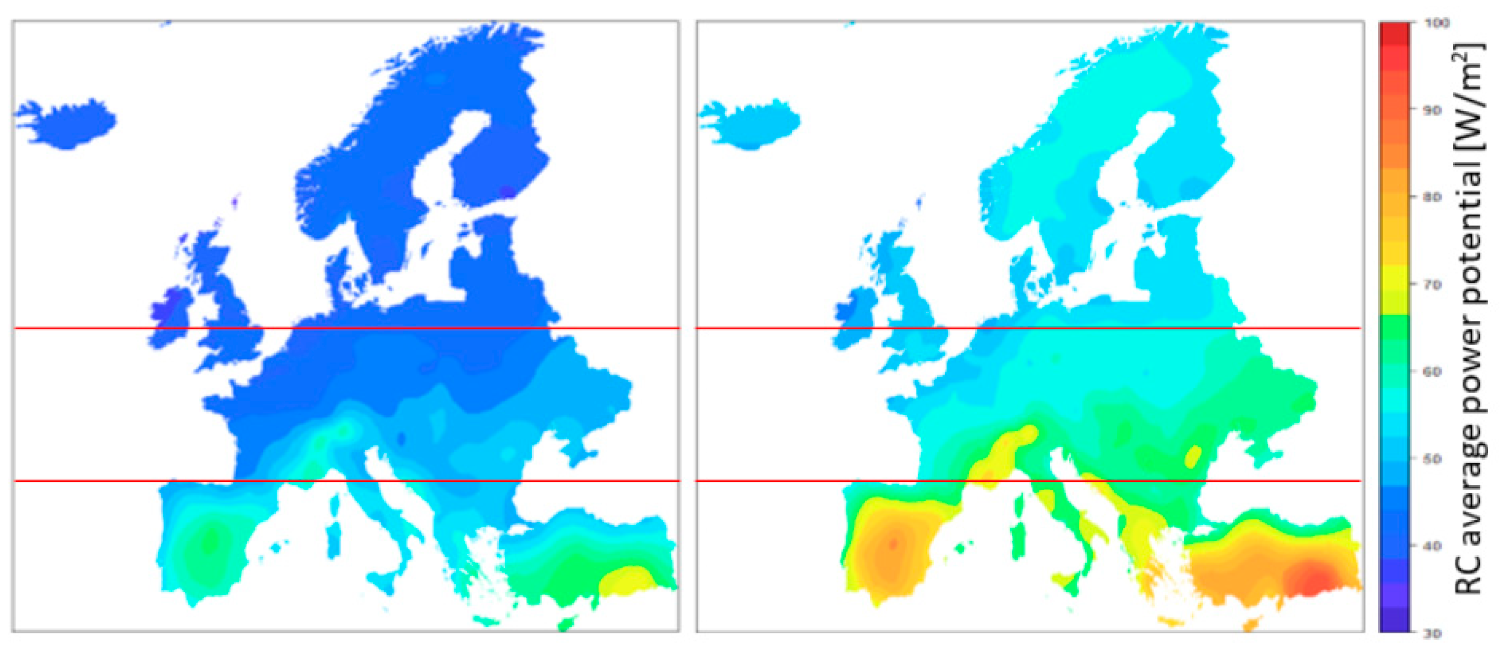
3.1. Nighttime and All-Day Comparison

Figure 2 shows the annual potential maps of radiative cooling for night and ideal all-day cases. The maps were divided into three regions: south, center and north.

In all-day applications, the potential RC was greater than in night applications. On average in Europe, the change to all-day applications represented an increase of 27.21% (from 47.30 to 60.17 W/m²). The all-day map presented more diversification of the values with respect to the night map (in all-day the range is 43.82–94.01 W/m² and in nighttime, 35.14–71.34 W/m²).

It was observed that the regions with the greatest potential were located in the south of Europe (57.36 W/m² in nighttime map and 72.33 W/m² in all-day), in the Mediterranean basin, especially the cases of Turkey, Spain and Greece. These results were consistent with the findings of Argiriou et al. [24]. The areas of least potential were in the northern countries (41.51 W/m² in nighttime map and 53.77 W/m² in all-day) where the temperature is lower. The average potential in the central zone was 46.48 (nocturnal) and 58.69 (all-day) and they are values comparable to those in the north but with a wider range of variability (

Table 1. Minimum, average and maximum annual average power potential of the different zones of Europe.

		RC Power (Nighttime)			RC Power (All-Day)
	Latitude Range	min (W/m2)	avg (W/m2)	max (W/m2)	min (W/m2)	avg (W/m2)	max (W/m2)
Center	43.46 N–53.55 N	37.95	46.48	60.11	46.43	58.69	73.08
North	53.55 N–71.15 N	35.14	41.51	45.31	43.82	53.77	57.81
South	34.60 N–43.46 N	46.67	57.36	71.34	56.36	72.33	94.01
Europe	34.60 N–71.15 N	35.14	47.30	71.34	43.82	60.17	94.01

). In these cases, the performance of the surface is only influenced by the temperature and the atmospheric radiation and the results are coherent with the climatology of Europe where the ambient temperature decreases with the latitude.

Annual energy potential maps are shown in Figure 3. The night map presented homogeneous values with minimal differences between regions. In the all-day predictions there was an average increase of 114% (124% in the south, 116% in the center and 108% in the north) of the available annual energy potential: the average was 245.76 kWh/m²·year in the night case and 527.1 kWh/m²·year in the all-day case. This means that only during daytime can 281.34 kWh/m²·year be produced. In all-day applications, southern countries can radiate, on average, 633.56 kWh/m²·year; center countries, 514.16 kWh/m²·year; and northern countries, 470.99 kWh/m²·year (

Table 2. Minimum, average and maximum annual energy potential of the different zones of Europe.

		Energy (Nighttime)			Energy (All-Day)
	Latitude Range	min (kWh/m2·Year)	avg (kWh/m2·Year)	max (kWh/m2·Year)	min (kWh/m2·Year)	avg (kWh/m2·Year)	max (kWh/m2·Year)
Center	43.46 N–53.55 N	194.22	238.00	296.31	406.74	545.83	639.71
North	53.55 N–71.15 N	194.15	229.99	250.19	384.08	485.70	506.40
South	34.60 N–43.46 N	231.12	283.07	352.59	493.88	688.64	822.66
Europe	34.60 N–71.15 N	194.15	245.76	352.59	384.08	559.47	822.66

). On average, nighttime RC was achieved in 59.6% of the annual observations.

Table 3. Performance of the nocturnal and all-day models.

	Power		Energy
	Nocturnal	All-Day	Nocturnal	All-Day
RMSE	2.28 (W/m2)	2.46 (W/m2)	12.38 (kWh/m2·year)	21.58 (kWh/m2·year)
R2	0.89 (-)	0.91 (-)	0.83 (-)	0.91 (-)

lists the values of the performances of the four models. In all cases, R² presented high values (between 0.83 and 0.91), which indicates that the models collected more than 83% of the variability of the sample data. In the energy models, the value of RMSE presented values of one order of magnitude greater, in agreement with the values of prediction.

3.2. Influence of the Solar Reflectivity on the Performance of a Radiative Surface

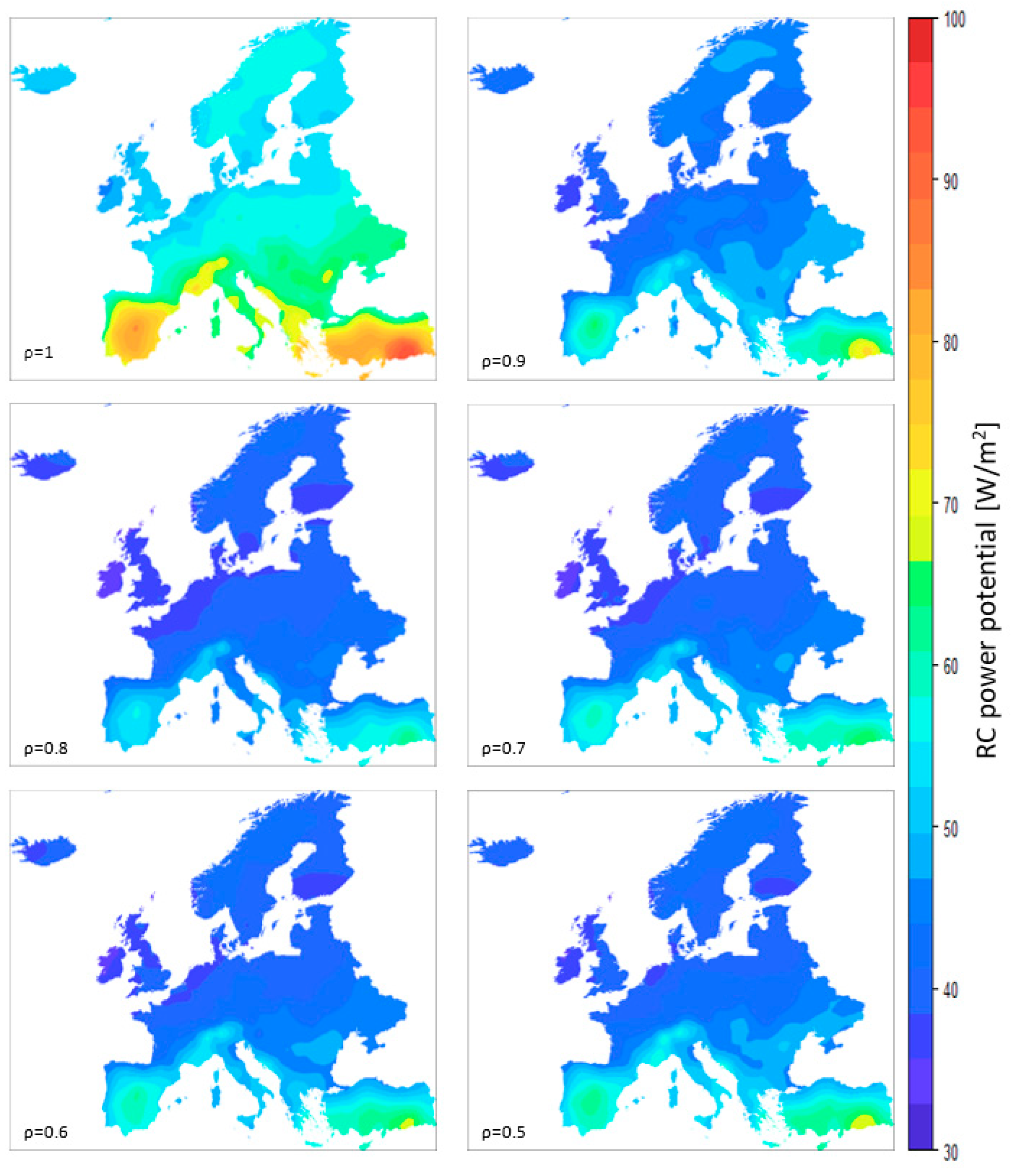
3.2.1. Average Power Potential

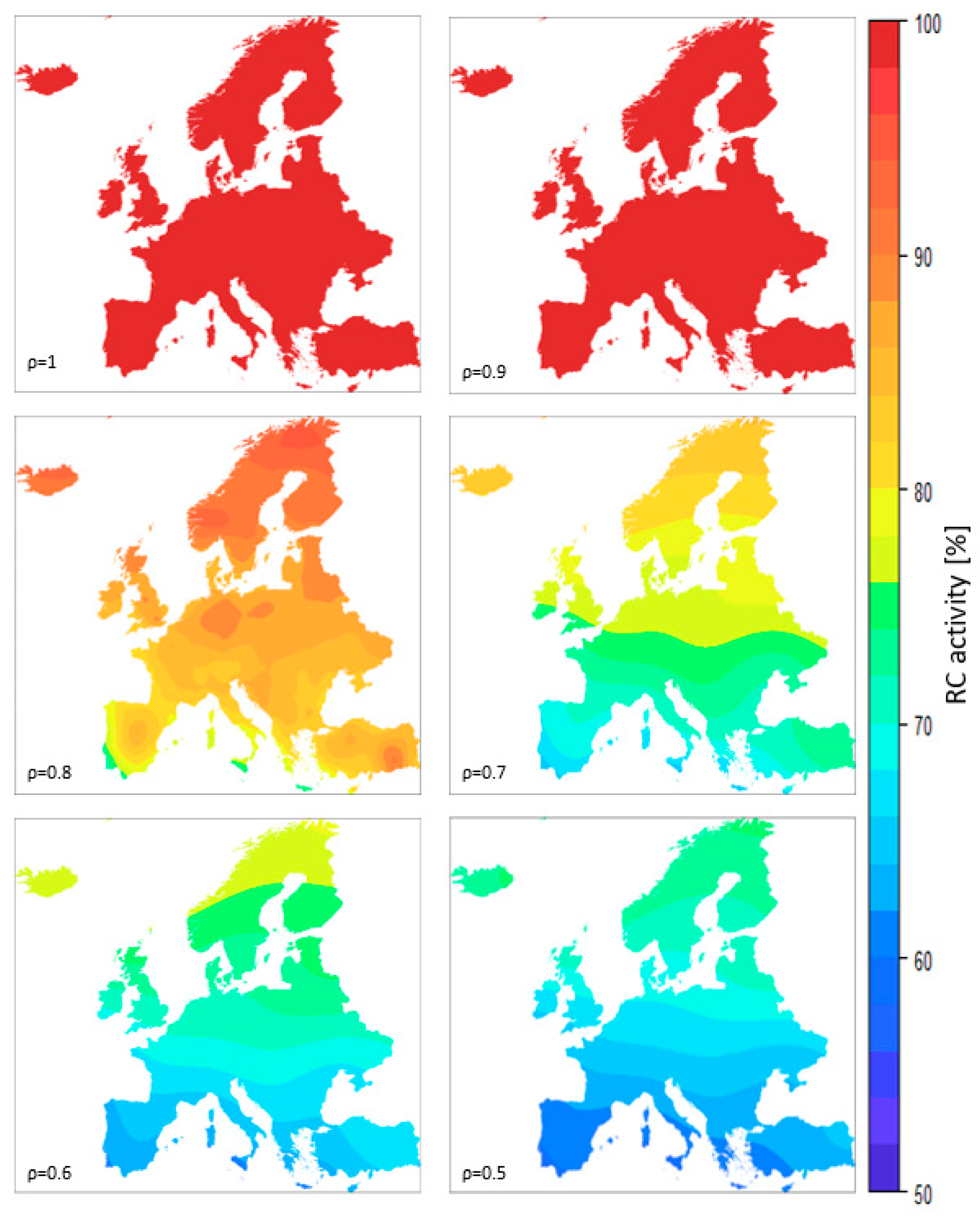
The annual RC power potential maps in Europe are displayed in Figure 4 for each value of reflectivity. The reduction of the reflectivity affects the three regions equally (25% reduction) but, in absolute values, the southern regions are especially penalized (average power reduced by 17.28 W/m²). It is observed that the maps tend to homogenize results throughout the territory as the reflectivity is reduced: the range of values (minimum to maximum average power potential) diminished from 50.19 to 35.05 W/m².

Table 4. Minimum, average and maximum values for each solar reflectivity. Potential maps of RC power (W/m²).

			Solar Reflectivity
	Latitude Range		1	0.9	0.8	0.7	0.6	0.5
Center	43.46 N–53.55 N	min	46.43	36.31	34.20	34.65	35.09	35.82
		avg	58.69	45.27	41.31	42.40	43.34	44.12
		max	73.08	56.17	51.62	53.81	55.98	57.87
North	53.55 N–71.15 N	min	43.82	35.70	33.78	33.55	33.88	34.09
		avg	53.77	43.76	39.31	39.59	39.95	40.23
		max	57.81	48.00	42.19	42.25	42.90	43.38
South	34.60 N–43.46 N	min	56.36	42.23	40.80	42.43	43.67	44.41
		avg	72.33	54.33	49.84	52.51	53.72	55.05
		max	94.01	72.76	62.24	66.05	67.16	69.14
Europe	34.60 N–71.15 N	min	43.82	35.70	33.76	33.55	33.88	34.09
		avg	60.18	46.87	42.61	43.79	44.59	45.32
		max	94.01	72.56	62.34	66.05	67.16	69.14

shows that the average value of the potential of RC power followed a decreasing trend for solar reflectivity from 1 to 0.8, while between 0.7 and 0.5 the potential increased slightly; 0.8 being the value of solar reflectivity where the average potential was minimum (42.61 W/m²). Between 1 and 0.8 a maximum difference of potentials occurred: reducing the solar reflectivity from 1 to 0.8 caused a decrease of 29% in the potential of RC power. Between 0.8 and 0.5, the potential increased 6.4%.

The explanation behind these results is due to the number of observations with which the annual average is calculated. With the reduction of the reflectivity, the total number of RC observations also decreases (see Section 3.2.2). To better understand this, Figure 5 is displayed. The figure shows the power calculated in each of the observations for the month of February at the location of Batman. Observations that resulted in high power values when $\rho$ = 1 remained high when $\rho$ = 0.5, while those observations with low power decreased to the point of having negative values (red points) and were discarded in the calculation of the average. As a result, the calculation of the average for solar reflectivity 0.5 and 0.6 had few observations but of higher quality than for solar reflectivity 0.7 and 0.8. This phenomenon is a result of the different heat fluxes occurring during nighttime and daytime RC. During nighttime RC, solar radiation is not present, thus solar reflectivity does not play any role. However, during daytime RC, solar reflectivity has a significant impact on the radiative balance. In Section 3.2.2. we discuss that most of the observations of RC when considering a solar reflectivity of 0.6 and 0.5 are during nighttime, and thus not affected by this parameter.

We did not observe significant differences in performance of the model for each reflectivity value (

Table 5. Performance of the model of the potential maps of power for different solar reflectivity values.

Reflectivity	R2 (-)	RMSE (W/m2)
1	0.91	2.46
0.9	0.84	2.40
0.8	0.87	1.90
0.7	0.87	2.16
0.6	0.90	2.02
0.5	0.88	2.32

). In all six cases, the values of R² were greater than 0.80 which means that, in all the cases, the models could explain more than 80% of the variability of the sample values. RMSE values were small, indicating that the models had good accuracy.

3.2.2. RC Activity

The maps in Figure 6 show the percentage of hours in a year that the emitter was able to achieve radiative cooling (from now on we refer to this observation of net radiative cooling as “RC activity”). When the reflectivity in the solar range is reduced, the material decreases its behavior as a selective material: when it absorbed more solar radiation the number of observations in which the surface was unable to do radiative cooling increased. In these daytime observations the device was actually behaving as a solar thermal collector, heating up the surface.

Contrary to what the power maps showed, the percentage of RC activity of the emitter decreased as reflectivity decreased in the six cases (

Table 6. Minimum, average and maximum values for each solar reflectivity. RC Activity (%).

			Solar Reflectivity
	Latitude Range		1	0.9	0.8	0.7	0.6	0.5
Center	43.46 N–53.55 N	min	100	100	79.04	68.52	63.76	61.29
		avg	100	99.89	85.68	74.93	69.42	65.93
		max	100	98.55	89.41	78.36	73.07	69.55
North	53.55 N–71.15 N	min	100	99.72	84.34	76.60	70.87	67.07
		avg	100	99.96	90.42	80.53	75.21	71.66
		max	100	99.99	94.48	84.12	78.33	74.53
South	34.60 N–43.46 N	min	100	99.03	72.35	64.03	60.55	58.43
		avg	100	99.78	82.50	70.25	65.08	62.07
		max	100	99.96	90.32	73.37	67.73	64.50
Europe	34.60 N–71.15 N	min	100	98.55	72.35	64.03	60.55	58.43
		avg	100	99.89	86.58	75.78	70.41	67.07
		max	100	100	94.48	84.12	78.33	74.53

). For a reflectivity of 0.5, the worst-case scenario, only in 67% of cases was radiative cooling achieved; the remaining 33% were solar collection observations. Northern regions had more observations of radiative cooling, in all the cases, which means more time available to perform radiative cooling, than southern regions. In Section 3.1 it was pointed out that nighttime RC represented 59.6% of the RC activity in Europe, this means that only 7.47% of the activity occurred during daytime when $\rho =0.5$; 10.81%, when $\rho =0.6$; 16.18%, when $\rho =0.7;$ 26.98%, when $\rho =0.8;$ 40.29%, when $\rho =0.9$ and 40.4%, when $\rho =1$.

The results of RC activity for $\rho$ = 1 have not been interpolated by Kriging as a variability in the values to be interpolated is required. For this case, all values were equal to 100% and Kriging could not be performed. It was assumed that in unknown locations the RC activity value was 100%.

The model for reflectivity 0.9 showed a low R² value and low RMSE. This model could not reproduce much of the variability of the sample but it also gives low errors of prediction. The range of the values of the sample was very small. For reflectivity values below 0.9, the models presented good metrics of R² and RMSE (

Table 7. Performance of the model of the potential maps of RC activity for different solar reflectivity values.

Reflectivity	R2 (-)	RMSE (-)
0.9	0.25	0.19
0.8	0.84	1.49
0.7	0.87	1.43
0.6	0.88	1.24
0.5	0.91	1.05

).

3.2.3. Annual Energy Potential

The maps in Figure 7 show the annual RC energy potential at each point in Europe. It can be seen, again, that the regions of southern Europe are the areas with the highest energy capacity for radiative cooling. For solar reflectivity values between 0.8 and 0.6, northern regions present higher energy potential than central regions. In this range, although the power potential in the north was lower than in the center (Figure 4 and Figure 5), the north had more time available to perform RC (Figure 6 and Table 6), resulting in higher values of annual energy available.

The available energy was reduced by lowering solar reflectivity (

Table 8. Minimum, average and maximum values for each solar reflectivity. Potential maps of annual RC energy (kWh/m²·year).

			Solar Reflectivity
	latitude Range		1	0.9	0.8	0.7	0.6	0.5
Center	43.46 N–53.55 N	min	406.74	312.63	254.79	228.15	220.30	213.05
		avg	514.16	396.23	309.89	278.54	263.55	254.74
		max	639.71	493.03	378.74	333.92	322.46	317.90
North	53.55 N–71.15 N	min	384.08	313.42	258.55	232.97	221.06	213.08
		avg	470.99	383.47	311.62	280.07	264.03	253.50
		max	506.40	422.26	346.71	309.46	291.11	278.34
South	34.60 N–43.46 N	min	493.88	368.86	281.38	266.07	246.96	240.26
		avg	633.56	475.55	360.98	323.36	306.98	299.93
		max	822.66	642.35	492.60	413.61	397.85	388.09
Europe	34.60 N–71.15 N	min	384.08	312.63	254.79	228.15	220.30	213.05
		avg	527.10	410.35	322.43	289.55	273.87	264.87
		max	822.66	642.35	492.60	413.61	397.85	388.09

). At low reflectivities, maps presented a homogenization pattern. When solar reflectivity is equal to 0.5 it behaves as a nighttime surface (when $\rho$ = 0.5 it was able to provide, on average, 264.87 kWh/m²·year, while a nighttime surface was able to provide 245.76 kWh/m²·year). The largest differences in the average annual RC energy were observed between $\rho$ = 1 and $\rho$ = 0.8. In this range, the difference between average values in Europe was equal to 204.67 kWh/m²·year, and it was equal to 272.58 kWh/m²·year in southern Europe. In the range of 0.8–0.5, the existing difference in the average was equal to 57.56 kWh/m²·year in Europe. Between $\rho$ = 1 and $\rho$ = 0.8, the average annual RC energy reduction for Europe was 38.83%, while between $\rho$ = 0.8 and $\rho$ = 0.5 it was 17.85%. Small variations in reflectivity have a greater impact on the energy potential at high reflectivity values than at low ones.

Southern countries were more affected by the reduction of $\rho$ than northern and central countries: differences in the average RC energy available between $\rho$ = 1 and $\rho$ = 0.5 were 333.63 kWh/m²·year in southern regions, 259.42 kWh/m²·year in central regions and 217.49 kWh/m²·year in northern regions. The model presented a good performance in the six cases (

Table 9. Performance of the model of the potential maps of RC energy for different solar reflectivity values.

Reflectivity	R2 (-)	RMSE (kWh/m2·year)
1	0.91	21.58
0.9	0.83	21.34
0.8	0.81	16.24
0.7	0.74	16.04
0.6	0.81	13.30
0.5	0.78	13.82

).

4. Conclusions

In this article we presented the potential of implementing nighttime and all-day radiative cooling technologies in Europe for different solar reflectivity values of the RC emitting surface. Based on climatological data from weather stations and using Kriging interpolation techniques, maps of annual potential for RC power, RC energy and RC activity were displayed. The following conclusions can be drawn from the study:

• Kriging is a good methodology to predict radiative cooling values from known climatological data. The models presented high values of R² and low values of RMSE.
• With the implementation of new materials, all-day radiative cooling can be achieved. For solar reflectivity equal to 1, the shift from nocturnal to all-day radiative cooling can improve the average potential power from 47.30 to 60.17 W/m², with peak values of 94.01 W/m². The average annual energy increases from 245.76 to 559.47 kWh/m²·year.
• The areas with the greatest potential of implementation are the regions of southern Europe. These regions present high values of power and energy potential.
• Compared to the other regions, the north holds more hours of available radiative cooling.
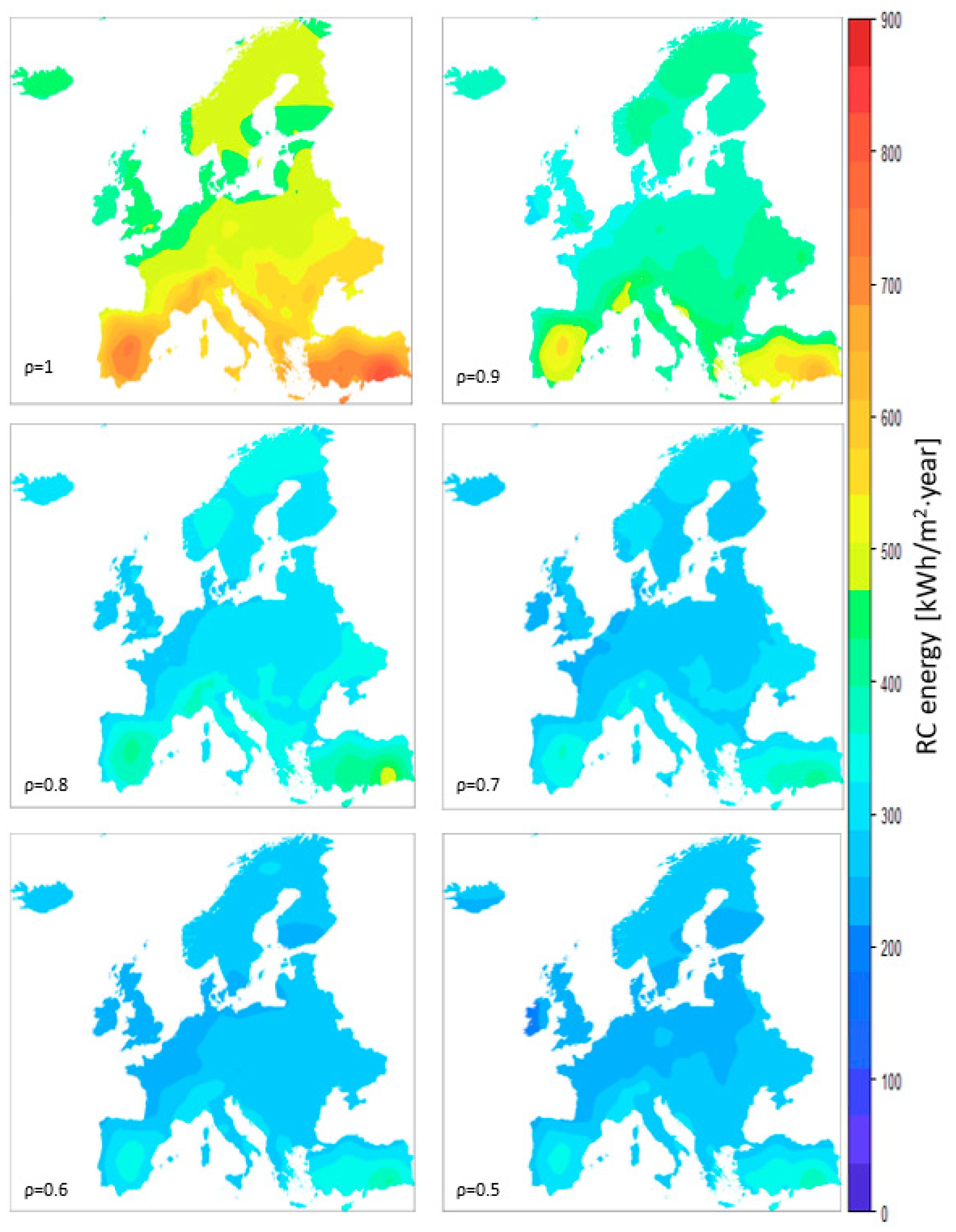
• The best performance, in all the three regions defined, is achieved when solar reflectivity is equal to one. In order to minimize the solar radiation absorbed by the surface, the reflectivity values in the solar range must be close to 1.
• For solar reflectivity values below 0.5, the behavior of the surface can be assimilated to a nighttime radiative cooler.
• Annual energy and RC activity decreases with reflectivity, while average power potential presents higher values in the 0.6–0.5 range for reflectivity, rather than in the 0.8–0.7 range. This is a result of calculating the average powers using only the observations where RC is achieved, and not for all the observations; for low solar reflectivity values, RC observations correspond mainly to nighttime values where high-power values are obtained. On the contrary, for solar reflectivity values between 0.8 and 0.7, the same nocturnal RC values are achieved, as well as a higher number of low-power daytime observations, thus reducing the average power. Finally, when the solar reflectivity is equal to 0.9, diurnal observations present higher powers, thus increasing the average power.
• For low values of solar reflectivity, maps tend to show homogeneous patterns.
• Small variations in solar reflectivity have greater impacts on the potential at higher reflectivity values than lower ones: in the range of 1–0.8, the reduction of average power potential is 29.19% and the annual energy is 38.83%.

References

1. Bahadori, M.N. Passive Cooling Systems in Iranian Architecture. Sci. Am. 1978, 238, 144–155. [Google Scholar] [CrossRef]
2. Johnson, T.E. Radiation Cooling of Structures with Infrared Transparent Wind Screens. Sol. Energy 1975, 17, 173–178. [Google Scholar] [CrossRef]
3. Catalanotti, S.; Cuomo, V.; Piro, G.; Ruggi, D.; Silvestrini, V.; Troise, G. The Radiative Cooling of Selective Surfaces. Sol. Energy 1975, 17, 83–89. [Google Scholar] [CrossRef]
4. Vall, S.; Johannes, K.; David, D.; Castell, A. A New Flat-Plate Radiative Cooling and Solar Collector Numerical Model: Evaluation and Metamodeling. Energy 2020, 202, 117750. [Google Scholar] [CrossRef]
5. Sodha, M.S.; Singh, U.; Tiwari, G.N. A Thermal Model of a Roof Pond System with Moveable Insulation for Heating a Building. Build. Environ. 1982, 17, 135–144. [Google Scholar] [CrossRef]
6. Raman, A.P.; Anoma, M.A.; Zhu, L.; Rephaeli, E.; Fan, S. Passive Radiative Cooling below Ambient Air Temperature under Direct Sunlight. Nature 2014, 515, 540–544. [Google Scholar] [CrossRef]
7. Cunha, N.F.; AL-Rjoub, A.; Rebouta, L.; Vieira, L.G.; Lanceros-Mendez, S. Multilayer Passive Radiative Selective Cooling Coating Based on Al/SiO2/SiNx/SiO2/TiO2/SiO2 Prepared by Dc Magnetron Sputtering. Thin Solid Film. 2020, 694, 137736. [Google Scholar] [CrossRef]
8. Kecebas, M.A.; Menguc, M.P.; Kosar, A.; Sendur, K. Passive Radiative Cooling Design with Broadband Optical Thin-Film Filters. J. Quant. Spectrosc. Radiat. Transf. 2017, 198, 179–186. [Google Scholar] [CrossRef]
9. Mandal, J.; Fu, Y.; Overvig, A.C.; Jia, M.; Sun, K.; Shi, N.N.; Zhou, H.; Xiao, X.; Yu, N.; Yang, Y. Hierarchically Porous Polymer Coatings for Highly Efficient Passive Daytime Radiative Cooling. Science 2018, 362, 315–319. [Google Scholar] [CrossRef] [PubMed] [Green Version]
10. Peng, L.; Liu, D.; Cheng, H. Design and Fabrication of the Ultrathin Metallic Film Based Infrared Selective Radiator. Sol. Energy Mater. Sol. Cells 2019, 193, 7–12. [Google Scholar] [CrossRef]
11. Zhang, J.; Zhou, Z.; Quan, J.; Zhang, D.; Sui, J.; Yu, J.; Liu, J. A Flexible Film to Block Solar Radiation for Daytime Radiative Cooling. Sol. Energy Mater. Sol. Cells 2021, 225, 111029. [Google Scholar] [CrossRef]
12. Bao, H.; Yan, C.; Wang, B.; Fang, X.; Zhao, C.Y.; Ruan, X. Double-Layer Nanoparticle-Based Coatings for Efficient Terrestrial Radiative Cooling. Sol. Energy Mater. Sol. Cells 2017, 168, 78–84. [Google Scholar] [CrossRef]
13. Hossain, M.M.; Jia, B.; Gu, M. A Metamaterial Emitter for Highly Efficient Radiative Cooling. Adv. Opt. Mater. 2015, 3, 1047–1051. [Google Scholar] [CrossRef]
14. Zhai, Y.; Ma, Y.; David, S.N.; Zhao, D.; Lou, R.; Tan, G.; Yang, R.; Yin, X. Scalable-Manufactured Randomized Glass-Polymer Hybrid Metamaterial for Daytime Radiative Cooling. Science 2017, 355, 1062–1066. [Google Scholar] [CrossRef] [PubMed] [Green Version]
15. Cho, J.-W.; Lee, T.-I.; Kim, D.-S.; Park, K.-H.; Kim, Y.-S.; Kim, S.-K. Visible to Near-Infrared Thermal Radiation from Nanostructured Tungsten Anntennas. J. Opt. 2018, 20, 09LT01. [Google Scholar] [CrossRef]
16. Wu, D.; Liu, C.; Xu, Z.; Liu, Y.; Yu, Z.; Yu, L.; Chen, L.; Li, R.; Ma, R.; Ye, H. The Design of Ultra-Broadband Selective near-Perfect Absorber Based on Photonic Structures to Achieve near-Ideal Daytime Radiative Cooling. Mater. Des. 2018, 139, 104–111. [Google Scholar] [CrossRef]
17. Rephaeli, E.; Raman, A.; Fan, S. Ultrabroadband Photonic Structures to Achieve High-Performance Daytime Radiative Cooling. Nano Lett. 2013, 13, 1457–1461. [Google Scholar] [CrossRef]
18. Zhu, L.; Raman, A.P.; Fan, S. Radiative Cooling of Solar Absorbers Using a Visibly Transparent Photonic Crystal Thermal Blackbody. Proc. Natl. Acad. Sci. USA 2015, 112, 12282–12287. [Google Scholar] [CrossRef] [Green Version]
19. Gao, M.; Han, X.; Chen, F.; Zhou, W.; Liu, P.; Shan, Y.; Chen, Y.; Li, J.; Zhang, R.; Wang, S.; et al. Approach to Fabricating High-Performance Cooler with near-Ideal Emissive Spectrum for above-Ambient Air Temperature Radiative Cooling. Sol. Energy Mater. Sol. Cells 2019, 200, 110013. [Google Scholar] [CrossRef]
20. Vall, S.; Castell, A.; Medrano, M. Energy Savings Potential of a Novel Radiative Cooling and Solar Thermal Collection Concept in Buildings for Various World Climates. Energy Technol. 2018, 6, 2200–2209. [Google Scholar] [CrossRef]
21. Feng, J.; Santamouris, M.; Shah, K.W.; Ranzi, G. Thermal Analysis in Daytime Radiative Cooling. IOP Conf. Ser. Mater. Sci. Eng. 2019, 609, 072064. [Google Scholar] [CrossRef]
22. Bijarniya, J.P.; Sarkar, J.; Maiti, P. Environmental Effect on the Performance of Passive Daytime Photonic Radiative Cooling and Building Energy-Saving Potential. J. Clean. Prod. 2020, 274, 123119. [Google Scholar] [CrossRef]
23. Carlosena, L.; Ruiz-Pardo, Á.; Feng, J.; Irulegi, O.; Hernández-Minguillón, R.J.; Santamouris, M. On the Energy Potential of Daytime Radiative Cooling for Urban Heat Island Mitigation. Sol. Energy 2020, 208, 430–444. [Google Scholar] [CrossRef]
24. Argiriou, A.; Santamouris, M.; Balaras, C.; Jeter, S. Potential of Radiative Cooling in Southern Europe. Int. J. Sol. Energy 1992, 13, 189–203. [Google Scholar] [CrossRef]
25. Chang, K.; Zhang, Q. Modeling of Downward Longwave Radiation and Radiative Cooling Potential in China. J. Renew. Sustain. Energy 2019, 11, 066501. [Google Scholar] [CrossRef]
26. Li, M.; Peterson, H.B.; Coimbra, C.F.M. Radiative Cooling Resource Maps for the Contiguous United States. J. Renew. Sustain. Energy 2019, 11, 036501. [Google Scholar] [CrossRef]
27. Aubinet, M. Longwave Sky Radiation Parametrizations. Sol. Energy 1994, 53, 147–154. [Google Scholar] [CrossRef]
28. Hengl, T. A Practical Guide to Geostatistical Mapping. 2019, p. 15. Available online: http://spatial-analyst.net/book/system/files/Hengl_2009_GEOSTATe2c1w.pdf (accessed on 19 August 2021).
Figure 1. Spatial distribution of the sample points.
Atmosphere 12 01119 g001
Figure 2. Map of annual average power potential (W/m2) of nighttime RC (left) and all-day RC of an ideal solar reflective surface (right). Horizontal red lines divide the map into three zones: north (53.55 N–71.15 N), center (43.46 N–53.55 N) and south (34.60 N–43.46 N).
Atmosphere 12 01119 g002
Figure 3. Map of annual energy potential (kWh/m2·year) of nighttime RC (left) and all-day RC of an ideal solar reflective surface (right). Horizontal red lines divide the map into three zones: north (53.55 N–71.15 N), center (43.46 N–53.55 N) and south (34.60 N–43.46 N).
Atmosphere 12 01119 g003
Figure 4. Map of RC power potential (W/m2) for six values of solar radiation reflectivity.
Atmosphere 12 01119 g004
Figure 5. Power potential for each observation in Batman during the month of February and for each value of solar reflectivity. Blue points correspond to radiative cooling observations and red points correspond to solar heating observations. Red observations were discarded in calculations.
Atmosphere 12 01119 g005
Figure 6. Map of RC activity (%) for six values of solar radiation reflectivity.
Atmosphere 12 01119 g006
Figure 7. Map of annual RC energy (kWh/m2·year) for six values of solar radiation reflectivity.
Atmosphere 12 01119 g007