Article

WRF-Chem Modeling of Summertime Air Pollution in the Northern Great Plains: Chemistry and Aerosol Mechanism Intercomparison

by
Carlos J. Bucaram
* and
Frank M. Bowman
*
Department of Chemical Engineering, University of North Dakota, 243 Centennial Dr., Grand Forks, ND 58202-7101, USA
*
Authors to whom correspondence should be addressed.
Atmosphere 2021, 12(9), 1121; https://doi.org/10.3390/atmos12091121
Submission received: 14 July 2021 / Revised: 12 August 2021 / Accepted: 27 August 2021 / Published: 31 August 2021
(This article belongs to the Section Air Quality)

Abstract

:
Oil and gas production in the Bakken region increased dramatically during the past decade. A WRF-Chem modeling study of the Northern Great Plains was conducted for a July 2010 baseline scenario prior to the largest of these production increases. Simulations using the RACM-MADE/SORGAM, CBMZ-MOSAIC, and MOZART-MOSAIC chemistry-aerosol mechanisms were compared to each other and against ground level observations. All three gas-aerosol modules produced similar prediction results for O3, and NO2, with moderate correlation to hourly measurements and monthly average values overpredicted by 20% for O3 and underpredicted by 5% for NO2. Monthly average PM2.5 concentrations were relatively accurate, but correlation to hourly measurements was very low and PM2.5 subspecies exhibited high variability with a mix of over and underpredictions depending on the mechanism. Pollutant concentrations were relatively low across the mostly rural study domain, especially in the Bakken region. Results from this work can be used as a basis of comparison for studies of more recent time periods that include increased oil and gas-related emissions.

1. Introduction

Oil and gas production activities have increased considerably in the United States over the last decade, which has caused increased volatile organic compound (VOC) and nitrogen oxide (NOx) air pollutant emissions [1]. One area that has seen dramatic changes is the Bakken oil region, which spans 520,000 km2 across western North Dakota and eastern Montana in the U.S., as well as southwestern Manitoba and southeastern Saskatchewan in Canada [2]. Drilling activity in the Bakken region increased ten-fold between 2007 and 2015 and has since maintained an average production rate of over 1.1 million barrels a day, now making North Dakota (ND) the second largest oil-producing state in the U.S. During the same time, natural gas production has also increased more than ten-fold [3]. Monitoring data in the Bakken region has shown corresponding increases in atmospheric levels of NOx, VOCs, and PM2.5 [2,4,5,6,7].
Atmospheric modeling can provide further insight into these changes and can help predict future impacts of continued drilling activities and increases in production. Modeling of the Bakken region, however, has been limited, with no modeling studies focused specifically on the Northern Great Plains (NGP). Simulations of the broader continental U.S. offer some general information on recent and potential future pollutant conditions of relevance to the Northern Great Plains region. Simulations of air quality in the western half of the U.S. in 2011 with and without oil and gas emissions showed widespread impacts on O3 and nitrogen deposition, and more localized contributions to PM2.5 and visibility [8]. For the modeled 2011 scenario, impacts on the Bakken region were small, consistent with lower oil and gas emissions at that time relative to other areas of the country, as oil and gas activity in North Dakota was just beginning its dramatic increase. Modeling of ozone and PM trends from 1970 to 2020 showed that O3 and PM2.5 levels have been decreasing across the United States, consistent with NOx, VOC, and PM emission reductions [9]. At the same time, background O3, attributable to natural sources and anthropogenic emissions outside the U.S., has slowly increased. The influence of background O3 is more pronounced in the western half of the U.S., and is most evident in rural areas, with fewer local emission sources. For ND in 2020, background sources are estimated to account for 80–90% of total average peak O3 levels of 45–55 ppb. These simulations include some projections of future oil and gas emissions, but may not account for all of the recent emission increases occurring in the Bakken.
Simulations of the continental U.S. during the 2001–2010 period generally agree with measurement data showing pollutant concentrations in the Bakken region to be relatively low [10,11]. Annual average O3 levels are approximately 30 ppb and annual average PM2.5 concentrations are approximately 4 μg/m3. Simulations for 2050 predict O3 in the Bakken to increase or decrease by 2–3 ppb, depending on the representative concentration pathway (RCP) emission scenario used, and PM2.5 to decrease by 2–3 μg/m3 [12]. These simulations and associated model validation are based on the entire continental U.S., leaving unclear how well they perform for the Northern Great Plains specifically. Again, the future year simulations do not account for recent and potential future increases in oil and gas development activity. To better assess oil and gas impacts in the Bakken region, accurate baseline modeling of the NGP is needed.
Accuracy of model predictions is dependent on the accuracy of model inputs (emissions, boundary conditions, etc.) [13,14,15] and on the model formulations used to represent physical and chemical processes (transport, gas phase chemistry, aerosol dynamics and chemistry) [16,17,18,19,20]. A variety of chemical transport models are currently available, e.g., [21,22,23,24,25]. One of the most widely used is WRF-Chem, which couples gas and aerosol chemistry, emissions, and transport with meteorology. Options for gas-phase chemical mechanisms within WRF-Chem include CBM-Z [26], CBM-IV [27], RADM2 [28], RACM [29], SAPRC-99 [30], and MOZART [31]. Available aerosol schemes include MOSAIC [32], MADE/SORGAM [33,34], MADE/VBS [33,35], MAM [36], and GOCART [37].
WRF-Chem model performance has been evaluated in numerous studies [11,17,20,38,39,40,41,42,43]. For gas phase chemistry, the mechanisms generally agree with each other and perform reasonably well at predicting concentrations of O3, CO, and NO2, with normalized mean bias (NMB) less than 20% [17,44,45,46,47]. Predictions of radical and intermediate gas-phase species such as OH, HO2, NO3, and HCHO show larger errors and variation between mechanisms. For aerosol phase predictions, many models are able to produce PM2.5 results with NMB less than 20%, but often this is a result of offsetting errors in component concentrations where, for example, organic aerosol is underpredicted, but sulfate is overpredicted [10,44]. Moreover, while model performance averaged across an entire domain may be good, it may vary between subregions and in some locations, such as urban areas and more complex terrain, in which performance may be poorer [12,20,41]. Therefore, it is important that model evaluation consider the specific location and scenario of interest to ensure an appropriate model formulation is being used to properly interpret simulation results.
In this paper, we provide a comparison of three WRF-Chem chemistry-aerosol modules for baseline simulations of the NGP in July 2010 prior to the recent oil boom. WRF-Chem predictions of meteorological variables and gas and aerosol phase pollutant concentrations using the chemistry-aerosol packages CMBZ-MOSAIC, RACM-MADE/SORGAM, and MOZART-MOSAIC were compared to each other and against ground-level observations. The model domain uses a 24 km resolution to cover parts of seven states in the Northern Great Plains, providing the first modeling study, to our knowledge, specifically focused in this geographical area. July 2010 was used as a representative summertime episode, the season when ozone and PM2.5 pollutant levels have historically been highest [48], at a time when oil and gas production activities in the region were still small relative to current and expected future activity. The aims of this work were to identify an appropriate combination of model options for simulating this region and use them in a simulation reflecting baseline conditions within our region of study. The results of these baseline model simulations will be used as a basis of comparison for future studies assessing the impact of oil and gas-related activities on regional air quality.

2. Methods

2.1. Model Configuration

The WRF-Chem model, version 3.8 [22,49], was used for this research work. Gas-phase chemistry and aerosol chemistry and physics were represented with three chemistry-aerosol modules, namely MOZART-MOSAIC [31,32], CBMZ-MOSAIC [26,32], and RACM-MADE/SORGAM [29,33,34], These three chemistry-aerosol mechanisms have been extensively studied, with researchers reporting acceptable results under a wide variety of set-up conditions [11,17,20,35,41].
The Model of Ozone and Related Chemical Tracers (MOZART) [31] gas-phase chemistry mechanism includes 85 chemical species and 196 reactions. MOZART is coupled with the Model for Simulating Aerosol Interactions and Chemistry (MOSAIC) [32] aerosol scheme, using four sectional size bins to reduce computational cost. The MOZART-MOSAIC (MM) scheme used includes a limited set of secondary organic aerosol (SOA) species. The Zaveri version of the Carbon Bond Mechanism (CBMZ) gas-phase chemistry mechanism [26] is based on the Carbon Bond Mechanism (CBM-IV) [27] and includes 52 total species and 132 reactions. CBMZ is also coupled with MOSAIC. SOA is not included in the CBMZ-MOSAIC (CM) scheme used in this study. The Regional Atmospheric Chemistry Mechanism (RACM) [29] includes 77 gas-phase species and 237 reactions. In this work, the RACM mechanism was coupled with the Modal Aerosol Dynamics Model for Europe (MADE) [33], which describes the aerosol with 3 log-normal modes. A limited number of secondary organic aerosol species were incorporated into MADE with the Secondary Organic Aerosol Model (SORGAM) [34]. RACM chemical mechanism code for implementation in WRF-Chem was generated with the kinetic preprocessor (KPP) [50,51]. The main physical and chemical parameterizations used in WRF-Chem are shown in Table 1. A 24 km grid resolution with 28 vertical layers was used to achieve a balance of accuracy and computational cost. A common set of meteorological and physical options in WRF-Chem were used for simulations with the three different chemistry-aerosol schemes.

2.2. Model Scenario

The model scenario used in this study is a simulation of July 2010 in the Northern Great Plains. As shown in Figure 1, the modeling domain included all of the central United States, with analysis focused on the region surrounding and downwind of the Bakken oil formation. The analysis region, indicated by the red box in Figure 1, included the states of North Dakota, South Dakota, Nebraska, Montana, Wyoming, Minnesota, and Iowa. This largely excluded population and pollution sources in the surrounding areas so that analysis could focus on this more rural and unpolluted region. Data from North Dakota monitoring sites showed an O3 concentrations peak during the summer, while PM2.5 concentrations showed no seasonal trend and remained constant on average throughout the year [48,58]. July was used to represent these summertime conditions when both O3 and PM2.5 concentrations in North Dakota are the highest. The 2010 year was selected because it had meteorological conditions, similar to average conditions during the past decade. Additionally, importantly, in 2010 oil and gas production was relatively low (0.3 million barrels oil per day in 2010, compared with over 1.1 million barrels per day each year since 2014 [59]), providing a baseline scenario of the region before the subsequent increases in oil and gas development and associated emissions.
The meteorological input data sets for the year 2010 were downloaded from the North American Regional Reanalysis (NARR) 3-h data, at 32 km resolution [60]. Model input data for the emitted chemical species used hourly area and point source anthropogenic emissions from the 2011 National Emission Inventory (NEI-2011) [61] at 4 km resolution, and biogenic emissions from the MEGAN 2.04 model [62] at 1 km resolution. The NEI-2011 emissions include hourly emissions data for an average July weekday that is used to represent emission rates on all days of a simulation. Biogenic emissions vary throughout the month based on simulated hourly temperature and solar radiation. Initial and lateral boundary conditions for chemical species were obtained from the MOZART-4 model [31]. MOZART output data at 6-h intervals was downloaded from the National Center for Atmospheric Research (NCAR) [63] and then converted to the proper format for WRF-Chem using the MOZBC pre-processor [64].
To ensure that simulation results did not drift significantly from real meteorological conditions, the month-long scenario was simulated in 5-day intervals [41]. A 12-h meteorological spin up was used before each 5-day interval and a 5-day spin up time was used to initialize the entire scenario. Some of the simulations were carried out on a high-performance computing system consisting of 3.3GHz Intel Xeon E5-2643 processors(Intel: Santa Clara, CA, USA) with a 56 Gbit EDR InfiniBand (IB) interconnect and a GPFS parallel file system. Every 5.5 meteorological day model run took about 13 h to complete using 8 cores of this HPC system. Other simulations were carried out on an individual Linux PC consisting of a 3.4–4.0 GHz, 4-core Intel Core i7-6700 Processor (Intel: Santa Clara, CA, USA). Every 5.5 meteorological day model run took about 84 h to complete using this PC system.

2.3. Observational Data and Analysis

Model predictions were compared to ground level observational data for July 2010 from EPA’s Chemical Speciation Network (CSN) [58], Clean Air Status and Trends Network [65], and the Interagency Monitoring of Protected Visual Environments (IMPROVE) network [66]. Locations of the monitoring sites are shown in Figure 1. There were a total of 47 sites reporting data for one or more of the following: hourly values of O3 (27 sites), NO2 (10), PM2.5 (18), near-ground temperature at 2 m (15), surface pressure (9), relative humidity (12), wind speed at 10 m (6), and 24-h values every third day for PM2.5 components OC (15), EC (15), SO42− (22), NO3 (21), and NH4 (6). Additional details for each of the monitoring sites are found in Table S1 of the Supplementary Information. Sites were assigned into a western group that includes the Bakken and an eastern group, mainly in or near Minnesota and Iowa.
Statistical analysis was performed comparing CBMZ-MOSAIC, RACM-MADE/SORGAM, and MOZART-MOSAIC model predictions to the observational data. Reported statistical measures include Pearson’s correlation coefficient (R), mean bias (MB), normalized mean bias (NMB), and root mean square error (RMSE), which are defined in Table 2. Only monitoring sites with <10% missing data were included in the analysis. For aerosol components, the modeled PM2.5 subspecies mass concentration was determined by adding the first three size bins of the MOSAIC scheme or the Aitken and accumulation modes of the MADE/SORGAM aerosol scheme. For organic carbon (OC), RACM-MADE/SORGAM model predictions of organic aerosol (OA) were divided by a factor of 1.4 to obtain OC values, consistent with a commonly used OA:OC ratio [67].

3. Results and Discussion

3.1. Meteorology

July 2010 exhibited typical summer weather conditions across the study domain. Daily high temperatures were generally 25–35 °C and nighttime lows were 10–20 °C. Scattered rainfall was present somewhere within the region on most days and several periods of strong thunderstorms occurred, most notably 4, 22–24 and 27–28 July. Total monthly precipitation varied from 2–10 cm in the western half of the study region to 10–30 cm in the east, with the highest totals in the southeast [68].
In recent years, the study domain has periodically been impacted by heavy smoke events produced by wildfires in the western United States and Canada. MODIS/Terra satellite imagery for early July 2010 show a cluster of large fires in northern Saskatchewan with clearly visible smoke plumes. On most days, smoke from these fires remained in Canada, north of the model domain for this study, with the only exception on July 15 when there appeared to be a smoke event across parts of ND and into Minnesota [69].
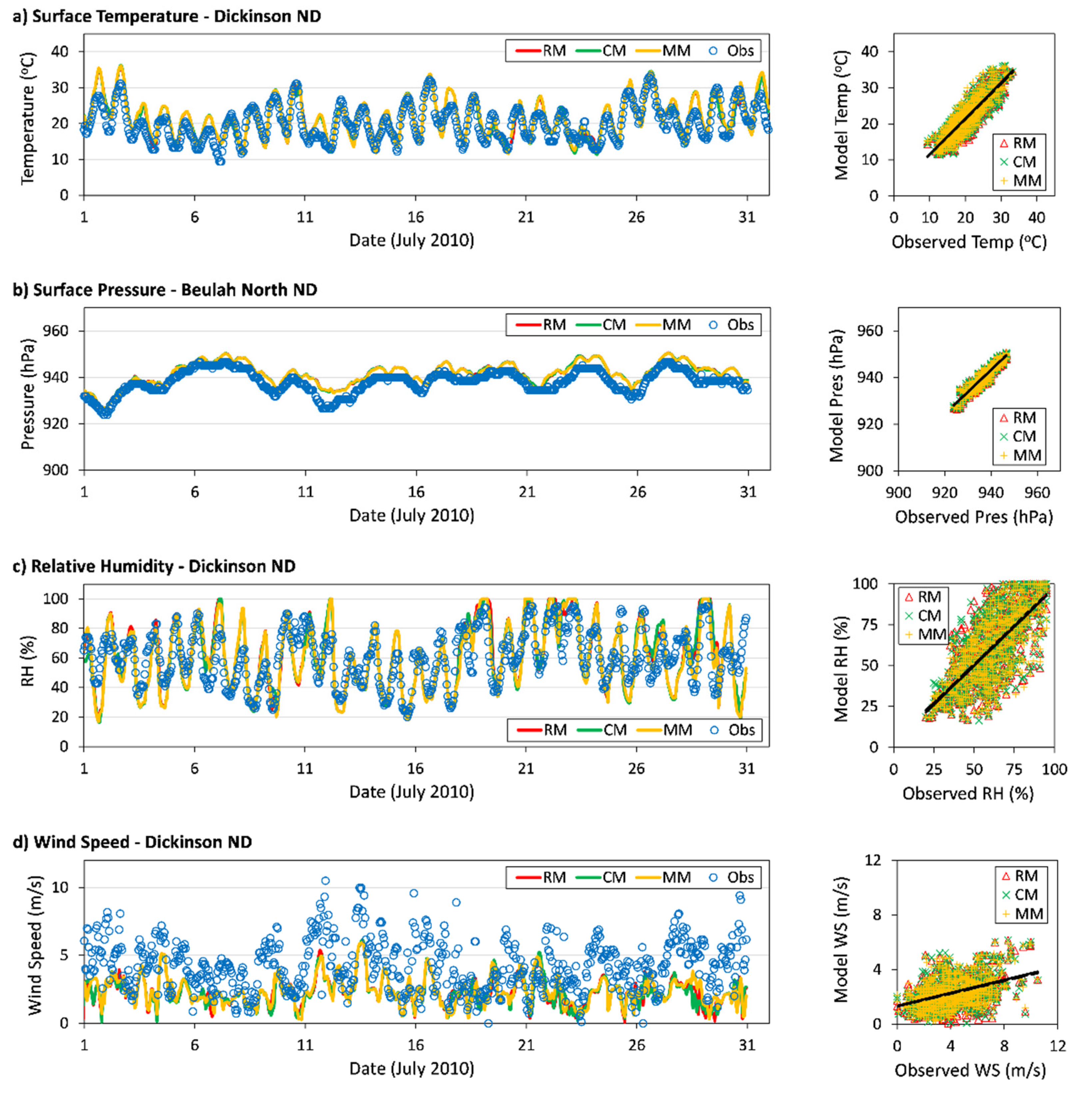
Table 3 lists averaged statistical results comparing meteorological predictions from simulations with the RACM-MADE/SORGAM (RM), CBMZ-MOSAIC (CM), and the MO-ZART-MOSAIC (MM) chemistry-aerosol mechanisms to measurements at ground stations across the domain area of study. These and other statistical results reported for this study are averages of the measures determined for individual stations. A summary of the statistical measures at each location is provided in Tables S2–S5 in the Supplementary Materials. For near-ground temperature and surface pressure, all three models produced similar results that agree well on average with observations, as evidenced by average NMB values of approximately 2% and −0.3%, and average Pearson’s correlation coefficients of 0.80 and 0.92, respectively. The models all showed only a small underprediction of average near-ground relative humidity, with −4% average NMB, but produced somewhat lower correlation to hourly observations (average R-value of 0.67). For 10 m wind speed, the three models did not perform quite as strongly, with a tendency toward somewhat larger overpredictions (average NMB value of 30%) and only moderate correlations with observations (average R-value of 0.48). These results are comparable to other studies with WRF-Chem where wind speed was overpredicted by 30–100% [44,70,71]. Differences in meteorological results between the three model formulations was minimal, with only slight variation in the average statistical measures. This is not surprising because the three chemistry-aerosol mechanisms are coupled to the same base WRF meteorological model. The simulations did not produce identical meteorological results to each other because aerosol-cloud-radiation feedbacks in the coupled WRF-Chem model are influenced differently by the different aerosol and gas chemistry mechanism formulations.
The effect of geographical location was explored by comparing meteorological parameters for eastern and western monitoring sites. Western sites had lower average observed temperature (20.7 °C in the west vs. 24 °C in the east) possibly due to western sites generally being further north, lower pressure (941 vs. 981 hPa) due to higher elevations in the west, much lower RH (59% vs. 84%), and higher wind speed (3.5 vs. 2.1 m/s). Statistical performance of the models showed variation between eastern and western sites that was generally small, and the three models continued to be in close agreement with each other. Only wind speed predictions had significant geographical bias, with eastern sites overpredicted on average by 58% and western sites underpredicted by 21% (Table S5, Supplementary Materials).
Simulation results also showed similar performance when looking at diurnal cycles in these meteorological measures. As seen in Figure 2, which shows hourly time series and scatterplots for the Dickinson and Beulah sites in western ND, temperature and pressure predictions correlated well with each other and with ambient measurements. Wind speed and relative humidity predictions aligned less closely with observations, but still captured the hourly variability in these measures reasonably well. The trends shown in Figure 2 for temperature, pressure, and relative humidity are representative of model performance at the other monitoring sites across the modeling domain. Wind speed results in Figure 2 are for a western site with large underpredictions, unlike other sites that showed overpredictions for wind speed. Overall, these results give confidence that the meteorological parameters upon which the chemistry simulations are based were simulated appropriately.

3.2. Ozone

Model predictions of maximum hourly O3 concentrations are shown in Figure 3 for the RM, CM, and MM chemistry-aerosol mechanisms. The models were generally similar to each other; all three showed a pattern of highest maximum O3 concentrations where major cities are located and towards the southwest and southeast. Peak concentrations in the urban areas exceeded 85 ppb. Maximum O3 concentrations above 65–70 ppb were predicted in areas surrounding major cities and in the southwestern portion of the domain, while much of the central portion of the study area showed lower maximum concentrations of 50–60 ppb. Compared to observations, modeled peak O3 concentrations at the individual monitoring sites showed a negative bias of 2–4 ppb on average. However, there was considerable variation in model error between sites. For all three models, model bias was negatively correlated with measured peak O3 concentration. The models all underpredicted higher observations and overpredicted lower observations by up to 30% in each direction, resulting in less variability between sites for model predictions than for measured concentrations.
While general trends were similar, the three models did predict some differences in the level and spatial patterns of peak O3 concentrations (see Figure S1 in the Supplementary Materials). When averaged across the entire domain, the RM model resulted in the highest peak O3 levels. Compared with RM, the CM simulations produced lower concentrations of approximately 1–3 ppb across most of the western half of the domain, while in the east, higher gradients were predicted around urban centers, with peak concentrations higher by 3–6 ppb within the cities, and lower by 3–9 ppb in some surrounding areas. MM results were also lower on average than RM, but showed the opposite behavior with less of a gradient between high and low-concentration areas. Some areas that showed higher peak concentrations with the RM and CM models, such as the Minneapolis metro area and western Nebraska, were lower by 10–20 ppb with the MM model. Conversely, areas in the southeastern portion of the domain had peak O3 levels with MM that were higher by 5–15 ppb.
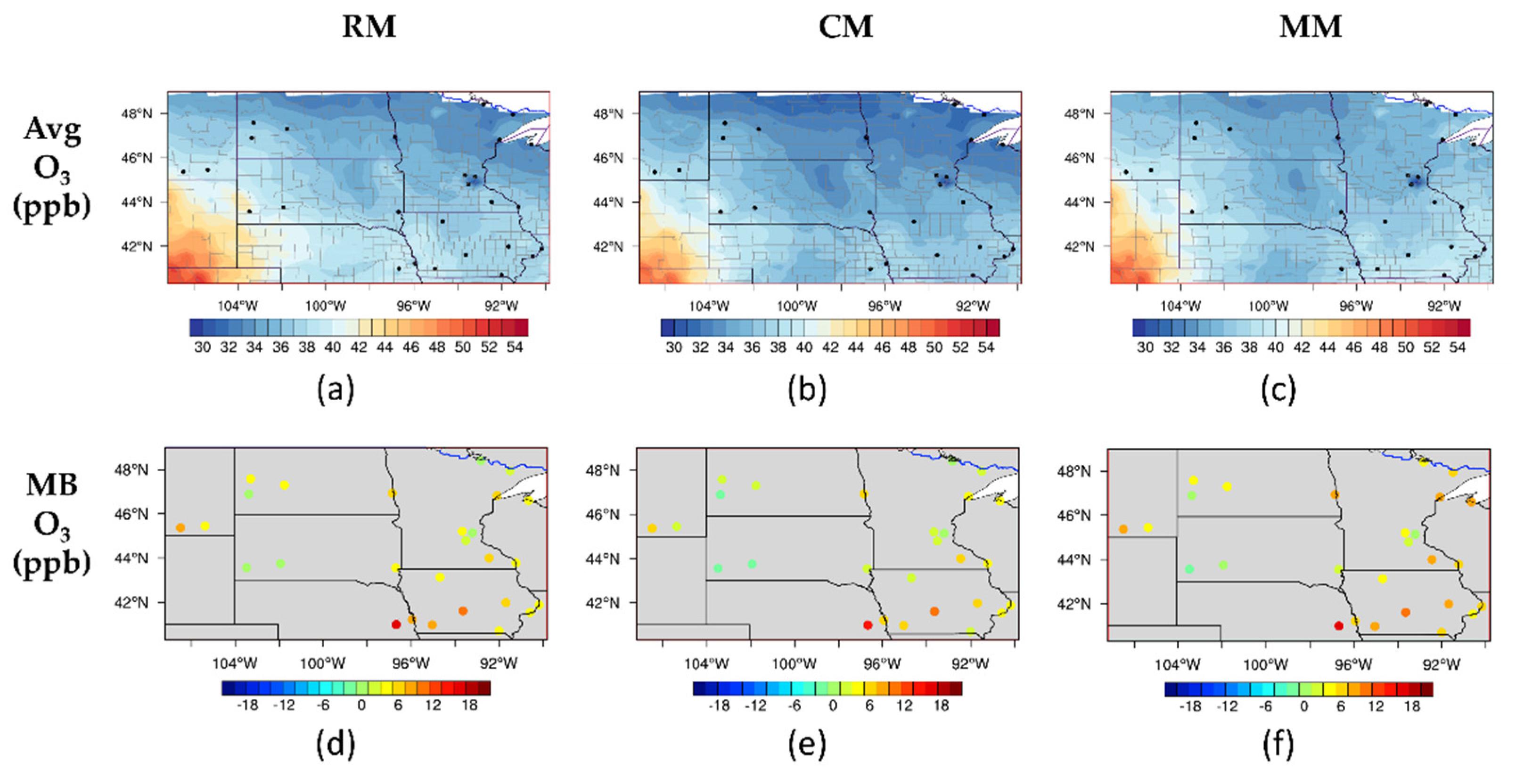
Monthly average O3 predictions are shown in Figure 4a–c. These plots illustrate the similar geographical patterns in the model results of the three chemistry-aerosol mechanisms. Predicted values ranged from the lower 30 ppbs in the north, to the high 30 s in the south, with much higher concentrations in the southwest reaching 50 ppb. Observations values showed a similar pattern of higher concentrations towards the southwest and a slight north-south gradient, but with some variability between individual sites as to be expected with point measurements. Mean bias (MB) results of model predictions compared to observations are presented in Figure 4d–f. Model simulations with all three mechanisms consistently overpredict observations, on average by 4–6 ppb, with larger bias in the east, particularly at southeastern sites, than in the west. This is consistent with a previous study over the conterminous United States which also showed that RACM overpredicted average 24 h ozone concentrations by a similar magnitude [11].
Simulations showed minor differences between mechanisms in average predicted O3 concentration (Figure S1, Supplementary Materials). Averaged across the domain, the MM and RM models produced the highest average O3 concentrations, both with predictions higher than CM by approximately 1.5 ppb. Other comparisons of these gas-phase chemistry mechanisms showed similar or greater differences in average O3 predictions [18,19]. Geographical patterns for the RM and CM mechanism were similar, but with RM consistently higher by around 1 ppb in the east, and 2 ppb on the west of the domain. Results with the MM mechanism, however, showed a somewhat different pattern. Compared with RM, the MM simulations showed concentrations that were higher towards the east by 1–3 ppb, but lower in the southwest by 1–3 ppb. Additionally, compared with CM, MM showed larger positive bias, with concentration differences in the northeast and southeast of up to 4 ppb. The model differences in average O3 share some features with the peak O3 results (Figure S1, Supplementary Materials), but with smaller concentration differences between the models for the monthly averages. In the east, MM tended to predict higher concentrations than the other models, except for the Minneapolis urban area where it predicted less O3, while in the southwest the RM mechanism yielded the highest O3 concentrations. MB and NMB results show the CM mechanism predictions exhibited the least bias at both eastern and western sites, while MM and CM had larger overpredictions, with MM highest at the eastern sites and RM highest at sites in the west.
Model predictions correlated well with observed hourly O3 concentrations. As seen in Table 4, overall Pearson’s correlation coefficients were moderate, with R = 0.52–0.53 for all three mechanisms. Some lack of correlation is expected due to the use of average weekday emissions for all simulation days; for each mechanism, the predictions of eastern sites showed a stronger average correlation coefficient with observations (R = 0.53–0.56) than on western sites (R = 0.45–0.48). The magnitude of average RMSE was also similar for all three mechanisms and for both eastern and western sites, with all values within the range of 10–13 ppb (see Table S6, Supplementary Materials for individual site data).
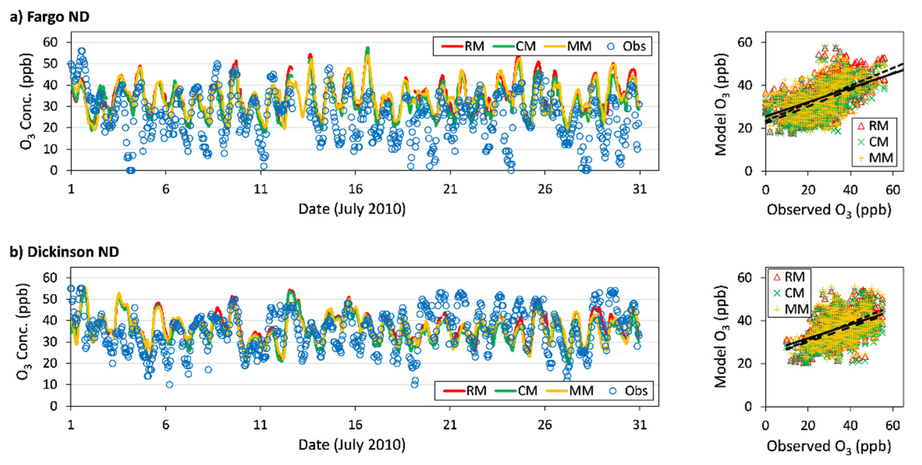
Figure 5 presents hourly O3 concentrations for two sites, Fargo ND and Dickinson ND, representative of eastern and western monitoring sites. Predicted hourly concentrations capture the observed diurnal cycle in ground level O3. However, like many eastern sites, the Fargo results showed a consistent overprediction of results throughout most of the month, generally failing to capture observed nighttime lows below 20 ppb. For the Dickinson site, the models followed observations more closely, while still predicting smaller day/night variations than measured at the site. Scatter plots of both sites also show that model predictions aligned very closely to each other, and evidenced a clear overprediction when observed concentrations were low in all of the models.

3.3. NO2

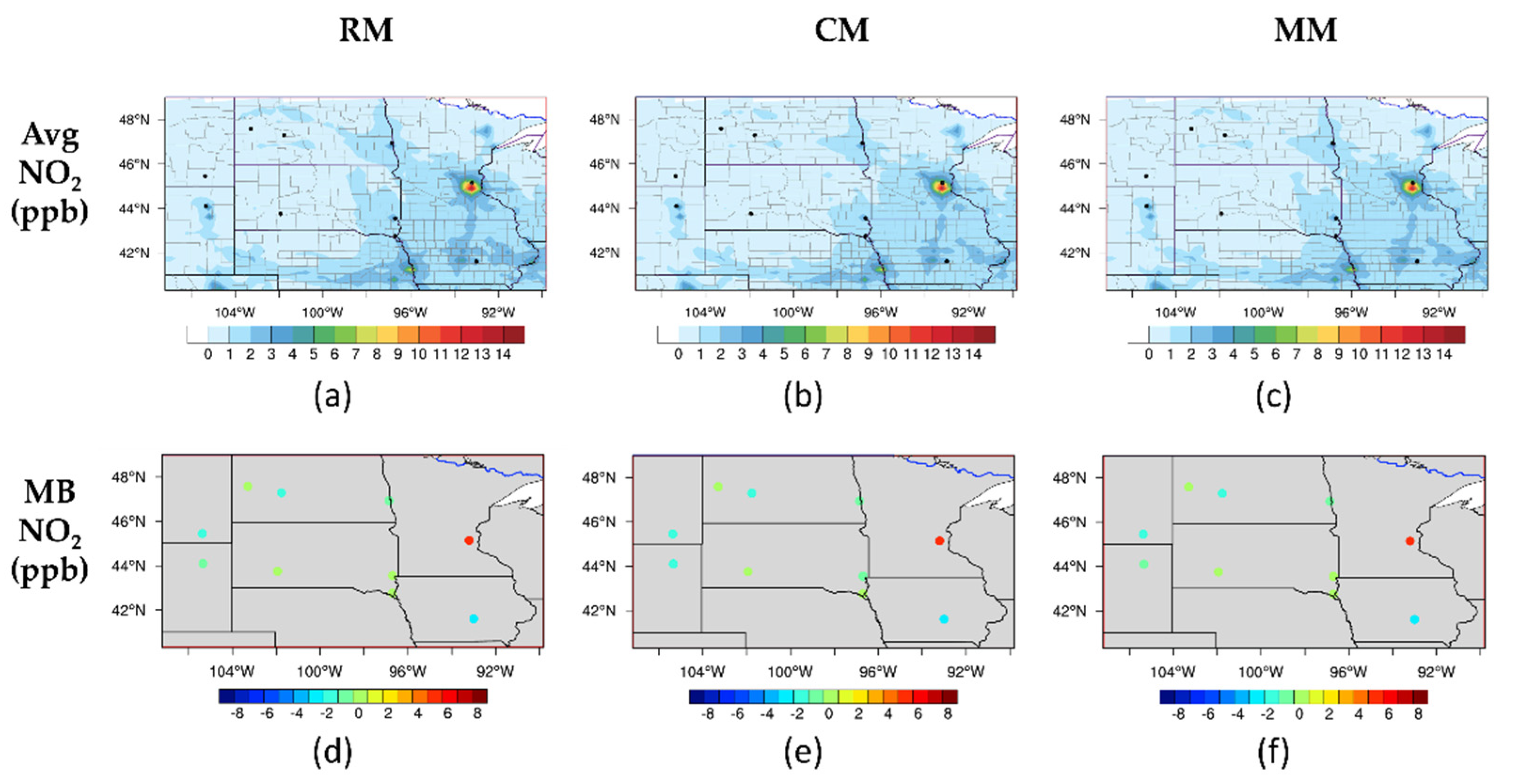
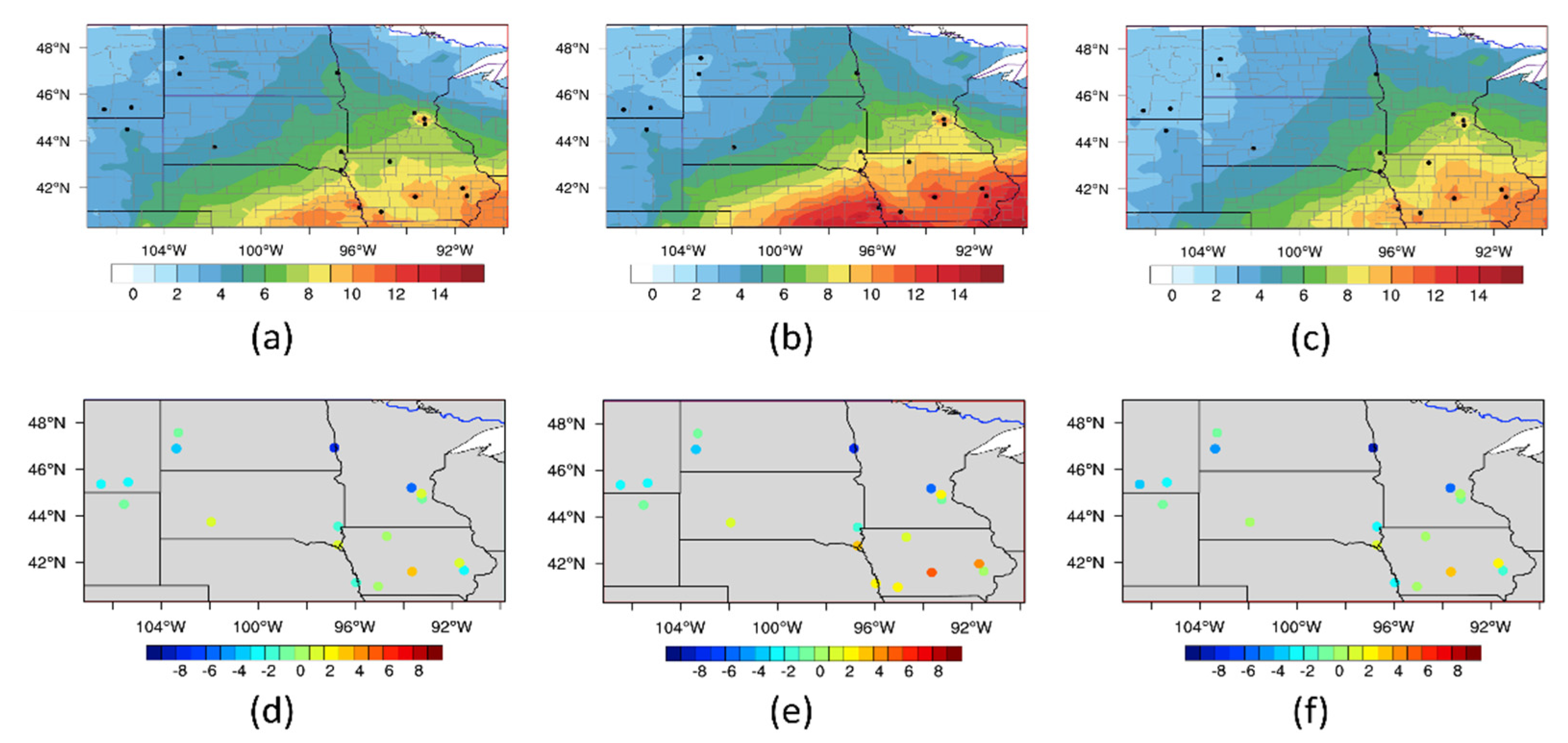
Model predictions of average hourly NO2 concentrations are shown in Figure 6a–c for the RM, CM, and MM chemistry-aerosol mechanisms. The three model predictions appeared very similar to each other, with average NO2 levels less than 1 ppb across much of the western and far northern portions of the domain and slightly higher concentrations of 1–2 ppb in the eastern half of the region. Higher concentrations were predicted at urban centers and along major interstate freeways, with a large peak reaching 14 ppb around Minneapolis, MN. These model predictions generally aligned with the observational data, which reported higher levels in the east, and lower levels in the west, but with elevated levels near Minneapolis MN, Des Moines IA, and Gillette WY. As shown in Figure 6d–f, a slight positive bias of up to 0.5 ppb was observed at many sites, while a negative bias of 1–2 ppb was observed at others. Much larger discrepancies occurred at the monitoring site near Minneapolis, where the models exhibited a high positive bias of 6 ppb, more than doubling the average observed concentration.
Mean NO2 concentration predictions were consistent and extremely similar among the three chemistry mechanisms (Figure S1, Supplementary Materials). The only noticeable differences between models were RM predictions were approximately 0.5 ppb higher at the peak location of the Minneapolis area, and CM showed levels about 0.3 ppb lower in a small area of the southwest, but even those values were within 10% of the other mechanisms. Averaged across the entire domain, RM predictions of NO2 were only slightly higher (0.03 ppb) than MM results, which were slightly higher (0.03 ppb) than CM results. The average relative difference between mechanisms for monthly mean NO2 and O3 were both approximately 5%, but NO2 differences were more uniform across the domain than O3, which had much larger and offsetting geographical variability.
Table 5 provides statistical analysis of the hourly concentration results. Averaged across the 10 NO2 monitoring sites, the predicted monthly average NO2 concentrations for each mechanism were very close to the observed mean of 3.1 ppb, with mean biases smaller than −0.2 ppb. However, these domain average values hide much larger offsetting errors among the individual sites, with underpredictions of 1–2 ppb at several sites, and an overprediction of more than 5 ppb at the site in the Minneapolis area. Comparing model performance at eastern and western sites, MB averaged around −0.8 ppb in the west and about 0.6 ppb in the east, but again with wider variations from site to site. Results for NMB showed a similar pattern, with average overpredictions of 12–19% in the east and underpredictions of 21–28% in the west depending on the model. This range of NMB is consistent with NO2 results reported by other researchers in simulations of the continental U.S. [44,46]. Each of the three models in this study produced similar results. At all locations, the RM mechanism predicted the highest NO2 concentrations, but MM and CM results were always within 10% and 6%, respectively, of the RM values.
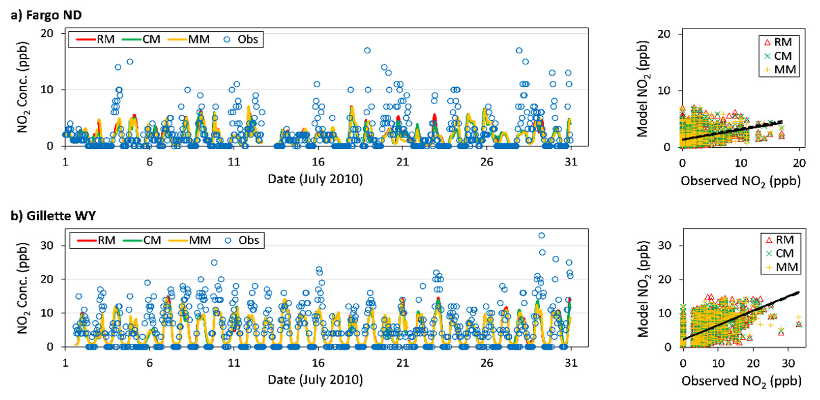
Moderate correlation was seen between model predictions and observed hourly NO2 concentrations for all mechanisms, with domain-wide average R values of 0.38. On average, eastern sites had slightly higher correlation values with R = 0.42 in the east and R = 0.35 in the west, but it is important to remember that these east and west average values are each based on a small number of monitoring sites and that the individual site values ranged more widely, especially in the west (Table S7, Supplementary Materials). The average RMSE (3.2 ppb) was observed to be roughly equal in magnitude to the observed mean concentration (3.1 ppb), and this relationship held true for eastern and western averages as well as for the individual sites. As shown in Figure 7, predicted hourly concentrations of NO2 followed the observed diurnal cycle at both the Fargo ND and Gillette WY sites, while tending to underpredict their nighttime peaks. This is generally true across the other monitoring sites, with the notable exception of the Minneapolis site, where the models significantly overpredicted peak NO2 levels.

3.4. PM2.5

Model predictions of average hourly PM2.5 concentrations are shown in Figure 8a–c for the RM, CM, and MM chemistry-aerosol mechanisms. The three mechanisms appeared to show a similar spatial pattern, with low concentrations in the west and north of less than 5 µg/m3 and higher concentrations in the southeast exceeding 10 µg/m3. Comparing the predictions from each model, some geographical differences are apparent (Figure S1, Supplementary Materials). The CM mechanism showed predictions in the southeast that were up to 4 µg/m3 higher compared with the other mechanisms. The MM mechanism predicted concentrations that were 1–2 µg/m3 higher in the northeast and 0.5 µg/m3 lower in the west compared with the other mechanisms. Predictions for other parts of the domain appeared to be similar in all three mechanisms. Averaged across the entire domain, CM produced the highest PM2.5 concentrations, followed by the RM and MM mechanisms.
The modeled spatial trends in PM2.5 concentrations agreed generally with the observed concentrations. As shown in Table 6, average observed mean values in the east were about twice the western values, 9.8 and 4.8 µg/m3 respectively. Model predictions at the observation sites showed a similar trend with higher concentrations at the eastern monitoring sites on average than at those in the west. However, there were still noticeable differences between modeled and observed concentrations, as seen in Figure 8d–f. In the west, underpredictions of 1–4 µg/m3 occurred at most sites, resulting in an average mean bias of −1.2 to −1.9 µg/m3. In the east, the average bias was smaller, with MB ranging from −1.0 to +0.6 µg/m3. However, this resulted from overpredictions in the southeast, especially with the CM mechanism, which were offset by large underpredictions of 5–8 µg/m3 with all three mechanisms at a pair of sites in the northeast (Table S8, Supplementary Materials).
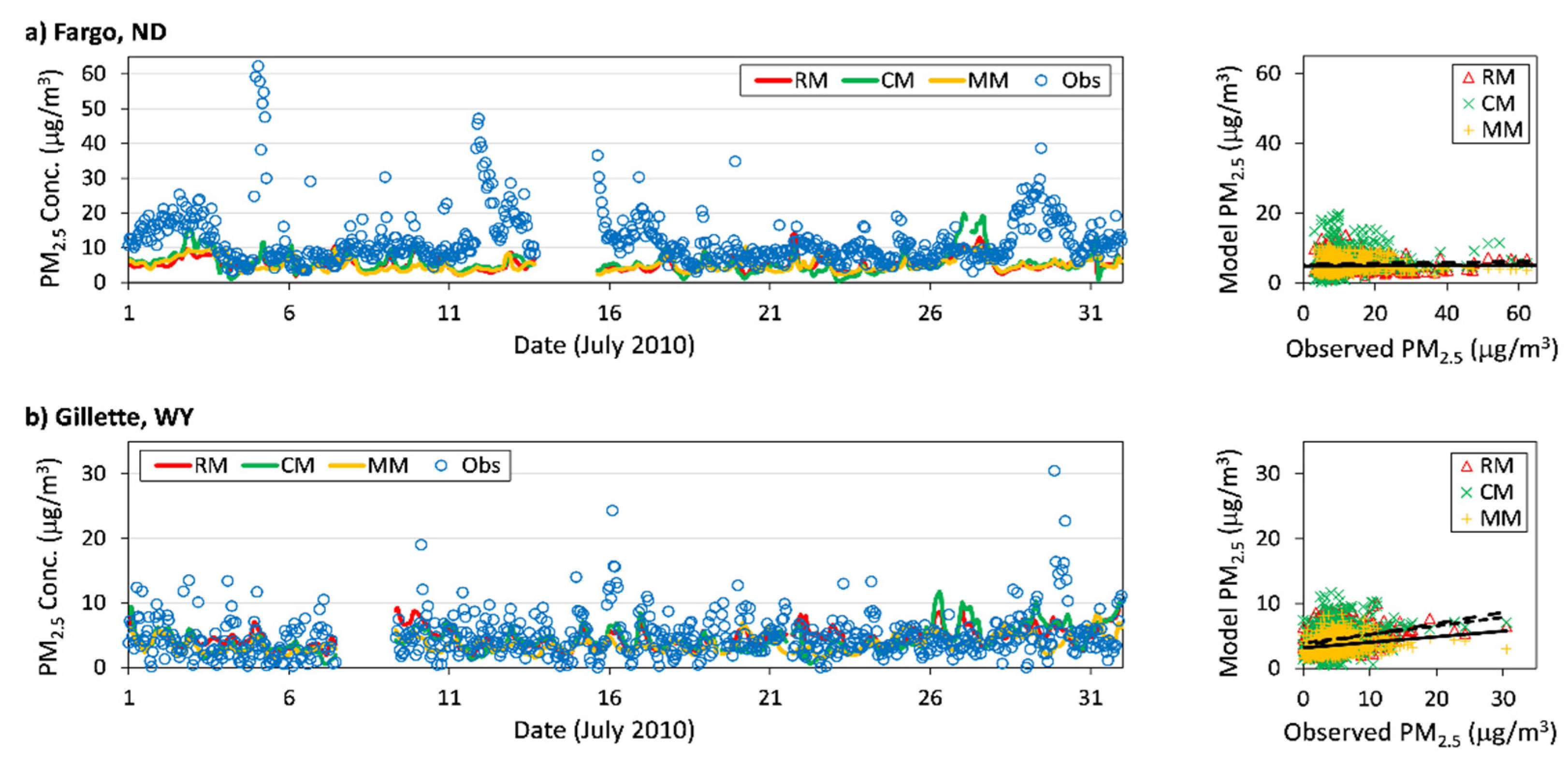
Although the model predictions of average monthly PM2.5 concentrations were fairly close to the observed levels and matched the performance level of other modeling studies [17,46], with NMB values ranging from −14% to +2%, they failed to capture the hourly and daily variability in PM2.5. Pearson’s correlation coefficients were close to zero for all models at most of the sites studied, with average R values ranging from 0.05 to 0.10. Examples of this poor correlation are shown in Figure 9. At the Fargo site, Figure 9a, the models did not predict the observed episodes of elevated PM2.5 levels, nor the hourly variations, resulting in R values of 0.02–0.07. This is in addition to a consistent underprediction for all three mechanisms. Even at the site with the best model-observation agreement, Gillette WY in Figure 9b, the correlation coefficient was only 0.23–0.30. The very poor correlation with hourly PM2.5 data is similar to PM results from previous studies with the same or similar aerosol mechanisms [20,38,41]. Model correlation may be better for daily average, rather than hourly, predictions, as has been seen in other studies [11,17,38,41,72]. However, calculations for a few sites indicated that even for daily average values, while slightly improved, all three models still showed weak correlation with observed PM2.5 concentrations. Considering together the bias and correlation results, there does not appear to be any one mechanism clearly more suitable for predicting PM2.5 concentrations in this region, as all three showed similar errors.

3.5. PM2.5 Subspecies

Before presenting PM2.5 subspecies results, it is important to describe briefly the monitoring sites and measurements that were used. Observational sites for all of the EC, OC, and for some of the SO4 and NO3 subspecies measurements are part of the IMPROVE network of stations which are located in rural areas. Other monitoring sites provide additional measurements of SO4, NO3, and all measurements of NH4. It should be noted that at many of the 25 PM2.5 subspecies sites, observational values for either PM2.5 and/or ozone were not available. Consequently, average results for individual subspecies and for total PM2.5 may not be directly comparable to one another because they are each based on a different set of monitoring sites. Furthermore, the total PM2.5 values include other components that were not individually measured, such as dust and sea salt.
Both of the model aerosol schemes include EC, OC, NO3, NH4, and SO4. These five major aerosol subspecies have corresponding PM2.5 measurement data and were the focus of analysis. Other model aerosol components, such as sodium, chloride, and other inorganics for which measurement data was not available, were not considered individually, but they do contribute to the total simulated PM2.5 mass concentrations. Within the models, the OC fraction is subdivided into multiple subcomponents representing different source or chemical types. Model OC concentrations reported in this work include all of these OC subcomponents, and for the RM and MM models include secondary organic aerosols (SOA). For comparison to observational PM2.5 subspecies data, which are available as daily averages of every third day, model averages of hourly predictions from the corresponding days were used, whereas model-model comparisons used averages of hourly predictions for the entire month.
Model prediction results for PM2.5 subspecies are presented in Figure 10 and Table 7 (See Tables S9–S13 in the Supplementary Materials for individual site results). All three models showed similar geographical patterns for elemental carbon (EC), with areas of higher concentration in the southeast area of the domain, between 0.2 and 0.4 µg/m3, and higher concentration peaks predicted in urban areas. The CBMZ-MOSAIC (CM) chemistry-aerosol mechanism predicted the highest concentrations of EC, with an average simulated EC concentration at the monitoring sites of 0.19 µg/m3, followed by MM (0.18 µg/m3) and RM (0.16 µg/m3). Compared with the average observation value of 0.17 µg/m3, CM and MM slightly overpredicted EC, with NMB values of 20% and 10% respectively, while RM predictions were barely lower than EC observations on average, with a NMB of −2%. Statistical analysis showed a moderate correlation between model predictions and observed concentrations of EC for all mechanisms, with average R values between 0.37 and 0.43. Predicted EC concentrations were similar, but not identical, for the three different mechanisms. EC is a primary pollutant and will depend on emissions, transport, and deposition. Deposition rates and the resulting EC concentrations are influenced by the overall aerosol size distribution and, as noted by other researchers [20], how the size distribution is represented within the model. The RM mechanism uses a modal approach, while CM and MM use a sectional approach to describe the aerosol size distribution. Together with variations in the formation of other aerosol components that affect particle size, this leads to the small differences in predicted EC concentrations shown in Figure 10 and Table 7.
Organic carbon (OC) also showed areas of high concentration towards the southeast of the domain, but these higher levels continue in a band extending northwest. For the RM and CM simulations, OC concentrations were over 0.5 µg/m3 across most of the northeastern third of the domain, with lower concentrations of 0.2–0.3 µg/m3 towards the southwest. The MM simulation, however, showed much higher OC levels, with concentrations over 1 µg/m3 across the eastern third of the domain and exceeding 1.5 µg/m3 in the southeast. The higher OC concentrations with MM are attributable to the SOA components included in this version of the MOSAIC mechanism. While the CM simulation also uses MOSAIC, it does not include any SOA. When considering only primary organic aerosol, the MM predictions were very similar to the CM results. The RM mechanism uses a different SOA scheme that produces much less SOA. All of the models predicted OC concentrations that were lower than observed values. The MM mechanism predicted the highest simulated mean of 0.76 µg/m3, but this was still well below the average observed OC value of 1.18 µg/m3, resulting in NMB of −36%. The RM and CM mechanisms with their even lower OC concentrations had NMB values of −75% and −62%, respectively. Despite these large underpredictions, all three models showed a moderate correlation with the observed OC concentrations, with R values ranging from 0.34 for RM to 0.55 for CM.
Nitrate (NO3) concentrations were highest in the southeast of the domain in all three mechanisms, and were widely dispersed without localized peaks. Maximum predicted concentrations reached 1.8 µg/m3 for the CM mechanism, 1.2 µg/m3 for MM, and 0.8 for RM, with levels dropping below 0.2 µg/m3 across most of the western and northern half of the domain for all three mechanisms. All models significantly overpredicted NO3 concentrations on average. While the observed mean was 0.20 µg/m3, simulated means were 0.57, 0.55, and 0.30 µg/m3 for the CM, MM, and RM mechanisms, respectively. This overestimation is consistent with results from other researchers [17,44,72] who obtained NMB values for NO3 ranging from +30% to +240% with similar models in the U.S. and Europe. The larger NO3 concentrations with CM compared to RM also mirror those reported by Balzarini et al. [17], with the difference attributed to a higher rate constant in CBM-Z for the NO2 + OH → HNO3 reaction. Model-observation correlation was also weak with average R = 0.26–0.28.
Ammonium (NH4) concentrations were more broadly distributed across the domain, with a general north-south gradient for all three mechanisms. Unlike EC, OC, and NO3, where the RM mechanism predicted the lowest concentrations of the three mechanisms, for NH4 it produced the highest concentrations, ranging from 0.2 µg/m3 in the north to over 0.8 µg/m3 in the south. The MM and CM mechanisms produced lower NH4 levels of 0.1–0.2 µg/m3 in the north and 0.3–0.5 µg/m3 in the south. Differences between the mechanism results for NH4 are related to differences in predicted NO3 and SO4 concentrations because aerosol ammonium is primarily formed as H2SO4 and HNO3 are neutralized by NH3 to form (NH4)2SO4 and NH4NO3. As seen in Figure 10, the geographical patterns for NH4 reflect closely a combination of NO3 and SO4 concentrations, with the south-north gradient in NH4 due to SO4 and elevated levels in the southeast due to NO3. At the 6 NH4 monitoring sites, which were mainly in the southeast, the RM mechanism produced a simulated mean of 0.75 µg/m3, compared with the observed average value of 0.49 µg/m3. The MM and CM mechanisms also overpredicted mean NH4 concentration, but to a lesser extent. Average NMB was 65% for RM, and only 25% and 11% for MM and CM, respectively. Statistical analysis, however, showed essentially no correlation between model and observed NH4 concentrations for any of the mechanisms, as the average Pearson’s correlation coefficient was between −0.01 and 0.06.
Sulfate (SO4) showed an increasing trend towards the south and southwest of the domain in all three mechanisms, with no localized peaks predicted. The CM mechanism predicted the lowest SO4 levels with average concentrations ranging from approximately 0.5 µg/m3 across most of the domain to 1.0 µg/m3 in the far southeast corner. The MM mechanism had a similar north south trend, but was uniformly higher across the entire domain by about 0.75 µg/m3. The RM mechanism predicted the largest north-south gradient, ranging from less than 0.5 µg/m3 in the north to almost 2 µg/m3 in the south. In comparisons of model predictions with monitoring site data, the RM mechanism produced the highest simulated mean of 1.26 µg/m3, followed by the MM prediction of 1.20 µg/m3. Both predictions were slightly higher than the observed average value of 1.18 µg/m3, resulting in NMB values of approximately 30%. The CM mechanism predictions were much lower at only 0.53 µg/m3 and NMB of −37%. This is likely due to an underprediction of aqueous SO2 oxidation to form SO4 as has been suggested by other researchers [17,73]. Consistent with this explanation, in the present study SO2 concentrations with CM were higher than with RM and MM. Similar behavior has been seen in other studies where simulations using CM significantly underestimate observed sulfate concentrations [73], and predict much less sulfate than simulations using MM and RM [17,20]. Statistical analysis showed near null Pearson’s correlation coefficients for all three mechanisms, with R between −0.15 and +0.13.
Variability in model performance for the different aerosol subspecies depends on how well the gas and aerosol mechanisms capture the underlying formation processes, especially for secondary species. All three mechanisms performed relatively well on EC predictions, with average NMB less than 20% and moderate correlation to hourly observations. As a primary pollutant, modeled EC concentrations depend on emissions inventories, which were the same in all simulations, as well as on transport, dispersion, and removal processes, which were similar across the three models. Consequently, it is not surprising the model results were similar to each other. The good agreement with observations suggests the emission inventories for EC are reasonably accurate. Organic carbon predictions also showed moderate correlation with observations, but unlike EC, OC was significantly underpredicted. For RM and CM mechanisms, the average NMB was more than −60%, and while MM predicted higher concentrations, especially in the eastern portion of the domain, it also underpredicted observations, with an average NMB of −36%. These prediction errors are likely due to uncertainties in representation of SOA process and precursors in the gas-aerosol mechanisms, as well as uncertainties in POA and SOA emissions [74]. The RM simulation uses a limited SOA representation with the SORGAM scheme, but still produced lower OC concentrations than CM, which did not account for any SOA. The MM simulation uses the same MOSAIC aerosol scheme as CM, but with SOA, and this appeared to lead to better predictions. However, even with the inclusion of some SOA processes, RM and MM simulations still produced poor overall OC prediction results, suggesting that errors in organic aerosol representation remain.
For the secondary inorganic aerosol species (NO3, NH4, and SO4), predictions from all of the models showed a very poor correlation with the hourly measurements from monitoring sites. Monthly averages also had significant errors that varied depending on the model and aerosol species, further highlighting uncertainties in simulating aerosol processes as has been noted by other researchers [11,17,20,72,74,75]. Results of this study show that RM overpredicted NH4, but performed reasonably well with both NO3 and SO4. The CM mechanism, on the other hand, had minimal error with NH4, but overpredicted NO3 and underpredicted SO4, both by more than a factor of 2. MM had similar overpredictions of NO3 as CM, but performed much better with NH4 and SO4. Comparing these results to previous WRF-Chem simulations is difficult, as other studies do not show consistent trends for NO3 and SO4 predictions between different mechanisms. For example, our results are similar to WRF-Chem studies by Balzarini and coworkers [17] and Zhang and coworkers [44], who found NO3 was overestimated by CM, RADM2-MADE/SORGAM, and other mechanisms. However, results from Georgiou [20] and Tessum [11] found that CM, MM, and RACM-MADE/VBS all underpredicted nitrate concentrations. Additionally, while Balzarini [17] and Georgiou [20] showed CM underpredicting SO4, similar to our work, they attribute this negative bias to the absence of aqueous phase SO2 oxidation reactions. That explanation does not fit with the results from this work, where the CM and RM simulations did include aqueous reactions, and MM did not, but it was only the CM results that underpredicted SO4. In better agreement are particulate ammonium predictions, where NH4 concentrations follow SO4 and NO3, due to the formation of (NH4)2SO4 and NH4NO3, and were consistently overpredicted by all three mechanisms in this study and matched or exceeded observations in other reported studies [11,17,20,44].

4. Conclusions

The WRF-Chem online coupled atmospheric chemistry model was used to simulate gas and aerosol concentrations over the Northern Great Plains for July 2010, prior to the significant increase in oil production activities over the following years. The performance of the CBMZ-MOSAIC (CM), RACM-MADE/SORGAM (RMS), and MOZART-MOSAIC (MM) gas-chemistry aerosol mechanisms were analyzed against each other and against ground level observations. All three gas-aerosol mechanism combinations produced generally similar results for both monthly averages and diurnal variations in hourly concentrations. Ozone and NO2 predictions were within 5% of each other on average, while average PM2.5 concentrations varied between mechanisms by less than 20%. Aerosol subspecies results showed much greater variability between mechanisms (differences of more than a factor of two in some cases) with RM predicting less nitrate, CM less sulfate and ammonium, and MM more organic carbon.
When evaluated against observational data, all simulations were able to reproduce hourly meteorological measurements for temperature, pressure, and relative humidity with good correlation, minimal bias, and little geographical variation in performance. Wind speed prediction performance showed moderate correlation to observations, with overpredictions at western sites and underpredictions at eastern sites. Performance for O3 and NO2 was reasonable, with all mechanisms showing moderate correlation to hourly measurements and average NMB of approximately +20% for O3 and −5% for NO2, but with NO2 overpredicted in the east and underpredicted in the west. Model performance was not as good for fine particulate. Monthly average PM2.5 concentrations were relatively accurate, but with very low correlation to hourly measurements. Aerosol subspecies predictions showed low correlation and, with the exception of EC, significant bias, underpredicting OC, overpredicting NO3 and NH4, and over or underpredicting SO4 depending on the mechanism.
Measured and modeled pollutant concentrations for this time period are relatively low across the mostly rural study domain. O3, NO2, and PM2.5 levels are all well below NAAQS standards. Some geographical variations exist in pollutant levels. Monthly average O3 is highest in the southwest of the domain and lowest in the north. Model simulations show the highest NO2 concentrations around the Minneapolis-St. Paul metropolitan area, higher levels in the south and east along major transportation and population centers, and the lowest concentrations in the northwest. PM2.5 concentrations show a strong gradient from highest levels in the south and southeast to lowest in the north and northwest. Predicted fine aerosol subspecies concentrations also show strong geographical patterns. EC and NO3 behave similarly to NO2, with higher levels in the south and southeast and lower levels in the northwest. NH4 and SO4 concentrations are highest in the south and lowest in the north. OC has a gradient from high levels in the east to lower in the west.
For future model simulations of this region, any of the mechanisms appear suitable for predicting gas phase concentrations and particle phase predictions show similar levels of uncertainty. The July 2010 scenario in this study was specifically chosen to capture baseline conditions for the Bakken region before increased oil and gas production activities would have influenced air quality. Modeling results for this time period indicate that, in general, the northwestern portion of the study domain, where the Bakken oil and gas fields are located, had the lowest pollutant concentrations. Additional studies of the region that include the more recent increases in oil and gas-related emissions can use these results as a basis of comparison.

Supplementary Materials

The following are available online at https://www.mdpi.com/article/10.3390/atmos12091121/s1, Figure S1: Differences between model predictions of maximum hourly O3, mean O3, NO2, and PM2.5 concentrations, Table S1: Meteorology and air quality monitoring sites and available measurements, Table S2: Statistical analysis of predicted hourly near ground temperature at individual monitoring sites, Table S3: Statistical analysis of predicted hourly surface pressure at individual monitoring sites, Table S4: Statistical analysis of predicted hourly relative humidity at individual monitoring sites, Table S5: Statistical analysis of predicted hourly 10 m wind speed at individual monitoring sites, Table S6: Statistical analysis of predicted hourly O3 concentrations at individual monitoring sites, Table S7: Statistical analysis of predicted hourly NO2 concentrations at individual monitoring sites, Table S8: Statistical analysis of predicted hourly PM2.5 concentrations at individual monitoring sites, Table S9: Statistical analysis of predicted daily average PM2.5 elemental carbon (EC) concentrations, Table S10: Statistical analysis of predicted daily average PM2.5 organic carbon (OC) concentrations, Table S11: Statistical analysis of predicted daily average PM2.5 nitrate (NO3) concentrations, Table S12: Statistical analysis of predicted daily average PM2.5 ammonium (NH4) concentrations, Table S13: Statistical analysis of predicted daily average PM2.5 sulfate (SO4) concentrations.

Author Contributions

Conceptualization, F.M.B. and C.J.B.; methodology, C.J.B.; software, C.J.B.; validation, C.J.B. and F.M.B.; formal analysis, C.J.B.; investigation, C.J.B.; resources, F.M.B.; data curation, C.J.B. and F.M.B.; writing—original draft preparation, C.J.B. and F.M.B.; writing—review and editing, F.M.B. and C.J.B.; visualization, C.J.B. and F.M.B.; supervision, F.M.B.; project administration, F.M.B.; funding acquisition, F.M.B. All authors have read and agreed to the published version of the manuscript.

Funding

This material is based upon work supported by the National Science Foundation under Grant No. OIA-1355466.

Institutional Review Board Statement

Not applicable.

Informed Consent Statement

Not applicable.

Data Availability Statement

The data presented in this study are available in the Supplementary Materials. Additional data are available on request from the corresponding author.

Acknowledgments

The authors would like to acknowledge Stuart McKeen from the National Oceanic and Atmospheric Administration for providing the National Emission Inventory 2011 (NEI-2011) data suitable for WRF-Chem digestion. We acknowledge use of the WRF-Chem preprocessor tool {mozbc, EPA_ANTHRO_EMISS, and bio_emiss} provided by the Atmospheric Chemistry Observations and Modeling Lab (ACOM) of NCAR. In addition, we also acknowledge Shawn Jaker for providing codes for the extraction of WRF-Chem model outputs, Aaron Scott for reviewing the initial meteorological data, Adam Lawman for Linux support, and Aaron Bergstrom for support using the UND Computational Research Center.

Conflicts of Interest

The authors declare no conflict of interest. The funders had no role in the design of the study; in the collection, analyses, or interpretation of data; in the writing of the manuscript, or in the decision to publish the results.

References

  1. Allen, D.T. Emissions from oil and gas operations in the United States and their air quality implications. J. Air Waste Manag. Assoc. 2016, 66, 549–575. [Google Scholar] [CrossRef] [Green Version]
  2. Evanoski-Cole, A.R.; Gebhart, K.A.; Sive, B.C.; Zhou, Y.; Capps, S.L.; Day, D.E.; Prenni, A.J.; Schurman, M.I.; Sullivan, A.P.; Li, Y.; et al. Composition and sources of winter haze in the Bakken oil and gas extraction region. Atmos. Environ. 2017, 156, 77–87. [Google Scholar] [CrossRef]
  3. Homepage—U.S. Energy Information Administration (EIA). Available online: https://www.eia.gov/index.php (accessed on 2 July 2021).
  4. Li, C.; Hsu, N.C.; Sayer, A.M.; Krotkov, N.A.; Fu, J.S.; Lamsal, L.N.; Lee, J.; Tsay, S.-C. Satellite observation of pollutant emissions from gas flaring activities near the Arctic. Atmos. Environ. 2016, 133, 1–11. [Google Scholar] [CrossRef]
  5. Majid, A.; Martin, M.V.; Lamsal, L.N.; Duncan, B.N. A decade of changes in nitrogen oxides over regions of oil and natural gas activity in the United States. Elementa-Sci. Anthrop. 2017, 5, 76. [Google Scholar] [CrossRef]
  6. Prenni, A.J.; Day, D.E.; Evanoski-Cole, A.R.; Sive, B.C.; Hecobian, A.; Zhou, Y.; Gebhart, K.A.; Hand, J.L.; Sullivan, A.P.; Li, Y.; et al. Oil and gas impacts on air quality in federal lands in the Bakken region: An overview of the Bakken Air Quality Study and first results. Atmos. Chem. Phys. 2016, 16, 1401–1416. [Google Scholar] [CrossRef] [Green Version]
  7. Schwarz, J.P.; Holloway, J.S.; Katich, J.M.; McKeen, S.; Kort, E.A.; Smith, M.L.; Ryerson, T.B.; Sweeney, C.; Peischl, J. Black Carbon Emissions from the Bakken Oil and Gas Development Region. Environ. Sci. Technol. Lett. 2015, 2, 281–285. [Google Scholar] [CrossRef]
  8. Thompson, T.M.; Shepherd, D.; Stacy, A.; Barna, M.G.; Schichtel, B.A. Modeling to Evaluate Contribution of Oil and Gas Emissions to Air Pollution. J. Air Waste Manag. Assoc. 2017, 67, 445–461. [Google Scholar] [CrossRef] [PubMed] [Green Version]
  9. Nopmongcol, U.; Alvarez, Y.; Jung, J.; Grant, J.; Kumar, N.; Yarwood, G. Source contributions to United States ozone and particulate matter over five decades from 1970 to 2020. Atmos. Environ. 2017, 167, 116–128. [Google Scholar] [CrossRef]
  10. Yahya, K.; Wang, K.; Campbell, P.; Chen, Y.; Glotfelty, T.; He, J.; Pirhalla, M.; Zhang, Y. Decadal application of WRF/Chem for regional air quality and climate modeling over the US under the representative concentration pathways scenarios. Part 1: Model evaluation and impact of downscaling. Atmos. Environ. 2017, 152, 562–583. [Google Scholar] [CrossRef] [Green Version]
  11. Tessum, C.W.; Hill, J.D.; Marshall, J.D. Twelve-month, 12 km resolution North American WRF-Chem v3.4 air quality simulation: Performance evaluation. Geosci. Model. Dev. 2015, 8, 957–973. [Google Scholar] [CrossRef] [Green Version]
  12. Yahya, K.; Campbell, P.; Zhang, Y. Decadal application of WRF/chem for regional air quality and climate modeling over the US under the representative concentration pathways scenarios. Part 2: Current vs. future simulations. Atmos. Environ. 2017, 152, 584–604. [Google Scholar] [CrossRef] [Green Version]
  13. Abdallah, C.; Sartelet, K.; Afif, C. Influence of boundary conditions and anthropogenic emission inventories on simulated O3 and PM2.5 concentrations over Lebanon. Atmos. Pollut. Res. 2016, 7, 971–979. [Google Scholar] [CrossRef] [Green Version]
  14. Werner, M.; Kryza, M.; Geels, C.; Ellermann, T.; Ambelas Skjøth, C. Ammonia Concentrations Over Europe—Application of the WRF-Chem Model Supported with Dynamic Emission. Pol. J. Environ. Stud. 2017, 26, 1323–1341. [Google Scholar] [CrossRef]
  15. Im, U.; Christensen, J.H.; Geels, C.; Hansen, K.M.; Brandt, J.; Solazzo, E.; Alyuz, U.; Balzarini, A.; Baro, R.; Bellasio, R.; et al. Influence of anthropogenic emissions and boundary conditions on multi-model simulations of major air pollutants over Europe and North America in the framework of AQMEII3. Atmos. Chem. Phys. 2018, 18, 8929–8952. [Google Scholar] [CrossRef] [PubMed] [Green Version]
  16. Gupta, M.; Mohan, M. Validation of WRF/Chem model and sensitivity of chemical mechanisms to ozone simulation over megacity Delhi. Atmos. Environ. 2015, 122, 220–229. [Google Scholar] [CrossRef]
  17. Balzarini, A.; Pirovano, G.; Honzak, L.; Zabkar, R.; Curci, G.; Forkel, R.; Hirtl, M.; San Jose, R.; Tuccella, P.; Grell, G.A. WRF-Chem model sensitivity to chemical mechanisms choice in reconstructing aerosol optical properties. Atmos. Environ. 2015, 115, 604–619. [Google Scholar] [CrossRef]
  18. Im, U.; Bianconi, R.; Solazzo, E.; Kioutsioukis, I.; Badia, A.; Balzarini, A.; Baro, R.; Bellasio, R.; Brunner, D.; Chemel, C.; et al. Evaluation of operational on-line-coupled regional air quality models over Europe and North America in the context of AQMEII phase 2. Part I: Ozone. Atmos. Environ. 2015, 115, 404–420. [Google Scholar] [CrossRef] [Green Version]
  19. Mar, K.A.; Ojha, N.; Pozzer, A.; Butler, T.M. Ozone air quality simulations with WRF-Chem (v3.5.1) over Europe: Model evaluation and chemical mechanism comparison. Geosci. Model. Dev. 2016, 9, 3699–3728. [Google Scholar] [CrossRef] [Green Version]
  20. Georgiou, G.K.; Christoudias, T.; Proestos, Y.; Kushta, J.; Hadjinicolaou, P.; Lelieveld, J. Air quality modelling in the summer over the eastern Mediterranean using WRF-Chem: Chemistry and aerosol mechanism intercomparison. Atmos. Chem. Phys. 2018, 18, 1555–1571. [Google Scholar] [CrossRef] [Green Version]
  21. Appel, K.W.; Napelenok, S.L.; Foley, K.M.; Pye, H.O.T.; Hogrefe, C.; Luecken, D.J.; Bash, J.O.; Roselle, S.J.; Pleim, J.E.; Foroutan, H.; et al. Description and evaluation of the Community Multiscale Air Quality (CMAQ) modeling system version 5.1. Geosci. Model. Dev. 2017, 10, 1703–1732. [Google Scholar] [CrossRef] [Green Version]
  22. Grell, G.A.; Peckham, S.E.; Schmitz, R.; McKeen, S.A.; Frost, G.; Skamarock, W.C.; Eder, B. Fully coupled “online” chemistry within the WRF model. Atmos. Environ. 2005, 39, 6957–6975. [Google Scholar] [CrossRef]
  23. Ramboll Environment and Health. User’s Guide Comprehensive Air Quality Model with Extensions Version 7.10; CAMx: Anaheim, CA, USA, 2020. [Google Scholar]
  24. Long, M.S.; Yantosca, R.; Nielsen, J.E.; Keller, C.A.; da Silva, A.; Sulprizio, M.P.; Pawson, S.; Jacob, D.J. Development of a grid-independent GEOS-Chem chemical transport model (v9-02) as an atmospheric chemistry module for Earth system models. Geosci. Model. Dev. 2015, 8, 595–602. [Google Scholar] [CrossRef] [Green Version]
  25. Mailler, S.; Menut, L.; Khvorostyanov, D.; Valari, M.; Couvidat, F.; Siour, G.; Turquety, S.; Briant, R.; Tuccella, P.; Bessagnet, B.; et al. CHIMERE-2017: From urban to hemispheric chemistry-transport modeling. Geosci. Model. Dev. 2017, 10, 2397–2423. [Google Scholar] [CrossRef] [Green Version]
  26. Zaveri, R.A.; Peters, L.K. A new lumped structure photochemical mechanism for large-scale applications. J. Geophys. Res. Atmos. 1999, 104, 30387–30415. [Google Scholar] [CrossRef]
  27. Gery, M.W.; Whitten, G.Z.; Killus, J.P.; Dodge, M.C. A photochemical kinetics mechanism for urban and regional scale computer modeling. J. Geophys. Res. Atmos. 1989, 94, 12925–12956. [Google Scholar] [CrossRef]
  28. Stockwell, W.R.; Middleton, P.; Chang, J.S.; Tang, X. The second generation regional acid deposition model chemical mechanism for regional air quality modeling. J. Geophys. Res. Atmos. 1990, 95, 16343–16367. [Google Scholar] [CrossRef]
  29. Stockwell, W.R.; Kirchner, F.; Kuhn, M.; Seefeld, S. A new mechanism for regional atmospheric chemistry modeling. J. Geophys. Res. Atmos. 1997, 102, 25847–25879. [Google Scholar] [CrossRef] [Green Version]
  30. Carter, W.P.L. Documentation of the SAPRC-99 Chemical Mechanism for VOC Reactivity Assessment; California Air Resources Board, Research Division: Sacramento, CA, USA, 2000. [Google Scholar]
  31. Emmons, L.K.; Walters, S.; Hess, P.G.; Lamarque, J.-F.; Pfister, G.G.; Fillmore, D.; Granier, C.; Guenther, A.; Kinnison, D.; Laepple, T.; et al. Description and evaluation of the Model for Ozone and Related chemical Tracers, version 4 (MOZART-4). Geosci. Model. Dev. 2010, 3, 43–67. [Google Scholar] [CrossRef] [Green Version]
  32. Zaveri, R.A.; Easter, R.C.; Fast, J.D.; Peters, L.K. Model for Simulating Aerosol Interactions and Chemistry (MOSAIC). J. Geophys. Res. Atmos. 2008, 113, D13204. [Google Scholar] [CrossRef]
  33. Ackermann, I.J.; Hass, H.; Memmesheimer, M.; Ebel, A.; Binkowski, F.S.; Shankar, U. Modal aerosol dynamics model for Europe: Development and first applications. Atmos. Environ. 1998, 32, 2981–2999. [Google Scholar] [CrossRef]
  34. Schell, B.; Ackermann, I.J.; Hass, H.; Binkowski, F.S.; Ebel, A. Modeling the formation of secondary organic aerosol within a comprehensive air quality model system. J. Geophys. Res. Atmos. 2001, 106, 28275–28293. [Google Scholar] [CrossRef]
  35. Ahmadov, R.; McKeen, S.A.; Robinson, A.L.; Bahreini, R.; Middlebrook, A.M.; de Gouw, J.A.; Meagher, J.; Hsie, E.-Y.; Edgerton, E.; Shaw, S.; et al. A volatility basis set model for summertime secondary organic aerosols over the eastern United States in 2006. J. Geophys. Res. Atmos. 2012, 117, D06301. [Google Scholar] [CrossRef]
  36. Sartelet, K.N.; Hayami, H.; Albriet, B.; Sportisse, B. Development and preliminary validation of a modal aerosol model for tropospheric chemistry: MAM. Aerosol Sci. Technol. 2006, 40, 118–127. [Google Scholar] [CrossRef]
  37. Chin, M.; Rood, R.B.; Lin, S.J.; Muller, J.F.; Thompson, A.M. Atmospheric sulfur cycle simulated in the global model GOCART: Model description and global properties. J. Geophys. Res. Atmos. 2000, 105, 24671–24687. [Google Scholar] [CrossRef]
  38. Do, T.N.N.; Ngo, X.T.; Pham, V.H.; Vuong, N.L.; Le, H.A.; Pham, C.T.; Bui, Q.H.; Nguyen, T.N.T. Application of WRF-Chem to simulate air quality over Northern Vietnam. Environ. Sci. Pollut. Res. 2021, 28, 12067–12081. [Google Scholar] [CrossRef] [PubMed]
  39. Kushta, J.; Georgiou, G.K.; Proestos, Y.; Christoudias, T.; Lelieveld, J. Modelling study of the atmospheric composition over Cyprus. Atmos. Pollut. Res. 2018, 9, 257–269. [Google Scholar] [CrossRef]
  40. Spiridonov, V.; Jakimovski, B.; Spiridonova, I.; Pereira, G. Development of air quality forecasting system in Macedonia, based on WRF-Chem model. Air Qual. Atmos. Health 2019, 12, 825–836. [Google Scholar] [CrossRef] [Green Version]
  41. Ritter, M.; Mueller, M.D.; Tsai, M.-Y.; Parlow, E. Air pollution modeling over very complex terrain: An evaluation of WRF-Chem over Switzerland for two 1-year periods. Atmos. Res. 2013, 132, 209–222. [Google Scholar] [CrossRef]
  42. Tie, X.; Brasseur, G.; Ying, Z. Impact of model resolution on chemical ozone formation in Mexico City: Application of the WRF-Chem model. Atmos. Chem. Phys. 2010, 10, 8983–8995. [Google Scholar] [CrossRef] [Green Version]
  43. Wang, P.; Qiao, X.; Zhang, H. Modeling PM2.5 and O-3 with aerosol feedbacks using WRF/Chem over the Sichuan Basin, southwestern China. Chemosphere 2020, 254, 126735. [Google Scholar] [CrossRef]
  44. Zhang, Y.; Chen, Y.; Sarwar, G.; Schere, K. Impact of gas-phase mechanisms on Weather Research Forecasting Model with Chemistry (WRF/Chem) predictions: Mechanism implementation and comparative evaluation. J. Geophys. Res. Atmos. 2012, 117, D01301. [Google Scholar] [CrossRef] [Green Version]
  45. Knote, C.; Tuccella, P.; Curci, G.; Emmons, L.; Orlando, J.J.; Madronich, S.; Baro, R.; Jimenez-Guerrero, P.; Luecken, D.; Hogrefe, C.; et al. Influence of the choice of gas-phase mechanism on predictions of key gaseous pollutants during the AQMEII phase-2 intercomparison. Atmos. Environ. 2015, 115, 553–568. [Google Scholar] [CrossRef]
  46. Yahya, K.; Wang, K.; Gudoshava, M.L.; Glotfelty, T.; Zhang, Y. Application of WRF/Chem over North America under the AQMEII Phase 2: Part I. Comprehensive evaluation of 2006 simulation. Atmos. Environ. 2015, 115, 733–755. [Google Scholar] [CrossRef]
  47. Derwent, R. Intercomparison of chemical mechanisms for air quality policy formulation and assessment under North American conditions. J. Air Waste Manag. Assoc. 2017, 67, 789–796. [Google Scholar] [CrossRef] [PubMed] [Green Version]
  48. Mallula, S. Effects Of Non-Conventional Gas And Oil Production Activities On Local And Regional Fine Particles And Ground-Level Ozone. Ph.D. Thesis, University of North Dakota, Grand Forks, ND, USA, 2017. [Google Scholar]
  49. Fast, J.D.; Gustafson, W.I.; Easter, R.C.; Zaveri, R.A.; Barnard, J.C.; Chapman, E.G.; Grell, G.A.; Peckham, S.E. Evolution of ozone, particulates, and aerosol direct radiative forcing in the vicinity of Houston using a fully coupled meteorology-chemistry-aerosol model. J. Geophys. Res. Atmos. 2006, 111, D21305. [Google Scholar] [CrossRef]
  50. Damian, V.; Sandu, A.; Damian, M.; Potra, F.; Carmichael, G.R. The kinetic preprocessor KPP—A software environment for solving chemical kinetics. Comput. Chem. Eng. 2002, 26, 1567–1579. [Google Scholar] [CrossRef]
  51. Sandu, A.; Sander, R. Technical note: Simulating chemical systems in Fortran90 and Matlab with the Kinetic PreProcessor KPP-2.1. Atmos. Chem. Phys. 2006, 6, 187–195. [Google Scholar] [CrossRef] [Green Version]
  52. Morrison, H.; Thompson, G.; Tatarskii, V. Impact of Cloud Microphysics on the Development of Trailing Stratiform Precipitation in a Simulated Squall Line: Comparison of One- and Two-Moment Schemes. Mon. Weather Rev. 2009, 137, 991–1007. [Google Scholar] [CrossRef] [Green Version]
  53. Iacono, M.J.; Delamere, J.S.; Mlawer, E.J.; Shephard, M.W.; Clough, S.A.; Collins, W.D. Radiative forcing by long-lived greenhouse gases: Calculations with the AER radiative transfer models. J. Geophys. Res. Atmos. 2008, 113, D13103. [Google Scholar] [CrossRef]
  54. Chen, F.; Dudhia, J. Coupling an advanced land surface-hydrology model with the Penn State-NCAR MM5 modeling system. Part I: Model implementation and sensitivity. Mon. Weather Rev. 2001, 129, 569–585. [Google Scholar] [CrossRef] [Green Version]
  55. Hong, S.-Y.; Noh, Y.; Dudhia, J. A new vertical diffusion package with an explicit treatment of entrainment processes. Mon. Weather Rev. 2006, 134, 2318–2341. [Google Scholar] [CrossRef] [Green Version]
  56. Grell, G.A.; Devenyi, D. A generalized approach to parameterizing convection combining ensemble and data assimilation techniques. Geophys. Res. Lett. 2002, 29, 1693. [Google Scholar] [CrossRef] [Green Version]
  57. Wild, O.; Zhu, X.; Prather, M.J. Fast-j: Accurate simulation of in- and below-cloud photolysis in tropospheric chemical models. J. Atmos. Chem. 2000, 37, 245–282. [Google Scholar] [CrossRef]
  58. US EPA, OAR Air Quality System (AQS). Available online: https://www.epa.gov/aqs (accessed on 2 July 2021).
  59. North Dakota Drilling and Production Statistics. Available online: https://www.dmr.nd.gov/oilgas/stats/statisticsvw.asp (accessed on 2 July 2021).
  60. Mesinger, F.; DiMego, G.; Kalnay, E.; Mitchell, K.; Shafran, P.C.; Ebisuzaki, W.; Jovic, D.; Woollen, J.; Rogers, E.; Berbery, E.H.; et al. North American regional reanalysis. Bull. Am. Meteorol. Soc. 2006, 87, 343–360. [Google Scholar] [CrossRef] [Green Version]
  61. US Environmental Protection Agency, Office of Air Quality Planning and Standards. Technical Support Document (TSD) Preparation of Emissions Inventories for the Version 6.3, 2011 Emissions Modeling Platform; US Environmental Protection Agency, Office of Air Quality Planning and Standards: Durham, NC, USA, 2016.
  62. Guenther, A.; Karl, T.; Harley, P.; Wiedinmyer, C.; Palmer, P.I.; Geron, C. Estimates of global terrestrial isoprene emissions using MEGAN (Model of Emissions of Gases and Aerosols from Nature). Atmos. Chem. Phys. 2006, 6, 3181–3210. [Google Scholar] [CrossRef] [Green Version]
  63. Mozart Download. Available online: https://www.acom.ucar.edu/wrf-chem/mozart.shtml (accessed on 7 July 2021).
  64. Download WRF-Chem Processors. Available online: https://www.acom.ucar.edu/wrf-chem/download.shtml (accessed on 1 July 2021).
  65. US EPA, OAR Clean Air Status and Trends Network (CASTNET). Available online: https://www.epa.gov/castnet (accessed on 1 July 2021).
  66. Hall, S. IMPROVE. Available online: https://airquality.ucdavis.edu/improve (accessed on 1 July 2021).
  67. Aiken, A.C.; Decarlo, P.F.; Kroll, J.H.; Worsnop, D.R.; Huffman, J.A.; Docherty, K.S.; Ulbrich, I.M.; Mohr, C.; Kimmel, J.R.; Sueper, D.; et al. O/C and OM/OC ratios of primary, secondary, and ambient organic aerosols with high-resolution time-of-flight aerosol mass spectrometry. Environ. Sci. Technol. 2008, 42, 4478–4485. [Google Scholar] [CrossRef]
  68. NOAA /National Weather Service National Forecast Charts. Available online: https://www.wpc.ncep.noaa.gov/national_forecast/natfcst.php (accessed on 1 July 2021).
  69. NASA-FIRMS. Available online: https://firms.modaps.eosdis.nasa.gov/map/ (accessed on 1 July 2021).
  70. Brunner, D.; Savage, N.; Jorba, O.; Eder, B.; Giordano, L.; Badia, A.; Balzarini, A.; Baro, R.; Bianconi, R.; Chemel, C.; et al. Comparative analysis of meteorological performance of coupled chemistry-meteorology models in the context of AQMEII phase 2. Atmos. Environ. 2015, 115, 470–498. [Google Scholar] [CrossRef]
  71. Zhang, Y.; Sartelet, K.; Wu, S.-Y.; Seigneur, C. Application of WRF/Chem-MADRID and WRF/Polyphemus in Europe—Part 1: Model description, evaluation of meteorological predictions, and aerosol-meteorology interactions. Atmos. Chem. Phys. 2013, 13, 6807–6843. [Google Scholar] [CrossRef] [Green Version]
  72. Im, U.; Bianconi, R.; Solazzo, E.; Kioutsioukis, I.; Badia, A.; Balzarini, A.; Baro, R.; Bellasio, R.; Brunner, D.; Chemel, C.; et al. Evaluation of operational online-coupled regional air quality models over Europe and North America in the context of AQMEII phase 2. Part II: Particulate matter. Atmos. Environ. 2015, 115, 421–441. [Google Scholar] [CrossRef] [Green Version]
  73. Sha, T.; Ma, X.; Jia, H.; Tian, R.; Chang, Y.; Cao, F.; Zhang, Y. Aerosol chemical component: Simulations with WRF-Chem and comparison with observations in Nanjing. Atmos. Environ. 2019, 218, 116982. [Google Scholar] [CrossRef]
  74. Tuccella, P.; Curci, G.; Grell, G.A.; Visconti, G.; Crumeyrolle, S.; Schwarzenboeck, A.; Mensah, A.A. A new chemistry option in WRF-Chem v. 3.4 for the simulation of direct and indirect aerosol effects using VBS: Evaluation against IMPACT-EUCAARI data. Geosci. Model. Dev. 2015, 8, 2749–2776. [Google Scholar] [CrossRef] [Green Version]
  75. Du, Q.; Zhao, C.; Zhang, M.; Dong, X.; Chen, Y.; Liu, Z.; Hu, Z.; Zhang, Q.; Li, Y.; Yuan, R.; et al. Modeling diurnal variation of surface PM2.5 concentrations over East China with WRF-Chem: Impacts from boundary-layer mixing and anthropogenic emission. Atmos. Chem. Phys. 2020, 20, 2839–2863. [Google Scholar] [CrossRef] [Green Version]
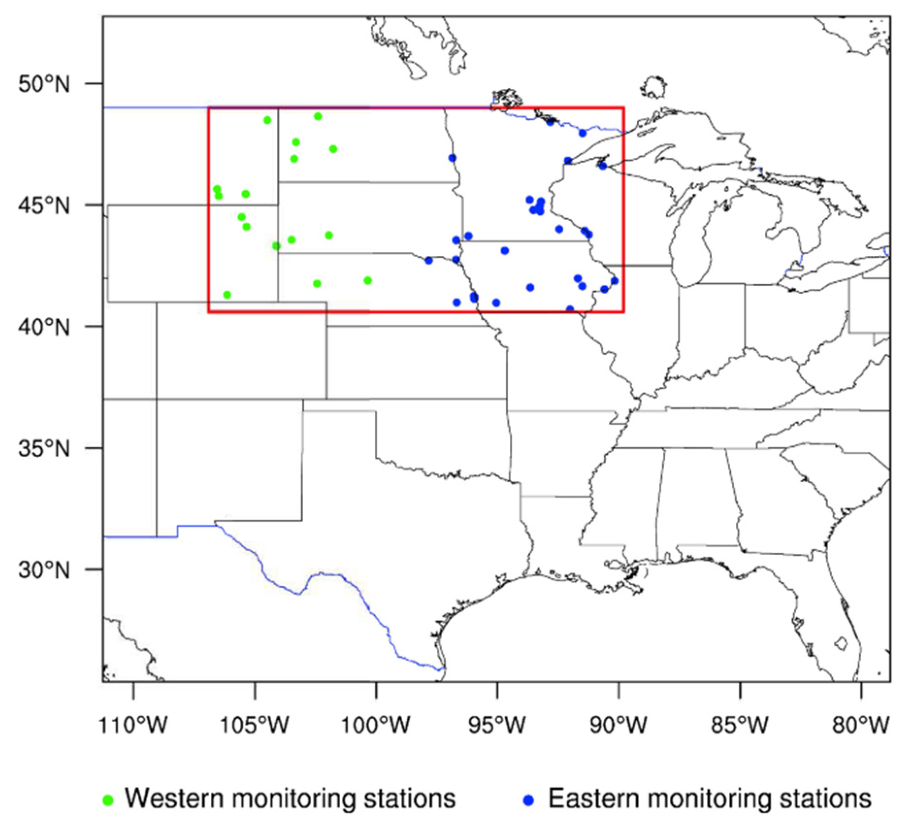
Figure 1. Modeling domain and location of hourly meteorology and air quality monitoring stations within the area of analysis centered on the Northern Great Plains.
Atmosphere 12 01121 g001
Figure 2. Hourly observed (Obs) and predicted (a) temperature at 2 m, (b) wind speed at 10 m, (c) surface pressure, and (d) relative humidity from RACM-MADE/SORGAM (RM), CBMZ-MOSAIC (CM), and MOZART-MOSAIC (MM) chemistry-aerosol mechanisms. Time series shown on left, with scatter plots of predicted vs. observed values on the right.
Atmosphere 12 01121 g002
Figure 3. Predicted maximum hourly O3 concentration (ppb) during July 2010. Model predictions for (a) RACM-MADE/SORGAM (RM), (b) CBMZ-MOSAIC (CM), and (c) MOZART-MOSAIC (MM).
Atmosphere 12 01121 g003
Figure 4. Monthly average of predicted hourly O3 concentrations (ppb) during July 2010. Model predictions for (a) RACM-MADE/SORGAM (RM), (b) CBMZ-MOSAIC (CM), and (c) MOZART-MOSAIC (MM). Mean bias of model predictions against observations for (d) RM, (e) CM, and (f) MM.
Atmosphere 12 01121 g004
Figure 5. Hourly observed (Obs) and simulated O3 concentrations (ppb) from RACM-MADE/SORGAM (RM), CBMZ-MOSAIC (CM), and MOZART-MOSAIC (MM) chemistry-aerosol mechanisms. Time series shown on left, with scatter plots of simulated vs. observed values on the right for (a) Fargo, ND and (b) Dickinson, ND.
Atmosphere 12 01121 g005
Figure 6. Monthly average of predicted hourly NO2 concentrations (ppb) during July 2010. Model predictions for (a) RACM-MADE/SORGAM (RM), (b) CBMZ-MOSAIC (CM), and (c) MOZART-MOSAIC (MM). Mean bias of model predictions against observations for (d) RM, (e) CM, and (f) MM.
Atmosphere 12 01121 g006
Figure 7. Hourly observed (Obs) and simulated NO2 concentrations (ppb) from RACM-MADE/SORGAM (RM), CBMZ-MOSAIC (CM), and MOZART-MOSAIC (MM) chemistry-aerosol mechanisms. Time series shown on left, with scatter plots of simulated vs. observed values on the right for (a) Fargo, ND and (b) Gillette, WY.
Atmosphere 12 01121 g007
Figure 8. Monthly average of predicted hourly PM2.5 concentrations (μg/m3) during July 2010. Model predictions for (a) RACM-MADE/SORGAM (RM), (b) CBMZ-MOSAIC (CM), and (c) MOZART-MOSAIC (MM). Mean bias of model predictions against observations for (d) RM, (e) CM, and (f) MM.
Atmosphere 12 01121 g008
Figure 9. Hourly observed (Obs) and simulated PM2.5 concentrations (μg/m3) from RACM-MADE/SORGAM (RM), CBMZ-MOSAIC (CM), and MOZART-MOSAIC (MM) chemistry-aerosol mechanisms. Time series shown on left, with scatter plots of simulated vs. observed values on the right for (a) Fargo, ND and (b) Gillette, WY.
Atmosphere 12 01121 g009
Figure 10. Monthly average of predicted hourly PM2.5 subspecies concentrations (μg/m3) during July 2010 for RACM-MADE/SORGAM (RM), CBMZ-MOSAIC (CM), and MOZART-MOSAIC (MM) mechanisms.
Atmosphere 12 01121 g010
Table 1. Physical and chemical parameterizations used in WRF-Chem model runs.
Option TypeSelected Option
Horizontal grid resolution24 km
Number of vertical layers28
Microphysics schemeMorrison [52]
Short & longwave radiationRRTMG [53]
Land surfaceNoah-MP [54]
Boundary layer schemeYSU [55]
Cumulus physicsGrell 3D [56]
Aerosol feedbackYes [49]
PhotolysisFast-J [57]
FDDA meteorology nudging6 h of spectral nudging at start of run
Chemistry schemeRACM, CBMZ, or MOZART
Aerosol schemeMADE/SORGAM, MOSAIC-4 bin
CHEM_OPT parameter43, 32, or 201
Meteorological data input2010 NARR, 32 km resolution
Biogenic emissionsMEGAN 2.04
Anthropogenic emissionsNEI-2011
Table 2. Statistical measures of model performance.
NameDefinition
Mean Bias (MB) i = 1 N ( M i O i ) N
Normalized Mean Bias (NMB) i = 1 N ( M i O i ) i = 1 N O i
Root Mean Square Error (RMSE) i = 1 N ( M i O i ) 2 N
Correlation
Coefficient (R)
i = 1 N ( M i M ¯ ) ( O i O ¯ ) i = 1 N ( M i M ¯ ) 2 i = 1 N ( O i O ¯ ) 2
Index i is one of N pairs of modeled and observed values, M are modeled values, and O are observed values.
Table 3. Statistical analysis of hourly meteorological variables during the month of July 2010 for the RACM-MADE/SORGAM (RM), CBMZ-MOSAIC (CM), and MOZART-MOSAIC (MM) chemistry-aerosol mechanisms. All stations considered have ≥90% of available hourly data.
Meteorology
Parameters
Obs.
Mean
Model
Mean
RMBNMBRMSE
Temperature (°C)
RM 23.30.800.42.23.1
CM22.923.40.800.52.33.2
MM 23.50.800.52.73.2
Surface Pressure (hPa)
RM 970.00.92−2.5−0.264.3
CM972.4969.90.92−2.5−0.264.4
MM 969.70.91−2.7−0.284.5
Relative Humidity (%)
RM 72.50.66−3.5−3.718.0
CM76.072.30.66−3.8−4.118.1
MM 71.80.67−4.2−4.718.2
Wind Speed (m/s)
RM 2.80.500.2311.7
CM2.62.80.490.2321.8
MM 2.80.480.2321.8
Table 4. Statistical analysis of predicted hourly O3 concentrations for the RACM-MADE/SORGAM (RM), CBMZ-MOSAIC (CM), and MOZART-MOSAIC (MM) chemistry-aerosol mechanisms. All stations considered have ≥90% of available hourly data.
O3 (ppbv)
Observed MeanSimulated MeanRMBNMBRMSE
East
RM 35.50.536.42313
CM29.234.40.565.32012
MM 36.10.566.92513
West
RM 38.20.483.81210
CM34.436.30.451.96.410
MM 37.60.453.21011
Average
RM 36.20.525.72012
CM30.534.90.534.41612
MM 36.50.536.02112
Table 5. Statistical analysis of predicted hourly NO2 concentrations for the RACM-MADE/SORGAM (RM), CBMZ-MOSAIC (CM), and MOZART-MOSAIC (MM) chemistry-aerosol mechanisms. All stations considered have ≥90% of available hourly data.
NO2 (ppbv)
Observed MeanSimulated MeanRMBNMBRMSE
East
RM 4.60.420.7194.3
CM3.94.40.420.5124.2
MM 4.50.410.6144.2
West
RM 1.40.36−0.8−222.2
CM2.31.40.35−0.9−282.2
MM 1.40.35−0.8−212.2
Average
RM 3.00.39−0.0−1.63.2
CM3.12.90.38−0.2−7.73.2
MM 2.90.38−0.1−3.83.2
Table 6. Statistical analysis of predicted hourly PM2.5 concentrations for the RACM-MADE/SORGAM (RM), CBMZ-MOSAIC (CM), and MOZART-MOSAIC (MM) chemistry-aerosol mechanisms. All stations considered have ≥90% of available hourly data.
PM2.5 (µg/m3)
Observed MeanSimulated MeanRMBNMBRMSE
East
RM 8.90.05−0.9−2.19.8
CM9.810.40.100.61311
MM 8.70.03−1.0−4.79.6
West
RM 3.60.05−1.2−175.2
CM4.83.50.11−1.4−185.3
MM 3.00.09−1.9−315.3
Average
RM 7.10.05−1.0−6.98.2
CM8.18.10.10−0.12.49.0
MM 6.80.05−1.3−148.1
Table 7. Statistical analysis of predicted daily average PM2.5 subspecies concentrations for the RACM-MADE/SORGAM (RM), CBMZ-MOSAIC (CM), and MOZART-MOSAIC (MM) chemistry-aerosol mechanisms. Comparison is carried out with daily average observation data collected every third day.
PM2.5
Subspecies
Observed MeanSimulated MeanRMBNMB
(%)
RMSE
EC (μg/m3)
RM 0.160.43−0.01−20.10
CM0.170.190.430.02200.11
MM 0.180.370.01100.10
OC (μg/m3)
RM 0.280.34−0.90−750.99
CM1.180.430.55−0.75−620.81
MM 0.760.42−0.42−360.67
NO3 (μg/m3)
RM 0.300.260.10200.38
CM0.200.570.280.371340.50
MM 0.550.260.351520.65
NH4 (μg/m3)
RM 0.75−0.010.26650.56
CM0.490.530.060.04110.37
MM 0.650.010.16250.57
SO4 (μg/m3)
RM 1.260.130.07301.0
CM1.180.53−0.15−0.65−370.84
MM 1.20−0.030.02320.88
Publisher’s Note: MDPI stays neutral with regard to jurisdictional claims in published maps and institutional affiliations.