1. Introduction
Determination of the coupling between the dynamic processes occurring in the lower atmosphere and subsequent changes in the ionospheric plasma parameters is one of the fundamental problems of the physics of the atmosphere. This work aims to establish the physical mechanisms of the disturbance energy transfer from the troposphere to the upper atmosphere and ionosphere. These disturbances include both regular events such as tides and passages of the solar terminator and irregular ones such as meteorological storms, earthquakes, and solar eclipses, etc.
According to experimental data [
1,
2,
3,
4,
5,
6,
7], the upper atmosphere and ionosphere response appear several hours after the disturbances occur near the Earth’s surface. The changes in the ionospheric plasma parameters caused by seismic events were observed several days or more before the earthquakes. They were characterized by an increase in the electron concentration over the epicentral region [
8,
9,
10].
Dynamic processes in the troposphere lead to a deviation of pressure, temperature, density, and chemical composition from the average values. Recently remote sensing methods using lidar measurements have become popular for studying the dynamics of the lower atmosphere [
11,
12,
13]. The main advantages of their use are a high spatial and temporal resolution of measurements and the possibility of long-term observations. Lidar sensing methods are based on the elastic scattering of laser radiation on the particles of the medium, including aerosols. The received scattered signal can be used to estimate the distribution and characteristics of aerosols, as well as the variations in atmospheric parameters.
The laser pulse passing along the sensing pathway is absorbed and scattered on the molecules and aerosols of the medium. A part of the backscattered radiation can then be collected and focused using the receiving equipment on a photodetector, which converts it into the electrical signal proportional to the incident light flux. Finally, the distance between the transmitter and the scattering objects along the sensing pathway can be unambiguously determined by the delay time from sending the laser pulse. The intensity of the received signal at each moment depends on the properties of the exact atmospheric scattering volume and the characteristics of the atmospheric sensing track along the double path from the laser source to the scattering object and back [
14]. Generally speaking, this type of remote sensing makes it possible to determine various parameters, e.g., the effective radii of aerosol particles, their volume concentration, the backscattering coefficient, and the refractive index of the medium, etc.
Existing hypotheses about the mechanisms of influence of the lower atmosphere on the conditions of the upper atmosphere and ionosphere are based on the concept of generation of atmospheric waves in the troposphere and their propagation vertically upward [
1,
9,
15,
16,
17,
18,
19,
20,
21]. The speed of propagation of various wave components depends on their frequency and spatial scales. This speed is much lower than the sound speed for low-frequency planetary and tide waves [
15]. The modelling of ionospheric seismic phenomena based on ideas about the propagation of medium-scale internal gravity waves (IGWs) from the epicentral region makes it possible to reproduce the amplitudes of ionospheric disturbances but does not explain their localization and stability during the period preceding the earthquake [
1].
In the present investigation, the primary attention is paid to IGWs with periods close to the Brunt–Vaisala period [
20], and as far as acoustic waves (AWs), which are excited in the troposphere. They can propagate almost vertically, and quickly reach ionospheric heights [
18,
21]. In the theoretical studies [
17,
18,
19], it was shown that nonlinear and dissipative processes accompanying the propagation of these AWs and IGWs lead to the formation of large-scale irregularities in the upper atmosphere and an increase in the influence of turbulent processes in the lower thermosphere. Small-time delays in the appearance of disturbances for various atmospheric layers, including their localization directly above the sources in the lower atmosphere, can also be explained based on gravity and infrasonic waves [
9,
19].
It should be noted that F-scattering and absorption in the D-layer are often observed during the monitoring of the ionosphere in periods of tropospheric disturbances. These processes have a significant impact on the determination of frequency characteristics, which are associated with changes in plasma parameters in the F-layer of the ionosphere [
22]. In recent years, methods developed for determining the total electron content (TEC) through analyzing signals received from the global positioning system (GPS) have become widespread in experimental studies of the ionosphere. Planetary TEC maps based on more than 6000 GPS receivers are worldwide and successfully used to study the dynamics of the ionosphere under various geophysical conditions [
23,
24]. For example, the features of the morphology of the equatorial ionosphere and the ionosphere disturbances during a solar eclipse are considered in [
25,
26]. As a result of observations and theoretical studies [
27,
28,
29,
30,
31,
32], it was found that propagation of AWs and IGWs upward from the region of meteorological disturbance has a significant effect on the ionosphere.
This study’s main goal was to experimentally confirm the previously proposed mechanism for transferring the energy of tropospheric disturbances that arise during the passages of the solar terminator and solar eclipse into the ionosphere due to the vertical propagation of acoustic and internal gravity waves. By simultaneous usage of lidar sounding and satellite GPS measurements in this work, we are able to estimate the vertical structure and localization of the wave source, as well as determine the characteristic response time of the ionosphere to various tropospheric disturbances.
The remainder of this paper looks as follows. The next section presents a lidar measurement technique. Here, we give a detailed description of the optical scheme of the two-channel analyzer of the receiving unit, the technical characteristics of the two-wave atmospheric Lidar LSA-2S, and the algorithm for processing the received reflected signal.
Section 3 is devoted to processing the results of satellite measurements. We describe there the method for the TEC reconstruction from GPS measurements. In particular, we apply a formula for determining the TEC from code measurements at two frequencies and describe a method for calculating the spectrum of the TEC variations.
Section 4 discusses in detail the features of the vertical propagation of AWs and IGWs in the atmosphere. For clarity, the data for calculating the vertical profile of the periods of propagating waves are given. The results and their discussion are presented in
Section 5. For that, we use data obtained simultaneously from lidar sounding and satellite GPS measurements during the passage of the morning and evening terminators, as well as during the solar eclipse. We also assess the wave source’s vertical structure and localization and determine the ionosphere’s characteristic response time to various tropospheric disturbances. At the end of this section, the influence of physicochemical processes in the D and E ionospheric layers on the formation of its response to tropospheric disturbances is discussed.
Section 6 concludes this article.
2. Lidar Measurement Technique
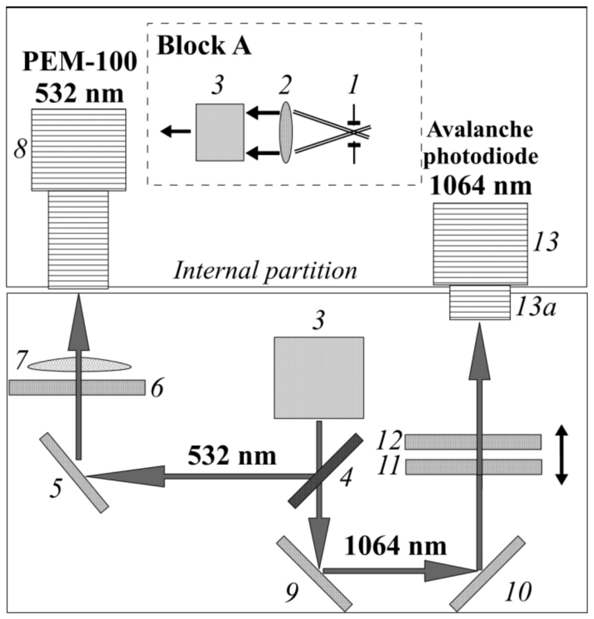
This paper presents the results of lidar sensing of tropospheric aerosols at KLGD station (Kaliningrad, Russia 54° N, 20° E). A two-wave atmospheric Lidar LSA-2S (Ltd. “Obninskaya fotonika”, Obninsk, Russia) was used for observations. The optical scheme of the two-channel analyzer of the receiving unit is presented in
Figure 1. The two-channel analyzer is designed to separate the light signal reflected by the atmosphere into single spectral components and register the separated light fluxes by photodetectors with subsequent transfer of information to the signal registration and processing system. The analyzer uses two types of photodetectors, i.e., PEM-100 photomultiplier in the 532 nm channel and the avalanche photodiode (AP) in the 1064 nm channel. In the plane of the input aperture of the analyzer (along the optical axis of the telescope), there is a flat plate with a set of apertures of the field of view combined with a collimating lens and a rotating mirror into one unit. Backscattered radiation passes from the telescope through the aperture of the field of view (
1). A collimating Fabry lens (
2), mounted behind the diaphragm, forms an almost parallel beam from the light collected by the telescope. This beam is turned by the mirror (
3) by 90° in the selectively reflecting spectral splitter (
4), which reflects radiation with λ = 532 nm and transmits radiation with λ = 1064 nm, thereby dividing the luminous flux into two channels. The radiation with λ = 532 nm reflected from the dielectric mirror (
5) enters the photomultiplier tube photocathode (
8) through the interference filter (
6) and the focusing lens (
7). Rotary dielectric mirrors (
9 and
10) direct radiation with λ = 1064 nm to the avalanche photodiode module (
13) through a filter unit consisting of a replaceable neutral filter (
11) and an interference filter (
12). Interference filters are used to separate backscattered signals from background solar radiation. A neutral filter is used to change the intensity of the light signal entering the avalanche photodiode. The image of the telescope’s main mirror is formed on the photocathode of the PEM and the photosensitive area of the AP using the focusing lens (
7) and objective (
13a) of the avalanche photodiode module, respectively. This ensures the constancy of the position of the illumination spot on the photocathode and the photosensitive area when changing the probing distance.
Lidar LSA-2S has the following technical characteristics: emitter is Nd:YAG-laser LS-2131 with two operating wavelengths of 1064 nm and 532 nm, with a pump energy of up to 25 J and a pulse repetition rate of no more than 20 Hz. The Cassegrain-type receiver with the main mirror of the receiving telescope is 260 mm in diameter, and a focal length of 1050 mm was used for backscattered radiation. The measurement time for one aerosol profile was no more than 15 min. The photodetector for the 1064 nm channel had a photocathode efficiency of 40% and an interfilter half-width of 3 nm. An FEU-10 photomultiplier with a photocathode quantum efficiency of 10% and a transmission half-width of 2 nm was used for the second channel at 532 nm.
The description of the algorithm for the automatic determination of aerosol parameters is given in [
33]. The algorithm is implemented in a software package for processing the LSA-2S measurement results using the parametric correlation dependencies between the integral characteristics over the aerosol size spectrum and the ratio of the backscattering coefficients at the indicated sensing wavelengths. As a result, this lidar made it possible to determine the characteristics of aerosols up to 10 km of altitude.
The intensity of the scattered lidar signal observed at the receiver is determined by the integral dynamics of the atmosphere along the path of the propagation beam with a length
where
c is the speed of light,
m is the number of strobes (maximum value is
m = 2000), and
is the pulse duration.
In general, the spectra of variations in tropospheric disturbances recorded in different channels should differ from each other because the intensity of the scattered lidar signal during sounding for both wavelengths depends on the size and parameters of the scattering aerosol. Nevertheless, the patterns of the spectra of variations can be similar if the lidar signal is reflected from a large-scale irregularity in the troposphere related to all types of aerosols. In this case, the length of the trajectory of the propagation ray,
, is related to the vertical distance,
h, from the Earth’s surface to the region of localization of the tropospheric irregularity by a simple relationship, i.e.:
where
is the angle of inclination of the laser beam to the horizon.
Spectral analysis of the time series obtained in the observations makes it possible to determine the frequency ranges of variations in atmospheric parameters at different altitudes. To study the dynamics of selected atmospheric layers, the function
F(t) is used, which is the difference in signal intensities for various strobes, i.e.:
Here, t is the time of the experiment, is the intensity of the scattered signal in the strobe with the m-th number. Next, the windowed Fourier transform of the function F(t) is applied. The duration of the observation analysis window is approximately equal to one hour. The spectra of atmospheric variations changing during the observations allow determining the contributions of the corresponding harmonics.
3. The Reconstruction of TEC from GPS Measurements
TEC is one of the key parameters of the ionosphere. There are several algorithms for TEC reconstruction, which are based on data from GPS receivers. For example, TEC can be determined from two-frequency phase measurements of pseudorange and code and phase measurements of pseudorange at the basic carrier frequency, as well as code measurements of pseudorange at two carrier frequencies.
Here we used the method for determining the TEC from the code measurements of the pseudorange at
MHz and
MHz GPS carrier frequencies. In this case, the group path of the radio wave is determined by the Davies formula [
34], i.e.:
where
is the group path for the frequencies
and
, respectively,
is the signal propagation time, and
D is the actual distance from the satellite to the receiver. The group refractive index,
, of signals at frequencies
and
in the ionosphere is defined as:
If we neglect the influence of the Earth’s magnetic field, then the refractive index,
, is defined by a simple expression [
34]:
Here,
is the local electron concentration. In this approximation, taking into account Equation (6), it is easy to obtain that:
Then, Expression (4) for pseudorange takes the form:
Here,
is the deviation of the receiver clock from the GPS time and
is the instrumental delay in the satellite and receiver equipment, including the measurement error. The second term on the right-hand side of Expression (8) is called the ionospheric range correction, which is determined by the ionospheric delay of the satellite signal at the carrier frequency,
f. Then, the value
is called the total electron content. Using Expression (8), written separately for two frequencies, it is easy to obtain a formula for determining the TEC from code measurements at two carrier frequencies, i.e.:
Here,
is hardware delay (
P-code ranging error), and the coefficient
M is defined as:
It should be noted that the hardware corrections for the satellite and the receiver change slowly over time and can be considered fixed during the diurnal observation period [
35].
In real observations at one of the ground GPS stations, simultaneous measurements of a set of differential delays,
, are carried out, where
i is the satellite number. The analysis of the group delay variation shows that the measured values,
, have a significant random spread [
36]. At some conditions, the dispersion can reach the value of 1–2 m. Its significant decrease is achieved by averaging over a certain time interval. In addition, there are still non-ionospheric variations,
. Therefore, one should use the maximum possible number of report,
, from various satellites with a large period,
T, to improve the accuracy of calculations. Because we were interested in the high-frequency component of TEC variations (with periods of 5–20 min), the spectrum of variations of the function
was determined as the difference between the current TEC variations obtained from observations with a step of 30 s and the smoothed ones with a smoothing window
T = 1 h. All spectra of TEC variations in this work were reconstructed from the data of satellite GPS observations at the mid-latitude station LAMA (Lamkovko, Poland, 53°53′ N, 20°40′ E), which is the closest to the location of the lidar sounding of the troposphere and is located at a distance of 85 km from the KLGD station.
4. Vertical Propagation of AWs and IGWs in the Atmosphere
As noted above, the features of the vertical propagation of acoustic and internal gravity waves significantly depend on their spatial and temporal scales. If we consider waves with a period of several hours, then the processes of AW and IGW propagation can be described by two-dimensional equations of hydrodynamics, which include the altitude and a horizontal coordinate. For a qualitative analysis of wave processes, isothermal atmosphere conditions are usually considered, whereas nonlinear and dissipative processes in the atmosphere are neglected. In this case, the requirement for resolving the equations of hydrodynamics is determined by the well-known dispersion relation [
20,
37], i.e.:
where
and
are horizontal and vertical components of the wave vector,
is the Brunt–Vaisala frequency, and
is the wave frequency. The scale height,
H, of the homogeneous atmospheric layer is represented as:
Here
is the Boltzmann constant,
is the neutral medium temperature,
is the molecular mass of atmospheric gas, and
g is the gravitational acceleration. The sound speed,
v, included in the last term in (13) has the form:
where
is the adiabatic index. Note that we have neglected the nonlinear and dissipative terms and the neutral medium temperature dependence on the altitude in (13).
It follows from (13) that the components of the wave vector,
k, can be simultaneously real (i.e., waves can propagate in an arbitrary direction) if one of the following two conditions is met:
or
Expression (16) determines the acoustic branch of wave processes. Value
is the lowest possible AW frequency and is called the acoustic cutoff frequency. The condition (17) determines the low-frequency branch corresponding to the IGWs, and the Brunt–Vaisala frequency,
, is the maximum possible frequency of IGWs.
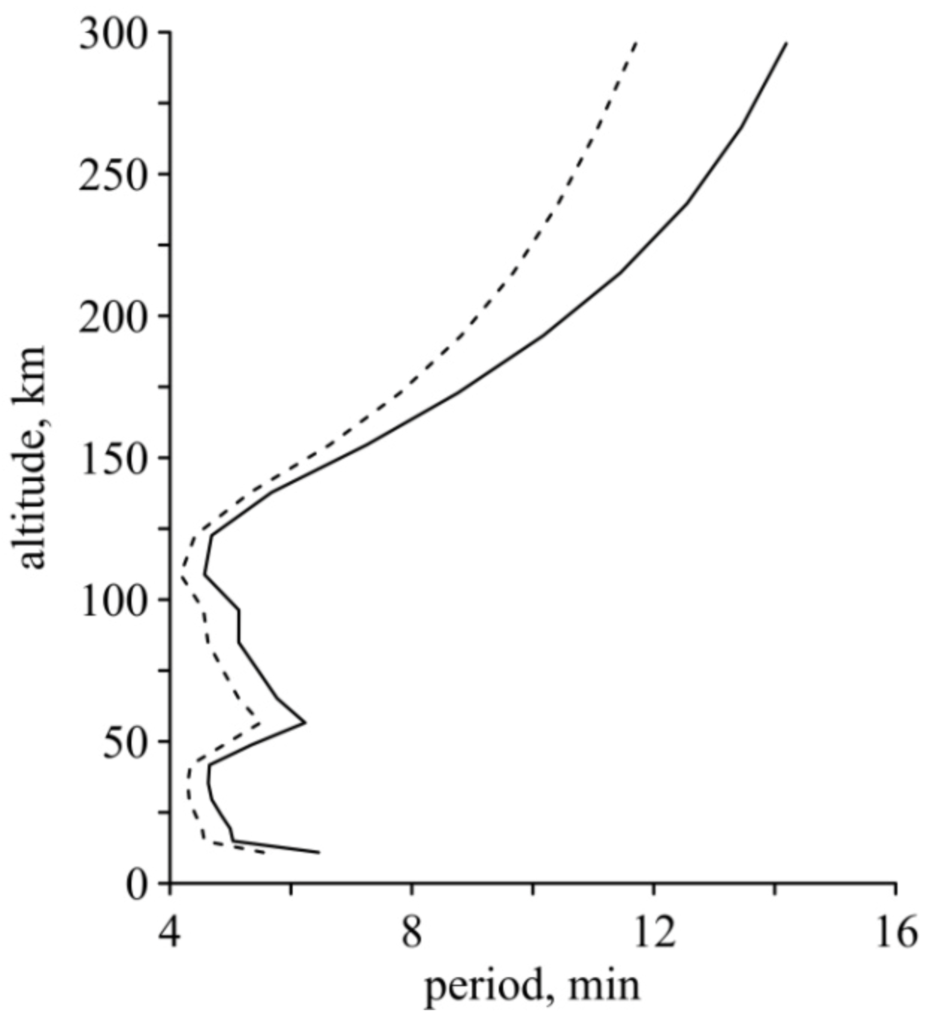
Figure 2 presents the vertical profiles of the wave periods corresponding to the Brunt–Vaisala frequency and the acoustic cutoff frequency. It can be seen that the time and frequency characteristics of AWs and IGWs propagating in the atmosphere depend significantly on the altitude.
It was shown in [
21] that, in the case of vertical propagation, AWs with periods of less than 4 min could reach the heights of the ionosphere. In addition, the authors of [
18] found that this is possible if AW deviates from vertical propagation by no more than 20°. Dissipative processes determine the limiting altitude of the AW propagation in the upper atmosphere. Indeed, there is a sharp change in their characteristics at altitudes exceeding 150 km [
39].
A more complicated situation arises if IGWs propagate with frequencies close to the Brunt–Vaisala frequency. This is primarily due to the change in the Brunt–Vaisala frequency with the altitude (see
Figure 2). Thus, the waves excited at tropospheric heights as IGWs can appear as AWs during their vertical upward propagation because the period of these waves may be less than the acoustic cutoff period at some altitude ranges. This effect can be observed, for example, in the mesosphere and the lower thermosphere.
The solution of the problem of the vertical propagation of IGWs with periods close to the Brunt–Vaisala period by analytical methods is practically impossible or involves significant difficulties. When the wavelength is much less than the scale height of the homogeneous atmosphere,
H, defined in (16), the approximate description can be used, which is valid for a homogeneous medium. If the spectrum of wavelengths significantly overlaps the
H value, splitting the atmosphere into the horizontal layers becomes necessary, considering its stratification to be exponential [
40,
41,
42,
43].
Theoretical studies using models describing the propagation of IGWs in the atmosphere in a wide frequency range make it possible to emphasize the main wave features. The propagation of these waves is accompanied by dissipative and waveguide processes that lead to the excitation of secondary IGWs [
2,
3,
31,
32,
38]. Because of this feature, the characteristics of disturbances created by spatially extended and mobile sources in the atmosphere get complicated. In particular, the increase in the periods of variations is observed, and the expansion of the perturbation region becomes comparable with the size of the source region. As a result, localized regions in the thermosphere are formed above the sources of disturbances located in the troposphere and near the Earth’s surface. In its turn, these areas affect the ionization balance in the upper atmosphere and lead to the ionosphere’s reaction to seismic disturbances, meteorological storms, the passage of the solar terminator, and solar eclipses, etc. Therefore, to study the ionospheric response to processes occurring in the troposphere, it is necessary to consider the spectral characteristics of variations in the parameters of the ionosphere (for example, TEC) during periods of noticeable disturbances of a various nature in the lower layers of the atmosphere.
5. Results and Discussion
We will now discuss the main results of this work concerning events occurring in the Earth’s troposphere, which lead to ionospheric disturbances. We are talking about the passages of the solar terminator and the solar eclipse. Both processes significantly affect the rate of heating/cooling of the troposphere. This is mainly due to the absorption of solar radiation by gaseous components of the troposphere, in particular, water vapor. Rapid changes in the tropospheric heating source initiate convective processes, which cause the appearance of sources of AWs and IGWs.
5.1. Ionospheric Disturbances during the Passage of the Morning Solar Terminator
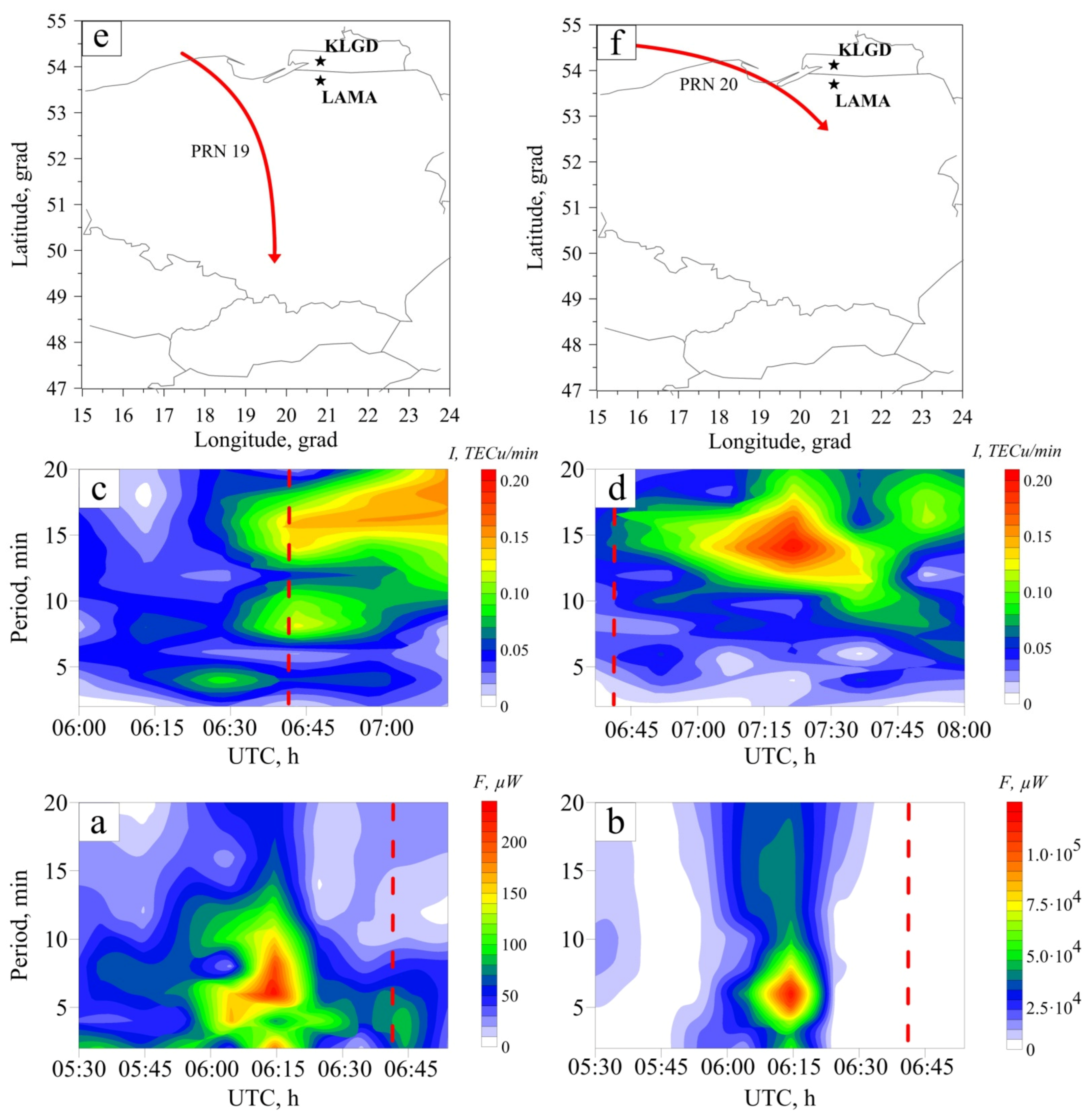
The solar terminator is a regular source of disturbances at all altitudes of the atmosphere. The lower horizontal panel in
Figure 3 shows the variation spectra related to the intensity of lidar signals scattered in the atmosphere with wavelengths λ
1 = 1064 nm (see
Figure 3a) and λ
2 = 532 nm (see
Figure 3b). The measurements were carried out at the KLGD station on 19 March 2012, during the morning solar terminator passing over the observation point (at 7:43 local time or 6:43 UTC). The preliminary analysis of the data shows that the best agreement of the spectra of intensity variations for both channels is achieved at a propagation beam length of
m, which corresponds to the localization of tropospheric irregularities at an altitude of
h = 2836 m (see (2)). From this figure, the increase in the amplitude of the intensity variations of scattered signals with periods of 5–7 min is observed approximately 30 min before the terminator passes.
The middle horizontal panel in
Figure 3 shows the spectra of TEC variations reconstructed from the data of satellite GPS observations at the mid-latitude station LAMA. The spectra were obtained as a result of processing signals received from two satellites, PRN 19 and PRN 20. During the passage of the solar terminator, the trajectories of the satellites were located above the observation station (see
Figure 3e,f), i.e., directly over the region of tropospheric disturbances (in the case of vertical measurements). The reconstructed data (see
Figure 3c,d) show that the reaction of the ionosphere to the tropospheric disturbances starts after 40 min and goes on for about 40 min. The main TEC disturbances have the characteristic period of 15–17 min and correspond to IGWs. At the same time, in
Figure 3c there is also a small contribution of AWs compared to IGWs at 6:45 UTC with a characteristic period of 8–10 min.
Note that the heating of the atmosphere is determined by the absorption of solar radiation, which depends on the density of the medium and the spectral composition of the radiation. Heating and ionization processes during the passage of the solar terminator in the thermosphere occur earlier than in the troposphere. However, the possibility of excitation of AWs and IGWs is determined by the conditions of the static stability of the atmosphere, i.e., temperature gradient. These conditions are different for the troposphere and thermosphere. In the troposphere, the temperature decreases with altitude; this is why there is an unstable equilibrium. In the thermosphere, on the contrary, the temperature rises with height above the region of absorption of solar radiation, which indicates a stable equilibrium. This fundamental difference determines the high probability of wave excitation during convective motions in the troposphere, while heating processes in the thermosphere will proceed more slowly and without excitation of AWs and IGWs.
5.2. Ionospheric Disturbances during the Passage of the Evening Solar Terminator
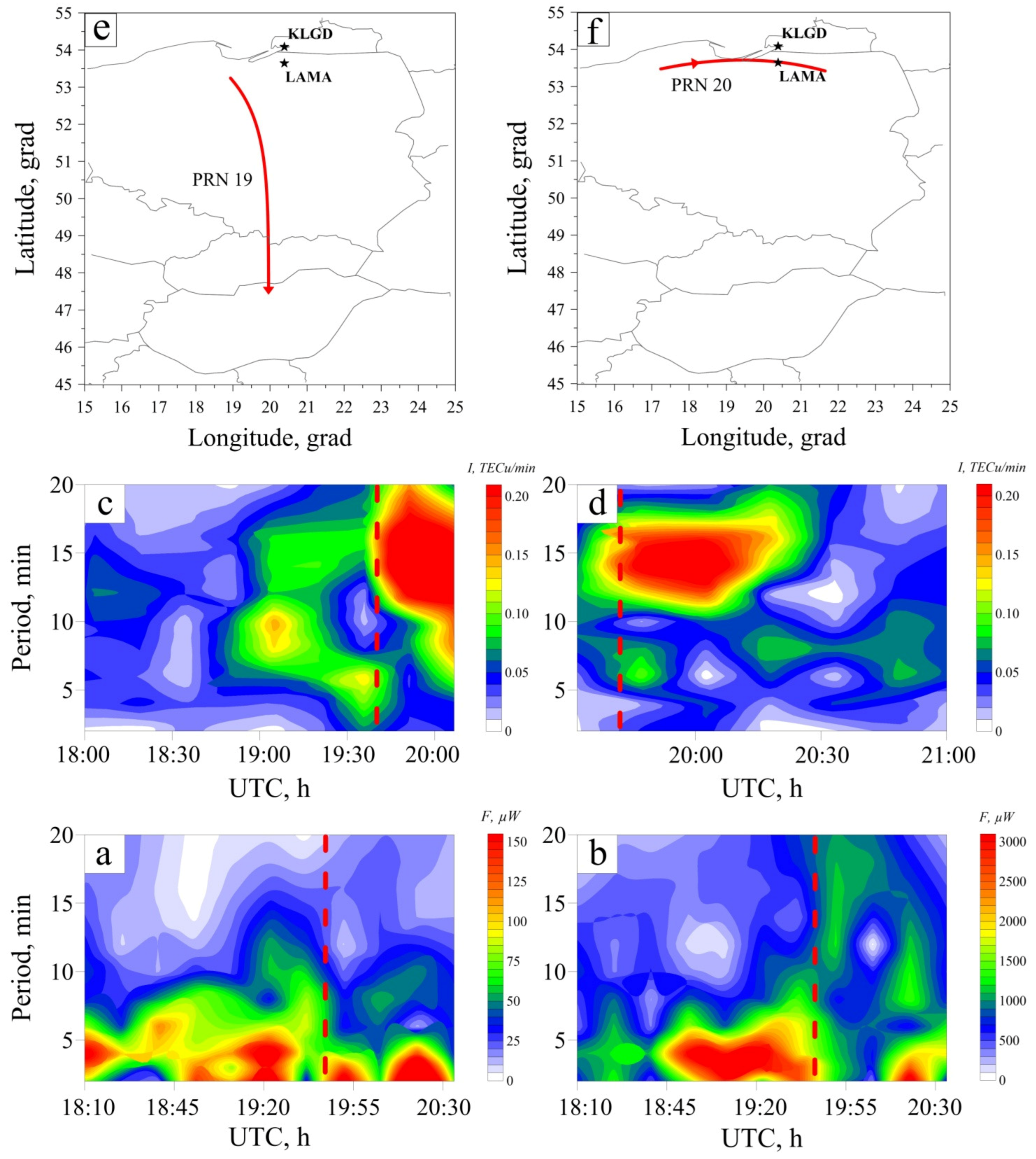
Lidar and satellite measurements during the evening solar terminator passing over the observation point (19:40 UTC) were carried out on 28 August 2012.
Figure 4 presents the spectra of the intensity variations of scattered lidar signals. An increase in the amplitudes of intensity variations with 3–5 min periods is observed approximately 45 min before the passage of the solar terminator at the altitude
h = 4255 m. The middle horizontal panel in
Figure 4 shows the spectra of TEC variations, reconstructed from the data of signals received from the PRN 19 and PRN 20 satellites. It can be seen that the time delay of the ionospheric response to tropospheric disturbances in the evening time is 40 min. The duration of ionospheric disturbances is just over half an hour. As in the morning, the main TEC disturbances have a characteristic period of 15–17 min.
5.3. Ionospheric Disturbances during the Solar Eclipse
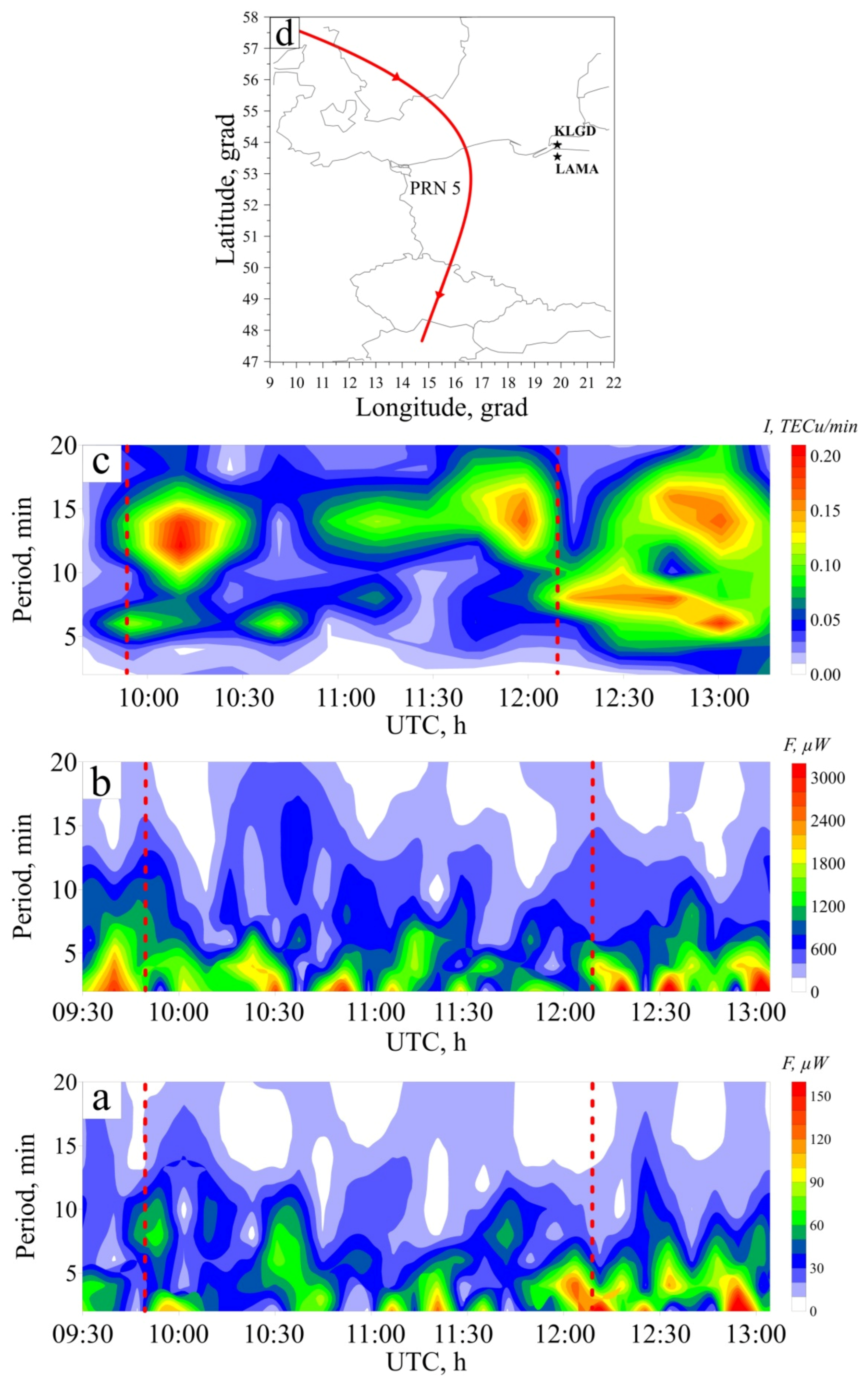
Measurements of tropospheric and ionospheric disturbances during the solar eclipse were carried out on 20 March 2015. The eclipse started at 9:50 UTC and finished at 12:10 UTC.
Figure 5 shows the spectra of variations in the intensity of lidar signals scattered in the atmosphere with wavelengths λ
1 = 1064 nm (see
Figure 5a) and λ
2 = 532 nm (see
Figure 5b). Here we present the results of measurements corresponding to the altitude
h = 3546 m. At the beginning of a solar eclipse, an increase in the intensity variations of scattered lidar signals with periods of 2–4 min is observed. Moreover, the feature is more pronounced in the channel with a wavelength of λ
2 = 532 nm. In the final phase of the solar eclipse, a slight increase in variations for both channels was observed 50 and 40 min before the end of the eclipse. A noticeable increase was observed 20 and 40 min after the end of the event.
It should be noted that the region of a solar eclipse is a mobile and spatially distributed source of disturbances in the atmosphere. Under these conditions, waves are excited that propagate both in the direction of motion of the region of disturbances and in the opposite direction [
32]. The resulting picture of the disturbances created by the eclipse region is a superposition of waves propagating in different directions. Therefore, it is natural to assume that the noted delays in the appearance of disturbances are determined by different propagation velocities of waves coming from the leading and trailing edges of disturbances in the lower atmosphere created by the eclipse region.
Simultaneous satellite observations (see
Figure 5c) show that the reaction of the ionosphere occurs 30 min after tropospheric disturbances and continues for about half an hour. The main TEC disturbances have a characteristic period of 12–15 min and correspond to IGWs. In the period from 12:00 UTC to 13:00 UTC, a small contribution of AWs with a characteristic period of 6–8 min is also observed.
In general, it can be noted that the response of the troposphere and ionosphere to a solar eclipse is pronounced both at the beginning and the end of the event. This is consistent with observations during the passages of the morning and evening solar terminators, but in this case, the picture is inverted because the events occur in reverse order. In the main phase of the eclipse, both tropospheric and ionospheric variations are less pronounced.
5.4. Geomagnetic Conditions during the Experiments
It should be noted that geomagnetic conditions are very important for performing this type of experiment. A quiet geomagnetic environment is a prerequisite for a perfectly clean experiment. Even weak geomagnetic activity can still cause strong and long-term disturbances in the thermosphere [
44], suggesting a potential effect on the TEC value. In this case, one should restore the TEC, excluding the influence of geomagnetic activity, and this is a significant problem.
On the selected days considered in the article, the geomagnetic activity, according to the IZMIRAN website (
https://www.izmiran.ru) (accessed on 30 August 2021), in the European part of Russia and Poland was low. Some concern could be caused by a magnetic storm on 17 March 2015, three days before the solar eclipse. However, post-storm effects usually develop as slow events continuing for several days. Therefore, they should not have been related to the observed
rapid changes in the state of the ionosphere.
5.5. Variations of Plasma Parameters in the D and E Layers of the Ionosphere under the Influence of Tropospheric Disturbances
It was shown in [
45,
46] that chemical reactions involving Rydberg states play a fundamental role in forming the ionospheric delay of radio signals. They include dissociative recombination, associative ionization [
47], exchange reactions in collisions of Rydberg particles with atoms and molecules of a neutral medium, and quenching of highly excited particles. A special role is assigned to the
l-mixing process [
48] because it is responsible for the formation of the quantum resonance properties of the medium for the propagation of radio signals. A detailed analysis of the influence of Rydberg states on the behavior of GPS signals in the D and E layers of the ionosphere is given in [
49]. The experimental confirmation of this fact is given in [
50].
Note that Expression (10) is used to minimize the systematic error for determining the TEC from code measurements at two frequencies. The factor
M defined in (11) is not accurate for accounting for the ionospheric signal delays. Its value depends on the concentration and temperature of slow electrons and neutral particles of the medium in the D and E ionospheric layers [
51].
Generally speaking, to correctly describe the dynamics of a two-temperature plasma under the action of tropospheric disturbances, it is necessary to consider the altitude distribution of slow electron concentration with energies up to 1 eV in the range from 60 to 110 km [
49]. Unfortunately, we did not have this necessary information during the experiment. Therefore, based on the available data, it is impossible to determine the exact position of the so-called
pierce point correctly. The information concerning only TEC is not enough to solve this problem. Additional measurements using sounding rockets or incoherent scatter radars are necessary. However, the time scales of ionospheric disturbances were determined quite accurately because we consider not the absolute values of the TEC but their variations in this work.
6. Conclusions
This paper presents the results of the simultaneous observations of tropospheric and ionospheric disturbances during the passage of the solar terminator and solar eclipse. Lidar observations showed that 20–30 min before the event, the disturbances of atmospheric parameters with periods of AWs and IGWs are generated in the troposphere. Analysis of the time series of tropospheric parameters shows that the duration of the disturbance depends on the degree of heating of the troposphere. In the colder troposphere (the passage of the morning solar terminator), the duration of the disturbance does not exceed 15 min. At the same time, in the heated troposphere (the passage of the evening solar terminator or the beginning/end of a solar eclipse), the disturbance lasts for about 40 min.
The vertical structure and localization of tropospheric disturbances also depend on the temperature of the environment. It was found during the experiment that, in the case of the morning terminator, when the absorption of solar radiation causes the heating of the troposphere, the maximum localization of disturbances is at an altitude km above the Earth’s surface. For the evening terminator, it corresponds to km. The vertical localization of tropospheric disturbances during the passage of a solar eclipse is rather arbitrary. It is observed only at the beginning and the final stage of the eclipse at an altitude of km, whereas in the main phase of the eclipse, the generation of AWs and IGWs is significantly weakened.
Simultaneous satellite observations demonstrate the response of the ionosphere (the TEC disturbance) to tropospheric disturbances. Analysis of the TEC time series allows us to assert that the characteristic response of the ionosphere occurs 30–40 min after the appearance of the tropospheric disturbance. In this case, the period of ionospheric disturbances is 15–17 min, and the duration does not exceed one hour.
We also note that the considered tropospheric disturbances can lead to additional failures in the operation of global navigation satellite systems caused by variations in plasma parameters in the D and E layers of the ionosphere [
51]. This statement primarily refers to the passage of the morning solar terminator, when the ionospheric response is particularly strong but short-lived (see
Figure 3).


 ,
, 
