Article

Sensitivity of Spring Phenology Simulations to the Selection of Model Structure and Driving Meteorological Data

1
Department of Meteorology, Eötvös Loránd University, Pázmány P. st. 1/A, H-1117 Budapest, Hungary
2
Excellence Center, Faculty of Science, Eötvös Loránd University, Brunszvik u. 2., H-2462 Martonvásár, Hungary
3
Faculty of Forestry and Wood Sciences, Czech University of Life Sciences Prague, Kamýcká 129, 165 21 Prague, Czech Republic
4
Department of Geophysics and Space Sciences, Eötvös Loránd University, Pázmány P. st. 1/A, H-1117 Budapest, Hungary
5
Centre for Agri-Environmental Research, School of Agriculture, Policy and Development, University of Reading, Earley Gate, P.O. Box 237, Reading RG6 6AR, UK
6
Centre for Agricultural Research, Agricultural Institute, Brunszvik u. 2., H-2462 Martonvásár, Hungary
*
Author to whom correspondence should be addressed.
Atmosphere 2021, 12(8), 963; https://doi.org/10.3390/atmos12080963
Submission received: 12 May 2021 / Revised: 22 July 2021 / Accepted: 24 July 2021 / Published: 27 July 2021
(This article belongs to the Section Biometeorology)

Abstract

:
Accurate estimation of the timing of intensive spring leaf growth initiation at mid and high latitudes is crucial for improving the predictive capacity of biogeochemical and Earth system models. In this study, we focus on the modeling of climatological onset of spring leaf growth in Central Europe and use three spring phenology models driven by three meteorological datasets. The MODIS-adjusted NDVI3g dataset was used as a reference for the period between 1982 and 2010, enabling us to study the long-term mean leaf onset timing and its interannual variability (IAV). The performance of all phenology model–meteorology database combinations was evaluated with one another, and against the reference dataset. We found that none of the constructed model–database combinations could reproduce the observed start of season (SOS) climatology within the study region. The models typically overestimated IAV of the leaf onset, where spatial median SOS dates were best simulated by the models based on heat accumulation. When aggregated for the whole study area, the complex, bioclimatic index-based model driven by the CarpatClim database could capture the observed overall SOS trend. Our results indicate that the simulated timing of leaf onset primarily depends on the choice of model structure, with a secondary contribution from the choice of the driving meteorological dataset.

1. Introduction

Plant development has evolved to respond to the seasonality of various environmental factors and is influenced by the interannual variability of climate [1,2]. Plant phenology research focuses on the periodic events occurring within the annual cycles of terrestrial vegetation [3,4]. Plant development has internal (genetic) and external (environmental) drivers. In the temperate zone, adaptive plant strategies must feature traits such as tolerance of late spring or early autumn frost damage and mid-summer water shortages. The timing of flowering and propagule development must enable successful reproduction [5].
In a feedback loop, the phenological stage of the vegetation influences the exchange of heat and mass between the land surface and the atmosphere [6]. Phenology thus plays an important role in ecosystem function, influencing the carbon balance of the soil–plant system and regulating biogeochemical and biophysical feedbacks through the coupled carbon-, water-, and energy cycles [4,6]. In the highly seasonal temperate zone at mid- and high latitudes, specific attention is paid to the start of the active vegetation period [2,7]. Surface and remote sensing observations provide information about the leaf onset at contrasting spatial scales [8,9,10].
Given the determinant role played by plant phenology, models of varying complexity have attempted to quantify the timing of the onset of the growing season (commonly referred to as the start of season (SOS), expressed by the numerical day of year (DOY)) [3,4,11,12,13,14,15,16]. Phenology models aim to capture the long-term mean SOS and its interannual variability [6], while an accurate representation of recently observed SOS trends related to climate change is also crucial for future prediction of plant growth [1,3]. Phenology models are integral parts of the biogeochemical models (BGMs), Dynamic Global Vegetation Models (DGVM), and also are increasingly included in General Circulation Models (also referred to as Global Climate Models, GCM) and Earth system models (ESM) [4,17,18]. Given the generalisation inherent in these large-scale models, their regional applicability and performance metrics of the methods they make use of remain a challenge [19].
Meteorological variables such as temperature, precipitation, radiation, and photoperiod are important drivers of vegetation development. These variables play a key role in phenology models [4,13,20,21]. During the past two decades, there has been a growth in the number of available meteorological datasets that can be used in studies of vegetation growth [22]. Data availability, however, poses new challenges: The decision of which dataset is the most suitable for the research is likely to affect the eventual result. Previous phenological studies used datasets developed by the Modern-Era Retrospective Analysis for Research and Applications (MERRA) [23], E-OBS [5], CRU-NCEP [2], ERA-15 reanalysis product of European Centre for Medium-Range Weather Forecasts (ECMWF) with a spatial resolution of 1° × 1° [24], and the ERA-Interim reanalysis of ECMWF [25]. The Daymet database [26,27], with 1 km spatial resolution, was also used for North America by a number of studies [13,20,28]. Surprisingly, given the large number of available datasets, a comparison of the performance of phenology models as a function of meteorological database selection is largely missing from the literature.
The aim of the present study is to quantify the sensitivity of SOS estimation to the choice of the model structure, and to the selection of the driving meteorological dataset. Three commonly used spring phenology models with different meteorology data requirements were used to evaluate the quality of phenological prediction as a function of the selection of driving variables. As a case study, we investigate Hungary, which has experienced a number of extreme weather events (heatwaves, drought, extreme precipitation) in recent years, likely to have affected the variability of SOS and therefore pose a modelling challenge [29,30,31]. We used the NDVI3g dataset as an observation-based reference [29].
We seek to answer the following questions:
  • How accurately can models simulate the observed SOS climatology in the region?
  • Are models able to capture observed interannual variability and long-term trends of SOS?
  • Is the choice of model or the choice of the meteorological database a more important factor affecting the accuracy of estimated SOS?
The results are very likely to inform the application of phenology models in Central Europe as the provided parameterisation can be directly included in BGMs or ESMs. The study also has global relevance as the tested comparison methodology applies to the study of any locality or phenological stage.

2. Materials and Methods
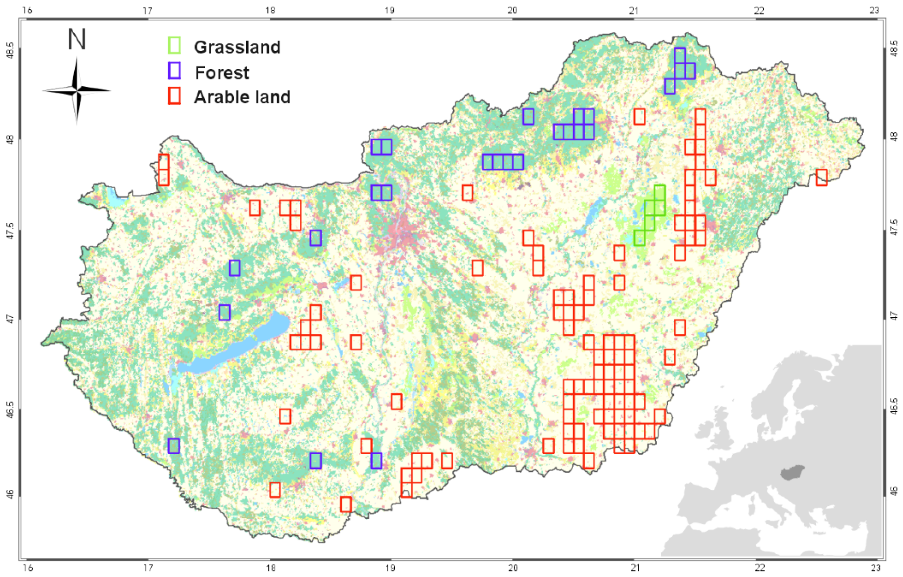
2.1. Study Area

This study focuses on Hungary (Figure 1). The country is located in the temperate climatic zone in Central Europe. Hungary is influenced by three major climate systems: Continental, Mediterranean, and Oceanic. The long-term (1981–2010) mean annual temperature is 10–11 °C, with mean annual precipitation of 500–750 mm. (https://www.met.hu/eghajlat/magyarorszag_eghajlata/; accessed on 11 January 2021.) The country is situated in the Carpathian Basin and is characterised by relatively low relief. The majority of the country is below 400 m with a mean elevation of ~150 m.
The dominant plant functional types (PFT) are arable land (~48% of the total country area), deciduous broadleaf forest (~18%), and grassland (~11%; [32]). Forests are typically found at higher elevations. The study uses a regular Gaussian grid with a 1/12° × 1/12° spatial resolution that was defined by the grid geometry of NDVI3g datasets (see Section 2.4).

2.2. Phenology Models

The estimation of the onset of spring vegetation growth is a highly scale-dependent task [17]. For large-scale modelling exercises, the species-specific or individual-based phenology models have to be upscaled to regional, continental, or global scales, which is a major challenge [6,17,20]. In this study, given the nature of the used models (BGMs, DGVMs, GCMs, and ESMs) we follow the method of [24] and [33] focusing on the climatological onset of leaf growth. In other words, we seek solutions that can be used to simulate climate-driven changes in the timing of SOS at a larger scale [20]. First, we handled SOS of forests, grasslands, and arable lands separately at the individual pixel level. Then we combined the PFT specific SOS according to the share of PFTs within the pixels to provide a single SOS for a given year that is comparable with the observation-based SOS at 1/12° × 1/12° resolution.
Three phenological models with different meteorological data requirements and underlying representation of the biological process were selected for the estimation of the onset of spring leaf growth.

2.2.1. WM

The first phenological model uses the simplest (and probably the most popular) approach: SOS is determined by accumulated thermal time. This method is widely used in terrestrial models such as IBIS (Integrated Biosphere Simulator; [34]) and CLM-DGVM (Community Land Model–Dynamic Global Vegetation Model; [34]). In this model (referred to as the warming model; WM), SOS is estimated as the calendar date when the cumulative growing degree-day (GDD; also known as heatsum relative to a predefined base temperature) exceeds a predetermined value. For a given PFT-specific base temperature, WM has one adjustable parameter, which is the cumulative GDD threshold. We use 1 January as the start of the GDD accumulation. The base temperature (Tbase) and GDD threshold values used in this study were set by model optimisation (see Section 2.6). WM uses mean daily temperature only as input data.

2.2.2. CWM

The second model uses heat accumulation in spring as the driving factor (just as in the WM), but the timing of SOS as also affected by the exposure to low temperatures (i.e., fulfilment of the chilling requirement, or in other words vernalization) during winter. In this model, the GDD threshold is defined as:
GDD ( t ) = a + b · e c · NCD ( t ) ,
where NCD is the number of chilling days, while a, b, and c are three adjustable model parameters. Here we refer to this model as a chilling-warming model (CWM). This approach is used in the process-driven ORCHIDEE (Organizing Carbon and Hydrology in Dynamic EcosystEms; [34]) and the SEIB-DGVM (Spatially Explicit Individual Based-Dynamic Global Vegetation Model; [34]) models. The CWM uses daily mean temperature as the input, but in this case, estimates of SOS for a given year use meteorological data from the second half of the previous year to calculate the fulfilment of the chilling requirement. Parameter optimisation was performed before the application of the model.

2.2.3. GSIM

A bioclimatic index (Growing Season Index; GSI) was constructed for the third model (Growing Season Index Model, GSIM), representing known constraints to foliar development [35]. Three variables were combined to jointly modulate the timing of SOS (where each variable has two limits): Suboptimal (minimum) temperature (with limits TMmin and TMmax), vapor pressure deficit (VPD, with VPDmin and VPDmax), and photoperiod (Photomin and Photomax). Threshold limits, potentially adjustable in the GSI model, were set, and then indices were calculated separately for all three variables, and the GSI was calculated by multiplying the three indices. The calculated GSI has to reach a threshold, which is also an adjustable parameter. There is an additional adjustable parameter in the model that controls the smoothing window size that is used to avoid false onset detections [35]. Optimisation of the GSIM was done for all eight parameters included in the model.

2.2.4. Applicability of the Models

In forests and low-management intensity grasslands, it is reasonable to assume that the meteorological variables are the main drivers of the SOS date. In arable crops, particularly in spring-sown varieties, the phenology is also affected by human decisions (e.g., planting date). The often-intensive spring leaf growth of winter crop varieties is largely driven by the environmental conditions of the current and preceding years, as they are planted in autumn and are overwintering. Winter crops typically require vernalization; the accumulation of exposure to cold temperatures affects their phenological development [36,37]. In this sense, the CWM (originally developed for simulation of bud break of trees) might be structurally more suitable for winter crops and might reflect the effect of environmental variables on the spring leaf growth. To further complicate the picture, actual environmental conditions affect farmer decision making [38]. Crop phenology thus integrates weather, variety, and anthropogenic factors. At the target resolution of the study (1/12° × 1/12°), winter and spring varieties share the total harvested area within a pixel almost equally (http://www.ksh.hu/docs/eng/xstadat/xstadat_annual/i_omn007a.html, accessed on 20 January 2021). Since spring varieties are typically planted after the initiation of leaf growth of other vegetation types, the phenology of winter crops may be the main driver of the observed green-up within a pixel. In summary, we assume that the climate will affect the intensive spring leaf growth for all plant functional types, and theoretically, all three model types are suitable for the estimation of SOS.

2.3. Meteorological Datasets

2.3.1. CarpatClim Database

CarpatClim is a high-resolution dataset based on weather observations of several meteorological variables for the Carpathian Region (44°–50° N latitudes and 17°–25° E longitudes) covering the period of 1961–2010 [39] at a 1/10° × 1/10° resolution regular grid. CarpatClim uses a relatively dense observation network (in Hungary, 109 stations measured precipitation and 34 stations temperature), although its temporal coverage is limited (the dataset ends in 2010). CarpatClim is one of the regional, observation-based gridded datasets that are available for specific parts of Europe (summarized in [22]). 1/10° × 1/10° resolution of CarpatClim data were interpolated to the target 1/12° × 1/12° resolution grid of this study using simple linear interpolation taking into account the area of the grid cells overlapping with the target grid cells.

2.3.2. FORESEE Database

FORESEE (Open Database FOR Climate Change-Related Impact Studies in Central Europe) is a free meteorological database for Central Europe covering the period of 1951–2100 with 1/6° × 1/6° spatial resolution [30,40]. FORESEE contains observation-based daily minimum/maximum temperature, precipitation data, and climate projections for these variables—the latter starting from the last continuously updated observed year. The dataset is supplemented by daylight mean temperature, global radiation, and VPD data estimated by the MTClim model [26]. Daylength (photoperiod) is also estimated by MTClim and used in this study to drive the GSIM. The target area of FORESEE spans 42°35′–51°05′ N latitudes and 10°55′–28°05′ E longitudes. The observation-based data (1951–2018) were built using the E-OBS v17 dataset [29,41]. FORESEE uses a relatively low number of station data (17 stations for temperature and 16 stations for precipitation). In the present study, we used a version of FORESEE interpolated to the target 1/12° × 1/12° resolution regular grid defined by the reference dataset.

2.3.3. ERA5 Database

ERA5 is a reanalysis database constructed and disseminated by ECMWF [42,43]. At present, ERA5 contains data from 1979 (also preliminary from 1950) until the present in hourly time steps. Observations are used indirectly in ERA5 through the 4D-Var data assimilation method. In this sense, ERA5 represents an alternative compared to CarpatClim and FORESEE that are both interpolated observation-based datasets. This assimilation method uses instrumental measurements and short-range model runs to produce gridded values of several meteorological parameters. The horizontal resolution of ERA5 is 1/4° × 1/4°. Surface data are available for 2D meteorological parameters such as rainfall, 2m temperature, wind speed, incoming solar radiation, and many others. ERA5 data were retrieved using the CDS API via R interface at a regular 1/10° × 1/10° resolution grid (due to technical considerations). The hourly data were post-processed to provide daily minimum/maximum temperatures and other ancillary variables needed in the study. ERA5 data were interpolated to the target grid using simple linear interpolation taking into account the area of the grid cells overlapping with the target grid cells.

2.4. Remote Sensing Based Reference Spring Phenology Dataset

Satellite-based remote sensing data were used in the present study to provide a reference for modelling. As remote sensing does not directly measure the SOS, the information registered by the instruments can be considered as proxy data. Thus, SOS determination from satellite data also has its own methodology and uncertainty (e.g., [44,45,46,47,48]) that has to be considered during the application of the datasets.
The MODIS-adjusted NDVI3g remote sensing dataset [29] covering Central Europe was used to provide observation-based data describing SOS. The dataset was created from the original NDVI3g [49] by statistical harmonisation (adjustment) using NDVI calculated from the data measured by the MODerate resolution Imaging Spectroradiometer (MODIS). Adjustment coefficients were determined for the overlapping years of NDVI3g and MODIS (2000–2013) and then applied to the entire NDVI3g period (1982–2013). The dataset has a 1/12° × 1/12° spatial and 15-day temporal resolution for the 1982–2013 period. The harmonised NDVI3g dataset showed improved quality for diverse vegetation metrics compared to the original NDVI3g [29].
SOS was calculated at pixel level based on the methodology described in [29], which partially follows the work of [50]. In brief, SOS was calculated as the average of three different methods, where SOS is the date when (1) the NDVI shows the highest rate of change in the year; (2) the derivative of the wavelet transformed function fitted to NDVI values reaches its first local maximum; and (3) the NDVI first reaches the value that gives the highest rate of change of the multiannual NDVI curves (serving as a predefined threshold). The uncertainty of the NDVI3g-based reference SOS data was estimated as the standard deviation of the results of the above three methods.

2.5. Ancillary Data Used in the Study

The elevation of grid cells at 1/12° × 1/12° resolution was estimated by the Shuttle Radar Topography Mission (SRTM) Digital Elevation Database [51]. Elevation classes within the target area were created considering the number of pixels within a given class so that sufficient data were available to support statistical analysis. Three classes were created: pixels below 100 m, between 100 and 200 m, and above 200 m elevation.
The share of generalized land cover categories (i.e., PFTs) within each grid cell was calculated based on the CORINE Land Cover 2012 database. Grid cells with relatively homogeneous PFT cover were used for the optimisation of the phenology models. Pixels were classified into three categories: If, within the pixel, PFT cover reached 70% threshold for grasslands, 80% threshold for forests, and 90% threshold for arable lands. Overall, 25 pixels were selected for forest, 99 pixels for arable lands, and only 5 pixels for grasslands (Figure 1).

2.6. Optimisation of Phenological Models

Annually calculated, PFT-dependent median SOS dates were used to optimize the models using the selected homogeneous pixels and the description of their spring phenology from the NDVI3g dataset.
In the case of the WM, a simple global search algorithm was used with Tbase limit ranging from 0 to 8 °C and GDD threshold ranging from 100 to 300 °C days. We used 1 °C steps for Tbase and 1 °C days steps for GDD threshold, and all parameter combinations were tested. The root mean square error (RMSE) was calculated from the SOS medians of the PFT specific pixels calculated by model–dataset combinations and the NDVI3g-based SOS median. The parameter optimum was selected by finding the minimum RMSE.
In the case of the CWM, all five parameters were subject to calibration (a, b, c, GDD, and NCD; see [24]). We set the range of the parameters based on [24,34]. Parameter a was varied between −90 and −47 °C days, while parameter b was varied between 622 and 653 °C days, with 1 °C days steps for both cases. Parameter c was varied between −0.011 and −0.0101 with 0.001 steps. Tbase was varied between 0 and 8 °C, and NCD_Tbase was varied between 0 and 5 °C with 1 °C steps (NCD refers to the number of chilling days).
The GSIM model is characterised by a relatively high number of parameters. To simplify the optimisation process, we first fixed the difference between the TMMin and TMMax (see above). Then, minimum temperature limits were varied systematically between −2 and 7 °C (TMMin), and 5 and 14 °C (TMMax) with 1 °C resolution. VPD limits were varied between 500–1400 hPa (VPDmin) and 3700–4600 hPa (VPDmax) with 100 hPa steps. The photoperiod was varied between 35,500–36,400 s (PhotoMin) and 39,100–40,000 s (Photomax) with 100 s steps. After this initial optimisation, a second step was necessary with reduced degrees of freedom. By fixing all other parameters, minimum temperature limits were varied between −3 and 5 °C (TMMin), and 3 and 11 °C (TMMax) with 0.5 °C resolution, now without fixing the difference between the minimum temperature thresholds. The GSI threshold was also included in the optimisation and was varied between 0.42 and 0.58 with 0.01 steps.
After model optimisation using relatively homogeneous PFT cover pixels, phenological models were run for all available pixels in the target area. Then the PFT-specific results were combined by weighting using the share of PFTs for the given pixel. The resulting SOS dataset reflects the contribution of different PFTs to the estimated SOS, which means that they are comparable with the observation-based SOS dataset for the whole country.

2.7. Statistical Analysis

The SOS datasets generated using the models and the adjusted NDVI3g dataset were calculated in a common 1/12° × 1/12° resolution grid, with a total of 1592 pixels available in Hungary. As the NDVI3g dataset provides unrealistic values over lakes and urban areas, a few pixels were excluded from the analysis. The remaining 1539 pixels were analysed in the study for the period of 1982–2010. The start year of the comparison is defined by the availability of NDVI3g, while the end year (2010) is constrained by the limited temporal availability of the CarpatClim dataset.
Climatological maps providing information about the long-term mean SOS data for the pixels were created. Long-term mean SOS was calculated for each pixel using the different model–database combinations, and for the NDVI3g dataset. The pixel-based results were further analysed (country median, standard deviation, 5th and 95th percentiles). Elevation classes were created for analysis based on the DEM dataset. We also calculated the spatial covariance between the pixel level SOS climatology values.
The interannual variability of the results was quantified in annual box-whisker plots. Median SOS dates were used to further analyse the relationship between the observation-based and estimated data. Performance metrics (bias, RMSE, and square of the linear correlation coefficient (R2); for definitions see e.g., [52]) were calculated using the annually calculated country medians for the elevation classes, and the pixel-based SOS time series as well.
Trend analysis was performed using the calculated annual median SOS values to check the applicability of the models in terms of long-term, climate change-related SOS shifts in the study period. The analysis was executed at the pixel level, then histograms were created to compare the overall, pixel-based trends, and the observation-based trends. Statistical significance (p-value) of the regressions was quantified.
To quantitatively assess whether the model selection or the meteorological database selection influences the results more, a specific algorithm was developed. Annual SOS dates were analysed for the 1982–2010 period for all nine model-database combinations at the pixel level. As the first step, cumulative density functions (CDFs) were calculated for the SOS time series of the given pixel. Two groups were created from the CDFs, where each group contained three separate CDF combinations. In the first group (weather group), the three models were fixed one at a time and their results were compared as the function of meteorological datasets (CarpatClim, FORESEE, ERA5). In the second group (model group) the three meteorological datasets were fixed one at a time, and the associated model results were compared for the WM, CWM, and GSIM models, respectively. A total of six CDF combinations were created (three for the weather group and three for the model group), where each combination consisted of three CDFs. The Kolmogorov–Smirnov distance was used to calculate the average distance between all possible CDF pairs in each combination. The mean distance was calculated for the two groups (model and weather). Then, to calculate one unified index (referred to as the Importance Indicator, abbreviated as IID) the mean distance of the second group was subtracted from the mean distance of the first group. If the model selection is more important than the meteorological dataset selection, the difference is negative. The IID was calculated for all grid cells and visualised in the form of a heat map. The statistical significance of IID was calculated with a permutation test for each pixel. Using the previously calculated CDFs, 100,000 permutations were performed. We calculated the IID for each relabelled CDF. The null hypothesis was that the true IID is zero (i.e., we cannot choose between model and weather group). The p-values were calculated by counting the number of cases where the absolute value of the random IID was higher than or equal to the absolute value of the actual IID.
The calculations were performed in Interactive Data Language v8.5 (Harris Geospatial Solutions, Inc., Broomfield, CO, USA), and in the R statistical computing software [53], where the latter was used for IID calculations.

3. Results

3.1. Model Parameterisation

Table 1 presents the parameters of optimised models. As a result of the GSIM optimisation, the minimum temperature and VPD thresholds were changed relative to the original values proposed by [35], while the daylength limits remained the same. For grasslands and arable lands, the minimum temperature limits are the same, and for forests and grasslands, VPD limits became the same.
For the WM, the optimum GDD threshold was set to 105–128 °C days (depending on the PFT) as a result of the calibration. The same Tbase was used for grasslands and arable lands (5 °C). Tbase for forests is higher than that of arable lands and grasslands.
Tbase values used by the WM and the CWM differ as a result of the optimisation. However, the Tbase values for grasslands and arable lands are lower than for forests, both for the WM and CWM models. The chilling day base temperature (NCD_Tbase) is lower in grasslands than in forests and croplands.

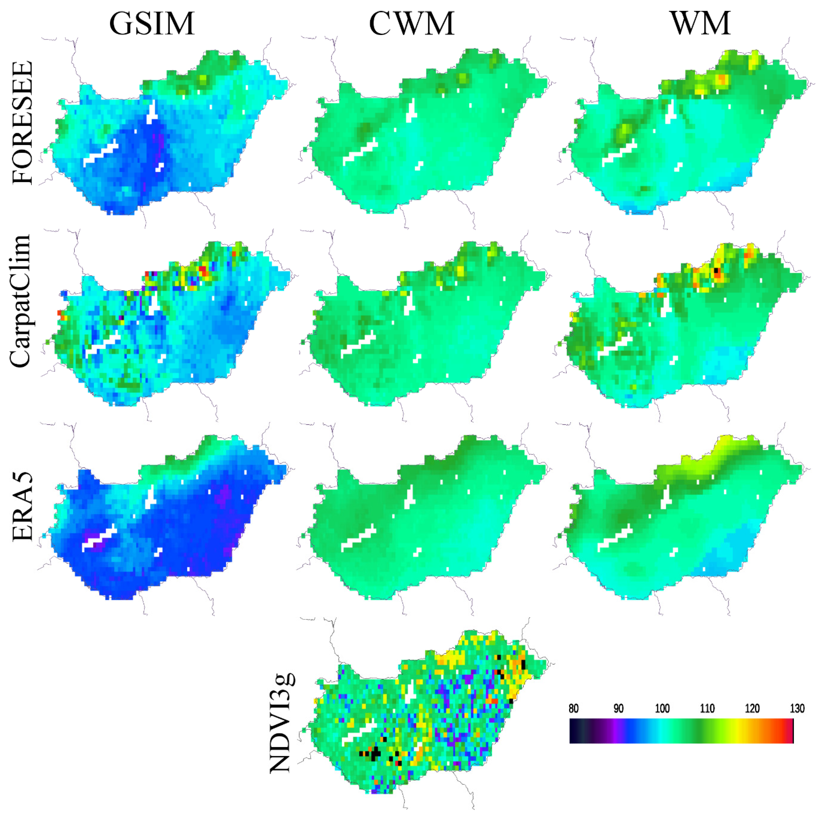
3.2. Climatology Maps for SOS

Figure 2 shows SOS climatology maps for the country, calculated as median SOS date (DOY) of the three models driven by the three different climate datasets covering the 1982–2010 period. Model results disagree about the location of regions typical for early SOS. Observation-based long-term SOS indicates the earliest greening in the eastern, plain regions of the country. If we compare the sensitivity of the models to local features, it is clear that the CarpatClim dataset provides the highest level of details (pixel-by-pixel variability). As expected, the ERA5 dataset is characterized by smoothed-out spatial features, given the 1/4° × 1/4° native spatial resolution, which is quite coarse compared to the other datasets.
Table 2 provides key statistics behind the SOS climatology maps, allowing for quantitative insight into the spatial variability of the SOS estimates. The observation-based median SOS date for the 1982–2010 period is DOY 105 (15 April). SOS values increase with elevation both according to the models and the observation (with the exception of FORESEE-driven GSIM and ERA5-driven WM). Model–database combinations typically reproduce the observed median given the optimisation of the models. GSIM systematically predicts earlier SOS relative to the observation, except for the CarpatClim input data in the 200–700 m elevation class. In the case of CWM and WM, the different meteorological datasets provide very similar results.
Standard deviation (i.e., spatial variability) is underestimated by the model–database combinations (except for the GSIM and WM driven by CarpatClim in the 200–700 m elevation class). The CWM consistently predicts smaller spatial variability than the other two. The GSIM has the highest overall SD values; these are the closest to those of the observations but still underestimated (the exception is the 0–100 m GSIM driven by the CarpatClim and ERA5 database). According to the observed data, the earliest vegetation onset is DOY 92 (2 April), while the latest is DOY 118 (28 April). Looking at model performance, the GSIM is the best in estimating SOS data points in the 5th percentile (early greening regions), while the WM provides better predictions for the 95th percentile (late greening regions).
An additional statistical assessment of the SOS climatologies is presented in Table S1 of the Supplementary Material. According to the results, the spatial covariance between the maps generated by the model-database combinations is typically low. The highest R2 is associated with the WM driven by the CarpatClim and the FORSESEE database.

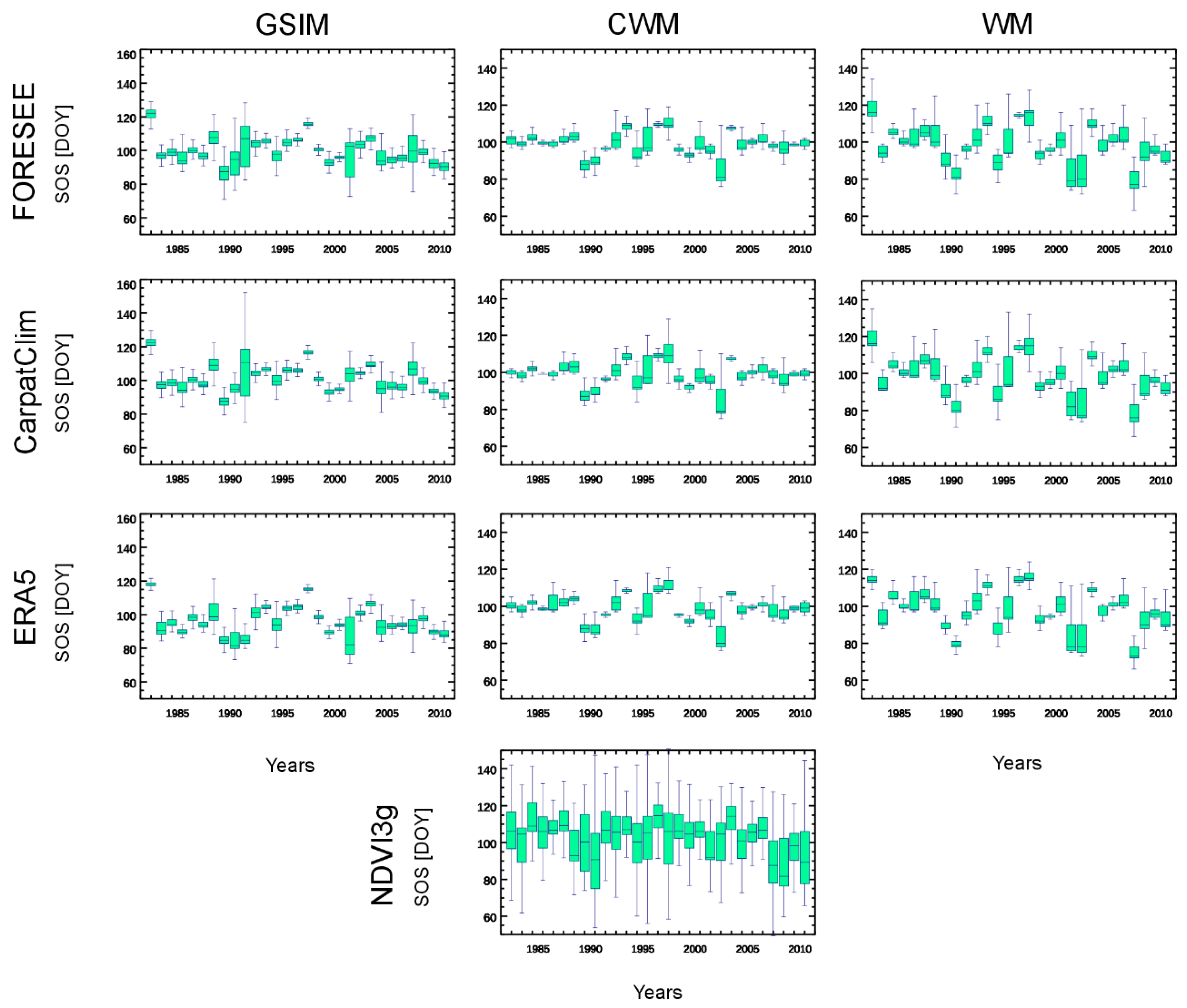
3.3. Interannual Variability
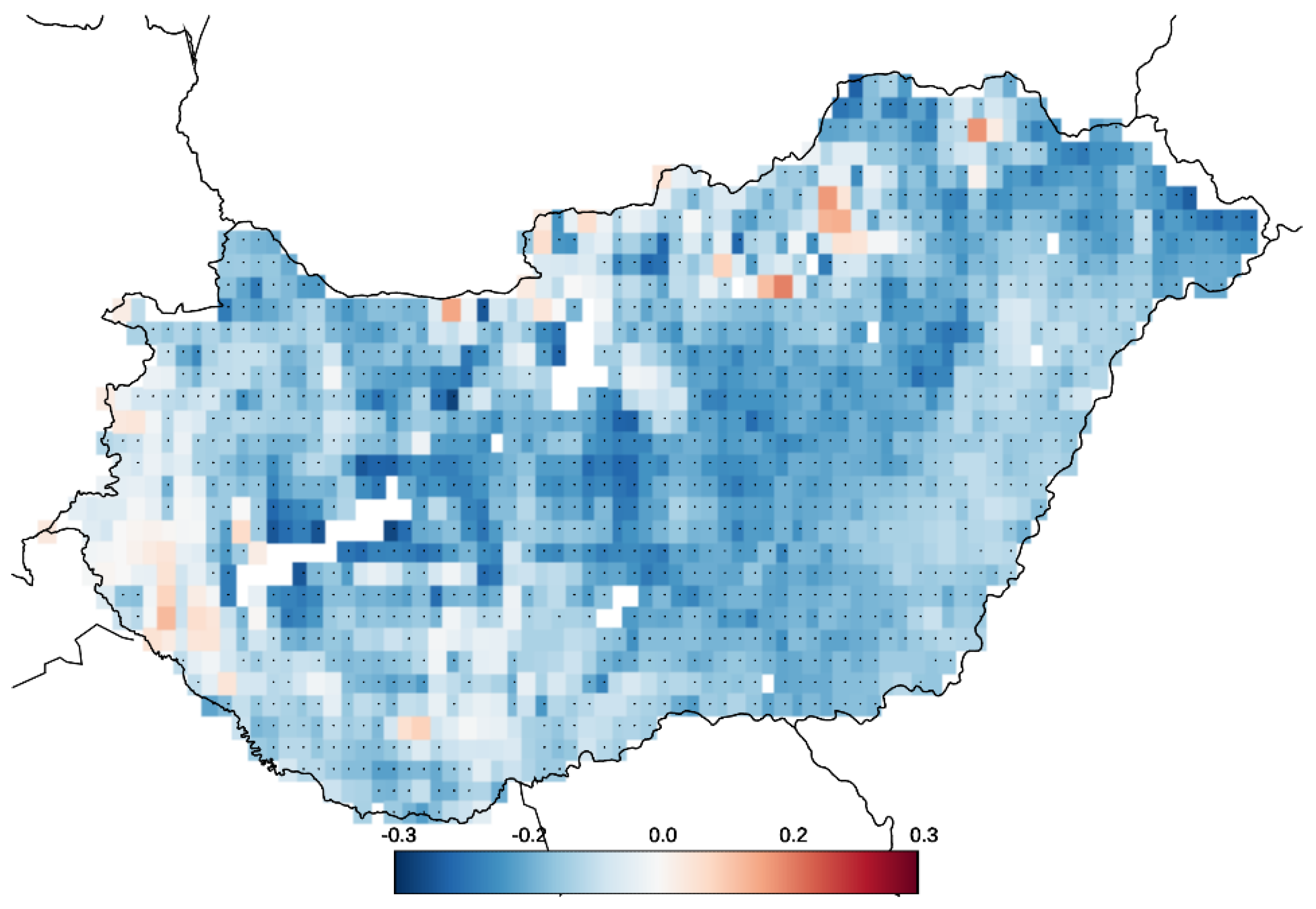
Figure 3 shows the interannual and spatial variability of the modelled and observed SOS, with relatively higher spatial variability within the specific years for the GSIM and the WM. CWM is associated with low spatial variability across years that is consistent with the SOS maps presented in Figure 2. None of the model-database combinations could reproduce the observed high spatial variability of SOS (represented by the interquartile ranges) for the specific years that are present in the observation-based SOS plot (lowest graph in Figure 3).
IAV was expressed as the standard deviation around the annual median SOS dates. Table 3 shows statistics about the IAV for the whole county, based on all available model-database combinations, and also for the NDVI3g-based results. The overall standard deviation of the observation is ~5 days and decreases with elevation. The observed IAV is smaller than modelled, and the CWM estimate is the closest to the NDVI3g-based IAV. In the case of WM, the CarpatClim-driven CWM and ERA5-driven GSIM concur that the least variability is found at the elevation class 200–700 m, which is the case in the observed data.
The performance metrics describing modelled annual median SOS dates relative to the observation-based dataset show that the models typically slightly underestimate the observation. Further, the smallest overall RMSE value results from the CWM, followed by WM and GSIM (Supplementary Material, Table S2). An additional statistical assessment of the IAV is presented in Tables S2 and S3, and Figures S1 and S2 of the Supplementary Material.

3.4. Trend Analysis

Temporal change in the timing of spring leaf development was extracted from the simulated and observed SOS datasets. Observation-based estimates suggest that the date of SOS advanced in Hungary by 2.4 days per decade during the 1982–2010 time period, and this advance is the fastest at elevations below 100 m (Table 4). The FORESEE- and CarpatClim-driven GSIM generate an SOS trend consistent with the observations, whereas the WM shows the largest advancement of spring greening. The models used in this study are unable to consistently account for the observed trend change across the elevations. They typically generate similar trends across all three elevation classes (Supplementary Material, Figure S3).

3.5. Model and Driving Meteorology Database Selection

Our modelling exercise shows that choosing the right model to predict SOS is far more consequential than selecting the meteorological database to drive that model (Figure 4). In the case of Hungary, it is only a minority of mountainous pixels found in the highest elevation class (3.1% of the area) where the selection of the database is more important in terms of SOS prediction accuracy. The difference in the prediction accuracy as a result of model or database choice is statistically significant (p < 0.05) in 1169 pixels out of 1539 considered in the analysis.

4. Discussion

Modelling the climatological onset of spring leaf growth in BGMs and ESMs/GCMs is crucial, especially under current rapid climate change [6,54]. Modelling approaches try to approximate the reality and represent our current knowledge of plant physiology but will remain simplified representations of the real world processes [13,18,24]. Alongside modelling issues due to simplification, it is widely recognised that inaccuracies in the input data and errors in reference datasets used for model optimisation (see e.g., [5,25]) both negatively affect the accuracy of any prediction. In the present study, we aimed to evaluate the relative contribution of the phenology model and meteorological dataset selection to the accuracy of predicting the onset of spring leaf growth. The proposed method could be further developed and integrated into GCMs and ESMs.

4.1. Model Parametrisation, Model Structural Differences

The TMMax threshold for the GSIM suggested by the calibration was considerably higher than those proposed by [35] at the global scale (Table 1), whereas the minimum temperature thresholds were more realistic and correspondent to plant physiology. GSIM uses daily, non-accumulated environmental data to constrain bud break in spring and subsequent leaf growth, unlike the WM and CWM, which use cumulative values. In this sense, the WM and CWM can be considered models with “memory” with the capacity to integrate the effects of past environmental conditions. The results of our model parameterisation suggest that minimum temperatures may need adjustment to allow for sufficient heat accumulation to drive SOS.
The SOS trends simulated by the GSIM capture the observations fairly well, while the other models offered less accurate results. A possible explanation might be that the minimum temperature is used by the GSIM, while the mean temperature is used by the other two approaches. At the point of leaf growth initiation, the vegetation might be more sensitive to early morning low temperatures, which would be masked by the use of the daily mean [35]. As the majority of current phenology models use mean air temperature as a driving variable, our observation suggests that considering minimum temperatures may improve their accuracy.

4.2. Spring Plant Phenology in Central Europe

Plant phenology was already investigated in Hungary, in studies focusing on leaf phenology, flowering time, or other aspects of the phenological cycle [9,29,55,56,57,58,59,60,61]. In a study looking at the flowering of six mixed herbaceous and woody species between 1951 and 2000, the date of flowering advanced by 1.9–4.4 days/decade in four out of the six species [60]. These results corroborate the trends we extracted from the NDVI3g dataset (Figure S3 of the Supplementary Material). Similarly, spring budburst and flowering were seen to advance by 2.1 days/decade in Europe during an investigated period covering 30 years [57], with a similar observation originating from Hungary [56]. However, a number of herbaceous and woody species studied in 10 central European regions in 1980–1995 advanced their spring phenology by 13.9 days/decade in urban and 15.3 days/decade in rural regions [62]. This is nearly an order of magnitude faster than the trend observed in this study. An examination of Europe from satellite observations in 1982–2001 at 1/10° × 1/10°spatial resolution came to a similar conclusion: Spring advanced by 13.2 days/decade in the domain that includes Hungary [63]. Interestingly, in situ observations of SOS trends in Central Europe based on the PEP725 database for the 1982–2011 period [4] indicate a slightly faster advance by 4.7 days/decade than the NDVI3g-based trend presented here. However, the WM model (driven by FORESEE or CarpatClim) comes very close to the observations derived from PEP725. Clearly, even though the spring initiation of growth is a complex process, the modelling approaches investigated in this study can provide reasonable predictions.

4.3. Evaluation of Model Performance

Relatively few studies of plant phenology report model bias (Table 5), even though this metric of model performance is critically important in the case of BGMs and ESMs, as biased estimation of SOS affects the simulated carbon budget [64]. The performance of our models is comparable to those published in the literature. The RMSE tends to be smaller in individual-based models. Our models show moderate performance as measured by R2, which is partly explained by the spatial scale of this study (effect of mixed PFTs) and the general optimisation of the models. The bias is relatively large in some pixels, indicating that further optimisation and further development of the models are needed.

4.4. Model Selection Versus Meteorology Database Selection

Phenology models are known to be sensitive to the choice of the forcing data [25], but this is the first study that compares the relative importance of the model and driving meteorological dataset selection. Due to the recent advances in the construction and dissemination of meteorological information, today’s users typically have access to a number of different meteorological databases to drive their models. Similarly, a large variety of phenology models is available (e.g., [13]). Previous studies comparing different spring phenology models [5,13,14,33,69] show large variation in their capacity to predict SOS, with a clear need for further investigation [4,69]. In summary, phenology modelers can and have to make decisions on the model-meteorology combination for practical applications.
We show that the following different model-dataset combinations are best suited to represent varying aspects of spring pant phenology: SOS climatology (WM driven by CarpatClim), IAV (WM driven by FORESEE), and SOS trend (GSIM driven by CarpatClim). We further show that the SOS estimation performance is strongly affected by model selection and also by the choice of meteorological dataset. This implies that a detailed evaluation of model performance is needed, preferably using pre-determined and clearly defined performance metrics. Additionally, multiple meteorological datasets should be tested, despite the demand for computational capacity and extensive data handling. The IID method to quantify the relative importance of model and meteorology dataset selection for the accuracy of the prediction seems to have performed well and clearly indicated environments where preference to either selection should be preferred.
As Figure S2 of the Supplementary Material illustrates, model selection was more important than the meteorology database selection in most of Hungary, although there are notable exceptions. For example, model selection was not the dominant factor in the regions concentrated in the mountainous areas. This is interesting because spatial interpolation of meteorological data over complex terrain suffers from significant issues [70,71]. Some climate datasets may be able to represent rugged topography better than others, bringing the choice of the dataset to the fore. In the case of Hungary, which does not have high mountains (1015 m is the highest point of the country), the choice of phenological model is clearly more important, but this may not be the case in every environment or if performing studies over large areas. The selection of a suitable driving dataset may therefore be critical in some circumstances; however, such a determination is beyond the scope of the current study.

5. Conclusions

This study evaluated the influence of model and climate dataset selection on the accuracy of the start of leaf onset prediction using Hungary as a case study. To our knowledge, no similar study exists that uses multiple phenology models and driving meteorological datasets together with observation-based SOS estimates with the evaluation of the relative importance of model structure and driving meteorology. We provide information supporting model selection and provide a reference dataset and model parameters for future studies. Generalization of the presented methodology at large spatial scales (e.g., in the context of GCMs and ESMs) needs further research focusing on other PFTs as well.
No single model-dataset combination could be selected as clearly superior to the others. Our evaluation based on the newly developed IID index suggests that climate dataset choice may be more important when high environmental variation is expected at a small scale. However, in most cases, the choice of the model structure is more important than the selection of the forcing meteorological database. Current and future climate datasets should be evaluated for their applicability to phenological research prior to their use in driving models.

Supplementary Materials

The following are available online at https://www.mdpi.com/article/10.3390/atmos12080963/s1, Figure S1: Relationship between the observation-based and the WM based annual median SOS dates for the 1982–2010 time period. Error bars represent +/− one standard deviation of the NDVI3g-based SOS estimations. The equation of the fitted line is also presented (R2 is significant with a p-value < 0.0001)., Figure S2: R2 map based on the FORESEE-driven WM and the observations for the 1982–2010 time period., Figure S3: Frequency distribution of the pixel-based decadal trend values for the different models and the different driving datasets per model. The NDVI3g-based trend is presented in all plots to provide a reference. The plot was constructed with data from all elevation classes together. Table S1: Performance metrics for the SOS climatology maps. RMSE and bias are expressed by DOY, while R2 is unitless. Table S2: Performance metrics for the calculated annual median SOS dates relative to the observation-based results. RMSE and bias are expressed by DOY, while R2 is unitless. Table S3: Additional statistical information about the interannual variability of SOS calculated at the individual pixel level. The 5th and 95th percentiles of the pixel level statistics are presented. RMSE and bias are expressed by DOY, while R2 is unitless.

Author Contributions

Conceptualisation, Z.B. and R.Á.D.; methodology, Z.B., R.Á.D. and R.H.; software, R.Á.D., Z.B. and R.H.; validation, R.Á.D., Z.B. and A.K. (Anikó Kern); formal analysis, R.Á.D.; investigation, R.Á.D., Z.B. and R.H.; resources, Z.B.; data curation, A.K. (Anikó Kern), E.K. and A.K. (Anna Kis); writing—original draft preparation, R.Á.D. and Z.B.; writing—review and editing, R.Á.D., Z.B., A.K. (Anikó Kern), M.L., E.K., A.K. (Anna Kis), N.F. and R.H.; visualisation, R.Á.D. and A.K. (Anikó Kern); supervision, Z.B., M.L. and N.F.; project administration, Z.B.; funding acquisition, Z.B. and N.F. All authors have read and agreed to the published version of the manuscript.

Funding

The research has been supported by the Hungarian Scientific Research Fund (OTKA FK-128709 and K-104816), the Széchenyi 2020 programme, the European Regional Development Fund and the Hungarian Government (GINOP-2.3.2-15-2016-00028). Supported by grant “Advanced research supporting the forestry and wood-processing sector’s adaptation to global change and the 4th industrial revolution”, No. CZ.02.1.01/0.0/0.0/16_019/0000803 financed by OP RDE”, and also by the János Bolyai Research Scholarship of the Hungarian Academy of Sciences (grant no. BO/00254/20/10).

Institutional Review Board Statement

Not applicable.

Informed Consent Statement

Not applicable.

Data Availability Statement

The presented dataset is available from the authors upon request.

Acknowledgments

We acknowledge the use of the CARPATCLIM Database (Copyright European Commission—JRC, 2013) and the Copernicus Climate Change Service (C3S) that provided the ERA5 dataset. We also acknowledge the E-OBS dataset from the EU-FP6 project UERRA (http://www.uerra.eu, accessed on 10 December 2020) and the Copernicus Climate Change Service, and the data providers in the ECA&D project (https://www.ecad.eu, accessed on 10 December 2020).

Conflicts of Interest

The authors declare no conflict of interest.

References

  1. Forkel, M.; Migliavacca, M.; Thonicke, K.; Reichstein, M.; Schaphoff, S.; Weber, U.; Carvalhais, N. Codominant Water Control on Global Interannual Variability and Trends in Land Surface Phenology and Greenness. Glob. Chang. Biol. 2015, 21, 3414–3435. [Google Scholar] [CrossRef]
  2. Peaucelle, M.; Janssens, I.A.; Stocker, B.D.; Descals Ferrando, A.; Fu, Y.H.; Molowny-Horas, R.; Ciais, P.; Peñuelas, J. Spatial Variance of Spring Phenology in Temperate Deciduous Forests Is Constrained by Background Climatic Conditions. Nat. Commun. 2019, 10, 5388. [Google Scholar] [CrossRef] [PubMed] [Green Version]
  3. Cleland, E.E.; Chuine, I.; Menzel, A.; Mooney, H.A.; Schwartz, M.D. Shifting Plant Phenology in Response to Global Change. Trends Ecol. Evol. 2007, 22, 357–365. [Google Scholar] [CrossRef]
  4. Piao, S.; Liu, Q.; Chen, A.; Janssens, I.A.; Fu, Y.; Dai, J.; Liu, L.; Lian, X.; Shen, M.; Zhu, X. Plant Phenology and Global Climate Change: Current Progresses and Challenges. Glob. Chang. Biol. 2019, 25, 1922–1940. [Google Scholar] [CrossRef] [PubMed]
  5. Basler, D. Evaluating Phenological Models for the Prediction of Leaf-out Dates in Six Temperate Tree Species across Central Europe. Agric. For. Meteorol. 2016, 217, 10–21. [Google Scholar] [CrossRef]
  6. Richardson, A.D.; Keenan, T.F.; Migliavacca, M.; Ryu, Y.; Sonnentag, O.; Toomey, M. Climate Change, Phenology, and Phenological Control of Vegetation Feedbacks to the Climate System. Agric. For. Meteorol. 2013, 169, 156–173. [Google Scholar] [CrossRef]
  7. Menzel, A.; Sparks, T.H.; Estrella, N.; Koch, E.; Aaasa, A.; Ahas, R.; Alm-Kübler, K.; Bissolli, P.; Braslavská, O.; Briede, A.; et al. European Phenological Response to Climate Change Matches the Warming Pattern. Glob. Chang. Biol. 2006, 12, 1969–1976. [Google Scholar] [CrossRef]
  8. Richardson, A.D.; Hufkens, K.; Milliman, T.; Aubrecht, D.M.; Chen, M.; Gray, J.M.; Johnston, M.R.; Keenan, T.F.; Klosterman, S.T.; Kosmala, M.; et al. Tracking Vegetation Phenology across Diverse North American Biomes Using PhenoCam Imagery. Sci. Data 2018, 5, 1–24. [Google Scholar] [CrossRef] [PubMed]
  9. Templ, B.; Koch, E.; Bolmgren, K.; Ungersböck, M.; Paul, A.; Scheifinger, H.; Rutishauser, T.; Busto, M.; Chmielewski, F.M.; Hájková, L.; et al. Pan European Phenological Database (PEP725): A Single Point of Access for European Data. Int. J. Biometeorol. 2018, 62, 1109–1113. [Google Scholar] [CrossRef]
  10. Schwartz, M.D. Advancing to Full Bloom: Planning Phenological Research for the 21st Century. Int. J. Biometeorol. 1999, 42, 113–118. [Google Scholar] [CrossRef]
  11. Chuine, I. A Unified Model for Budburst of Trees. J. Theor. Biol. 2000, 207, 337–347. [Google Scholar] [CrossRef] [PubMed]
  12. Melaas, E.K.; Richardson, A.D.; Friedl, M.A.; Dragoni, D.; Gough, C.M.; Herbst, M.; Montagnani, L.; Moors, E. Using FLUXNET Data to Improve Models of Springtime Vegetation Activity Onset in Forest Ecosystems. Agric. For. Meteorol. 2013, 171–172, 46–56. [Google Scholar] [CrossRef]
  13. Hufkens, K.; Basler, D.; Milliman, T.; Melaas, E.K.; Richardson, A.D. An Integrated Phenology Modelling Framework in R. Methods Ecol. Evol. 2018, 9, 1276–1285. [Google Scholar] [CrossRef] [Green Version]
  14. Asse, D.; Randin, C.F.; Bonhomme, M.; Delestrade, A.; Chuine, I. Process-Based Models Outcompete Correlative Models in Projecting Spring Phenology of Trees in a Future Warmer Climate. Agric. For. Meteorol. 2020, 285–286, 107931. [Google Scholar] [CrossRef]
  15. Wang, H.; Wu, C.; Fu, Y.; Ge, Q.; Ciais, P. Overestimation of the Effect of Climatic Warming on Spring Phenology Due to Misrepresentation of Chilling. Nat. Commun. 2020, 4945. [Google Scholar] [CrossRef]
  16. Moon, M.; Seyednasrollah, B.; Richardson, A.D.; Friedl, M.A. Using Time Series of MODIS Land Surface Phenology to Model Temperature and Photoperiod Controls on Spring Greenup in North American Deciduous Forests. Remote Sens. Environ. 2021, 260. [Google Scholar] [CrossRef]
  17. Chuine, I.; Cambon, G.; Comtois, P. Scaling Phenology from the Local to the Regional Level: Advances from Species-Specific Phenological Models. Glob. Chang. Biol. 2000, 6, 943–952. [Google Scholar] [CrossRef]
  18. Randall, D.A.; Bitz, C.M.; Danabasoglu, G.; Denning, A.S.; Gent, P.R.; Gettelman, A.; Griffies, S.M.; Lynch, P.; Morrison, H.; Pincus, R.; et al. 100 Years of Earth System Model Development. Meteorol. Monogr. 2018, 59, 12.1–12.66. [Google Scholar] [CrossRef]
  19. Peano, D.; Hemming, D.; Materia, S.; Delire, C.; Fan, Y.; Joetzjer, E.; Lee, H.; Nabel, J.; Park, T.; Peylin, P.; et al. Plant Phenology Evaluation of CRESCENDO Land Surface Models–Part I: Start and End of Growing Season. Biogeosci. Discuss. 2021, 18, 2405–2428. [Google Scholar] [CrossRef]
  20. White, M.A.; Thornton, P.E.; Running, S.W. A Continental Phenology Model for Monitoring Vegetation Responses to Interannual Climatic Variability. Glob. Biogeochem. Cycles 1997, 11, 217–234. [Google Scholar] [CrossRef]
  21. Zhang, L.; Lei, H.; Shen, H.; Cong, Z.; Yang, D.; Liu, T. Evaluating the Representation of Vegetation Phenology in the Community Land Model 4.5 in a Temperate Grassland. J. Geophys. Res. Biogeosci. 2019, 124, 187–210. [Google Scholar] [CrossRef]
  22. Fantini, A.; Raffaele, F.; Torma, C.; Bacer, S.; Coppola, E.; Giorgi, F.; Ahrens, B.; Dubois, C.; Sanchez, E.; Verdecchia, M. Assessment of Multiple Daily Precipitation Statistics in ERA-Interim Driven Med-CORDEX and EURO-CORDEX Experiments against High Resolution Observations. Clim. Dyn. 2018, 51, 877–900. [Google Scholar] [CrossRef]
  23. Yue, X.; Unger, N.; Keenan, T.F.; Zhang, X.; Vogel, C.S. Probing the Past 30-Year Phenology Trend of US Deciduous Forests. Biogeosciences 2015, 12, 4693–4709. [Google Scholar] [CrossRef] [Green Version]
  24. Botta, A.; Viovy, N.; Ciais, P.; Friedlingstein, P.; Monfray, P. A Global Prognostic Scheme of Leaf Onset Using Satellite Data. Glob. Chang. Biol. 2000, 6, 709–725. [Google Scholar] [CrossRef]
  25. Stöckli, R.; Rutishauser, T.; Baker, I.; Liniger, M.A.; Denning, A.S. A Global Reanalysis of Vegetation Phenology. J. Geophys. Res. Biogeosciences 2011, 116, 1–19. [Google Scholar] [CrossRef] [Green Version]
  26. Thornton, P.E.; Hasenauer, H.; White, M.A. Simultaneous Estimation of Daily Solar Radiation and Humidity from Observed Temperature and Precipitation: An Application over Complex Terrain in Austria. Agric. For. Meteorol. 2000, 104, 255–271. [Google Scholar] [CrossRef]
  27. Thornton, P.E.; Thornton, M.M.; Mayer, B.W.; Wei, Y.; Devarakonda, R.; Vose, R.S.; Cook, R.B. Daymet: Daily Surface Weather Data on a 1-Km Grid for North America, Version 3; ORNL DAAC: Oak Ridge, TN, USA, 2016. [Google Scholar] [CrossRef]
  28. Melaas, E.K.; Friedl, M.A.; Richardson, A.D. Multiscale Modeling of Spring Phenology across Deciduous Forests in the Eastern United States. Glob. Chang. Biol. 2016, 22, 792–805. [Google Scholar] [CrossRef]
  29. Kern, A.; Marjanović, H.; Barcza, Z. Evaluation of the Quality of NDVI3g Dataset against Collection 6 MODIS NDVI in Central Europe between 2000 and 2013. Remote Sens. 2016, 8, 955. [Google Scholar] [CrossRef] [Green Version]
  30. Kern, A.; Marjanović, H.; Dobor, L.; Anić, M.; Hlásny, T.; Barcza, Z. Identification of Years with Extreme Vegetation State in Central Europe Based on Remote Sensing and Meteorological Data. South East Eur. For. 2017, 8, 1–20. [Google Scholar] [CrossRef] [Green Version]
  31. Kern, A.; Marjanović, H.; Barcza, Z. Spring Vegetation Green-up Dynamics in Central Europe Based on 20-Year Long MODIS NDVI Data. Agric. For. Meteorol. 2020, 287, 107969. [Google Scholar] [CrossRef]
  32. Barcza, Z.; Bondeau, A.; Churkina, G.; Ciais, P.; Czóbel, S.; Gelybó, G.; Grosz, B.; Haszpra, L.; Hidy, D.; Horváth, L.; et al. Model-Based Biospheric Greenhouse Gas Balance of Hungary. Atmos. Greenh. Gases Hung. Persp. 2011, 295–330. [Google Scholar] [CrossRef]
  33. Fu, Y.; Zhang, H.; Dong, W.; Yuan, W. Comparison of Phenology Models for Predicting the Onset of Growing Season over the Northern Hemisphere. PLoS ONE 2014, 9, e109544. [Google Scholar] [CrossRef]
  34. Jeong, S.J.; Medvigy, D.; Shevliakova, E.; Malyshev, S. Uncertainties in Terrestrial Carbon Budgets Related to Spring Phenology. J. Geophys. Res. Biogeosci. 2012, 117, 1–17. [Google Scholar] [CrossRef]
  35. Jolly, W.M.; Nemani, R.; Running, S.W. A Generalized, Bioclimatic Index to Predict Foliar Phenology in Response to Climate. Glob. Chang. Biol. 2005, 11, 619–632. [Google Scholar] [CrossRef]
  36. Porter, J.R.; Gawith, M. Temperatures and the Growth and Development of Wheat: A Review. Eur. J. Agron. 1999, 10, 23–36. [Google Scholar] [CrossRef]
  37. Cesaraccio, C.; Spano, D.; Snyder, R.L.; Duce, P. Chilling and Forcing Model to Predict Bud-Burst of Crop and Forest Species. Agric. For. Meteorol. 2004, 126, 1–13. [Google Scholar] [CrossRef]
  38. Dobor, L. Possible Impacts of Climate Change on the Productivity and Carbon Balance of Hungarian Croplands. Ph.D. Thesis, Eotvos Lorand University, Budapest, Hungary, 2016. (In Hungarian). [Google Scholar]
  39. Szalai, S.; Auer, I.; Hiebl, J.; Milkovich, J.; Radim, T.; Stepanek, P.; Zahradnicek, P.; Bihari, Z.; Lakatos, M.; Szentimrey, T.; et al. Climate of the Greater Carpathian Region. Final Technical. 2013. Available online: www.carpatclim-eu.org (accessed on 10 December 2020).
  40. Dobor, L.; Barcza, Z.; Hlásny, T.; Havasi; Horváth, F.; Ittzés, P.; Bartholy, J. Bridging the Gap between Climate Models and Impact Studies: The FORESEE Database. Geosci. Data J. 2015, 2, 1–11. [Google Scholar] [CrossRef]
  41. Cornes, R.C.; van der Schrier, G.; van den Besselaar, E.J.M.; Jones, P.D. An Ensemble Version of the E-OBS Temperature and Precipitation Data Sets. J. Geophys. Res. Atmos. 2018, 123, 9391–9409. [Google Scholar] [CrossRef] [Green Version]
  42. Copernicus Climate Change Service (C3S). ERA5: Fifth Generation of ECMWF Atmospheric Reanalyses of the Global Climate. Copernicus Climate Change Service Climate Data Store (CDS). 2017. Available online: https://cds.climate.copernicus.eu/cdsapp#!/home (accessed on 10 December 2020).
  43. Hersbach, H.; Bell, B.; Berrisford, P.; Horányi, A.; Sabater, J.M.; Nicolas, J.; Radu, R.; Schepers, D.; Simmons, A.; Soci, C.; et al. Global Reanalysis: Goodbye ERA-Interim, Hello ERA5. ECMWF Newsl. 2019, 17–24. [Google Scholar] [CrossRef]
  44. Caparros-Santiago, J.A.; Rodriguez-Galiano, V.; Dash, J. Land Surface Phenology as Indicator of Global Terrestrial Ecosystem Dynamics: A Systematic Review. ISPRS J. Photogramm. 2021, 171, 330–347. [Google Scholar] [CrossRef]
  45. Eklundh, L.; Jönsson, P. Timesat for processing time-series data from satellite sensors for land surface monitoring. In Remote Sensing and Digital Image Processing, 1st ed.; Ban, Y., Ed.; Springer International Publishing: Cham, Germany, 2016; Volume 20, pp. 177–194. [Google Scholar] [CrossRef]
  46. Studer, S.; Stöckli, R.; Appenzeller, C.; Vidale, P.L. A Comparative Study of Satellite and Ground-Based Phenology. Int. J. Biometeorol. 2007, 51, 405–414. [Google Scholar] [CrossRef] [PubMed] [Green Version]
  47. Peña-Barragán, J.M.; Ngugi, M.K.; Plant, R.E.; Six, J. Object-Based Crop Identification Using Multiple Vegetation Indices, Textural Features and Crop Phenology. Remote Sens. Environ. 2011, 115, 1301–1316. [Google Scholar] [CrossRef]
  48. White, M.A.; de Beurs, K.M.; Didan, K.; Inouye, D.W.; Richardson, A.D.; Jensen, O.P.; O’Keefe, J.; Zhang, G.; Nemani, R.R.; van Leeuwen, W.J.D.; et al. Intercomparison, Interpretation, and Assessment of Spring Phenology in North America Estimated from Remote Sensing for 1982–2006. Glob. Chang. Biol. 2009, 15, 2335–2359. [Google Scholar] [CrossRef]
  49. Pinzon, J.E.; Tucker, C.J. A Non-Stationary 1981–2012 AVHRR NDVI3g Time Series. Remote Sens. 2014, 6, 6929–6960. [Google Scholar] [CrossRef] [Green Version]
  50. Shen, M.; Piao, S.; Cong, N.; Zhang, G.; Jassens, I.A. Precipitation Impacts on Vegetation Spring Phenology on the Tibetan Plateau. Glob. Chang. Biol. 2015, 21, 3647–3656. [Google Scholar] [CrossRef] [Green Version]
  51. Jarvis, A.; Reuter, H.I.; Nelson, A.; Guevara, E. Hole-Filled Seamless SRTM Data V4; International Centre for Tropical Agriculture (CIAT): Cali, Colombia, 2008; Available online: http://srtm.csi.cgiar.org (accessed on 11 January 2021).
  52. Sándor, R.; Barcza, Z.; Hidy, D.; Lellei-Kovács, E.; Ma, S.; Bellocchi, G. Modelling of Grassland Fluxes in Europe: Evaluation of Two Biogeochemical Models. Agric. Ecosyst. Environ. 2016, 215, 1–19. [Google Scholar] [CrossRef]
  53. R Core Team. R: A Language and Environment for Statistical Computing; R Foundation for Statistical Computing: Vienna, Austria, 2016. [Google Scholar]
  54. Schwartz, M.D. Assessing the Onset of Spring: A Climatological Perspective. Phys. Geogr. 1993, 14, 536–550. [Google Scholar] [CrossRef]
  55. Dunay, S. Plant Phenological Observations in Hungary. Légkör 1984, 29, 2–9. (In Hungarian) [Google Scholar]
  56. Walkovszky, A. Changes in Phenology of the Locust Tree (Robinia pseudoacacia L.) in Hungary. Int. J. Biometeorol. 1998, 41, 155–160. [Google Scholar] [CrossRef]
  57. Menzel, A. Trends in Phenological Phases in Europe between 1951 and 1996. Int. J. Biometeorol. 2000, 44, 76–81. [Google Scholar] [CrossRef]
  58. Molnár, V.A.; Tökölyi, J.; Végvári, Z.; Sramkó, G.; Sulyok, J.; Barta, Z. Pollination Mode Predicts Phenological Response to Climate Change in Terrestrial Orchids: A Case Study from Central Europe. J. Ecol. 2012, 100, 1141–1152. [Google Scholar] [CrossRef]
  59. Varga, Z.; Varga-Haszonits, Z.; Enzsölné Gerencsér, E.; Lantos, Z.; Milics, G. Bioclimatological Analysis of the Development of Lilac (Robinia pseudoacacia L.). Acta Agron. Ovariensis 2012, 54, 35–52. (In Hungarian) [Google Scholar]
  60. Szabó, B.; Vincze, E.; Czúcz, B. Flowering Phenological Changes in Relation to Climate Change in Hungary. Int. J. Biometeorol. 2016, 60, 1347–1356. [Google Scholar] [CrossRef]
  61. Jánosi, I.M.; Silhavy, D.; Tamás, J.; Csontos, P. Bulbous Perennials Precisely Detect the Length of Winter and Adjust Flowering Dates. New Phytol. 2020. [Google Scholar] [CrossRef]
  62. Roetzer, T.; Wittenzeller, M.; Haeckel, H.; Nekovar, J. Phenology in Central Europe-Differences and Trends of Spring Phenophases in Urban and Rural Areas. Int. J. Biometeorol. 2000, 44, 60–66. [Google Scholar] [CrossRef] [PubMed]
  63. Stöckli, R.; Vidale, P.L. European Plant Phenology and Climate as Seen in a 20-Year AVHRR Land-Surface Parameter Dataset. Int. J. Remote Sens. 2004, 25, 3303–3330. [Google Scholar] [CrossRef]
  64. Richardson, A.D.; Black, T.A.; Ciais, P.; Delbart, N.; Friedl, M.A.; Gobron, N.; Hollinger, D.Y.; Kutsch, W.L.; Longdoz, B.; Luyssaert, S.; et al. Influence of Spring and Autumn Phenological Transitions on Forest Ecosystem Productivity. Philos. Trans. R. Soc. B Biol. Sci. 2010, 365, 3227–3246. [Google Scholar] [CrossRef] [Green Version]
  65. Gauzere, J.; Lucas, C.; Ronce, O.; Davi, H.; Chuine, I. Sensitivity Analysis of Tree Phenology Models Reveals Increasing Sensitivity of Their Predictions to Winter Chilling Temperature and Photoperiod with Warming Climate. Ecol. Modell. 2019, 411, 108805. [Google Scholar] [CrossRef]
  66. Migliavacca, M.; Cremonese, E.; Colombo, R.; Busetto, L.; Galvagno, M.; Ganis, L.; Meroni, M.; Pari, E.; Rossini, M.; Siniscalco, C.; et al. European Larch Phenology in the Alps: Can We Grasp the Role of Ecological Factors by Combining Field Observations and Inverse Modelling? Int. J. Biometeorol. 2008, 52, 587–605. [Google Scholar] [CrossRef]
  67. Vitasse, Y.; François, C.; Delpierre, N.; Dufrêne, E.; Kremer, A.; Chuine, I.; Delzon, S. Assessing the Effects of Climate Change on the Phenology of European Temperate Trees. Agric. For. Meteorol. 2011, 151, 969–980. [Google Scholar] [CrossRef]
  68. Xin, Q.; Broich, M.; Zhu, P.; Gong, P. Modeling Grassland Spring Onset across the Western United States Using Climate Variables and MODIS-Derived Phenology Metrics. Remote Sens. Environ. 2015, 161, 63–77. [Google Scholar] [CrossRef]
  69. Richardson, A.D.; Anderson, R.S.; Arain, M.A.; Barr, A.G.; Bohrer, G.; Chen, G.; Chen, J.M.; Ciais, P.; Davis, K.J.; Desai, A.R.; et al. Terrestrial Biosphere Models Need Better Representation of Vegetation Phenology: Results from the North American Carbon Program Site Synthesis. Glob. Chang. Biol. 2012, 18, 566–584. [Google Scholar] [CrossRef] [Green Version]
  70. Fiddes, J.; Gruber, S. TopoSCALE v.1.0: Downscaling Gridded Climate Data in Complex Terrain. Geosci. Model Dev. 2014, 7, 387–405. [Google Scholar] [CrossRef] [Green Version]
  71. Frei, C. Interpolation of Temperature in a Mountainous Region Using Nonlinear Profiles and Non-Euclidean Distances. Int. J. Climatol. 2014, 34, 1585–1605. [Google Scholar] [CrossRef]
Figure 1. Geographical location (inset) and land use map of Hungary, based on the CORINE 2012 Land Cover database at 500 × 500 m spatial resolution. Land use categories shown on the map are described on the website of the database (http://land.copernicus.eu/pan-european/corine-land-cover/clc-2012, accessed on 23 November 2021). Individual pixels used for the calibration of the phenology models are highlighted with coloured rectangles (see Section 2.6). Here we considered three main land use categories: Grasslands, forests, and arable lands. Pixel size is determined by the NDVI3g reference dataset.
Atmosphere 12 00963 g001
Figure 2. Start of season (SOS) climatology maps (expressed as day-of-year) showing mean values for the 1982–2010 period. Day-of-year values were calculated by combining three phenology models (vertical) and three meteorological datasets (horizontal). The observation-based NDVI3g SOS dataset is provided as a reference. Pixels excluded from the analysis due to low vegetation cover are in white.
Atmosphere 12 00963 g002
Figure 3. Box-whisker plots showing spatial and temporal variability of the SOS estimation for the whole study area (1539 pixels). The green bars represent the 25th and 75th percentiles, while the lines within the bars represent the median values and the whiskers show extreme values within 1.5 times of the interquartile range.
Atmosphere 12 00963 g003
Figure 4. Heat map indicating the relative contribution of model (blue cells) and meteorological dataset (red cells) preference in explaining the observed start of spring (SOS) variability. Dots denote statistically significant differences (p < 0.05).
Atmosphere 12 00963 g004
Table 1. PFT-specific parameters for the three optimised models used in the study. WM refers to the warming model, CWM stands for the chilling-warming model, and GSIM is the Growing Season Index Model. A detailed description of the GSIM is provided in [35].
GrasslandsForestsCroplands
GSIM
TMMin [°C]−1.51.5−1.5
TMMax [°C]10.5910.5
VPDmin [hPa]100014001400
VPDmax [hPa]420046004600
Photomin [s]36,00036,00036,000
Photomax [s]36,90036,90036,900
GSIthreshold0.50.450.55
Smoothing [days] 30
CWM
a [°C days]−76−47−47
b [°C days]624652624
c−0.011−0.101−1.0103
Tbase [°C]454
NCD_Tbase [°C]455
WM
Tbase [°C]575
GDDthreshold [°C days]105112128
Table 2. Spatial statistics of the SOS climatologies (expressed by DOY): Medians, standard deviations, 5th and 95th percentiles. Percentiles are abbreviated as “perc”, standard deviation is abbreviated as “SD”. The last column presents the observation-based data. Results are presented for the selected elevation classes as well.
Phenology ModelCWMWMGSIMCWMWMGSIMCWMWMGSIMNDVI3g
Driving MeteorologyCarpatClimFORESEEERA5
overall median1041041001041039910510394105
0–100 m median103103981031029910310393102.3
100–200 m median1051041001041039810510495105
200–700 m median10610910610610910210610399106
overall SD2.04.04.71.63.33.61.83.63.77.6
0–100 m SD0.82.21.60.81.92.50.91.91.37
100–200 m SD1.12.53.61.02.13.11.32.52.67.9
200–700 m SD2.85.56.91.63.94.31.23.84.64.8
overall 5th perc1021009610210094102999292
0–100 m 5th perc102100961029993102999290.7
100–200 m 5th perc10310196102101941031029396
200–700 m 5th perc104103941041049610510393103.7
overall 95th perc108112109107111106108112103118
0–100 m 95th perc10510710110410610210510596112.7
100–200 m 95th perc106109107105108104107109101119.3
200–700 m 95th perc113121117109116109109115107118
Table 3. Interannual variability (expressed as standard deviation in days, SD) of the annually calculated median SOS dates for the different model–database combinations and observations. Data are shown for the selected elevation classes and the whole study area.
Phenology ModelCWMWMGSIMCWMWMGSIMCWMWMGSIMNDVI3g
Driving MeteorologyCarpatClimFORESEEERA5
overall SD5.68.97.95.58.87.55.89.08.85.4
0–100 m SD5.79.07.85.58.87.46.09.49.27.8
100–200 m SD5.78.98.15.89.37.95.79.08.85.5
200–700 m SD5.58.08.35.68.67.87.67.37.63.2
Table 4. Long-term change in country-median SOS (expressed as days/10 years) predicted by different model–database combinations, and the NDVI3g-based observation median for the 1982–2010 period.
Phenology ModelCWMWMGSIMCWMWMGSIMCWMWMGSIMNDVI3g
Driving MeteorologyCarpatClimFORESEEERA5
overall decadal trend−1.6−3.6−2.2−1.4−3.6−2.8−1.2−3.1−1.2−2.4
0–100 m trend−1.2−3.1−1.6−1.2−3.3−2.4−1.6−3.0−1.2−3.1
100–200 m trend−1.7−3.7−2.1−1.7−3.8−2.9−1.2−3.4−1.3−2.0
200–700 m trend−1.7−4.4−3.8−1.8−4.0−3.4−1.6−4.2−2.1−2.3
Table 5. Performance metrics of selected spring phenology models and those from this study. Some of the values were estimated from figures presented in respective publications. Data presented for this study are based on Table S3 of the Supplementary material.
ReferenceBiome TypeLocation,
Spatial Scale
Model TypeRMSE [Days]R2Bias [Days]
[5]deciduous and evergreen tree species Central Europe, individual based several model types driving by chilling or forcing and photoperiod7–9
[11]deciduous and evergreen tree speciessouthern France, individual based Unified Model 1 0.53–0.92
UniChill 1 0.53–0.9
UniForc 1 0.29–0.84
[23]deciduous broadleaf forestUSA, site level evaluationSequential-, Parallel- and Alternating Model 25–170.06–0.581
USA, continental-scale evaluationAlternating Model 25–80.36–0.49
[33] 15 biome types including deciduous and evergreen forests, grasslands, shrublands, savannasNorthern Hemisphere, 500 × 500 mWM20 ± 190.67
Number of Growing Days model19 ± 180.73
Number of Chilling Days-Growing Degree Day model (CWM)22 ± 200.61
Biome-BGC5–110.68
[65]deciduous and evergreen tree speciesPyrenees Mountains, individual basedUniFord 16.29–10
UniChill 16.72–9.07
phototermal endo-
ecodormancy model
5.85–9.45
[66]Larch8 sites in the Alps with wide altitudinal distributionoptimised WM40.9
optimised GSIM50.92
original GSIM270.92
[67]deciduous and evergreen tree specieswestern France, individual basedmodels based on forcing or both forcing and chilling temperature2.6–9.4 −0.5–2.4
[68]grasslandswestern USA, 0.125° × 0.125°WM41.6–45.30.04–0.087−39.6–−35.1
modified WM16.4–18.90.43–0.840.2–8.2
Sequential Model 218.9–19.90.49–0.541.3–5.8
Parallel Model 218.5–19.90.35–0.421.5–5.8
GSIM44.2–67.80.51–0.5933–36.2
Accumulated GSIM17.1–18.50.86-0.911.2–7.8
this studymixed landscaperegional scale, 1/12° × 1/12°CWM6.5–18.70–0.24−11.6–10.9
WM7.6–190–0.40−12.5–11.5
GSIM8.6–23.20–0.27−20–9
1 Unified model is a generalised model to simulate vegetative or reproductive phenology of trees (chilling and forcing are both included). Its simplified versions are thermal ecodormancy models UniChill and UniForc. 2 Chilling models with different type of formulations (sequential, alternating, parallel).
Publisher’s Note: MDPI stays neutral with regard to jurisdictional claims in published maps and institutional affiliations.

