Article

An Empirical Atmospheric Density Calibration Model Based on Long Short-Term Memory Neural Network

School of Geodesy and Geomatics, Wuhan University, Wuhan 430072, China
*
Author to whom correspondence should be addressed.
Atmosphere 2021, 12(7), 925; https://doi.org/10.3390/atmos12070925
Submission received: 28 June 2021 / Revised: 15 July 2021 / Accepted: 16 July 2021 / Published: 17 July 2021

Abstract

:
The accuracy of the atmospheric mass density is one of the most important factors affecting the orbital precision of spacecraft at low Earth orbits (LEO). Although there are a number of empirical density models available to use in the orbit determination and prediction of LEO spacecraft, all of them suffer from errors of various degrees. A practical way to reduce the error of a particular model is to calibrate the model using precise density data or tracking data. In this paper, a long short-term memory (LSTM) neural network is proposed to calibrate the NRLMSISE-00 density model, in which the densities derived from spaceborne accelerometer data are the main input. The resulted LSTM-NRL model, calibrated using the accelerometer data from Challenging Minisatellite Payload (CHAMP) satellite, is extensively experimented to evaluate the calibration performance. With data in one month to train the LSTM-NRL model, the model is shown to effectively reduce the root mean square error of the model densities outside the training window by more than 40% in various time spans and space weather environment. The LSTM-NRL model is also shown to have remarkable transferring performance when it is applied along the GRACE satellite orbits.

1. Introduction

Low Earth orbiting (LEO) satellite orbit is affected by many perturbing forces, among which the atmospheric drag has the largest uncertainty [1]. The drag is the result of the exchange of energy and momentum between satellite and the atmosphere [2], and its model needs the atmospheric mass density as one of several inputs. As such, the error of the atmospheric mass density leads to uncertainty in the orbit determination and propagation of LEO satellites, which is essential to space conjunction analysis and collision avoidance.
Since the launch of the first spacecraft, many atmospheric models have been developed to calculate the major parameters of the thermosphere, including the mass density. These models can be divided into an empirical model and a physical model. The physical model uses numerical methods to solve the fluid equations describing the thermospheric-ionospheric coupling system, such as the global scale ionosphere-thermosphere coupled numerical model (TIE-GCM) developed by the National Center for the Atmosphere (NCAR) [3,4], and the global ionospheric thermosphere Model (GITM) developed by the University of Michigan [5]. The physical model does not rely on historical measurements, and can simulate the internal physical mechanisms of the atmosphere [6]. However, due to the low computational efficiency [7] and the uncertainty of the physical input [8], the physical model are mainly used in the theoretical research in the identification, analysis, and interpretation of physical processes.
At present, the astrodynamics community mostly uses empirical models to compute atmospheric mass density in the orbital propagation of LEO satellites. The empirical models include the mass spectrometer and incoherent scatter radar model (MSIS) class model [9], Jacchia class model [10], and the drag temperature model (DTM) class model [11]. The latest versions of these models take into account the densities derived from high-resolution accelerometer data of the CHAMP and GRACE satellites. However, the empirical models are still believed to have errors of about 15~30%, and the errors could be much larger during the times of strong solar flares and geomagnetic storms.
Therefore, many researchers have been working on reducing the errors of empirical models; one approach calibrated empirical models using the measured orbit and density data. The modified atmospheric density model (MADM), proposed by Marcos et al., uses a global calibration factor generated by the observations from one calibration satellite to improve the Jacchia 1970 model, and the calibration improves short-term orbit prediction capability by 15~30% [12]. Nazarenko et al. use a polynomial fitting the density model error to improve the accuracy of the density model by obtaining the polynomial coefficients [13]. Shi et al. uses two-line element (TLE) data to calibrate the NRLMSISE-00 model during the high solar activity period, and the root mean square error of the model is reduced by 9% [14]. The U.S. Air Force Space Battlelab’s high accuracy satellite drag model (HASDM) uses radar tracking data of 75 satellites from the space surveillance network (SSN) to calibrate the Jacchia-70 model, reducing the error of density to 6~8% at altitude ranges from 200 km to 800 km. Moreover, the accuracy of orbital prediction within 3 days is improved by about 40% using the HASDM model [15,16]. Emmert et al. [17] and Picone et al. [18] proposed to derive the thermospheric mass density from TLE data, and the density is then used to calibrate the empirical density [19]. The results show that the error of density computed from the NRLMSISE-00 model is reduced to 12% [20], but this approach is limited by the temporal resolution and the accuracy of TLE data. Sang et al. proposed a method for calibrating the empirical atmospheric density along the orbit using the Precise Orbit Determination Data (POD) [21]. These methods are all based on the physical relationship between atmospheric drag and orbit variation. The effectiveness of the methods is not only affected by the quality and distribution of data, but also depends on the rationality of the basic assumptions of the methods.
In the past few years, many researchers have applied the machine learning in calibration of the empirical density. Perez et al. use the feed-forward time delay neural network (FTDNN) and the recurrent time delay neural network (RTDNN) to calibrate the empirical model density along the orbits. The data used in the training process includes the density computed from three empirical models (the DEM-2013, JB2008 and NRLMSISE-00) and the density derived from accelerometer data [22,23]. Gao et al. use the Gaussian process method to calibrate the NRLMSISE-00 and JB-2008, and a framework is developed to estimate the atmospheric density based on empirical models, space environmental conditions, and satellite measurements [24]. Chen et al. use artificial neural network to calibrate the density model during magnetic storms; the accuracy of the short-term orbit prediction is superior to those using JB-2008 and NRLMSISE-00 [25].
For the orbital propagation, a time series of the atmospheric density is needed. The recurrent neural network (RNN) can remember the information before the current time, and adopts this information into the current output. The RNN is proved to be effective on calibrating the atmospheric density along the orbit (two neural networks used in Perez et al. are RNN). However, the training process of traditional RNN could lead to “gradient disappearance” or “gradient explosion”, which may cause the failure of the training model. As a type of RNN, the long short-term memory (LSTM) neural network is specifically designed to solve such problem by gate control system, which motivates us to train a density calibration model based on the LSTM.
In this paper, the LSTM is applied to calibrate the empirical NRLMSISE-00 density model along the orbit of spacecraft. The data used to train model includes the empirical densities along the orbit of the CHAMP satellite and the space weather data. The labels are the densities derived from the accelerometer data of the CHAMP, which is the target of the calibration. In the test process, the empirical density and space weather data are the inputs into the LSTM, resulting in a calibrated density model named LSTM-NRL. The performance of the LSTM-NRL model outside the training window is evaluated with the accelerometer-derived density as the reference. The LSTM-NRL model is also applied in the orbit propagation of CHAMP to demonstrate its ability to reduce the orbit prediction error.
Section 2 starts with the introduction of the data and methods used in this paper. The NRLMSISE-00 and the accelerometer-derived density are introduced in Section 2. A brief introduction of the LSTM neural network and the training process are also included in Section 2, as well as eight test sets in this paper. The results of the eight experiments are presented and analyzed in Section 3. Discussion of the results are presented in Section 4, and Section 5 concludes this paper. Section 5 concludes this paper.

2. Data and Methods

2.1. NRLMSISE-00 Model

The NRLMSISE-00 is the latest of the MSIS class empirical models which describes the density, temperature, and composition of the thermosphere. This model utilizes the density derived from the accelerometer data and orbits, the molecular oxygen density, and the temperature obtained from incoherent scatter radar [9]. The inputs of NRLMSISE-00 include the time, the position (geodetic latitude and longitude, altitude), and the space weather data in forms of the daily value of solar extreme ultraviolet radiation index (F10.7), its average (F10.7a) in 81 days, and the geomagnetic index (ap).

2.2. The “True” Density

The density derived from the spaceborne accelerometer data is widely used to evaluate the accuracy of the atmospheric density model [22], since the high-precision accelerometer accurately measures non-gravitational acceleration exerting on satellite. By eliminating the acceleration caused by the solar radiation pressure from the measured acceleration, the rest is the drag acceleration, a d r a g . The mass density, ρ , can be computed from the following Equation (1):
a d r a g = 1 2 C d A m ρ v v
where, C d is the drag coefficient of the satellite, A m is the area-to-mass ratio of the satellite, and v is the velocity vector of the satellite with respect to the atmosphere.
In this paper, The CHAMP satellite is selected as test satellite. CHAMP was launched on 15 July 2000 into 460 km altitude orbit and reentered on 19 September 2010. The satellite was equipped with high precision accelerometer and GPS receiver, among other sensors. The atmospheric density retrieved from the accelerometer data is regarded as the “true” value. The “true” density is used not only as calibration target in the training process, but also as a reference to evaluate the performance of the LSTM-NRL outside the training window. It is noted that, when retrieving the density from CHAMP accelerometer data, C d calculated through response surface model by Mehta [26,27,28] is used. For more information about retrieving the density from accelerometer data, it is referred to in [20,29].
Precise ephemeris of the satellite is determined by processing GPS tracking data and is made public on the website of the German Research Center for Geosciences (GFZ) [30]. It is used to compute the NRLMSISE-00 model density value along the orbit of satellite at time of interest.

2.3. LSTM Neural Network

2.3.1. LSTM Cells

The LSTM network is a type of RNN network, which is designed specifically to deal with time series data. RNN is characterized by the ability to consider the previous information to the current output. The RNN mainly adopts back-propagation through time (BPTT) [31], or real-time recurrent learning (RTRL) [32] to descent the gradient in processing the time series data. Although the ways of getting gradients and updating model parameters are different for two algorithms, the RNN is prone to the phenomenon of “gradient disappearance” or “gradient explosion”, which will lead to too long learning time or even failure to achieve the gradient descent or allocate weight [33,34].
Unlike traditional RNN, the LSTM solves the problem of gradient disappearance and explosion by gate control system, which includes the input gate, output gate, forget gate, and memory gate. The structure of a LSTM cells is shown in Figure 1.
The whole orange box in Figure 1 presents an LSTM cell at the current moment, and the yellow rectangle means sigmoid or tanh layer, which are the activation functions in the LSTM. The state of the cell ( c t 1 ) and the information in the hidden layer ( h t 1 ) at the last moment are transformed into the current moment cell. First, h t 1 and the input information at the current time, x t , are inputs into the forget gate (red box). The output of the sigmoid [0, 1] determines how much information in c t 1 needs retained or discarded. The 1 means all information retained and the 0 means completely discarded. The forget gate can be represented by Equation (2):
f t = σ ( W f 1 x t + W f 2 h t 1 + b f )
where b is the bias vector, W are the weight matrix, and the subscript refers to the corresponding element.
Then, there are two parts in the input gate (green box). The output of sigmoid and tanh determines how much and what new information needs to be added in the current cell, respectively. The output value of the input gate is added to the state of the current cell c t , which is updated by the forget gate at the last step. The input gate can be represented by Equations (3) and (4):
i t = σ ( W i 1 x i + W i 2 h t 1 + b i )
c t = f t c t 1 + i t tanh ( W c 1 x t + W c 2 h t 1 + b c )
where c t is the updated cell state, and i t [ 0 ,   1 ] determines how much information will be added to c t , which will be regarded as input data to the next cell.
Finally, there are two parts in the output gate (blue box). The output of sigmoid determines how much information will be used, and the tanh provides the information, as described in Equations (5) and (6). Similarly, c t , the h t will be regarded as input data to the next cell too.
o t = σ ( W o 1 x i + W o 2 h t 1 + b o )
h t = o t tanh ( c t )

2.3.2. LSTM-NRL Model

The training data of the LSTM-NRL includes the NRLMSISE-00 densities and space weather data as the sample data, and the “true” density as corresponding labels from 1 January to 28 January 2007. The empirical density and the “true” density are introduced in Section 2.1 and Section 2.2. As the density value has a small magnitude ( 10 12 ~ 10 13   kg / m 3 ), its logarithmic value is used to avoid the influence of data magnitude on the processing results. The space weather data include F10.7, F10.7a, and ap index. The 10.7 cm solar radio flux (F10.7) is one of the most widely used indices of solar actively [35]. F10.7 is determined by the average of the intensity of solar radio emission in the 100 MHz bandwidth centered at 2800 MHz (the wavelength is 10.7 cm) over an hour. The unit of F10.7 is sfu, and 1 s f u = 10 22   W / ( m 2 · Hz ) . Since the solar activity has a huge influence on the thermosphere density, both the daily value of F10.7 and its average (F10.7a) in 81 days are used to represent the solar activity level. Besides, during geomagnetic storms, the geomagnetic activity may affect the thermospheric atmosphere more than the solar activity [36], thus the geomagnetic index (ap) given every 3 h is used to represent the geomagnetic activity. The ap has a unit in nT [37]. In this paper, the F10.7, F10.7a, and ap index are downloaded from CelesTrak website [38].
In the training process, each type of the original training data is standardized using the Equation (7).
x ( n ) t = x o ( n ) t μ ( n ) σ ( n )
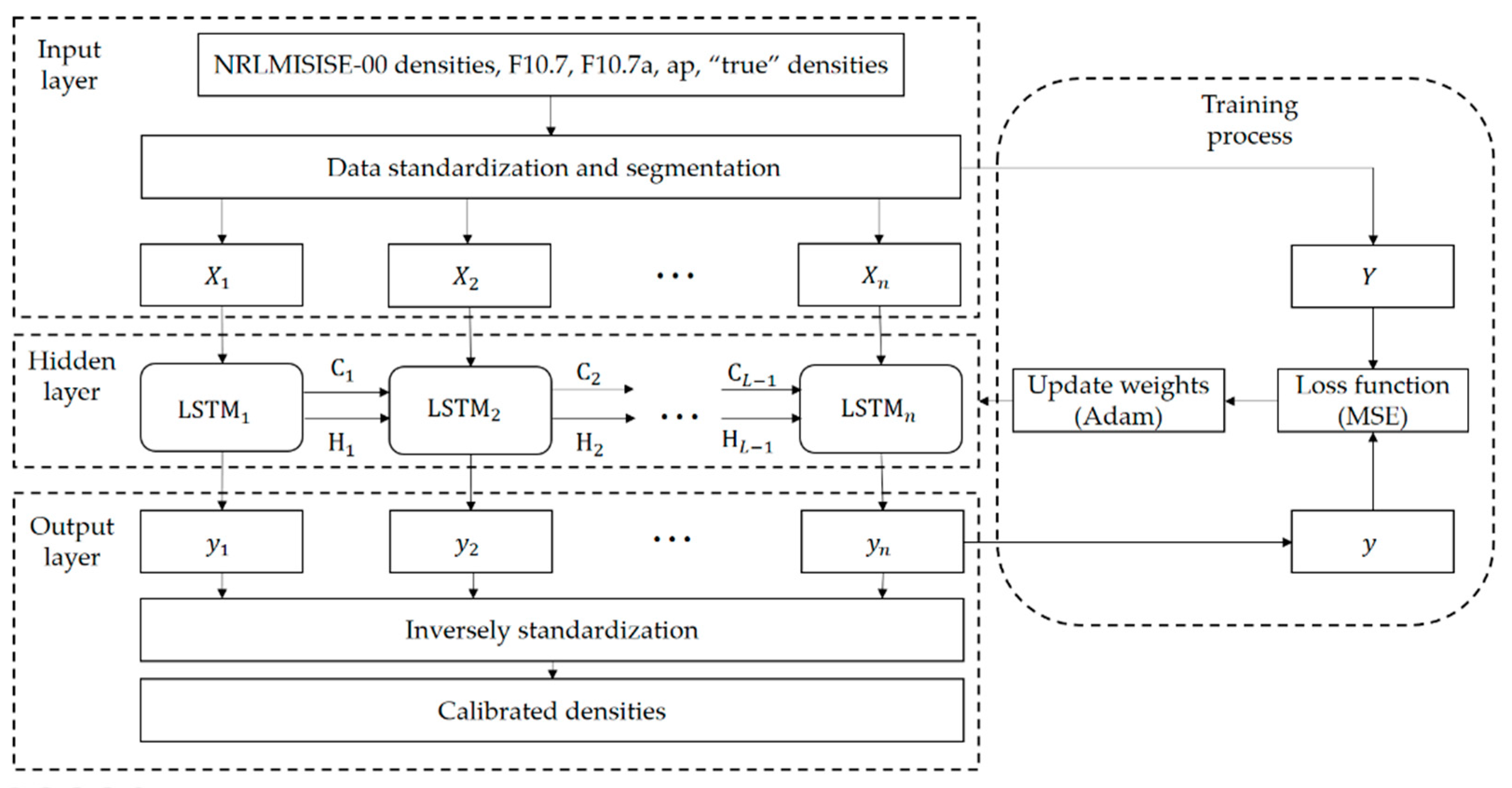
where the x o ( n ) t is a specific type of original data (empirical density, “true” density, F10.7, F10.7a or ap) at t , μ ( n ) and σ ( n ) are expectation and standard deviation of corresponding original training data, respectively. The structure of the LSTM-NRL density calibration model is shown in Figure 2, including an input layer, a hidden layer, an output layer, and the training process.
In Figure 2, the standardized data includes the sample data X and corresponding labels Y , which can be expressed as Equations (8) and (9), respectively.
X = [ X 1 X 2 X n ] = [ s 1 s 2 s t s 2 s 3 s t + 1 s n s n + 1 s t + n 1 ]
Y = [ Y 1 Y 2 Y n ] = [ ρ t ρ t + 1 ρ t + n 1 ]
where s i = ( l g ( ρ M S I S E ) i ,   F 10.7 i ,   F 10.7 a i ,   a p i ) . t is the time delay of the LSTM network, one of the important parameters, which will affect the performance of the model. For the calibration of density time series, the time delay determines how many previous data points are considered to calibrate the empirical density at the current time. The n in Equation (8) is determined by t and another parameter: sample rate. The sample rate determines how dense the density data is on the time scale. Whether small or too large, the sample rate may lead to over-fitting or under-learning of the atmospheric density features, which will affect the performance of trained model within and/or outside the training window. The accelerometer data rate is 0.1 Hz, resulting in a total of 241,920 “true” densities and sample data s i during the training period. The appropriate time delay and sample rate are found by trying different combinations. For the given problem, the time delay and the sample rate are found to be 200 data points and 60 s, respectively. More details are presented in Section 3. Therefore, the n in Equation (8) is 40,120 (n = total training data size/data sample rate-time delay = 241,920/60–200) sets of data are eventually used in the model training. The labels Y j is the “true” density at the next data point of the sample data. For example, X 1 includes 200 sample data from s 1 to s 200 , the corresponding label is l g ( ρ ) 200 .
The hidden layer of the LSTM-NRL consists of n LSTM cells, as shown in Figure 2. When X i is the input to the cell, the output y i of each cell can be represented by Equation (10).
y i = LSTM f o r w a r d ( X i , C i 1 , H i 1 )
where LSTM f o r w a r d is the LSTM forward calculation method Equations (2)–(6).
After that, the MSE is used as the loss function to calculate the difference between y and the “true” density Y . The loss function is shown in Equation (11).
MSE ( y , Y ) = 1 n i = 1 n ( y i Y i ) 2
The adaptive moment estimation (ADAM) is used to update the weights of LSTM network in the direction of the decreasing value of the loss function, as shown in Figure 2. More details about ADAM can be obtained from [39]. Lastly, X is the input to the cells in the hidden layer, whose weights are updated at last epoch, to update the weights of network for many times, then the final hidden layer and LSTM-NRL can be obtained.
When the LSTM-NRL is used to calibrate the empirical density, the output of hidden layer y i is standardized and needs to be de-standardized to obtain the calibrated density, as shown in Equation (12).
l g ( ρ ^ i ) = y i × σ + μ
where σ and μ are expectation and standard deviation of the empirical density, respectively.
In summary, the input to the LSTM-NRL include the NRLMSISE-00 empirical density, the daily F10.7, its average F10.7a in 81 days, and the 3-hourly geomagnetic index ap, and the output is the calibrated density. The input and output relationship of the LSTM-NRL model is shown in Equation (13).
l g ( ρ ^ ( t ) ) = f ( l g ( ρ M S I S E ( t ) ) , l g ( ρ M S I S E ( t ( T M S I S E 1 ) t s ) ) F 10.7 ( t ) , F 10.7 ( t ( T M S I S E 1 ) t s ) F 10.7 a ( t ) , F 10.7 a ( t ( T M S I S E 1 ) t s ) a p ( t ) , a p ( t ( T M S I S E 1 ) t s ) )
where f represents the nonlinear function of the density calibration using the LSTM-NRL, l g ( ρ ^ ( t ) ) is the calibrated density output from the LSTM-NRL at t . ρ M S I S E ( t ) , F 10.7 ( t ) , F 10.7 a ( t ) , and a p ( t ) are the empirical density, F10.7, it’s average in 81 days, and geomagnetic index at t , respectively. T M S I S E and t s are the time delay and sample rate, respectively.

2.4. Test Experiment Design

Given the training time window, from 1 January to 28 January 2007, the LSTM-NRL model is trained and its performance within and outside the training window has to be evaluated. In particular, the performance in different time spans and space weather environments after the training window is of most interest, since the LSTM-NRL model is to be used in practical applications. Eight tests are designed as follows.
  • Test 1: the purpose is to determine the time delay and sample rate. The time delay and the sample rate of the LSTM-NRL model are tuned. In the tuning, the data on 31 January 2007 is used as the test data. The parameter tuning results are presented in Section 3.1.
  • Test 2 and Test 3: the purpose is to evaluate the performance of LSTM-NRL over different time spans after the training window. Test 2 uses the data sets in a month 1–28 February 2007 as test data, and Test 3 uses the data in a year from 1 March 2007 to 29 February 2008.
  • Test 4 and Test 5: the purpose is to evaluate the performance of the LSTM-NRL model at different solar and geomagnetic activity level. Test 4 chooses 2 days, a day of high solar and geomagnetic activity on 30 January 2007 (day 30 of 2007) and a day of low solar and geomagnetic activity on 19 August 2007 (d231), as test sets to observe the performance of the LSTM-NRL model. It is noted that the 2 days in Test 4 are chosen to compare with the calibration performance of other researchers under typical high or low solar and geomagnetic activity [22,24]. To further verify the LSTM-NRL model performance during period of high or low solar and geomagnetic activity, Test 5 chooses other 3 days with high solar and geomagnetic activity (Test 5-high, day 118, 195, and 345 of 2007), and 3 days with low (Test 5-low, day 103, 204, and 322 of 2007) as test sets.
  • Test 6: the purpose is to assess the LSTM-NRL’s performance over most of CHAMP satellite’s operation life. The data in 6 full years from 2003 to 2008 is chosen as test sets, during which the orbital altitude of the satellite has changed significantly.
  • Test 7: the purpose is to demonstrate the transferring performance of the LSTM-NRL model trained using the CHAMP data. Test 7 takes the density along the orbits of two GRACE satellites as test sets.
  • Test 8: the purpose is to present the effect of the LSTM-NRL model on the orbital propagation accuracy.
The mean values of F10.7 and ap in the training process and Test 1 to Test 5 are presented in Table 1, and the trend of space weather index in the tests is shown in Figure 3. Besides, the mean values of F10.7 and ap in Test 6 are given in Section 3.4.
The blue box in Figure 2 shows the F10.7 and ap in the training process, and the yellow box and the green box present the two index values in Test 2 and Test 3, respectively.

2.5. Model Performance Evaluation

To assess the performance of the LSTM-NRL, two metrics are used: the root mean squared error (RMSE) and the Pearson correlation coefficient (R). RMSE is used to represent the deviation of the model density from the “true” density shown in Equation (14), and R measures the linear dependence between two series shown in Equation (15).
R M S E = 1 n i = 1 n ( ρ ^ i ρ i ) 2
R = i = 1 n ( ρ i ρ ¯ i ) ( ρ ^ i ρ i ^ ¯ ) i = 1 n ( ρ i ρ ¯ i ) 2 i = 1 n ( ρ ^ i ρ i ^ ¯ ) 2
where ρ is the “true” density, and ρ ^ is the density from the NRLMSISE-00 or LSTM-NRL model.
For a series of calibrated density and corresponding “true” density series, the smaller RMSE is, the closer the two density series are, and the better the calibration performance of the model is. The R between the calibrated density series and the “true” density series present the linear dependence between two series, and the R [ 0 ,   1 ] . R > 0.6 indicates a strong correlation between the two density series, and R < 0.4 indicates a weak correlation.

3. Results

3.1. Determination of the Time Delay and Sample Rate

T M S I S E and t s determine how many data sets before the current time are considered to calibrate the density, which will affect the performance of the trained model. According to Equations (8) and (10), the output of LSTM cell from the hidden layer y ( i ) is determined by X ( i ) at time i , which can be expressed by Equation (16).
X ( i ) = [ S ( i ) S ( i 1 × t s ) S ( i ( ( T M S I S E 1 ) × t s ) ]
where S ( i ) = ( l g ρ M S I S E ( i ) ,   F 10.7 ( i ) ,   F 10.7 a ( i ) ,   a p ( i ) ) . As shown in Equation (16), t s determines how dense the density data on the time scale is used to compute y ( i ) . T M S I S E determines how many data points before time i are considered to compute y ( i ) . In the training process, overly small or large t s and T M S I S E   may lead to over-fitting or under-learning of the atmospheric density features, respectively, which will affect the performance of trained model.
In this section, the appropriated time delay and the sample rate of the LSTM-NRL model are found by parameter tuning method Using the data on 31 January 2007 as the test set, Test 1 evaluates the performance of the LSTM-NRL with different T M S I S E and t s , and then the two parameters resulting in the best model performance are chosen.
Firstly, the sample rate t s is set to fixed 60 s and various T M S I S E are tried. The RMSE and R values between the calibrated density series and the “true” density series are shown in Table 2. For comparison, the two metrics between the empirical density series and the “true” density series are also presented in Table 2 too. It is noted that the best results, in terms of RMSE and R, are bold in the following tables.
As shown in Table 2, for the tried T M S I S E and t s , the LSTM-NRL performs better than the NRLMSISE-00, where the density output from the LSTM-NRL is closer to the “true” density than the empirical model. The minimum RMSE is obtained when T M S I S E is set as 200. Increasing the time delay to 300 or 500 will result in higher R, but RMSE is decreased. From this table, it is seen that the best T M S I S E is 200, corresponding to the sample rate t s = 60   s . In fact, given T M S I S E = 200 , the best sample rate t s = 60   s is obtained from the results in Table 3. Therefore, the time delay and sample rate are set to 200 and 60 s, respectively, in the following experiments.

3.2. Extrapolation Performance of the LSTM-NRL over Long Time Span

Test 2 and the Test 3 use data in one month and one year, respectively, to evaluate the long-term extrapolation performance of the LSTM-NRL outside the training window. Table 4 presents the overall performance of the LSTM-NRL during the two evaluation time spans.
As presented in Table 4, the overall RMSE values are reduced by 63.2% and 68.1% for Test 2 and Test 3, respectively, which means that the densities calibrated by LSTM-NRL during a month (Test 2) or a year (Test 3) are closer to the “true” densities than the empirical densities. The overall R values between the calibrated densities and the “true” densities are increased during the test month and test year. The calibrated densities has better linear correlation with the “true” densities than the empirical densities.
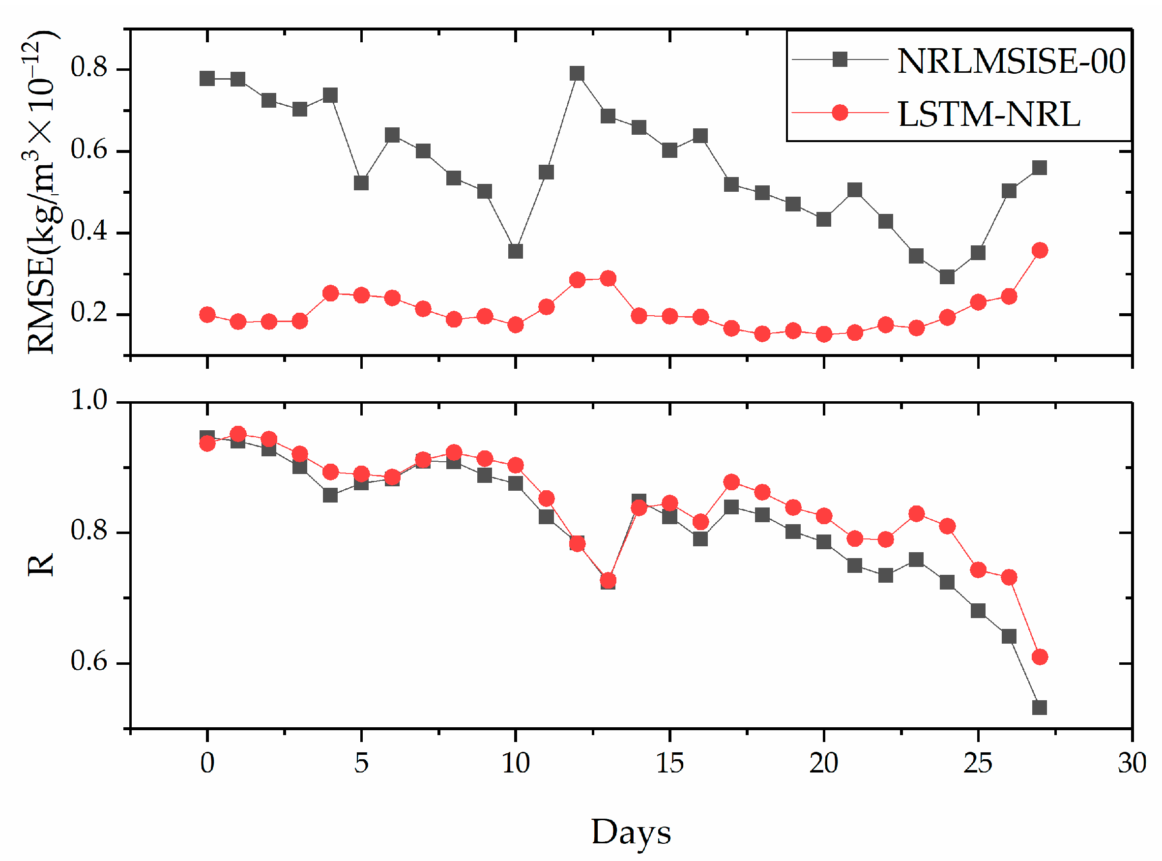
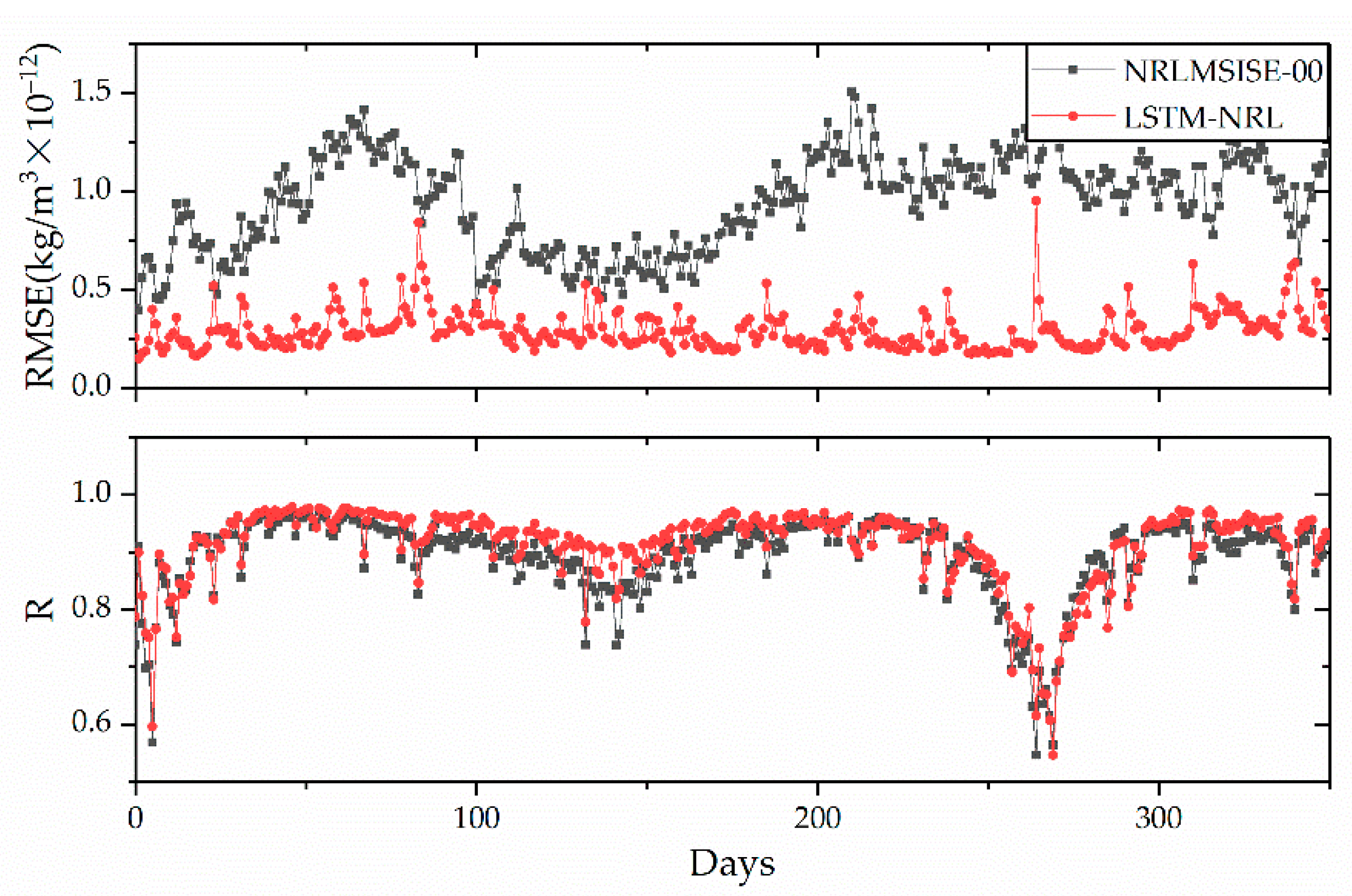
To have a more detailed knowledge about the performance of the LSTM-NRL during the test month and the test year, Figure 4 and Figure 5 show the daily RMSE and R over the time spans of Test 2 and Test 3.
As shown in Figure 4, all the RMSE values between the calibrated densities and the “true” densities in each day of the test month (Test 2) are smaller than the empirical densities. Most of the R values between the calibrated densities and the “true” densities are higher than the empirical densities. From these two metrics, the LSTM-NRL is shown to perform better than the NRLMSISE-00 model in the test month.
The daily RMSE and R values in Figure 5 show a similar picture in each day of the test year (Test 3). It is noted that, although the R values in Figure 5 has a drop after day 250, most of the R values are still greater than 0.6, which means there are strong linear correlations between the calibrated densities and the “true” densities in most days of the test year. In combination with Table 4 and Figure 4 and Figure 5, the LSTM-NRL model is still quite effectively over one year, and the density accuracy after the calibration is significantly improved.

3.3. Performance of the LSTM-NRL on Days of High and Low Solar and Geomagnetic Activity

The solar and geomagnetic activities are two major driving factors affecting the dynamics of the atmosphere. Densities computed from empirical models during the time of high solar and geomagnetic activity usually have larger errors. It would be interesting to see whether the LSTM-NRL model has better performance than the original NRLMSISE-00 model during the time of high activities, as well as the time of low activities. Test 4 and Test 5 have such days, the performance of which are presented below.
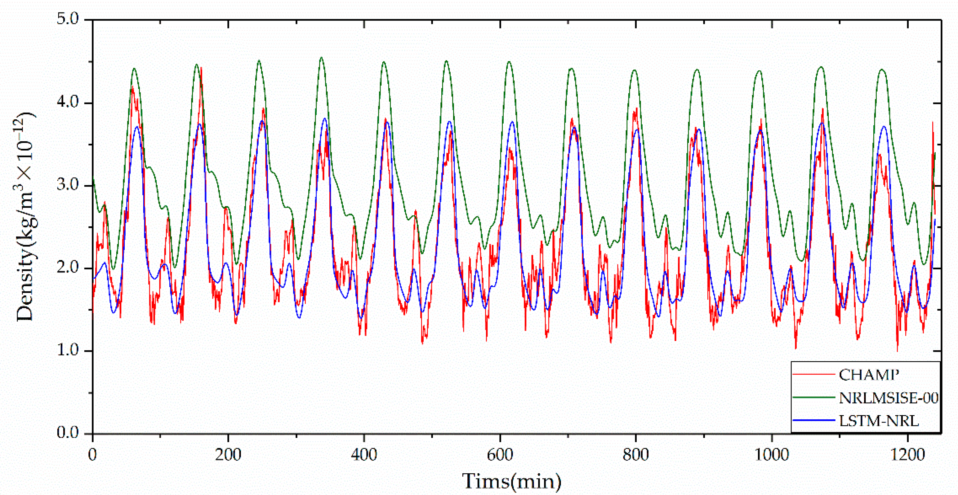
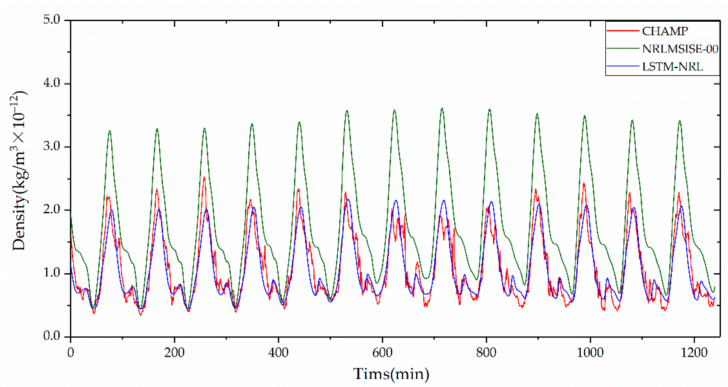
In Test 4, day 30 and day 231 of 2007 represent the times of high and low activity, respectively. The densities computed by the LSTM-NRL, the NRLMSISE-00, and the accelerometer on the two days are shown in Figure 6 and Figure 7.
It is clear that the densities from the LSTM-NRL (blue lines) are much closer to the “true” density (red lines) than those from the NRLMSISE-00 (green lines) on both days. Both in the general trends and at extremes, the densities from the LSTM-NRL are highly consistent with the “true” densities. The RMSE and R with respect to the empirical model and LSTM-NRL on the two days are presented in Table 5. The improvement on RMSE is 67.3% and 73.0% on day 30 and day 231, respectively.
As shown in Table 5, using LSTM-NRL, the RMSE between the calibrated densities and the “true” densities is reduced from 0.9128 and 0.7653 to 0.2987 and 0.2065 on the day 30 (high activity) and the day 231 (low activity), respectively. It is presented by Perez et al. [22] and Gao et al. [24] that the RMSE improvement on these two days uses different machine learning methods. The improvements by Perez et al. using RTDNN are 36.1% and 59.5% on day 30 and day 231, respectively. Following Gao et al.’s use of the Gaussian Process method, they are 43.1% and 66.4%, respectively. As a comparison, the LSTM-NRL achieves better RMSE improvements of 67.3% and 73.0%, respectively. The improvement on day 231 of low activity is more significant than that on day 30 of high activity.
On other days in Test 5, the RMSE improvements from the calibration are further confirmed, as shown in Table 6.
As shown in Table 6, the RMSE values between the calibrated densities and the “true” densities, which are shown in bold, are smaller than the no-calibrated densities, and the values of R are almost similar in all six days. On the three days of high activity, the improvements of the RMSE values by the calibration are 58.0%, 29.2%, and 62.2%, respectively. They are 77.6%, 61.2% and 81.2%, respectively, on the three days of low activity. There are strong linear correlations between the calibrated densities and the “true” densities in all six days. Again, the improvements on days of low activity are more significant than those on days of high activity.
From these results, it could be concluded that the LSTM-NRL model has a better performance in both the times of high and low solar and geomagnetic activities in 2007.

3.4. Performance of the LSTM-NRL over the CHAMP Operational Life

Test 2 and Test 3 have shown the performance improvements from the LSTM-NRL model over a month and a year after the training window of one month. In Test 6, the LSTM-NRL model is applied over the six operational years of CHAMP satellite from 2003 through 2008, and thus a more comprehensive performance evaluation is made. These six years not only cover most operational life of CHAMP, but also high solar and geomagnetic activity year (2003) and low year (2007). The yearly RMSE and R values over the six years are presented in Table 7, as well as the yearly mean F 10.7 and ap values.
As presented in Table 7, the performance of the LSTM-NRL model in terms of RMSE and R is significantly better than that of the NRLMSISE-00 model throughout the six years, although the LSTM-NRL model is trained using one month of data only. The yearly RMSE improvements are presented in Table 8. For comparison, the improvements using the RTDNN by Perez et al. are presented too. It is noted that the result of the RTDNN has the best performance without the velocity as input in the paper of Perez et al.
It can be seen that the yearly improvement of the RMSE by the LSTM-NRL is at least more than 40%, and they are 69.3% and 72.5% for 2007 and 2008, respectively. The better performance in 2007 can be attributed to the closeness between 2007 and the training window, and the similar solar and geomagnetic activity levels during these two time periods. On the other hand, Perez et al. use the data in 2003 to train RTDNN-3inputs model, and the density data in 2007 is to find the appropriate time delay. That results in better performance of the RTDNN-3inputs in 2007 and 2008, and worse performance in 2004 and 2005, which are furthest away in time from 2007. Comparing with the RTDNN-3inputs model, the LSTM-NRL not only has better performance in 2007 and 2008, but also is good in 2004 and 2005. From these analyses, it is demonstrated that the LSTM model is better suited to the problem of density calibration since the LSTM is better at memorizing and processing data over much longer periods of time.

3.5. Transferring Ability of the LSTM-NRL

An important feature of machine learning models is their transferring ability. In the case of the density calibration discussed in this paper, the data from CHAMP satellite is used to train the LSTM-NRL model. To evaluate the transferring performance of this LSTM-NLR model, experiments using data from GRACE satellites are made.
The GRACE mission consists of twin satellites (GRACE-A and GRACE-B) at the orbital altitude of 500 km and inclination of 89.96°. Both GRACE satellites are equipped with accelerometers, and thus the densities derived from the accelerometer data can be regarded as the “true” densities to evaluate the transferring ability of the LSTM-NRL model trained using the data from CHAMP which is at the altitude of 350 km and inclination of 87.18°.
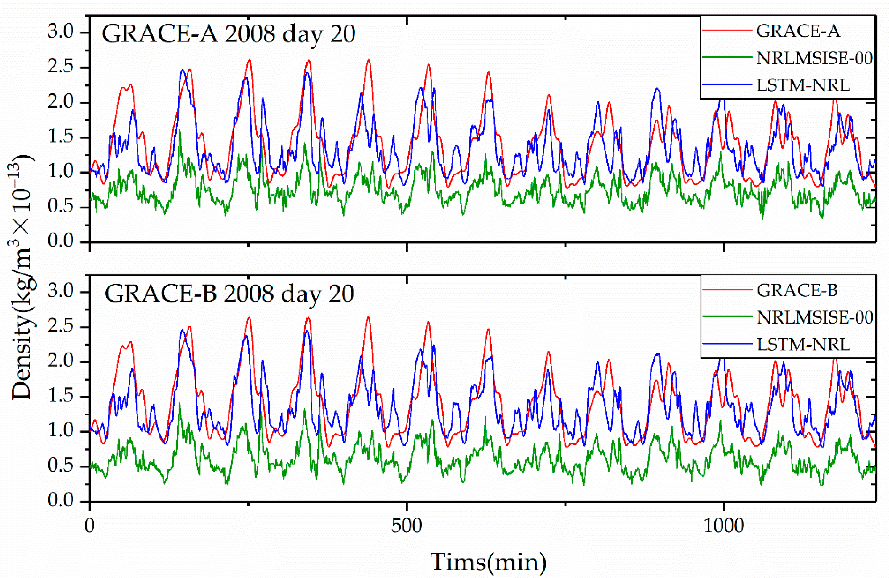
Test 7 takes the NRLMSISE-00 empirical densities, “true” densities of the two GRACE satellites, and space weather data in January 2008 as test set, to evaluate the performance of the trained LSTM-NRL model along GRACE satellite orbit. The density series along the GRACE orbits on day 10 and day 20 in January is shown in Figure 8 and Figure 9, respectively.
It can be seen that the density calibrated by the LSTM-NRL (blue lines) is closer to the “true” density (red lines) than the density computed from the NRLMSISE-00 (green lines) on the two days for both GRACE-A and GRACE-B. Both in the general trends and at extremes, the densities from the LSTM-NRL are highly consistent with the “true” densities. The LSTM-NRL shows significant calibration effect on the NRLMISISE-00 densities on two days for GRACE-A and GRACE-B. The overall performance metrics are presented in Table 9.
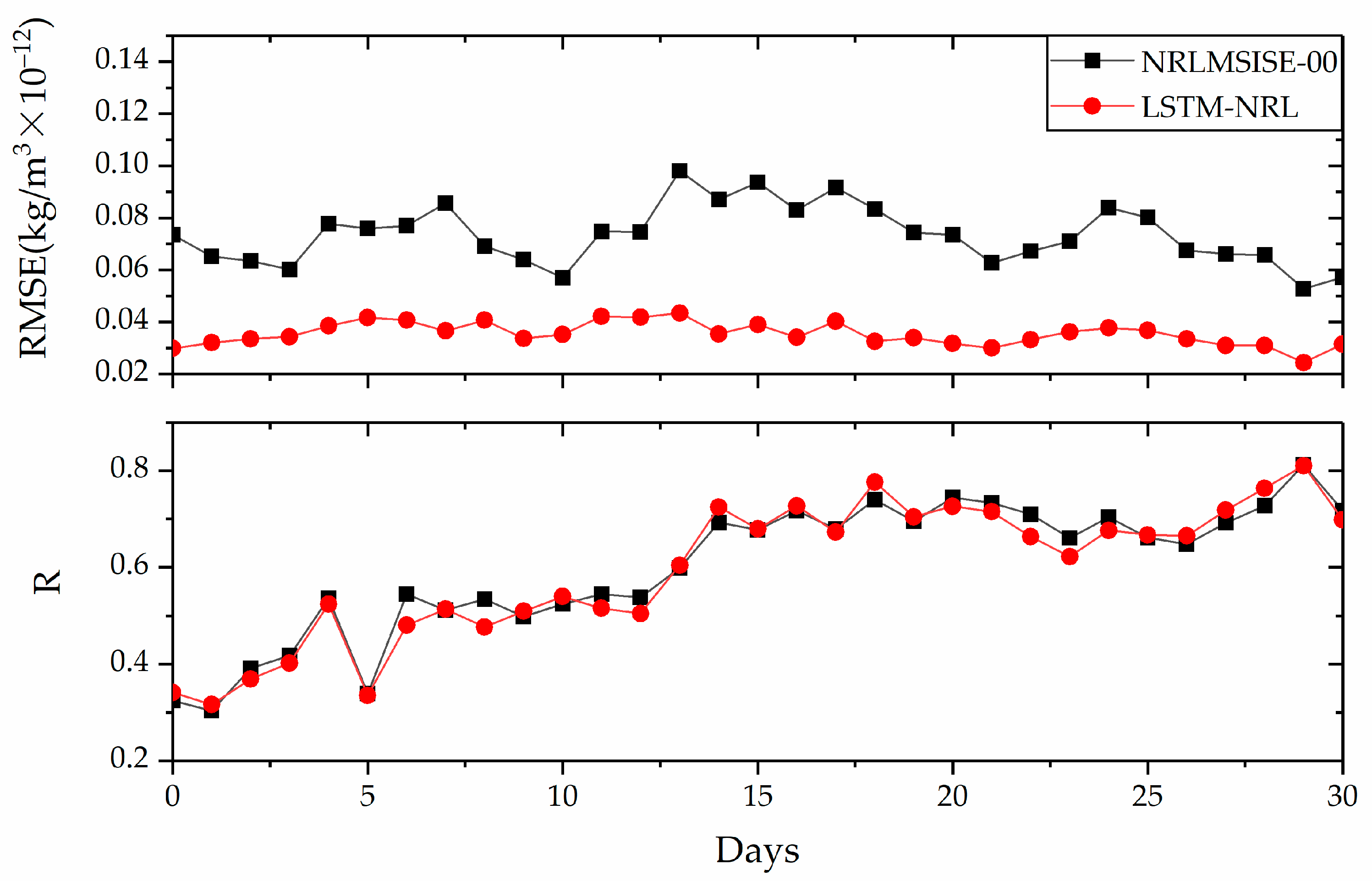
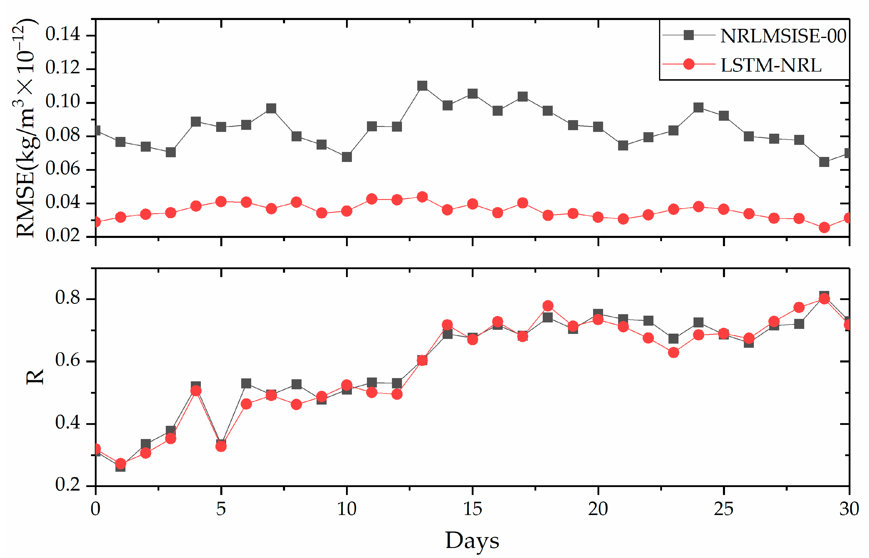
As evident from Table 9, the overall RMSE values in January 2008 are improved in January 2008 by 64.5%, 52.0%, and 58.2% for CHAMP, GRACE-A, and GRACE-B, respectively. Although the performance on CHAMP is better than the GRACE satellites, the LSTM-NRL model has shown a remarkable transferring ability when it is applied to the two GRACE satellites. This can be further demonstrated by plotting the daily RMSE and R values in Figure 10 and Figure 11.
From Figure 10, the RMSE values between the calibrated densities and the “true” densities are smaller than the NRLMSISE-00 densities for GRACE-A on each day in January 2008. The R values are mostly the same during the test month. Figure 11 shows almost the same picture of Figure 10. These two figures have clearly demonstrated the good transferring performance of the LSTM-NRL model trained using the CHAMP data, a feature important for the practical application of the model.

3.6. Applying Calibrated Density to the Orbital Propagation

A main objective of calibrating an empirical density model is to replace the empirical model with the calibrated one in order to improve orbit propagation accuracy. Test 8 is designed to demonstrate the effectiveness of the LSTM-NRL model in reducing the orbit propagation error for CHAMP satellite. The orbit prediction errors are computed as the difference between the predicted positions and the positions computed using GPS-derived precise ephemeris. In this test, three density series are used in the CHAMP orbit determination and prediction: the density calibrated by the LSTM-NRL, the density computed from the NRLMISIE-00 model, and the “true” density derived from the CHAMP accelerometer data. For each density series, the orbit determination is first performed using the precise positions over one day on 1 April 2007, in which the position and velocity vectors as well as the drag coefficient C d are estimated, and the orbit is then predicted for 7 days from April 2 to April 8. Figure 12 shows the three series of prediction errors in along the track direction, since the density error is dominantly affecting the orbit in along the track direction.
As shown in Figure 12, the orbit prediction errors using any of the three density series in the first four days are at the similar level. However, in the final three days, the advantage of using the calibrated density becomes clear. At the end of seven days, the error using the NRLMSISE-00 model is 12.2 km, which is significantly larger than the error of 6.7 km using the calibrated density. It is noted that the error at the end of seven days using the “true” density is 4.9 km, the smallest among the three error values. This example shows that the LSTM-NRL model is effective in reducing the orbit determination and prediction errors.

4. Discussion

This paper has proposed to apply the LSTM neural network to calibrate empirical atmospheric density models, and the NRLMSISE-00 model is calibrated using the density derived from CHAMP accelerometer data, resulting in the LSTM-NRL model. The calibration performance is comprehensively evaluated with RMSE and the Pearson coefficient R as the metrics and the density derived from the accelerometer data as “truth”. The evaluation of the LSTM-NRL performance includes the following parts.
First of all, the effects of different combinations of two critical parameters, the time delay and sample rate on the performance of the LSTM-NRL, are presented in Section 3.1. The training of the LSTM-NRL model uses the data in four weeks from 1 January 2007 to 28 January 2007. The two parameters are tuned using the data on 31 January 2007 (Test 1). The appropriate values for the two parameters are found to be 200 and 60 s, respectively.
Secondary, the extrapolation performance of the trained model is evaluated over a long time span. Test 2 and Test 3 take data over one month and one year as test sets, respectively; the results show that the RMSEs of the calibrated density series are reduced by 63.2% and 68.1% for Test 2 and Test 3, respectively, comparing with those of the density series computed from the NRLMSISE-00 model. Extending the testing time span to six years from 2003 through 2008 (Test 6), the calibrated model outperforms the NRLMSISE-00 model in terms of the RMSE by a significant margin, with at least a 40% reduction in yearly RMSE. Although the LSTM-NRL model is trained using one month of data only, the performance of the LSTM-NRL model in terms of RMSE and R is significantly better than that of the NRLMSISE-00 model throughout the six years. The yearly improvement of the RMSE by the LSTM-NRL is at least more than 40%; they are 69.3% and 72.5% for 2007 and 2008, respectively. The better performance in 2007 can be attributed to the closeness between 2007 and the training window, and the similar solar and geomagnetic activity levels during these two time periods.
Then, the performance of the calibrated model in different space weather environment is also evaluated in Test 4 and Test 5, where eight days in 2007 of high or low solar and geomagnetic activity are chosen in total. The calibrated densities on all these days are much closer to the “true” densities than those from the NRLMSISE-00 model. It is also found that the calibration has better performance on the days of low activity.
Moreover, Test 7 is designed to study the transferring performance of the LSTM-NRL model trained by the CHAMP data, when the model is applied along the orbits of two GRACE satellites. Using the densities derived from GRACE accelerometer data in January 2008 as a reference, the LSTM-NRL is shown to have significantly better performance in terms of the RMSE than the NRLMSISE-00 model. The overall RMSE reduction for GRACE-A and GRACE-B is 52.0% and 58.2%, respectively; a clear indication that the LSTM-NRL model has remarkable transferring ability.
Besides, the LSTM-NRL model is also tested to examine its effectiveness in reducing the orbit prediction errors in Test 8. It is found that, over a 7-day prediction time, the orbit errors using the calibrated, “true” and NRLMSISE-00 density, respectively, are at similar level in the first four days. Nevertheless, at the end of the seven days, the error is 12.2 km using the NRLMSISE-00 model, and is reduced to 6.7 km when the LSTM-NRL model is used.

5. Conclusions

The empirical atmospheric mass density model error remains a dominant error source for accurate orbit determination and prediction for LEO satellites. An effective approach to reduce the model errors is to calibrate the empirical models using satellite tracking data and mass densities derived from accelerometer data. The evaluation results of the LSTM-NRL performance show that the calibration model not only works over different time spans, but is also suitable on days of different space weather environment. More than that, the transferring ability and the ability of improving orbit propagation accuracy of the LSTM-NRL are illustrated.
In summary, the paper has demonstrated that the LSTM neural network is able to effectively calibrate the NRLMSISE-00 model, given the accurate and dense densities derived from the spaceborne accelerometer data. In the next phase of the research, the developed approach will be applied to calibrate other empirical models using not only the density from the accelerometer data but also the density derived from precise orbit positions.

Author Contributions

Conceptualization, J.S.; Data curation, Y.Z. and J.Y.; Formal analysis, J.Y. and J.S.; Funding acquisition, J.S.; Investigation, Y.Z., J.Y. and J.C.; Methodology, Y.Z., J.Y., J.C. and J.S.; Resources, J.S.; Software, Y.Z. and J.Y.; Supervision, J.S.; Validation, Y.Z.; Visualization, Y.Z.; Writing—original draft, Y.Z.; Writing—review & editing, J.S. All authors have read and agreed to the published version of the manuscript.

Funding

This work is supported in part by the National Natural Science Foundation of China under Grant 41874036.

Institutional Review Board Statement

Not applicable.

Informed Consent Statement

Not applicable.

Data Availability Statement

Data is contained within this article.

Conflicts of Interest

The authors declare that they have no conflict of interest to report regarding the present study.

References

  1. Montenbruck, O.; Gill, E.; Lutze, F. Satellite orbits: Models, methods, and applications. Appl. Mech. Rev. 2002, 55, B27–B28. [Google Scholar] [CrossRef]
  2. Prieto, D.M.; Graziano, B.P.; Roberts, P.C.E. Spacecraft drag modelling. Prog. Aerosp. Sci. 2014, 64, 56–65. [Google Scholar] [CrossRef] [Green Version]
  3. Qian, L.; Burns, A.G.; Emery, B.A.; Foster, B.; Lu, G.; Maute, A.; Richmond, A.D.; Roble, R.G.; Solomon, S.C.; Wang, W. The NCAR TIE-GCM: A community model of the coupled thermosphere/ionosphere system. Model. Ionos. Thermosphere Syst. 2014, 201, 73–83. [Google Scholar]
  4. Richmond, A.D.; Ridley, E.C.; Roble, R.G. A Thermosphere/ionosphere general-circulation model with coupled electrodynamics. Geophys. Res. Lett. 1992, 19, 601–604. [Google Scholar] [CrossRef]
  5. Ridley, A.; Deng, Y.; Toth, G. The global ionosphere—Thermosphere model. J. Atmos. Sol. Terr. Phys. 2006, 68, 839–864. [Google Scholar] [CrossRef]
  6. Emmert, J.T. Thermospheric mass density: A review. Adv. Space Res. 2015, 56, 773–824. [Google Scholar] [CrossRef]
  7. Chen, J.; Sang, J. Thermospheric mass density measurement from precise orbit ephemeris. Geod. Geodyn. 2016, 7, 210–215. [Google Scholar] [CrossRef] [Green Version]
  8. Deng, Y.; Ridley, A.J. Possible reasons for underestimating Joule heating in global models: E field variability, spatial resolution, and vertical velocity. J. Geophys. Res. Space Phys. 2007, 112. [Google Scholar] [CrossRef] [Green Version]
  9. Picone, J.M.; Hedin, A.E.; Drob, D.P.; Aikin, A.C. NRLMSISE-00 empirical model of the atmosphere: Statistical comparisons and scientific issues. J. Geophys. Res. Space Phys. 2002, 107, 1468–1483. [Google Scholar] [CrossRef]
  10. Bowman, B.; Tobiska, W.K.; Marcos, F.; Huang, C.; Lin, C.; Burke, W. A new empirical thermospheric density model JB2008 using new solar and geomagnetic indices. In Proceedings of the AIAA/AAS Astrodynamics Specialist Conference and Exhibit, Honolulu, HI, USA, 18–21 August 2008. [Google Scholar]
  11. Bruinsma, S. The DTM-2013 thermosphere model. J. Space Weather Space Clim. 2015, 5, A1. [Google Scholar] [CrossRef] [Green Version]
  12. Marcos, F.A.; Kendra, M.J.; Griffin, J.M.; Bass, J.N.; Larson, D.R.; Liu, J.J. Precision low earth orbit determination using atmospheric density calibration. J. Astronaut. Sci. 1998, 46, 395–409. [Google Scholar] [CrossRef]
  13. Nazarenko, A.I.; Cefola, P.J.; Yurasov, V. Advances in the Astronautical Sciences. In Spaceflight Mechanics; Amer Astronautical Society: Springfield, VA, USA, 1998; Volume 99, pp. 1–2. [Google Scholar]
  14. Shi, C.; Li, W.; Li, M.; Zhao, Q.; Sang, J. Calibrating the scale of the NRLMSISE00 model during solar maximum using the two line elements dataset. Adv. Space Res. 2015, 56, 1–9. [Google Scholar] [CrossRef]
  15. Storz, M.F.; Bowman, B.R.; Branson, M.J.I.; Casali, S.J.; Tobiska, W.K. High accuracy satellite drag model (HASDM). Space Weather 2005, 36, 2497–2505. [Google Scholar]
  16. Bowman, B.; Storz, M. Time series analysis of HASDM thermospheric temperature and density corrections. In Proceedings of the AIAA/AAS Astrodynamics Specialist Conference and Exhibit, Monterey, CA, USA, 5–8 August 2002. [Google Scholar]
  17. Emmert, J.T.; Picone, J.M.; Lean, J.L.; Knowles, S.H. Global change in the thermosphere: Compelling evidence of a secular decrease in density. J. Geophys. Res. Space Phys. 2004, 109. [Google Scholar] [CrossRef]
  18. Picone, J.M.; Emmert, J.T.; Lean, J.L. Thermospheric densities derived from spacecraft orbits: Accurate processing of two-line element sets. J. Geophys. Res. Space Phys. 2005, 110, 110. [Google Scholar] [CrossRef]
  19. Cefola, P.J.; Proulx, R.J.; Nazarenko, A.I.; Yurasov, V.S. Advances in the Astronautical Sciences. In Astrodynamics; Univelt: Escondido, CA, USA, 2003; pp. 1–3. [Google Scholar]
  20. Doornbos, E.; Klinkrad, H.; Visser, P. Use of two-line element data for thermosphere neutral density model calibration. Adv. Space Res. 2008, 41, 1115–1122. [Google Scholar] [CrossRef]
  21. Sang, J.; Smith, C.; Zhang, K. Towards accurate atmospheric mass density determination Using precise positional information of space objects. Adv. Space Res. 2012, 49, 1088–1096. [Google Scholar] [CrossRef]
  22. Perez, D.; Bevilacqua, R. Neural Network based calibration of atmospheric density models. Acta Astronaut. 2015, 110, 58–76. [Google Scholar] [CrossRef]
  23. Perez, D.; Wohlberg, B.; Lovell, T.A.; Shoemaker, M.; Bevilacqua, R. Orbit-centered atmospheric density prediction using artificial neural networks. Acta Astronaut. 2014, 98, 9–23. [Google Scholar] [CrossRef]
  24. Gao, T.; Peng, H.; Bai, X. Calibration of atmospheric density model based on Gaussian Processes. Acta Astronaut. 2020, 168, 273–281. [Google Scholar] [CrossRef]
  25. Chen, H.; Liu, H.; Hanada, T. Storm-time atmospheric density modeling using neural networks and its application in orbit propagation. Adv. Space Res. 2014, 53, 558–567. [Google Scholar] [CrossRef]
  26. Mehta, P.M.; Walker, A.; Lawrence, E.; Linares, R.; Higdon, D.; Koller, J. Modeling satellite drag coefficients with response surfaces. Adv. Space Res. 2014, 54, 1590–1607. [Google Scholar] [CrossRef]
  27. Mehta, P.M.; Walker, A.C.; Sutton, E.K.; Godinez, H.C. New density estimates derived using accelerometers on board the CHAMP and GRACE satellites. Space Weather-the International. J. Res. Appl. 2017, 15, 558–576. [Google Scholar]
  28. Walker, A.; Mehta, P.; Koller, J. Drag Coefficient Model Using the Cercignani-Lampis-Lord Gas-Surface Interaction Model. J. Spacecr. Rockets 2014, 51, 1544–1563. [Google Scholar] [CrossRef]
  29. Sutton, E.K. Effects of Solar Disturbances on the Thermosphere Densities and Winds from CHAMP and GRACE Satellite Accelerometer Data. Ph.D. Thesis, University of Colorado, Boulder, CO, USA, 2008. [Google Scholar]
  30. GFZ Data Services. Available online: https://dataservices.gfz-potsdam.de/portal/?q=champ* (accessed on 1 May 2021).
  31. Werbos, P.J. Backpropagation through Time—What it does and how to do it. Proc. IEEE 1990, 78, 1550–1560. [Google Scholar] [CrossRef] [Green Version]
  32. Williams, R.J.; Zipser, D. Gradient-based learning algorithms for recurrent. In Backpropagation: Theory, Architectures, and Applications; L. Erlbaum: Hillsdale, NJ, USA, 1995; p. 433. [Google Scholar]
  33. Hochreiter, S. The vanishing gradient problem during learning recurrent neural nets and problem solutions. Int. J. Uncertain. Fuzziness Knowl. Based Syst. 1998, 6, 107–116. [Google Scholar] [CrossRef] [Green Version]
  34. Hochreiter, S.; Schmidhuber, J. Long short-term memory. Neural Comput. 1997, 9, 1735–1780. [Google Scholar] [CrossRef] [PubMed]
  35. Tapping, K.F. The 10.7 cm solar radio flux (F10.7). Space Weather 2013, 11, 394–406. [Google Scholar] [CrossRef]
  36. Knipp, D.J.; Tobiska, W.K.; Emery, B.A. Direct and indirect thermospheric heating sources for solar cycles 21–23. Sol. Phys. 2004, 224, 495–505. [Google Scholar] [CrossRef]
  37. Bartels, J. The geomagnetic measures for the time-variations of solar corpuscular radiation, described for use in correlation studies in other geophysical fields. Ann. Intern. Geophys. 1957, 4, 227–236. [Google Scholar]
  38. EOP and Space Weather Data. Available online: https://celestrak.com/SpaceData/ (accessed on 1 May 2021).
  39. Kingma, D.P.; Ba, J.L. Adam: A method for Stochastic Optimization. In Proceedings of the 3rd International Conference for Learning Representations, San Diego, CA, USA, 7–9 May 2015. [Google Scholar]
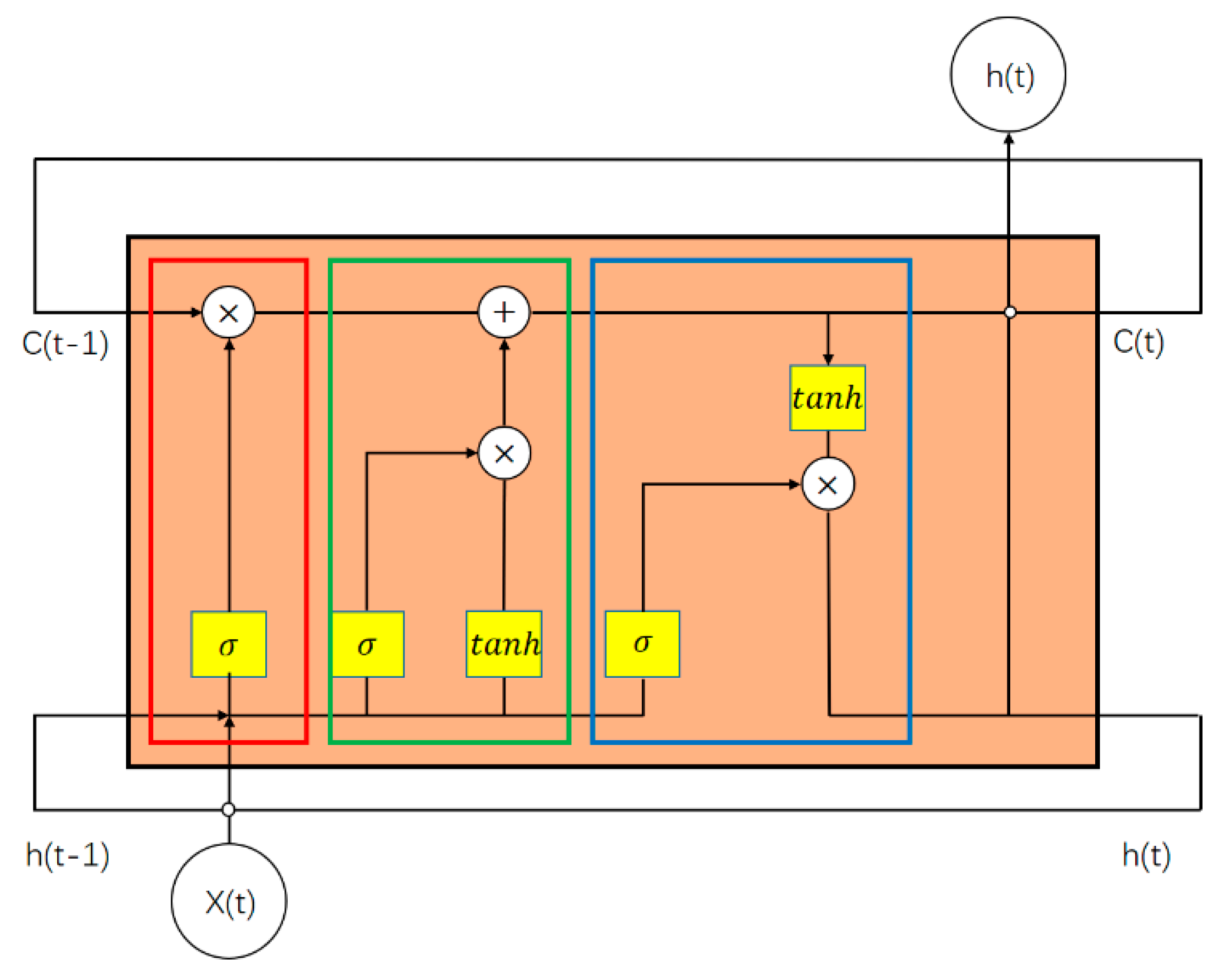
Figure 1. The structure of a LSTM cell.
Atmosphere 12 00925 g001
Figure 2. The structure of the LSTM-NRL calibration model.
Atmosphere 12 00925 g002
Figure 3. The trend of F10.7 and ap in 5 Tests.
Atmosphere 12 00925 g003
Figure 4. The daily RMSE and R over a month of Test 2.
Atmosphere 12 00925 g004
Figure 5. The daily RMSE and R over a year of Test 3.
Atmosphere 12 00925 g005
Figure 6. The three density series on day 30 of 2007, Test 4.
Atmosphere 12 00925 g006
Figure 7. The three density series on day 231 of 2007, Test 4.
Atmosphere 12 00925 g007
Figure 8. The density series along the GRACE orbits on day 10 of 2008.
Atmosphere 12 00925 g008
Figure 9. The density series along the GRACE orbits on day 20 of 2008.
Atmosphere 12 00925 g009
Figure 10. The daily RMSE and R values in January 2018, GRACE-A.
Atmosphere 12 00925 g010
Figure 11. The daily RMSE and R values in January 2018, GRACE-B.
Atmosphere 12 00925 g011
Figure 12. The CHAMP orbit prediction errors in the along track direction in 7 days.
Atmosphere 12 00925 g012
Table 1. The mean of solar radio flux (F10.7) and geomagnetic index (ap) in different time span.
TexstTime SpanMean of F10.7 (sfu)Mean of ap (nT)
Train1 January 2007–28 January 200780.348.43
Test 131 January 200786.9419.46
Test 21 February 2007–28 February 200775.87.08
Test 31 March 2007–29 February 200871.647.61
Test 4-d3030 January 200784.924
Test 4-d23119 August 200769.44
Test 5-high28 April 2007 & 14 July 2007 & 11 December 200786.0 & 78.2 & 90.528.0 & 19.0 & 16.0
Test 5-low13 April 2007 & 23 July 2007 & 18 November 200768.0 & 69.3 & 67.21.0 & 3.0 & 2.0
Table 2. The performance of the LSTM-NRL when changing T M S I S E . It is noted that the best results, in terms of RMSE and R, are bold in the table.
Model T M S I S E t s ( s ) R M S E ( kg m 3 × 10 12 ) R
NRLMSISE-00--1.04870.8761
LSTM-NRL10600.28990.9000
20600.27420.9093
50600.28220.9093
100600.27150.9105
200600.26160.9152
300600.26460.9157
500600.30530.9273
Table 3. The performance of the LSTM-NRL when changing the t s . It is noted that the best results, in terms of RMSE and R, are bold in the table.
Model T M S I S E t s ( s ) R M S E ( kg m 3 × 10 12 ) R
NRLMSISE-00--1.04870.8761
LSTM-NRL200300.30140.9057
200600.26160.9152
2001200.26670.9163
2001800.31810.9137
2003000.36320.8775
2006000.36020.8720
Table 4. The overall performance of the LSTM-NRL in Test 2 and Test 3. It is noted that the best results, in terms of RMSE and R, are bold in the table.
Model Time SpanTest 2Test 3
LSTM-NRLR1 month0.88590.9283
RMSE ( kg m 3 × 10 12 )0.21150.3129
NRLMSISE-00R1 year0.85690.9055
RMSE ( kg m 3 × 10 12 )0.57470.9799
Table 5. The performance of the LSTM-NRL in Test 4. It is noted that the best results, in terms of RMSE and R, are bold in the table.
DayModelRMSE
( kg m 3 × 10 12 )
RImprovement on RMSE
Test4-d30
( F 10.7 = 84.9 s f u , A p = 24 n T )
NRLMSISE-000.91280.8643-
LSTM-NRL0.29870.918467.3%
Test4-d231
( F 10.7 = 69.4 s f u , A p = 4 n T )
NRLMSISE-000.76530.9230-
LSTM-NRL0.20650.944073.0%
Table 6. The performance of the LSTM-NRL in Test 5. It is noted that the best results, in terms of RMSE and R, are bold in the table.
DayModelRMSE ( kg m 3 × 10 12 ) R
Test5-high2007d118LSTM-NRL0.51140.9403
NRLMSISE-001.21770.9270
2007d195LSTM-NRL0.49080.8672
NRLMSISE-000.69370.8302
2007d345LSTM-NRL0.40290.7684
NRLMSISE-001.06590.8146
Test5-low2007d103LSTM-NRL0.21220.9692
NRLMSISE-000.94790.9657
2007d204LSTM-NRL0.23220.8975
NRLMSISE-000.59890.8303
2007d322LSTM-NRL0.19960.8032
NRLMSISE-001.05960.7489
Table 7. The performance of the LSTM-NRL in 6 years from 2013 through 2018. It is noted that the best results, in terms of RMSE and R, are bold in the table.
YearModelRMSE ( kg m 3 × 10 12 ) R
2003
( F 10.7 = 139.4 s f u , A p = 12.5 n T )
NRLMSISE-000.96590.8668
LSTM-NRL0.43930.9398
2004
( F 10.7 = 106.5 s f u , A p = 13.4 n T )
NRLMSISE-000.68820.9075
LSTM-NRL0.38860.9435
2005
( F 10.7 = 91.72 s f u , A p = 13.5 n T )
NRLMSISE-000.76960.8902
LSTM-NRL0.45750.9244
2006
( F 10.7 = 80.0 s f u , A p = 8.5 n T )
NRLMSISE-000.77050.9068
LSTM-NRL0.31840.9346
2007
( F 10.7 = 73.1 s f u , A p = 7.5 n T
NRLMSISE-000.92770.9025
LSTM-NRL0.28440.9331
2008
( F 10.7 = 68.6 s f u , A p = 6.9 n T )
NRLMSISE-001.31100.8988
LSTM-NRL0.36110.9335
2003~2008
( F 10.7 = 91.4 s f u , A p = 11.9 n T )
NRLMSISE-000.92970.8721
LSTM-NRL0.37910.9411
2004~2008
( F 10.7 = 84.0 s f u , A p = 9.5 n T )
NRLMSISE-000.92210.8761
LSTM-NRL0.36540.9395
Table 8. The RMSE improvement comparison between LSTM-NRL and RTDNN-3inputs in 6 years.
YearYearly RMSE Improvement
LSTM-NRLPerez (RTDNN-3inputs) 1
200354.5%-
200443.1%14.7%
200540.5%5.9%
200658.7%28.6%
200769.3%47.2%
200872.5%45.0%
2004–200860.4%32.6%
1 3 inputs include the density estimated by the DEM-2013, JB2008 and NRLMSISE-00.
Table 9. The RMSE and R of the density series along the orbits of three satellites in January 2008. It is noted that the best results, in terms of RMSE and R, are bold in the table.
SatelliteModelRMSE   ( kg m 3 × 10 12 ) R
CHAMPNRLMSISE-001.06460.9269
LSTM-NRL0.37830.9479
GRACE-ANRLMSISE-000.07430.7256
LSTM-NRL0.03570.7562
GRACE-BNRLMSISE-000.08570.7231
LSTM-NRL0.03580.7552
Publisher’s Note: MDPI stays neutral with regard to jurisdictional claims in published maps and institutional affiliations.