Article

Urban-Induced Changes on Local Circulation in Complex Terrain: Central Mexico Basin

by
Lourdes P. Aquino-Martínez
1,
Arturo I. Quintanar
2,*,
Carlos A. Ochoa-Moya
2,
Erika Danaé López-Espinoza
2,
David K. Adams
2 and
Aron Jazcilevich-Diamant
2
1
Posgrado en Ciencias de la Tierra, UNAM, Mexico City 04510, Mexico
2
Centro de Ciencias de la Atmósfera, UNAM, Mexico City 04510, Mexico
*
Author to whom correspondence should be addressed.
Atmosphere 2021, 12(7), 904; https://doi.org/10.3390/atmos12070904
Submission received: 5 June 2021 / Revised: 25 June 2021 / Accepted: 9 July 2021 / Published: 14 July 2021
(This article belongs to the Special Issue Coastal and Urban Meteorology)

Abstract

:
Land use land cover (LULC) significantly impacts local circulation in the Mexico Basin, particularly wind field circulations such as gap winds, convergence lines, and thermally induced upslope/downslope wind. A case study with a high-pressure system over the Mexico Basin isolates the influence of large-scale synoptic forcing. Numerical simulations reveal a wind system composed of meridional circulation and a zonal component. Thermal pressure gradients between the Mexico basin and its colder surroundings create near-surface convergence lines as part of the meridional circulation. Experiments show that the intensity and organization of meridional circulations and downslope winds increase when LULC changes from natural and cultivated land to urban. Zonal circulation exhibits a typical circulation pattern with the upslope flow and descending motion in the middle of the basin. Large values of moist static energy are near the surface where air parcels pick up energy from the surface either as fluxes of enthalpy or latent heat. Surface heat fluxes and stored energy in the ground are drivers of local circulation, which is more evident in zonal circulation patterns.

1. Introduction

The interaction of local orographic circulations with urbanization effects is the focus of many past and recent observational, theoretical, and modeling studies ([1,2,3,4]). Urban and built-up areas continue to proliferate around the world, with many cities and industrial complexes built within complex terrain and valleys [5]. Compounding this problem, a combination of synoptic conditions, climate change, and deteriorated air quality conditions aggravate citizen’s health conditions in large urban centers [6]. The conversion of extensive land use areas, from natural to urban, implies significant changes in the thermodynamic, moisture, planetary boundary layer structure (PBL), and surface energy budget fields [7]. By replacing a natural surface cover with an impervious surface, the overlying air temperature of the urban area increases relative to its natural and rural surroundings due to larger sensible heat fluxes (SHF). This phenomenon, known as Urban Heat Island (UHI), is more intense when light winds and clear skies are present. In Bornstein ([8,9]), the author was a pioneer in the study of this phenomenon in New York City. Oke [10] presented an extensive review of observational studies of the characteristics, causes, and effects of the UHI. Significant advances have been made in recent decades on the subject, particularly on the relation between synoptic conditions and the UHI development. For example in Central Europe [11], have looked at how different anticyclonic patterns influence the magnitude of the UHI while [12], and [13] find that even under disturbed anticyclonic conditions with significant cloudiness and wind the UHI can still be detected in the diurnal cycle.
Jauregui [14] and Jauregui [15] first documented the diurnal evolution of the UHI in the Mexico Basin, which is home to one of the largest megacities globally, with more than 22 million inhabitants. The consequent urban growth has promoted an extraordinary change in land cover (LULC) in the basin, especially on the piedmont and slopes of mountains generating changes in atmospheric thermodynamics whose immediate effect is the generation of very intense UHI effects. More recently, with surface data from urban and rural stations Cui and De Foy [16] finds that the most intense UHI occurs in the dry period (winter and part of spring), reaching temperature differences between urban and rural areas of about 5 °C. The UHI also gives rise to vertical motion over urban areas, which in turn produces low-level wind convergence ([17,18,19]). This local circulation interacts with a diurnal wind system consisting of upslope and downslope winds at the Mexico Basin’s mountain slopes. Solar radiation produces diurnal temperature and density changes over the mountain slopes in the morning (upslope) and radiative cooling (downslope) later at night and early morning, respectively [20]. Klaus et al. [17] discuss how Mexico Basin’s UHI intensity increases during the night and early morning by downslope winds from the surrounding mountains increasing low-level convergence at or near the urban area. More recently, Ganbat et al. [2] perform two-dimensional idealized numerical experiments with a mountain and an urban area to study the interactions between the mountain upslope/downslope winds with those that the UHI generates. They find that the UHI circulation can counteract the morning upslope winds while enhancing the downslope winds later in the evening. Klaus et al. [17] find similar results from observations for the Mexico Basin during a dry period (January–February, 1995) with upper-level weak anticyclonic synoptic forcing. In addition to this orographic wind system, past studies for the Mexico Basin have uncovered and analyzed the existence of a low-level diurnal southerly jet southeast of the Mexico Basin, denoted hereafter as the Chalco jet. Usually, the Chalco jet climbs the southeastern pass from Morelos Basin (Chalco pass) and then meets a northeasterly wind amid the Mexico Basin during the day and sometimes reverses direction at night. The intensity and impact of the Chalco jet in the low-level circulation of the basin generate lines of strong wind convergence that move northeastward north of the Mexico Basin ([19,21,22,23]). The origin of the Chalco jet lies within the thermally induced pressure gradients from the colder air surrounding the warmer elevated Mexico Basin (see discussions by [20,23,24]). Previous studies have revealed some aspects of the diurnal three-dimensional wind system of the Mexico Basin. However, it is still an open question on how LULC impacts local circulation and near-surface wind field circulations such as gap winds, convergence lines, and thermally induced upslope/downslope wind at the foot of mountain chains. In this paper, we combine observations and WRF model to focus on the diurnal evolution of the UHI and the wind systems generated by topography under conditions of a high-pressure system over the region. Section 2 presents the materials and methods used to define optimal days where weak synoptic forcing is present with an enhanced UHI. Section 3 presents the diurnal cycle characteristics of the Mexico Basin, the control experiment validation, and the hypothesis testing experiments needed to isolate the effect of the UHI from the entire wind system. Finally, Section 4 contains a summary and conclusions.

2. Materials and Methods

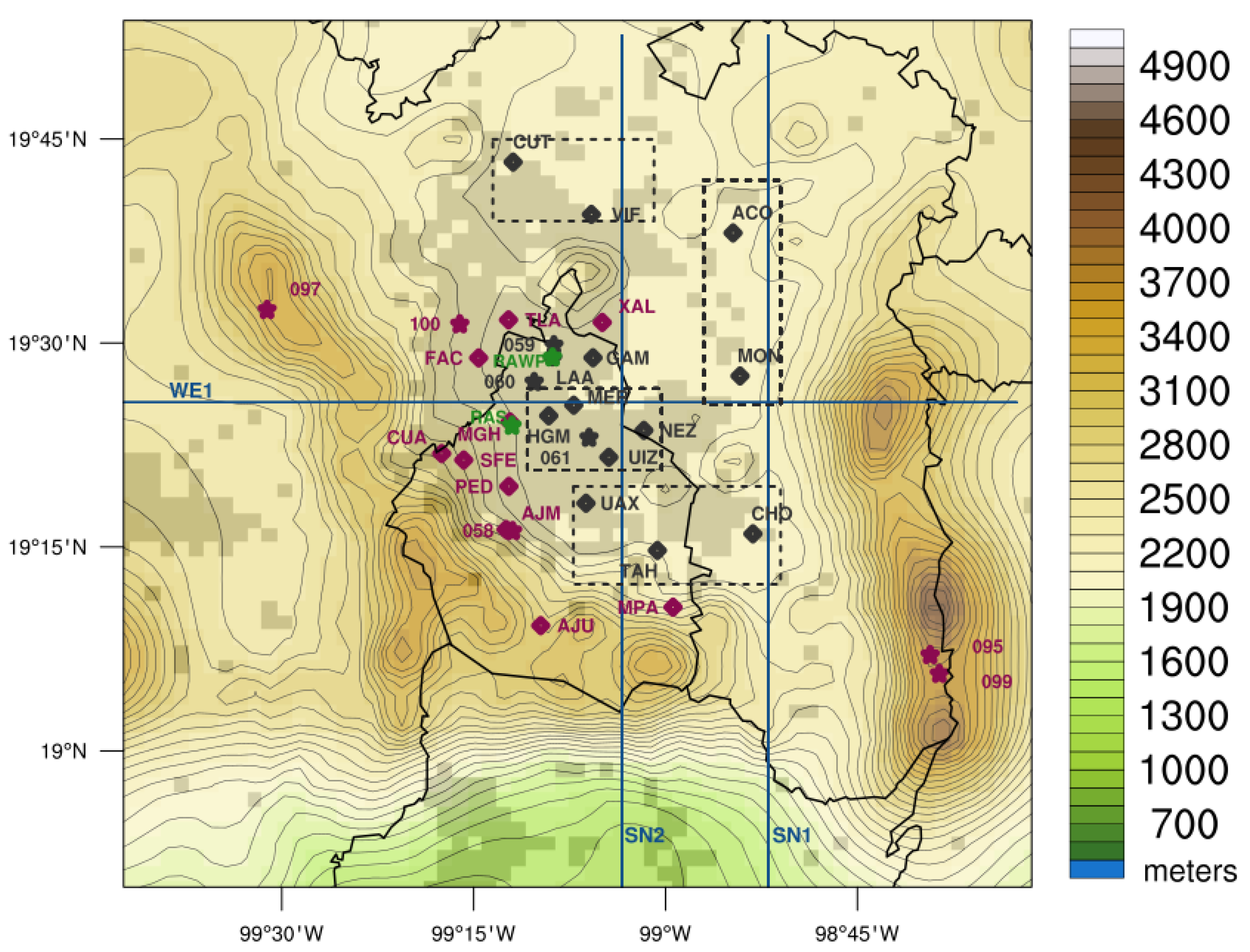
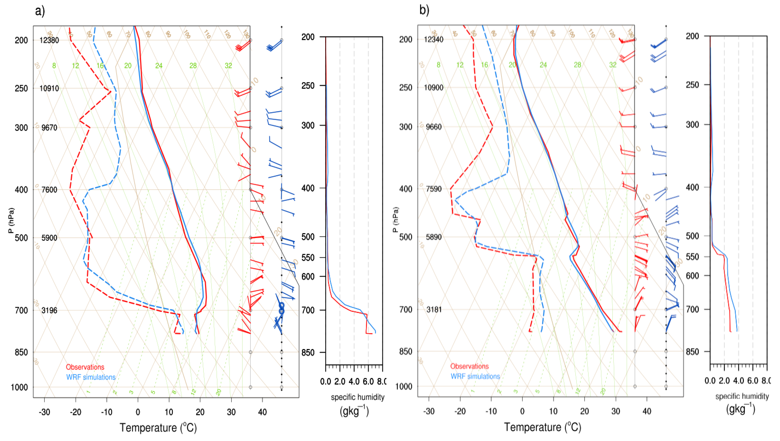
2.1. Terrain and Observational Data

The Mexico Basin’s important physiographic characteristics include its tropical location (20° N), high elevation (2250 m amsl), and the orographic confinement on its west and south sides by an almost continuous mountain chain with tops reaching about 3000 m agl. On its southeast corner, a mountain pass extends southward along the eastern mountains (Popocatépetl and Iztaccíhuatl) and connects it with a deep southern valley (Morelos Basin) 1000 m below (Figure 1). To the north, the Mexico Basin is open to the Sierra Madre Oriental and finally to the Gulf of Mexico, where it draws some of its moisture from the easterlies during the dry (winter) and wet (summer) seasons [20].
We use hourly surface meteorological variables from a network of 24 meteorological stations belonging to the Atmospheric Monitoring Agency of Mexico City (Secretaría del Medio Ambiente, SEDEMA). Additionally, 12 automatic meteorological stations maintained by the Mexican National Weather Service (Servicio Meteorológico Nacional, SMN) complete the observational surface network (Figure 1). Concerning upper levels, data is available from a 915 Mhz Doppler radar wind profiler (RAWP) (see Lau et al. [25] for technical details) maintained by SEDEMA. Note that the RAWP is located near the northern border of Mexico City limits (green dot in Figure 1) in a downward slope between two mountain ranges where a northwesterly gap wind usually develops. The RAWP outputs horizontal wind components as function of height above the basin floor and has an approximate vertical resolution of 60 m with a temporal resolution of 6 min and a range of about 3 km above ground level. Thus the RAWP can sample air well within the atmospheric boundary layer of the Mexico Basin. In addition, a radiosonde denoted here as RAS is available twice daily at 0600 and 1800 LST is launched from the headquarters of the SMN (lat: 19.4° long: 99.2° W elevation: 2313 m agl) in the northwest part of Mexico City (Figure 1). The surface database is subjected to a data quality control including time series homogeneization of temperature data. Table S1 (Supplementary Material) summarizes the surface station data. The air quality network from SEDEMA provides hourly ozone data. In addition to the above data, we use ECMWF ERA 5 reanalysis to analyze prevailing synoptic conditions and to obtain initial and boundary conditions for the regional atmospheric model as described below.

2.2. Case Study and Synoptic-Scale Conditions

The research focuses on the beginning of the warm period, which corresponds to February when the UHI intensity is higher in the Mexico Basin [16]. Due to availability of wind profiler data, the year 2017 is selected. To find days in February with weak synoptic conditions, we search days with the following restrictions: (1) ozone concentration values larger than 100 ppm (parts per million) as extracted from the SEDEMA air quality network, (2) zero precipitation from SMN rain gauge stations, (3) clear skies from solar radiation measurements at the SMN stations, and (4) adiabatic lapse rate with vertical gradients of potential temperature θ such that d θ / d Z > 9.8 K km 1 from the morning radiosonde at 0600 LST (see [20]). Vertical profiles of temperature, potential temperature, and adiabatic lapse rate for 9 February to 12 February are shown in Figure S1 of the Supplementary Material. All days show strong inversions at different levels in the vertical, but only 10 February stands out from the rest with the largest d θ / d Z = 10.2 K km 1 at about 690 m agl. On 10 February, average ozone concentrations show 125 ppm, and average direct solar radiation of 785 W m 2 for most SMN stations, which is near 90% of the theoretical average maximum value for the Mexico Basin on this date. Thus, 10 February meets all the above conditions best. Next, we analyze synoptic conditions for 10 February at 700 hPa and 500 hPa levels drawn from the ERA5 reanalysis data (see Figure S2 of Supplementary Material). At around 20° N, there is a well-defined ridge pattern precisely centered over the Mexico Basin at this time. This circulation pattern results from a mid-latitude Rossby wave train traveling westward with two deep troughs located in the Pacific and the Atlantic and a ridge in the middle over the central U.S. and Mexico. At 500 hPa, the geopotential height and wind patterns are very similar, with only minor changes in direction from its 700 hPa counterpart. While February climatology shows ridging over western North America and Mexico, the circulation pattern at hand, has its center shifted to the east relative to climatology (see https://psl.noaa.gov/cgi-bin/data/testdap/plot.comp.pl accessed on 22 May 2021) for an ERA5 rendering of geopotential height maps). One critical characteristic of this large-scale circulation pattern is the strong inversion over the Mexico Basin, which keeps air motions and humidity well confined within the atmospheric boundary layer.

2.3. WRF Modeling System

In this study, we use version 4.0 of the mesoscale atmospheric model system, Weather Research and Forecasting (WRF, [26]) to perform realistic and idealized simulations over the Mexico Basin. The one-way nested grid configuration consists of 3 domains (see Figure S3 of Supplementary Material) using a mesh spacing of 18 km in the external domain (D01), 6 km in the second domain (D02), and 2 km in the inner most domain (D03). The latter consists of 63 cells in the west-east direction and 60 cells in the north-south direction. This domain is designed to capture the orographically forced local phenomena and to avoid problems associated with the proximity to mountain ranges. All simulations use 76 sigma vertical levels, distributed as follows: 20 levels from the valley floor to 2250 m with about 50 m resolution for the first 5 levels, 30 levels between 2250 m and 6000 m, and the remaining 26 between 6000 m and 16,000 m. The choice of large vertical resolution is guided by the need to resolve within the atmospheric boundary layer the vertical structure of the wind system at the mountain slopes and the valley floor. The initial and lower boundary conditions of the numerical experiments are obtained from the ERA5 fifth generation of ECMWF atmospheric global reanalyses data which is available with a resolution of 0.25° × 0.25° starting from 1979, with a time resolution of every hour. The ERA5 is obtained from the Research Data Archive, which is maintained by the Computational and Information Systems Laboratory at the National Center for Atmospheric Research ([27]).

2.4. Model Configuration

The model is configured with the following physical parameterizations: The rapid radiative transfer model for global circulation models [28] is used to parameterize the longwave and shortwave radiation. The Kain-Fritsch scheme is selected for the representation of deep and shallow convection in the outer domain (the inner two domains have it turned off). The WSM6 scheme for cloud microphysics [29] is turned on in domain D03 only in order to account for possible orographic clouds. We use the Yonsei University (YSU) Planetary Boundary Layer (PBL) model ([30,31]), and the revised Noah land surface model LSM [32] coupled to a modified version of the Monin-Obukhov Similarity model for surface turbulent fluxes (see Section 2.6 for further discussion). The experiments start on 8 February at 0000 LST and end on 14 February at 2300 LST, with model output every 10 min. The first 24 h are not considered in the analysis since they are part of the required model spin-up. The WRF model provides two LULC alternative databases: the U.S. Geological Survey (USGS), LULC database, generated in 1993, and the Moderate Resolution Imaging Spectroradiometer (MODIS) database, generated in 2001. Both datasets are not updated and are not accurate for all regions and some land cover types, such as urban areas ([33,34,35,36]). In atmospheric modeling, an accurate representation of LULC is key because such information impacts the correct estimate of water and energy fluxes, the atmospheric circulation, and consequently, the quality of regional climate and weather simulations. The National Institute of Statistic and Geography (Instituto Nacional de Estadística y Geografía, INEGI) is the federal agency that gathers and distributes Mexico’s LULC information which can be downloaded from its web page (https://www.inegi.org.mx/temas/usosuelo accessed on 27 January 2021). Serie-VI represents the latest LULC maps produced for Mexico with a far more reliable LULC description than those currently available for the WRF model. To obtain a proper LULC for WRF, we reclassify the Serie-VI LULC into the 24 USGS defined categories while including the particular phenological and geographical characteristics of the INEGI vegetation types. Lastly, we match Serie-VI´s coordinate system and spatial resolution to the original USGS’s LULC (see [37] for technical details).

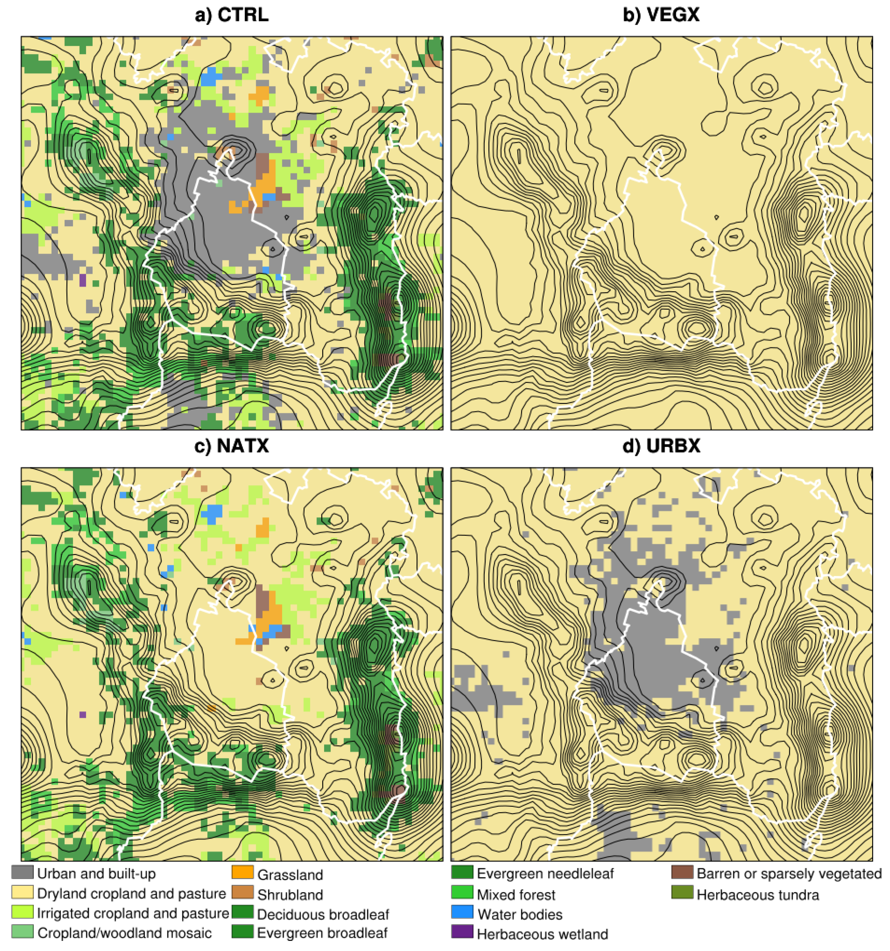
2.5. Control and Hypothesis Testing Experiments

Figure 2a shows domain D03 (see Figure 1) with the new LULC data from INEGI for the control (CTRL) experiment. Three LULC categories (Figure 2b–d) stand out, as far as area cover: the urban and built-up category with 16%, the dryland cropland, and pasture (denoted DCP, hereafter) with 51%, and evergreen needleleaf forest with 12.6%. Table 1 shows all the LULC categories and their percent area cover.
To explore the urban effect (UE) on local circulation and UHI development, we propose three hypothesis testing experiments in the D03 domain with modified LULC from the CTRL experiment: (1) VEGX experiment, where the LULC from the CTRL is replaced completely by the DCP LULC category (2) URBX experiment, same as VEGX except that the CTRL’s urban and built-up category is superposed onto the VEGX’s DCP category, and (3) NATX experiment, same as CTRL but with its urban and built-up LULC category replaced by the dominant DCP category. For comparison, Figure 2 shows, the geographical distribution of LULC in the hypothesis testing experiments described above, including the CTRL. The CTRL and the three hypothesis testing help define two meaningful UE: the difference (CTRL-NATX) is the UE keeping the LULC heterogenous, and the difference (URBX-VEGX) is the UE keeping the LULC homogeneous (since the DCP category is in both URBX and VEGX). The hypothesis behind these two UEs is that the difference (CTRL-NATX) is more complex than its counterpart (URBX-VEGX) since inhomogeneous LULC surface conditions can generate mesoscale eddies within the PBL that can impact the local circulation effectively. To further investigate the UE on the three dimensional local circulation patterns in the Mexico Basin we use moist static energy ( M S E ) defined as: M S E = C p T + g z + L v q , where L v is the latent heat of vaporization (2.5 × 10 6 J kg 1 ), q the specific humidity, and C p T is enthalpy (J kg 1 ) and g z is potential energy per unit mass. M S E is conserved following non-condensing adiabatic motion of the parcels [38]. Synoptic and local circulations for this case study restrict the conversion of water vapor into condensed water(except possibly during ascend of moist air up the mountain slopes), and the only significant sources or sinks of water vapor q and M S E lie at the lower boundary and the lateral walls of the computational volume domain of the model.

2.6. Model Parameterization Tests

In order to obtain the best configuration of physical parameterizations available from WRF we use the following statistical measures of distance between simulations and observed fields: (i) the root mean square error (RMSE), (ii) the correlation coefficient (R) and (iii) the bias (B) ([39,40] for details). The results of the comparisons between the different parameterizations are shown using Taylor diagrams which facilitate the interpretation of statistical metrics in a compact form, with the added advantage of analyzing several variables in a single diagram. The statistical metrics for simulated and observed quantities in the Taylor diagram are:
R M S E = i = 1 N ( M V i O V i ) 2 N ,
R = 1 N 1 i = 1 N M V i μ M σ M O V i μ O σ O ,
B = 1 N i = 1 N M V i O V i ,
where R M S E is root mean square error, R is the Pearson pattern correlation, B is the bias, M V i and O V i are the modeling and observation variables respectively closest to the i t h observational site and N is the total number of observational sites considered. The μ and σ are the mean and standard deviations of the corresponding model and observed variable, respectively.
Several PBL turbulence schemes are tested in WRF to estimate the above statistical measures (not shown). Simulations with WRF underestimate wind magnitude in the Mexico Basin and it remains a challenge and an open question that is being pursued at the moment. For this reason, the choice is to minimize the error in wind direction rather than its magnitude. Table S3 in Supplementary Material shows the Taylor metric for temperature and the horizontal wind components. The revised YSU PBL model produces, on average, a Pearson correlation of about 0.5 in wind direction for the diurnal cycle. Other choices for PBL such as Mellor-Yamada 8 [41,42]), Mellor-Yamada-Niino ([43,44]) and Total Energy-Mass Flux [45] show lower Pearson correlation values (not shown).

3. Results and Discussion

3.1. CTRL Simulation

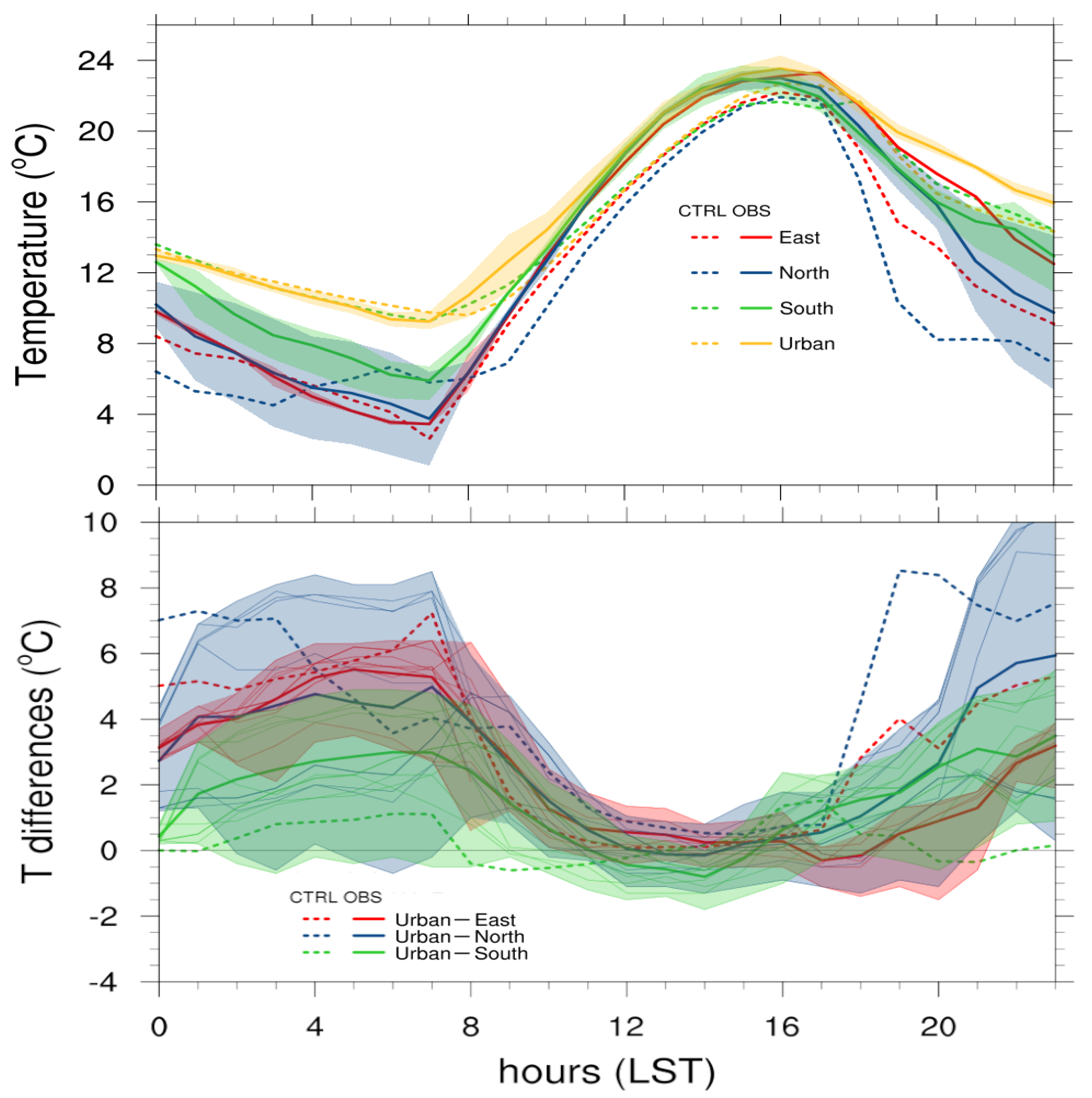
3.1.1. UHI Intensity, and Humidity

Figure 3 upper panel shows the hourly comparison between the observed and the simulated diurnal cycle of temperature from four selected areas within the Mexico Basin: East, North, South, and Urban (see dotted rectangles in Figure 1). Each area temperature is the average temperature from several SMN weather stations within each area according to elevation while model data corresponds to the closest grid-point to the station location. Stations below 2300 m amsl correspond only to the Urban area. The model captures the temperature evolution of the Urban area for the most part of the day except for the late evening hours (1900 to 2300 LST) when a cold bias of about 3 °C develops. Over the East and North areas the model temperature falls well within the spatial variability early in the morning, and shows a persistent cold bias of about 2 °C, starting at 0700 LST which grows to 5 °C, in the late evening hours. A warm bias of about 4 °C for the South area is present in the early morning hours that tends to diminish later in the afternoon. Despite the fact that SMN stations have very similar elevations for each area, it is interesting to note that there are temperature deviations among them early in the morning and late at night. This behavior is particular to the South, North and East areas and not so much for the Urban area. Figure 3 lower panel shows the UHI intensity as the temperature difference between the Urban area with the East, West, and South areas. In general, the model UHI intensity falls within the spatial variability bands of the observed data with the exception of the North area which has a much stronger positive UHI than observed in the evening hours. This result is consistent with the rather strong cold bias of the North area compared to the Urban area, as shown in Figure 3 upper panel. One possible explanation for the model excessive intensification of the positive UHI between the Urban and North areas is attributed to the orographic blocking of cold low-level northerly wind by a mountain chain in the middle of the Mexico Basin (Sierra Guadalupe, see Figure 1). Another important feature to notice of the UHI is the onset and end of cold pools between the Urban area, and the South and East areas. The cold pool between Urban and South starts at 1100 LST and further along, north of the Chalco pass, the cold pool between Urban and East starts at about 1600 LST. In the late afternoon, after 1800 LST the UHI between Urban and East areas increases signaling the arrival of cold air from the south at the South area near the Chalco pass. This phenomenon has been linked in the past to the advection of cold air by low-level south-westerly jet from the surrounding basins towards the warm Mexico Basin as discussed at some length by previous authors ([18,20,23]), and will be further discussed in the context of the Mexico Basin wind system. Figure 3 lower panel also shows the distinct positive UHI to occur from about 1800 LST of the previous day until around noon for all areas.
Figure 4 shows the radiosoundings for 0600 LST and 1800 LST and the corresponding sounding from the CTRL experiment. As expected, the ridging over the Mexico Basin is evident in both the SMN and the model simulation. At 0600 LST, the SMN sounding shows a temperature inversion located at about 700 hPa (880 m agl). At 1800 LST, the inversion height is at about 547 hPa (2871 m agl). The model captures the amplitude and height of the inversion quite well in the PBL. Figure 4 also shows the vertical profile for the observed and model specific humidity. At 0600 LST, both, SMN and model, show a shallow humid (relative to values above 2871 m agl) and cold layer of about 6 g kg 1 and 7 °C on average. At this hour, the model and the SMN specific humidity values are very close to each other near the surface, but the model shows a more gradual drop in specific humidity compared to the SMN sounding. At 1800 LST, SMN specific humidity values range from about 3.7 g kg 1 near the surface, to 2.1 g kg 1 below and near an inversion level height of about 2870 m agl. Figure 4 also shows the model to be somewhat more humid than observed by about 1.0 g kg 1 . The simulation of the horizontal wind components is well captured in amplitude and pattern by the model, with westerlies above the 400 hPa level and easterlies below that level at 0600 and 1800 LST. Notably, at 0600 LST, below the 700 hPa level, in both model and observations a northwesterly wind flows down the slope towards the city center. Neighboring surface SMN stations agree in general with this early morning low-level wind field and report a shift to northeasterlies between midday and later in the evening (not shown).

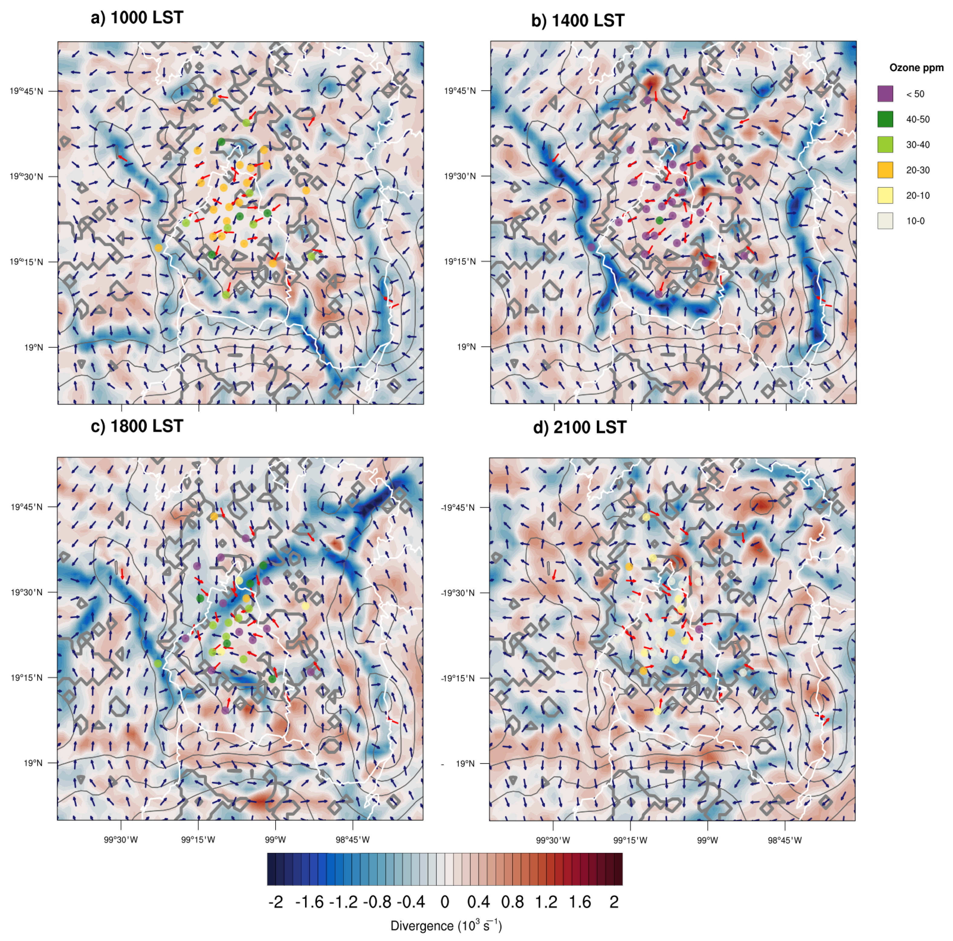
3.1.2. Near-Surface Wind Field, Wind Convergence Lines, and Ozone Measurements

Figure 5 shows selected times (1000, 1400, 1900 and 2100, LST) on 10 February 2017, for the CTRL simulation wind field at 10 m agl (black vectors) and the corresponding observed wind field at 10 m agl from 28 available weather stations (red vectors) over the Mexico Basin. Figure 6 also shows narrow bands (or lines) of surface wind convergence from model data. At 1000 LST, Figure 5a shows a low-level northerly Chalco jet in the southeastern corner of the Mexico Basin, flowing towards the Morelos Basin in its southern border. North of the basin, there are northeasterly winds towards the southern mountain chain in the model, and in the observations as well. In addition, the model shows distinct upslope winds at both flanks of the mountain chains forming convergence lines over the mountain crests. At 1400 LST the Chalco jet changes to northerly direction in the model (Figure 5b), and although there is no observational site to confirm this event directly, the reversed direction is consistent with the observed increment in the UHI intensity after 1400 LST for the East area, as discussed earlier in the previous section. The model and observed wind vector data agree in direction quite well at this time, although the model at times underestimates quite significantly the magnitude of the wind (see Taylor diagram Figure S4 in Supplementary Material). In order to emphasize wind direction over wind magnitude in the horizontal maps, the norm of all vectors (observed and modeled) is set to one unitless magnitude. The wind system shows a dominant northerly wind component and upslope winds in all mountain chains surrounding the basin at this time as well. At 1900 and 2100 LST a thermally induced pressure gradient (from a warmer elevated basin and colder surroundings) generates northeasterly winds north of the basin (Figure 5c,d). At these times, radiational cooling from the southern mountain slopes induces downslope winds which join the southerly wind from Chalco and push through the entire basin creating strong south-west, north-east oriented convergence lines in the middle of the basin at the northern city limits. Note that, previous to the arrival of convergence lines in the middle of the basin (Figure 5b), ozone level concentrations are larger than 50 ppm, with some stations reporting values of about 100 ppm (not shown), and only start to decline to 40 and 30 ppm at around 1800 LST when convergence lines finally arrive there. The observed dilution of ozone concentrations is associated not only to turbulent mixing but also to vertical transport induced by horizontal convergence, as will be discussed in the next section.
Figure 6 shows the hourly horizontal wind components as a function of height for the February 10 case study by the RAWP in the north east of the basin (See Figure 1). Figure 6 also shows the CTRL simulation for the nearest grid point to the RAWP location. Note that the RAWP reports wind field data up to different height levels during the sampling period. The CTRL simulation at the RAWP site shows a well defined transition line characterized by a sharp veering from westerlies to easterlies whose height reaches a maximum of 2200 m agl at 1700 LST. At low levels, in the early morning hours, low-level northwesterly and westerly winds are present on both, the RAWP and the CTRL simulation, however the RAWP shows a more sustained westerly wind for almost the whole sampling period. Two near weather stations (LAA and 059, see Figure 1) report wind directions which agree more with the CTRL simulation. At upper levels, both the CTRL simulations and the RAWP agree on the easterly wind direction up until midday. After 1200 LST the CTRL and RAWP differ on the wind direction, which is interesting since the SMN radiosounding does not agree with the RAWP, as well. The reason for these discrepancies in wind direction is not clearly known, at this stage of the investigation. In general, however, we deem acceptable the performance of the model CTRL simulation when compared to available observations for this case study.

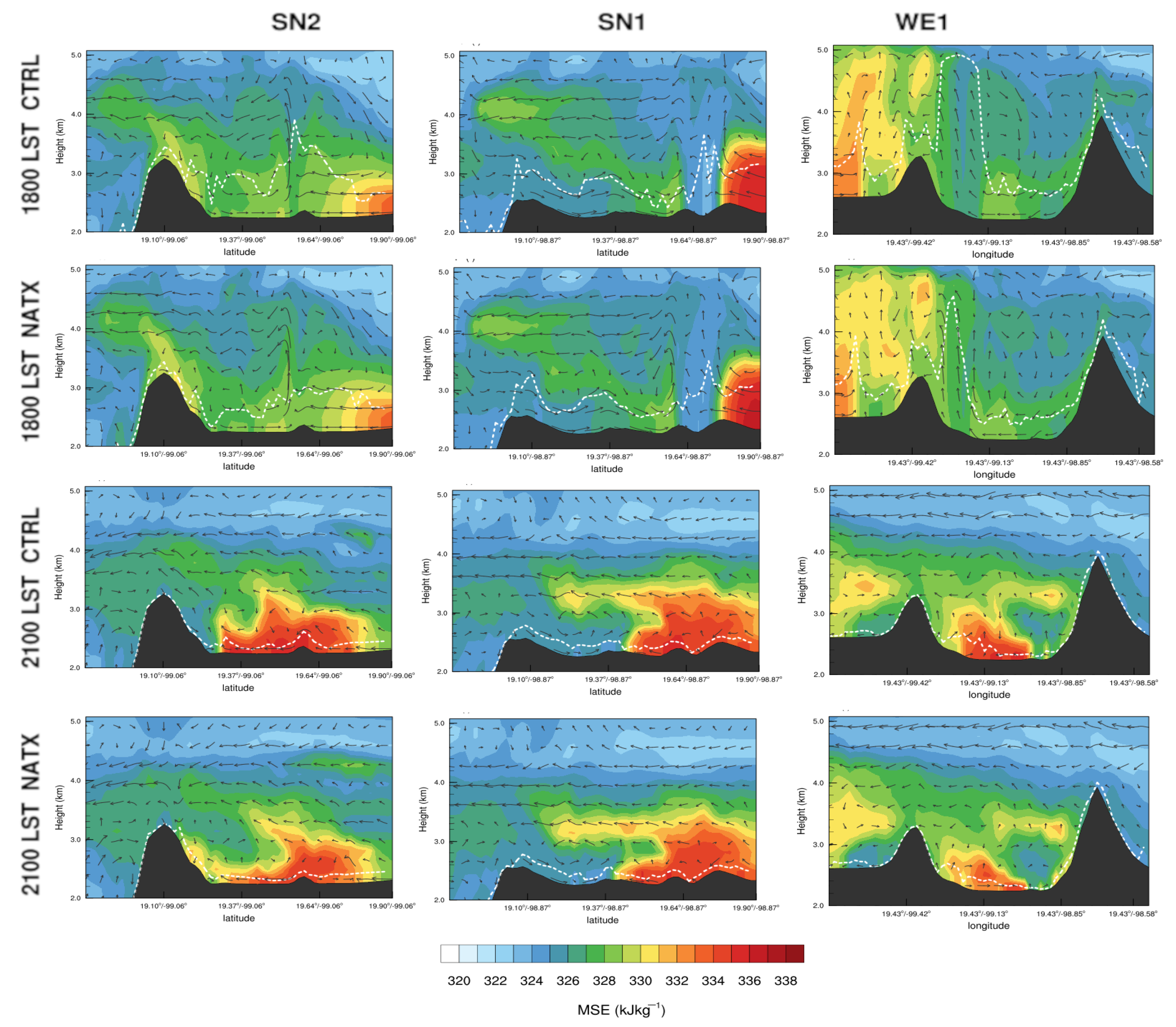
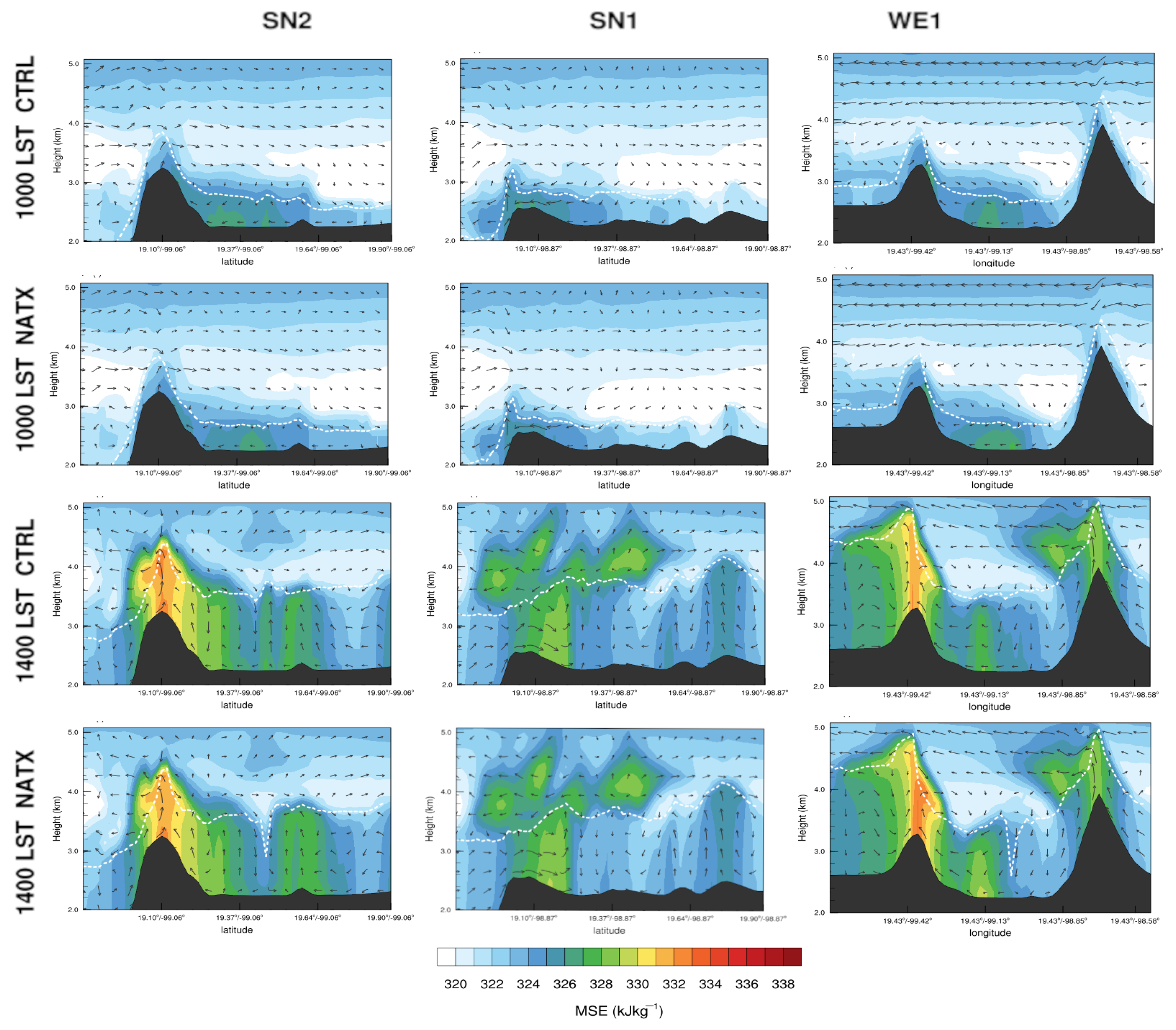
4. Urban Effects on Circulation and MSE

Figure 1 shows three transects, two in the south-north direction: SN1 (lon: 98.87° W), and SN2 (lon: 99.06° W) in the east and center of the Mexico Basin, respectively. Finally, we add a third west-east transect WE1 (lat: 19.43° N) in the middle of the basin. Based on these three transects, Figure 7 shows M S E and wind field as a function of height and latitude for the CTRL simulation and the NATX experiment at 1000, and 1400 LST. At 1000 LST both, CTRL and NATX, display a similar behavior in wind and M S E fields. In all transects, there is air subsidence that keeps relative larger values (with respect to background) of M S E below 600 m agl. Upslope winds develop in all transects except in SN1 which shows a southerly low-level jet (the Chalco jet) advecting high values (relative to background) of M S E air into the Morelos Basin, south of the Mexico Basin. At the same time, however, there is an upslope wind from the Morelos Basin underneath converging with drainage flow at the crest of the Chalco pass. At 1400 LST the PBL reaches heights of about 1100 m over the floor’s basin. Upslope winds continue in all transects except on SN1 where now the Chalco jet veers to southerly wind, and changes in M S E become more discernible between the CTRL and NATX. SN1, and SN2 show, on average, air parcels with low M S E below the PBL in the NATX experiment compared to CTRL due to more intense subsidence of low M S E parcels in the NATX experiment, particularly over the Chalco pass. At this time, the WE1 transect shows a circulation pattern that reminds of idealized two-dimensional simulations [46] with sinking motions in the middle of the basin and upslope wind at the mountain chains facing the basin. The CTRL experiment shows a larger PBL height compared to NATX and less intense subsidence of parcels with low M S E values on the eastern flank. Nevertheless, there is a remarkable asymmetry in the circulation that results from larger heating on the western mountain chain compared to that in the east [4]. Furthermore, at WE1, values of M S E for the CTRL are smaller than those of NATX, particularly near the surface. This decrease in M S E is related to larger latent heat fluxes in the NATX experiment as is discussed further below.
Figure 8 shows M S E and wind fields at 1800, and 2100 LST, when the UHI becomes fully developed in the CTRL simulation as discussed previously in Section 3.1.1. At 1800 LST, near-surface convergence lines develop in the middle of the basin with a southeast-northwest slant due to air masses converging from the north and the south. Transect SN2, shows a convergence line at about 19.55° N while SN1 shows two convergence lines separated by a region of low values of M S E air at about 19.70° N (see also Figure 5). SN1 shows the Chalco jet carrying air with low values of M S E (325 kJ kg 1 ) which lowers the PBL height to the north. From the north, air masses with higher values of M S E (335 kJ kg 1 ) have higher humidity content than the southern air masses (not shown). At this time, the WE1 transect shows a zonal circulation that has evolved from earlier hours into a full convection cell transporting air parcels downward with lower values of M S E from aloft, on the eastern side of the basin, and upslope winds on its western side. The CTRL simulation is characterized by a stronger zonal circulation with larger PBL heights than the NATX experiment. At 2100 LST, transects SN1, and SN2 show the northern air mass reaching the southern basin carrying high values of M S E particularly below the PBL which is quite shallow with PBL heights of about 200 m agl for the CTRL and about 100 m agl for NATX. Of note is the more confined nature of air parcels within the basin in the CTRL simulation compared to those in the NATX experiment. This is associated to a stronger downslope wind carrying down air parcels with low M S E values until converging at the piedmont with higher M S E air impeding further advance towards the south. On the other hand, NATX shows air parcels upslope. At this time, the WE1 transect for the CTRL simulation shows convergence in the middle of the basin over the urban built-up area with ascending motion, as is clear from the M S E and wind fields. The WE1 transect for NATX fails to develop a similar wind and M S E patterns since, in this case, air parcels are more vertically confined. At this point in time (in contrast to 1400 LST, see Figure 7), M S E values are lower in the WE1 transect for the NATX experiment compared to the CTRL simulation with larger differences closer to the surface. This change in MSE is mostly related to higher MSE values from larger enthalpy near the ground in the CTRL compared to NATX. Figures S5 and S6 in Supplementary Material shows the corresponding transects for the URBX and VEGX experiments. These are all quite similar in pattern to their CTRL, and NATX counterpars. In magnitude, however, differences in M S E between the URBX and VEGX are more discernible and less noisy, and not so much, as far as wind field is concerned.
Figure 9 shows, the UE as differences between the CTRL and NATX experiments in latent heat flux (LHF), sensible heat flux (SHF), ground flux (GRF), and net radiation at the surface (RNET). We interpret (following [47] p. 251) positive fluxes as going into the atmosphere and negative otherwise. In the morning-afternoon (1000, and 1400 LST) the RNET difference is negative implying, that RNET for NATX is larger (i.e., less negative) than RNET for the CTRL. At this time, SHF is positive for both CTRL and NATX, and very close to each other in magnitude at 1000 LST. However, at 1400 LST, the SHF of CTRL surpasses that of NATX by about 40 W m 2 as Figure 9 shows in the SHF panels. At this time, the LHF in the CTRL simulation is very small in absolute value while that of the NATX experiment is positive (not shown) leading to negative differences in LHF between the CTRL and NATX simulations. At 1400 LST this negative difference in LHF increases. This increase in LHF is in agreement with larger values of M S E near the surface as Figure 7 shows for NATX at 1400 LST. Next, we examine the night period (1800, and 2100 LST). The positive difference in SHF implies the CTRL has a larger SHF than NATX, as expected, during this part of the diurnal cycle with values larger than 45 W m 2 with maxima at 1800 LST as Figure 9 shows in the SHF column. The response in M S E can be seen in all transects at 2100 LST with larger values of M S E for the CTRL near the surface compared to NATX (see Figure 7). Finally, the UE in this very simple model of urban area is interpreted as the difference in energy storage by the urban and built-up category in the CTRL and the NATX experiment. In the morning-afternoon period, the GRF is negative, and Figure 9 shows the CTRL to be more negative than NATX as expected since the urban and built-up area is expected to store more energy than the DCP category during the day. At night, the GRF becomes positive for both CTRL and NATX experiment but this time, the difference in GRF is positive meaning that the urban and built-up area is giving off energy to the atmosphere at a greater rate than the DCP category. Figure S7 in Supplementary Material shows the homogeneous UE for the URBX and VEGX experiments.

5. Summary and Conclusions

The present work tests the hypothesis that changes in LULC significantly impact local circulation in the Mexico Basin, particularly near-surface wind field circulations such as gap winds, convergence lines, and thermally induced upslope/downslope wind at the foot of mountain chains. Many past modeling studies on urban heat islands support this hypothesis (e.g., [2,46]). Our results confirm this, albeit with some caveats due to the complex topography and synoptic forcing that characterizes the Mexico Basin. In order to isolate the influence of large-scale synoptic forcing, we select 10 February 2017, as a special case study with a very well-defined high-pressure system over the Mexico Basin at the center of the country. This case study selection permits a convincing simulation of the main physical processes at work. It isolates the influence that LULC has on the wind system and the thermodynamics based on hypothesis testing experiments where LULC changes from the control simulation. Thus, we interpret the urban effect regarding the differences between the control and the hypothesis testing experiments. The control simulation reveals a three dimensional wind pattern composed of: (i) meridional (south-north) circulations driven by the thermal pressure gradients between the high plateau of the Mexico Basin and surrounding coastal areas (see Figure S5 in Supplementary Material), and (ii) a zonal (west-east) upslope/downslope circulation driven by the thermal interaction with the urban and built-up area and the heating/cooling of the mountain slopes facing the basin. The sense of the meridional circulation depends on the change of pressure gradients between the Mexico Basin and its surroundings as the basin warms and cools faster than its surroundings. The replacement of the natural and cultivated land by urban and built-up areas leads to more organized meridional and zonal circulations inside the basin, particularly in the afternoon and night times when the UHI intensity is largest. Near-surface wind convergence lines in the afternoon connect with the upper air circulation and not only help close the meridional circulation but mark the border between two distinct air masses: one with low M S E advected from the south and another with high M S E advected from the north. At this time, downslope wind from the southern mountains and Chalco jet complete the low-level wind meridional circulation branch. This type of circulation helps redistribute the M S E or passive tracers originating at the basin floor vertically and export them to the southern basin (Morelos Basin) or returning them to the basin. Results from hypothesis testing experiments with natural and cultivated areas indicate a similar meridional circulation albeit less organized and with lower PBL heights. In the afternoon, the zonal circulation exhibits a typical circulation pattern with upslope flow on both of the flanking mountains, and descending motion over the Chalco pass. Also there is a zonal asymmetry with lower M S E over the Chalco pass and larger M S E on the western side of the basin. The experiment with natural cover only, shows a more accentuated asymmetry than the control. The controls that the land use land cover exert upon the circulation result in larger values of M S E near the surface where air parcels pick up energy from the surface either in the form of fluxes of enthalpy or latent heat. Surface heat fluxes and stored energy in the ground are drivers of local circulation which is more evident in zonal circulation patterns. One surprising result from this work is the generation of convection cells at the basin scale in the afternoon. One would expect that given the low ratio of mountain height to basin horizontal length (0.03 on average), the UHI circulations would be disconnected from the upslope and downslope winds. Rendón et al. [48] in an idealized two-dimensional experiment with a 0.06 ratio find that the UHI circulations are closely linked to the upslope/downslope wind system. It would be interesting to explore in, the more complex topography context of the Mexico Basin, if there is a lower limit to this ratio where UHI circulations and upslope/downslope winds are decoupled from each other. Finally, this work opens up another important avenue of research in regards to the thermal pressure gradients as the main driver of near-surface wind divergence/convergence, and circulation within the Mexico Basin. This dynamical ingredient is required if we are to understand how large-scale variability during the dry season affects the mesoescale circulations within the basin. These type of research is of high relevance to air quality studies for the basin. The present work is a first in a series of research works dedicated to understand in detail the interactions of the Mexico Basin circulation patterns and its urban landscape.

Supplementary Materials

The following are available online at https://www.mdpi.com/article/10.3390/atmos12070904/s1, Figure S1: Vertical profiles, Figure S2: Synoptic charts, Figure S3: Computational domains, Figure S4: Day-time MSE vertical cross-sections for URBX and VEGX, Figure S5: Night-time MSE vertical cross-sections for URBX and VEGX. Figure S6: Same as Figure S5, except for 1800 and 2100 LST, Figure S7: Urban effect as the difference in energy fluxes W m 2 at the surface between the URBX simulation and the VEGX experiment for February 10 at 1000, 1400, 1800, and 2100 LST. Columns 1, 2, 3 and 4 are for latent heat fluxes (LHF), sensible heat fluxes (SHF), ground flux (GRF), and net radiation, respectively. Positive direction for fluxes implies atmosphere receives energy from the surface below. Table S1: Stations locations, Table S2: Station Taylor metrics, Table S3: Hourly Taylor metrics.

Author Contributions

A.I.Q. and L.P.A.-M. conceptualized the idea and wrote the first draft of the paper. L.P.A.-M. worked in code development. All authors contributed to the interpretation of the results and to the writing of the paper. All authors have read and agreed to the published version of the manuscript.

Funding

Aquino-Martínez was funded with scholarships from Mexican National Council for Science and Technology (CONACyT) number 331962.

Data Availability Statement

Model simulation output data are available on request from L.P.A.-M. ([email protected]).

Acknowledgments

We thank two anonymous reviewers, for valuable comments that significantly improved the manuscript. We thank the SEDEMA and SMN for providing the data. All figures were generated with The NCAR Command Language (Version 6.6.2) [Software]. (2019). Boulder, CO, USA: UCAR/NCAR/CISL/TDD, doi:10.5065/D6WD3XH5.

Conflicts of Interest

The authors declare no conflict of interest.

Abbreviations

The following abbreviations are used in this manuscript:
aglabove ground level
amslabove mean sea level
BBias
CONACyTMexican National Council for Science and Technology
CTRLControl experiment
DCPDryland cropland and pasture
ECMWFEuropean Centre for Medium-Range Weather Forecasts
ERA 5ECMWF Reanalysis v5
GRFGround Flux
INEGINational Institute of Statistics and Geography
LHFLatent Heat Flux
LSTLocal standard time
LULCLand Use Land Cover
MODISResolution Imaging Spectroradiometer
MSEMoist Static Energy
NATXNatural vegetation experiment
SN1south-north transect at 98.87° W
SN2south-north transect at 99.06° W
PBLPlanetary Boundary Layer
ppmparts per million
RCorrelation Coefficient
RASRadiosonde
RAWPRadar Wind profiler
RMSERoot Mean Square Error
RNETNet Radiation
SEDEMAAtmospheric Monitoring Agency of Mexico City
SHFSensible Heat Fluxes
SMNServicio Meteorológico Nacional
UEUrban Effect
UHIUrban Heat Island
UNAMUniversidad Nacional Autónoma de México
URBXUrban experiment
USGSU.S. Geological Survey
VEGXVegetated experiment
WE1West-East transect at 19.43°N
WRFWeather Research and Forecasting

References

  1. Miao, S.; Chen, F.; LeMone, M.A.; Tewari, M.; Li, Q.; Wang, Y. An observational and modeling study of characteristics of urban heat island and boundary layer structures in Beijing. J. Appl. Meteorol. Climatol. 2009, 48, 484–501. [Google Scholar] [CrossRef]
  2. Ganbat, G.; Baik, J.J.; Ryu, Y.H. A numerical study of the interactions of urban breeze circulation with mountain slope winds. Theor. Appl. Climatol. 2015, 120, 123–135. [Google Scholar] [CrossRef]
  3. Wang, D.; Miao, J.; Zhang, D.L. Numerical simulations of local circulation and its response to land cover changes over the Yellow Mountains of China. J. Meteorol. Res. 2015, 29, 667–681. [Google Scholar] [CrossRef]
  4. Rendón, A.M.; Salazar, J.F.; Palacio, C.A.; Wirth, V. Temperature inversion breakup with impacts on air quality in urban valleys influenced by topographic shading. J. Appl. Meteorol. Climatol. 2015, 54, 302–321. [Google Scholar] [CrossRef]
  5. Ding, Y.; Peng, J. Impacts of urbanization of mountainous areas on resources and environment: Based on ecological footprint model. Sustainability 2018, 10, 765. [Google Scholar] [CrossRef] [Green Version]
  6. Edgerton, S.A.; Bian, X.; Doran, J.; Fast, J.D.; Hubbe, J.M.; Malone, E.L.; Shaw, W.J.; Whiteman, C.D.; Zhong, S.; Arriaga, J.; et al. Particulate air pollution in Mexico City: A collaborative research project. J. Air Waste Manag. Assoc. 1999, 49, 1221–1229. [Google Scholar] [CrossRef] [PubMed] [Green Version]
  7. Pielke, R.A. Land use and climate change. Science 2005, 310, 1625–1626. [Google Scholar] [CrossRef] [Green Version]
  8. Bornstein, R.D. Observations of the urban heat island effect in New York City. J. Appl. Meteorol. Climatol. 1968, 7, 575–582. [Google Scholar] [CrossRef]
  9. Bornstein, R. Mean diurnal circulation and thermodynamic evolution of urban boundary layers. Model. Urban Bound. Layer 1987, 53–93. [Google Scholar]
  10. Oke, T. The heat island of the urban boundary layer: Characteristics, causes and effects. In Wind Climate in Cities; Springer: Dordrecht, The Netherlands, 1995; pp. 81–107. [Google Scholar]
  11. Zak, M.; Nita, I.A.; Dumitrescu, A.; Cheval, S. Influence of synoptic scale atmospheric circulation on the development of urban heat island in Prague and Bucharest. Urban Clim. 2020, 34, 100681. [Google Scholar] [CrossRef]
  12. Beck, C.; Straub, A.; Breitner, S.; Cyrys, J.; Philipp, A.; Rathmann, J.; Schneider, A.; Wolf, K.; Jacobeit, J. Air temperature characteristics of local climate zones in the Augsburg urban area (Bavaria, southern Germany) under varying synoptic conditions. Urban Clim. 2018, 25, 152–166. [Google Scholar] [CrossRef]
  13. Półrolniczak, M.; Kolendowicz, L.; Majkowska, A.; Czernecki, B. The influence of atmospheric circulation on the intensity of urban heat island and urban cold island in Poznań, Poland. Theor. Appl. Climatol. 2017, 127, 611–625. [Google Scholar] [CrossRef] [Green Version]
  14. Jauregui, E. Mexico City’s urban Heat Island revisited (die Wärmeinsel von Mexico City—Ein Rückblick). Erdkunde 1993, 47, 185–195. [Google Scholar] [CrossRef]
  15. Jauregui, E. Heat island development in Mexico City. Atmos. Environ. 1997, 31, 3821–3831. [Google Scholar] [CrossRef]
  16. Cui, Y.Y.; De Foy, B. Seasonal variations of the urban heat island at the surface and the near-surface and reductions due to urban vegetation in Mexico City. J. Appl. Meteorol. Climatol. 2012, 51, 855–868. [Google Scholar] [CrossRef]
  17. Klaus, D.; Jauregui, E.; Poth, A.; Stein, G.; Voss, M. Regular Circulation Structures in the Tropical Basin of Mexico City as a Consequence of the Urban Heat Island Effect (Regelhafte Zirkulationsstrukturen im tropischen Hochbecken von Mexiko Stadt als Folge des Wärmeinseleffektes). Erdkunde 1999, 231–243. [Google Scholar] [CrossRef]
  18. Jazcilevich, A.D.; García, A.R.; Ruíz-Suárez, L.G. A study of air flow patterns affecting pollutant concentrations in the Central Region of Mexico. Atmos. Environ. 2003, 37, 183–193. [Google Scholar] [CrossRef]
  19. Jazcilevich, A.D.; García, A.R.; Caetano, E. Locally induced surface air confluence by complex terrain and its effects on air pollution in the valley of Mexico. Atmos. Environ. 2005, 39, 5481–5489. [Google Scholar] [CrossRef]
  20. Whiteman, C.; Zhong, S.; Bian, X.; Fast, J.; Doran, J. Boundary layer evolution and regional-scale diurnal circulations over the and Mexican plateau. J. Geophys. Res. Atmos. 2000, 105, 10081–10102. [Google Scholar] [CrossRef]
  21. de Foy, B.; Caetano, E.; Magana, V.; Zitácuaro, A.; Cárdenas, B.; Retama, A.; Ramos, R.; Molina, L.; Molina, M. Mexico City basin wind circulation during the MCMA-2003 field campaign. Atmos. Chem. Phys. 2005, 5, 2267–2288. [Google Scholar] [CrossRef] [Green Version]
  22. de Foy, B.; Clappier, A.; Molina, L.; Molina, M. Distinct wind convergence patterns in the Mexico City basin due to the interaction of the gap winds with the synoptic flow. Atmos. Chem. Phys. 2006, 6, 1249–1265. [Google Scholar] [CrossRef] [Green Version]
  23. Doran, J.; Zhong, S. Thermally driven gap winds into the Mexico City basin. J. Appl. Meteorol. 2000, 39, 1330–1340. [Google Scholar] [CrossRef]
  24. Kimura, F.; Kuwagata, T. Thermally induced wind passing from plain to basin over a mountain range. J. Appl. Meteorol. Climatol. 1993, 32, 1538–1547. [Google Scholar] [CrossRef]
  25. Lau, E.; McLaughlin, S.; Pratte, F.; Weber, B.; Merritt, D.; Wise, M.; Zimmerman, G.; James, M.; Sloan, M. The DeTect Inc. RAPTOR VAD-BL radar wind profiler. J. Atmos. Ocean. Technol. 2013, 30, 1978–1984. [Google Scholar] [CrossRef]
  26. Skamarock, W.C.; Klemp, J.B.; Dudhia, J.; Gill, D.O.; Liu, Z.; Berner, J.; Wang, W.; Powers, J.G.; Duda, M.G.; Barker, D.M.; et al. A Description of the Advanced Research WRF Model Version 4; National Center for Atmospheric Research: Boulder, CO, USA, 2019; p. 145. [Google Scholar]
  27. Hersbach, H.; Bell, B.; Berrisford, P.; Hirahara, S.; Horányi, A.; Muñoz-Sabater, J.; Nicolas, J.; Peubey, C.; Radu, R.; Schepers, D.; et al. The ERA5 global reanalysis. Q. J. R. Meteorol. Soc. 2020, 146, 1999–2049. [Google Scholar] [CrossRef]
  28. Iacono, M.J.; Delamere, J.S.; Mlawer, E.J.; Shephard, M.W.; Clough, S.A.; Collins, W.D. Radiative forcing by long-lived greenhouse gases: Calculations with the AER radiative transfer models. J. Geophys. Res. Atmos. 2008, 113. [Google Scholar] [CrossRef]
  29. Hong, S.Y.; Lim, J.O.J. The WRF single-moment 6-class microphysics scheme (WSM6). Asia-Pac. J. Atmos. Sci. 2006, 42, 129–151. [Google Scholar]
  30. Hong, S.Y.; Noh, Y.; Dudhia, J. A new vertical diffusion package with an explicit treatment of entrainment processes. Mon. Weather Rev. 2006, 134, 2318–2341. [Google Scholar] [CrossRef] [Green Version]
  31. Hong, S.Y. A new stable boundary-layer mixing scheme and its impact on the simulated East Asian summer monsoon. Q. J. R. Meteorol. Soc. 2010, 136, 1481–1496. [Google Scholar] [CrossRef]
  32. Chen, F.; Dudhia, J. Coupling an advanced land surface–hydrology model with the Penn State–NCAR MM5 modeling system. Part I: Model implementation and sensitivity. Mon. Weather Rev. 2001, 129, 569–585. [Google Scholar] [CrossRef] [Green Version]
  33. Sertel, E.; Robock, A.; Ormeci, C. Impacts of land cover data quality on regional climate simulations. Int. J. Climatol. 2010, 30, 1942–1953. [Google Scholar] [CrossRef]
  34. López-Espinoza, E.D.; Zavala-Hidalgo, J.; Gomez-Ramos, O. Weather forecast sensitivity to changes in urban land covers using the WRF model for central Mexico. Atmósfera 2012, 25, 127–154. [Google Scholar]
  35. He, J.; Yu, Y.; Yu, L.; Liu, N.; Zhao, S. Impacts of uncertainty in land surface information on simulated surface temperature and precipitation over China. Int. J. Climatol. 2017, 37, 829–847. [Google Scholar] [CrossRef]
  36. Kirthiga, S.; Patel, N. Impact of updating land surface data on micrometeorological weather simulations from the WRF model. Atmósfera 2018, 31, 165–183. [Google Scholar] [CrossRef] [Green Version]
  37. Rivera-Martínez, S.L. Análisis del Uso de Suelo y Vegetación en México entre 1968 y 2011 para su Uso en un Modelo de Pronóstico Meteorológico; Technical Report; Universidad Nacional Autónoma de México: Ciudad de México, Mexico, 2018. [Google Scholar]
  38. Holton, J.; Hakim, G. An Introduction to Dynamic Meteorology; Elsevier Academic Press: Waltham, MA, USA, 2013. [Google Scholar]
  39. Benson-Lira, V.; Georgescu, M.; Kaplan, S.; Vivoni, E. Loss of a lake system in a megacity: The impact of urban expansion on seasonal meteorology in Mexico City. J. Geophys. Res. Atmos. 2016, 121, 3079–3099. [Google Scholar] [CrossRef]
  40. Li, H.; Wolter, M.; Wang, X.; Sodoudi, S. Impact of land cover data on the simulation of urban heat island for Berlin using WRF coupled with bulk approach of Noah-LSM. Theor. Appl. Climatol. 2018, 134, 67–81. [Google Scholar] [CrossRef]
  41. Mellor, G.L.; Yamada, T. A hierarchy of turbulence closure models for planetary boundary layers. J. Atmos. Sci. 1974, 31, 1791–1806. [Google Scholar] [CrossRef] [Green Version]
  42. Mellor, G.L.; Yamada, T. Development of a turbulence closure model for geophysical fluid problems. Rev. Geophys. 1982, 20, 851–875. [Google Scholar] [CrossRef] [Green Version]
  43. Nakanishi, M.; Niino, H. An improved Mellor–Yamada level-3 model with condensation physics: Its design and verification. Bound. Layer Meteorol. 2004, 112, 1–31. [Google Scholar] [CrossRef]
  44. Nakanishi, M.; Niino, H. An improved Mellor–Yamada level-3 model: Its numerical stability and application to a regional prediction of advection fog. Bound. Layer Meteorol. 2006, 119, 397–407. [Google Scholar] [CrossRef]
  45. Angevine, W.M.; Jiang, H.; Mauritsen, T. Performance of an eddy diffusivity–mass flux scheme for shallow cumulus boundary layers. Mon. Weather Rev. 2010, 138, 2895–2912. [Google Scholar] [CrossRef] [Green Version]
  46. Rendón, A.M.; Salazar, J.F.; Palacio, C.A.; Wirth, V.; Brötz, B. Effects of urbanization on the temperature inversion breakup in a mountain valley with implications for air quality. J. Appl. Meteorol. Climatol. 2014, 53, 840–858. [Google Scholar] [CrossRef]
  47. Stull, R.B. An Introduction to Boundary Layer Meteorology; Springer Science & Business Media: Dordrecht, The Netherlands, 1988; Volume 13. [Google Scholar]
  48. Rendón, A.M.; Salazar, J.F.; Wirth, V. Daytime air pollution transport mechanisms in stable atmospheres of narrow versus wide urban valleys. Environ. Fluid Mech. 2020, 20, 1101–1118. [Google Scholar] [CrossRef]
Figure 1. Topography of the Mexico Basin as available from WRF for the innermost computational domain at 2 km spatial resolution, contours every 100 m. Sites with number tags represent SMN surface weather stations and violet and black dots are stations maintained by SEDEMA. The black outline indicates Mexico City limits within the Mexico Basin. Violet dots are all mountain stations located at various elevations within the Mexico Basin. The green dots represent the radiosonde (RAS) and Doppler radar wind profiler (RAWP) positions. Dotted rectangles represent areas of aggregates of surface stations at similar elevations. Lines denoted as SN1 and SN2 represent south-north transects at 98.86° W and 99.06° W longitudes and line WE1 represent west-east transect at 19.43° N, respectively. Light gray pixels represent the area extent of current urban area covered by Mexico City and surrounding towns and cities.
Atmosphere 12 00904 g001
Figure 2. Land use land cover for the four experiments: (a) all LULC categories from the new INEGI series, control experiment (CTRL), (b) cropland dryland and pasture LULC category only experiment (VEGX), (c) same LULC as CTRL but with urban and built-up categories replaced by the cropland, dryland and pasture category, and (d) same LULC as in the VEGX experiment but with urban and built-up superimposed (URBX).
Atmosphere 12 00904 g002
Figure 3. Diurnal cycle of temperature (°C) (upper panel) and UHI intensity (°C) (lower panel) for 10 February 2017. Full lines represent observations while dotted lines represent the CTRL model simulations. Upper panel shows the comparison between the observations and the model at four areas: East, North, South, and Urban as defined in the text. Lower panel shows the UHI intensity as the temperature differences between the Urban area and the other three areas. The shading corresponds to the spatial variability from stations within each area.
Atmosphere 12 00904 g003
Figure 4. Skewt diagrams for February 10, 2017 at (a) 0600 LST and (b) 1800 LST. In color red the vertical profile of observed temperatures (°C) and horizontal wind vectors in m s 1 (right columns). In blue the corresponding CTRL simulation variables. The right-most column panels shows the vertical profile of specific humidity (g kg 1 ).
Atmosphere 12 00904 g004
Figure 5. Observed (red vectors) and modeled (black vectors) 10 m horizontal wind and corresponding divergence fields ( 10 3 s 1 ) at (a) 1000 LST, (b) 1400 LST, (c) 1800 LST, and (d) 2100 LST, for 10 February 2017. Superposed are the values of ozone concentration from 30 active SEDEMA air quality stations. Note that the norm of wind vectors is set to a unitless value of one.
Atmosphere 12 00904 g005
Figure 6. Height versus time horizontal of observed and modeled horizontal Wind profiles for 10 February 2017 at the location of the Radar Wind Profiler (upper panel), the corresponding nearest grid point from the CTRL simulation (middle panel), and the two nearest weather stations to the Radar Wind Profiler site, LAA and 059 (lower panel). The magnitude of the wind in the CTRL, the RAWP and the wind field from the two stations is represented by the color bar in the lower panel.
Atmosphere 12 00904 g006
Figure 7. Vertical cross-sections of moist static energy in the CTRL, and NATX simulations for 10 February 2017 at 1000, and 1400 LST. Each panel column represents a transect as defined in Figure 1. The wind field pattern is represented by the vertical and meridional components of the wind for the south-north transects (SN1, and SN2) and zonal wind component for the west-east transect (WE1). In order to facilitate inspection of the fields, the vertical wind component is multiplied by a factor of 10 and the vertical scale is exaggerated compared to the horizontal scale. The white line represents the height in m amsl of the PBL, from the model simulation.
Atmosphere 12 00904 g007
Figure 8. Same as Figure 7 except for hours 1800, and 2100 LST.
Atmosphere 12 00904 g008
Figure 9. Urban effect as the difference in energy fluxes W m 2 at the surface between the CTRL simulation and the NATX experiment for February 10 at 1000, 1400, 1800, and 2100 LST. Columns 1, 2, 3 and 4 are for latent heat fluxes (LHF), sensible heat fluxes (SHF), ground flux (GRF), and net radiation, respectively. Positive direction for fluxes implies atmosphere receives energy from the surface below.
Atmosphere 12 00904 g009
Table 1. Percent area of USGS categories from INEGI’s Serie-VI database and their albedo for winter season taken from LANDUSE.TBL.
Category USGSArea(%)Albedo%
Urban and built-up16.0015.00
Dryland cropland and pasture51.4020.00
Irrigated cropland and pasture6.6020.00
Cropland/woodland mosaic0.6420.00
Grassland0.6623.00
Shrubland0.6122.00
Deciduous broadleaf forest1.3017.00
Evergreen broadleaf forest4.5012.00
Evergreen needleleaf forest12.6012.00
Mixed forest4.2014.00
Water bodies0.438.00
Herbaceous wetland0.0514.00
Barren or sparsely vegetated0.6623.00
Herbaceous tundra0.3515.00
Publisher’s Note: MDPI stays neutral with regard to jurisdictional claims in published maps and institutional affiliations.

