Forecasting Particulate Pollution in an Urban Area: From Copernicus to Sub-Km Scale

Abstract

Particulate air pollution has aggravated cardiovascular and lung diseases. Accurate and constant air quality forecasting on a local scale facilitates the control of air pollution and the design of effective strategies to limit air pollutant emissions. CAMS provides 4-day-ahead regional (EU) forecasts in a 10 km spatial resolution, adding value to the Copernicus EO and delivering open-access consistent air quality forecasts. In this work, we evaluate the CAMS PM forecasts at a local scale against in-situ measurements, spanning 2 years, obtained from a network of stations located in an urban coastal Mediterranean city in Greece. Moreover, we investigate the potential of modelling techniques to accurately forecast the spatiotemporal pattern of particulate pollution using only open data from CAMS and calibrated low-cost sensors. Specifically, we compare the performance of the Analog Ensemble (AnEn) technique and the Long Short-Term Memory (LSTM) network in forecasting PM_2.5 and PM₁₀ concentrations for the next four days, at 6 h increments, at a station level. The results show an underestimation of PM_2.5 and PM₁₀ concentrations by a factor of 2 in CAMS forecasts during winter, indicating a misrepresentation of anthropogenic particulate emissions such as wood-burning, while overestimation is evident for the other seasons. Both AnEn and LSTM models provide bias-calibrated forecasts and capture adequately the spatial and temporal variations of the ground-level observations reducing the RMSE of CAMS by roughly 50% for PM_2.5 and 60% for PM₁₀. AnEn marginally outperforms the LSTM using annual verification statistics. The most profound difference in the predictive skill of the models occurs in winter, when PM is elevated, where AnEn is significantly more efficient. Moreover, the predictive skill of AnEn degrades more slowly as the forecast interval increases. Both AnEn and LSTM techniques are proven to be reliable tools for air pollution forecasting, and they could be used in other regions with small modifications.

1. Introduction

Air pollution is a global pivotal issue in the fields of health and environment, affecting at the same time both the economy and social life. Expediting industrialization and urbanization triggered an increase in cardiovascular and lung diseases, attributable to air pollution [1]. Airborne particles with a diameter of 10 μm or less are included in air pollutants with adverse effects on public health, especially in urban areas. Particulate matter (PM) consists of a complex mixture of particles with major components sulfate, nitrates, ammonia, sodium chloride, black carbon, mineral dust and water [2]. Both coarse particulate matter (PM₁₀) and fine particles (PM_2.5), due to their diminutive size, can penetrate deeply into the respiratory system, causing serious chronic health problems including airway irritation, asthma, irregular heart rate, abnormal lung function [3,4]. Long-term exposure to high levels of PM is quantitatively associated with increased mortality and lung cancer [2]. Fine particles are small and light, which allows them to remain in the atmosphere for longer periods of time; they also have been associated with a 4 to 8% increase in the burden of cardiopulmonary diseases [5]. The sources of particulate matter (PM), in their majority, are anthropogenic, with the natural sources constituting a small portion of the total concentration [6]. Consequently, particle pollution in urban areas is significantly higher due to the accumulation of primary sources of PM_2.5 and PM₁₀, including industrial and vehicle emissions, fuel oils and indoor activities [7].

In this context, to protect the quality of life from the devastating effects of elevated pollutant concentrations, the designing of effective strategies and the redefining of limits concerning emissions produced by industrial sources and vehicle traffic are considered imperative. Air quality forecasting is a preliminary step in establishing abatement measures leading to the prevention and the control of air pollution. Accurate and constant estimation of air pollutant concentrations ensures regular and direct information flow, facilitating reasonable decision-making and direct execution of the action plan. In this respect, much effort has been made for the development of air quality forecasting models to provide a scientifically based planning [8]. Achieving early warning has the potential to limit environmental pollution, determining additional control requirements, and developing new technologies and practical applications to reduce the levels of air pollutants. In addition, using all the information provided and with thorough directions given by the Civil Protection, vulnerable groups can limit their outdoor activities on high-pollution days [9].

The Copernicus Atmosphere Monitoring Service (CAMS) [10] of the European Center for Medium-Range Weather Forecasts (ECMWF) [11], which monitors the atmospheric composition, provides reliable and quality-controlled information for immediate use. This open-access platform delivers forecasts about common air pollutants on a global scale. The air quality forecasts are the median ensemble from the outputs of nine air quality models and are produced for the next four days. CAMS simulates the dilution and dispersion of air pollutants that affect the atmosphere, contributing crucially to the comprehension of its processes. However, uncertainties introduced by the input parameters, the initial and boundary conditions, constitute defects [12,13,14]. Further, the coarse resolution of CAMS limits its applicability mostly to non-urban areas.

Statistical methods are often applied into the forecasts of a numerical model to improve its skill. Various post-processing techniques (including analog-based, AI-based, SL-based) forecasting essentially the uncertainty involved in AQ models manage to enhance their forecast skill [15,16,17,18].

Analog Ensemble is a technique that produces deterministic and probabilistic air pollution forecasts by using deterministic numerical weather predictions (NWP) and their contemporary observations, combined with a statistical post-processing method. It was proposed by Delle Monache et al. [19] and has been successfully generating predictions for air pollutants [20,21]. Likewise, in the analog-based methods, the prediction is based on previous times, which present similar conditions to the current state of the atmosphere [22]. The uncertainty of the current forecast is estimated, considering the corresponding uncertainties of past similar forecasts.

Deep learning is a widespread method in air pollution prediction [23,24] because of its potential in handling non-linear data structure and multivariate time series analysis problems. The vast amount of data used in air quality problems, generated by various sources, can be analyzed effectively by artificial neural networks, suitable for big data processing and tackling complex problems. The complex issue of air pollution prediction demands sequential data, covering a long time range, and issued from the dynamic system of the atmosphere. To deal with problems of the same nature, long short-term memory networks (LSTMs) were proposed [25]. LSTM networks generate deterministic forecasts of particulate matter, as a function of input lagged variables, trying to find patterns recognition in the past.

Data-driven models can generate forecasts on the basis of reliable measurements. Numerous sensor models are used to monitor air quality in cities, with the low-cost sensors gaining popularity both for their potential to be installed in dense distribution, and for their affordable operational cost. Their reliability is in dispute when compared with (high-quality sensors) grade monitoring stations due to the data variability or lower accuracy. However, calibrating them with the appropriate techniques can generate reliable data in increased spatial coverage [26,27,28].

In this study, we evaluate the CAMS PM forecasts at a local scale against in-situ measurements, spanning 2 years, obtained from a dense network of calibrated low-cost air pollution stations located in an urban coastal Mediterranean city in Greece. Then, we apply two essentially different statistical approaches into the operational CAMS forecasts to investigate their predictive capacity to accurately map the pollution pattern at a local scale for different types of stations (urban, suburban, rural). Specifically, AnEn and LSTM methods are trained with the 4-day-ahead operational forecasts of PM₁₀ and PM_2.5 from CAMS as well as open data from ground-based observations for 2018 and tested with the corresponding datasets of 2019.

2. Data and Methodology

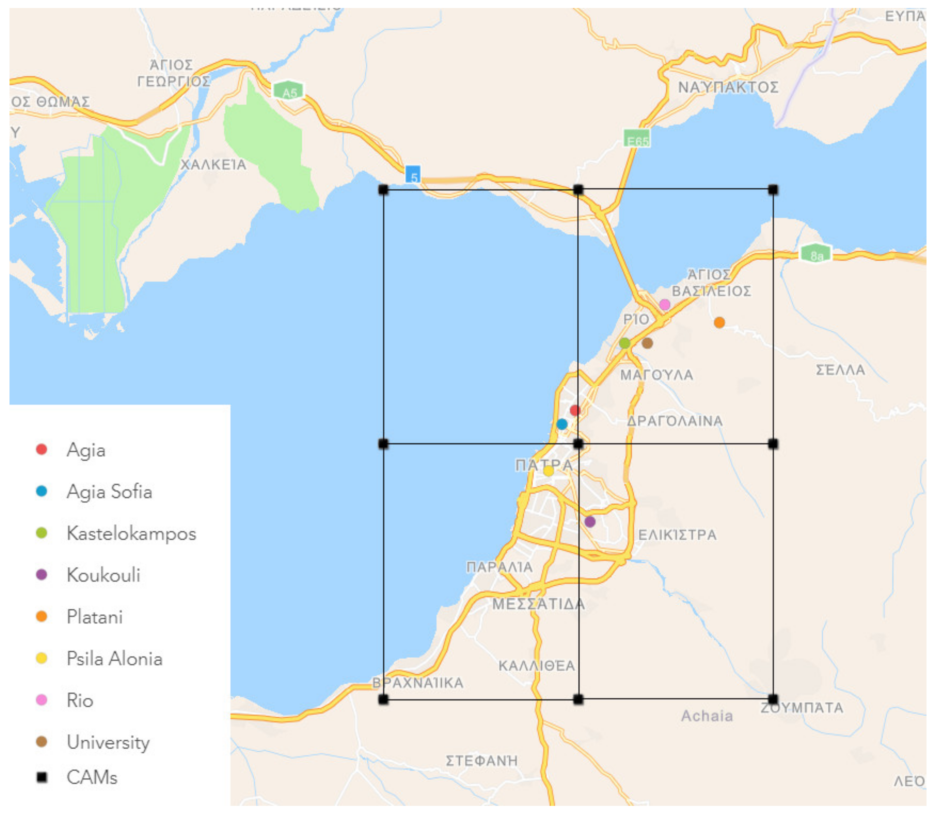
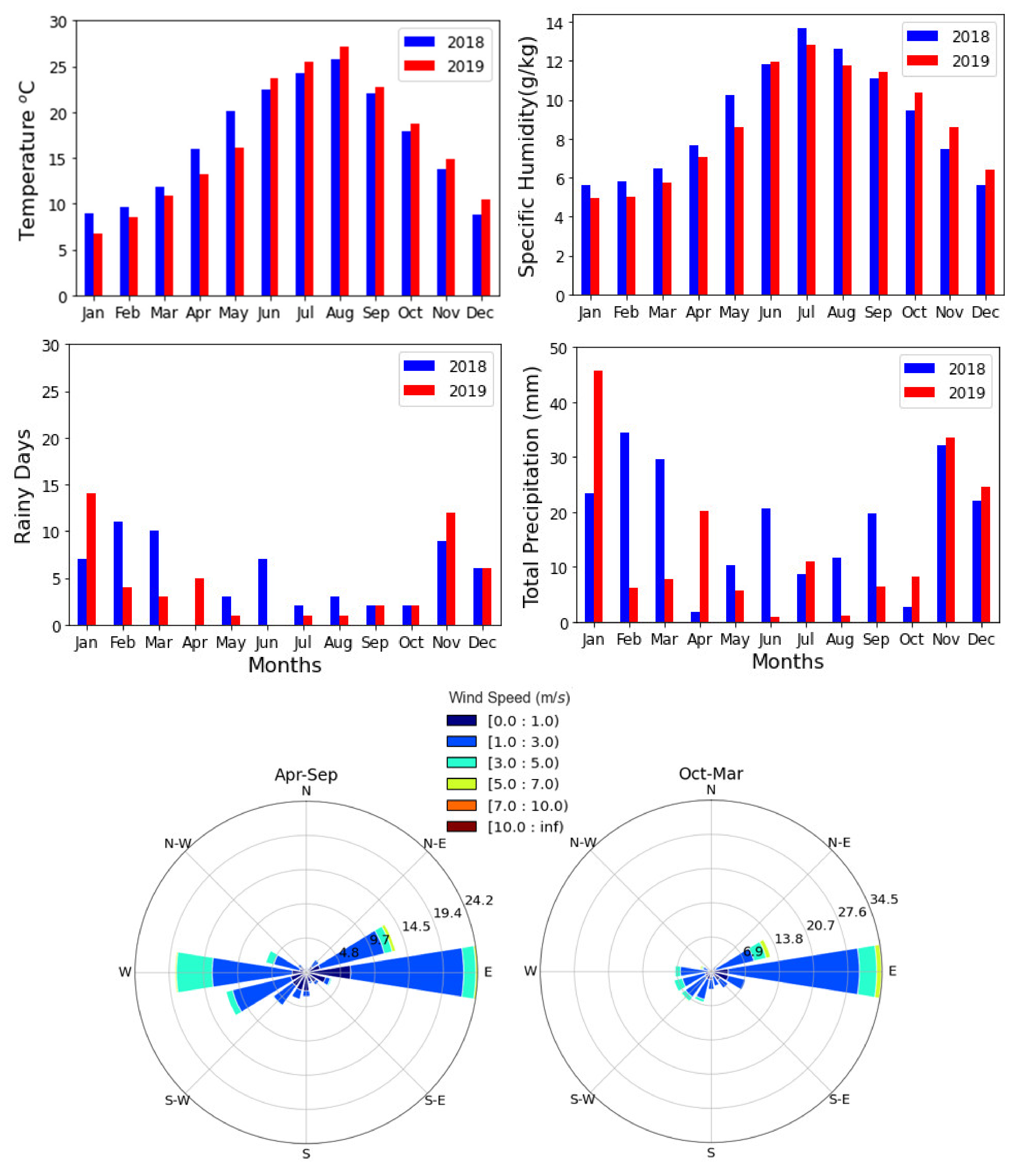
2.1. Investigation Area and Pollution Data

The examined urban area lies between the Mount Panachaikon to the east and the Gulf of Patras to the west. It is a major urban center and has one of the largest ports in Greece, an important channel of communication with Western Europe. The main sources of anthropogenic particulate matter are traffic (road, maritime) and indoor activities (including wood burning, cooking, etc.). According to the Köppen Climate Classification, the area has a Mediterranean climate with a moderate temperature range, warm dry summers and mild wet winters.

Data of PM concentrations (μg/m³ PM_2.5 & PM₁₀) for the municipality of Patras were collected for the period January 2018 to December 2019. Hourly measurements of PM concentrations are received from the Patras Air network, an air quality monitoring system by the laboratory of Atmospheric Physics, University of Patras, that consists of low-cost sensors (Purple Air) measuring the concentration of particulate matter at a dense network of stations installed in Patras. Their performance has been evaluated and calibrations have been derived for Patras [27]. Stations with at least 75% annual data are included in the study and classified considering the location and the dominant emission source. The locations of the stations are illustrated in Figure 1 and their types are listed in

Table 1. The types of monitoring stations used in the study and their annual PM concentrations.

Station Name	Station Type	PM2.5 (μg/m3) (Annual Average)	PM10 (μg/m3) (Annual Average)
Agia	Urban traffic	8.4	11.3
Agia Sofia	Urban traffic	9.3	12.6
Kastelokampos	Suburban background	8.8	11.3
Koukouli	Urban traffic	9.8	13.2
Platani	Rural	5.7	7.8
Psila Alonia	Urban traffic	10.1	13.3
Rio	Suburban background	8.3	11.6
Univ of Patras	Suburban background	6.3	8.6

. Traffic stations are located near roads, whereas to monitor pollution levels in areas less dominated by emission densities, stations are installed in suburban areas. Background stations are located at a certain distance from the area of the highest air pollution emissions and they are influenced by an integrated contribution from sources of pollutants.

CAMS forecasts of PM_2.5 and PM₁₀ concentrations are obtained on a six-hour basis in a 0.1° (~10 km) horizontal resolution (Figure 1). The forecasts are pin-pointed to the location of the air quality monitoring stations using inverse distance weighting [29]. Considering that the weights diminish as a function of distance, the closest points have more influence on the target value [30].

Air pollutant concentrations are affected by the atmospheric conditions prevailing in an area, besides emissions. Temperature affects fuel usage (emissions) and chemical transformations in the atmosphere while precipitation leads to wet deposition and removal of the air pollutants from the atmosphere [31]. Because of the hygroscopic growth of particles, they tend to absorb large amounts of moisture, leading potentially to dry deposition through gravitational settling [32,33,34]. High wind speed contributes to the advection of PM, but in some cases, the topography of an area can impede the transport of air pollutants to the other regions [35]. Figure 2 illustrates the mean monthly values of temperature, rainfall, rainy days, humidity and wind during the study period in the study area, retrieved from the era 5 reanalysis of ECMWF. The 1st semester of 2018 is warmer and more humid compared to 2019, while the opposite is true for the 2nd semester. The number of rainy days (and total precipitation) in January 2019 is double compared to January 2018, affecting the wet deposition of pollutants. In February and March, the situation is reversed, with larger differences between the two years. Prevailing wind direction is from the west and east in the warm season (April to September), transporting marine aerosol particles in the study area, and from the east in the period from October to March.

2.2. Algorithms

2.2.1. Analogue Ensemble

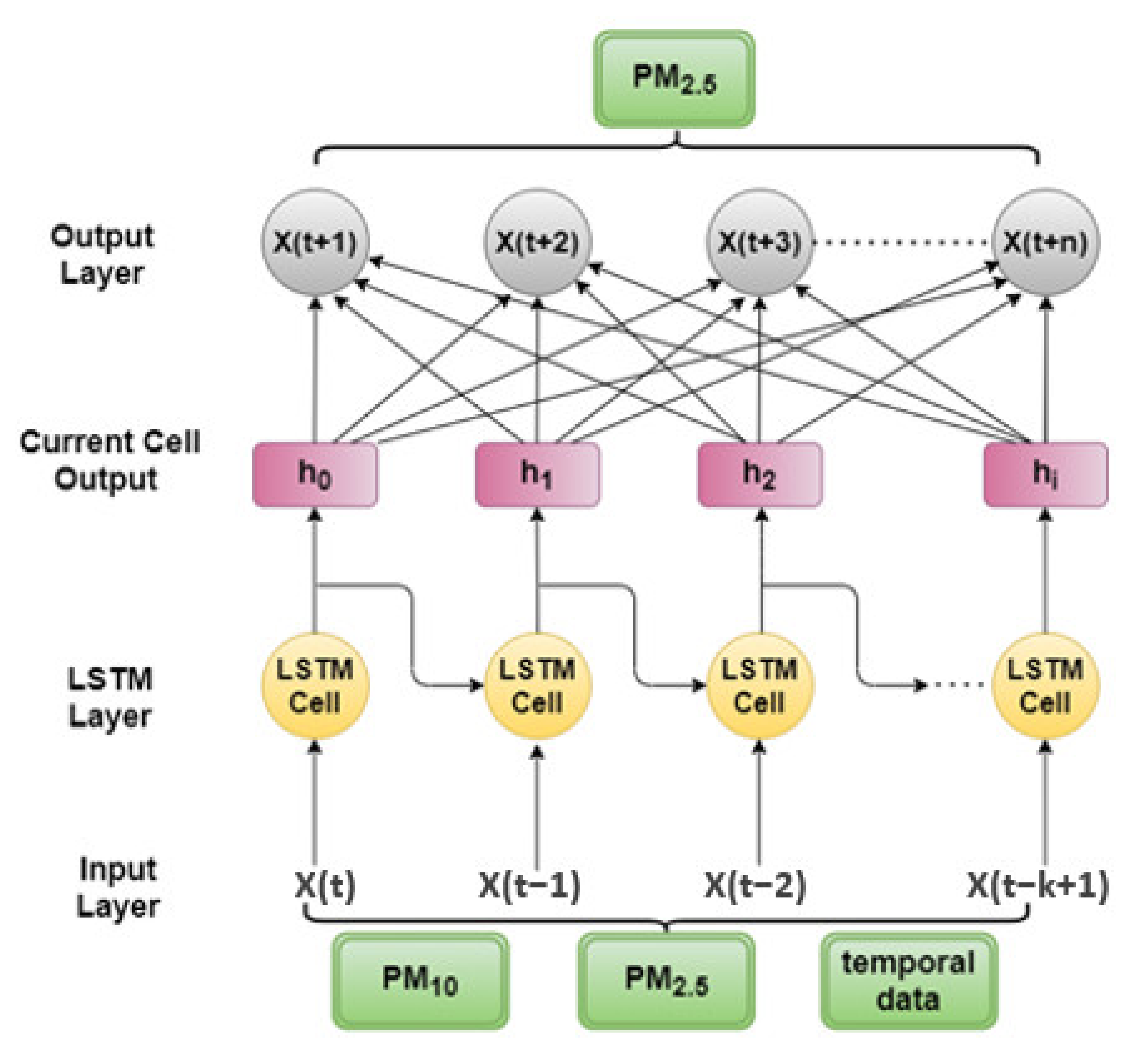
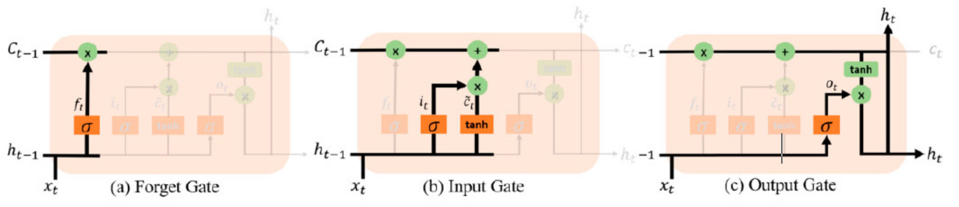
The Analog Ensemble (AnEn) is a dynamic statistical technique that uses time series of past deterministic numerical weather predictions (NWP), and their corresponding observations, to generate a short-term probabilistic forecast for the predictand variable. More concretely, this technique based on the current deterministic forecast selects the most similar historical forecasts to it, from an archive of predictions issued from the same NWP model, and uses the mean value of their corresponding observations as the current AnEn forecast [22]. The probability distribution of the future observation, y, at a given time and location, is P(y|xf), where x, f are the repositories of past observed and predicted values, respectively. The metric used to estimate the similarity between the current deterministic forecast and past predictions was proposed by Delle Monache et al. [16,19]:

$$\left|\left|F_t,A_t\right|\right|={\displaystyle \sum }_{i=1}^{N_v}\frac{w_i}{{\sigma }_{fi}}\sqrt{{\displaystyle \sum }_{j=-\tilde{t}}^{ \tilde{t}}{(F_{i,t+j}-A_{i,t+j})}^2}$$

(1)

where F_t, A_t are the current and analog (historical) NWP deterministic forecasts, respectively, at a certain station for the same forecast lead time t; N_v are the predictor variables, and w_i their assigned weights; the σ_fi is the standard deviation of the past forecasts of each predictor variable at the same station; $\tilde{t}$ is equal to half of the window of the time where the metric is computed; and therefore, F_i,t+j, A_i,t+j are the current and analog forecasts in this time window [19,36,37].

The metric ranks the similarity of past forecasts to the current. For each lead time, the n most similar analogs are chosen from past dates within the training period, and their contemporary observations are the members used to generate the ensemble prediction. The selection of the optimum number of analogs results from computing the Root Mean Squared Error as a function of the number of analogs on the training data set [37,38]. The appropriate ensemble size minimizes the RMSE values between observations and the analog ensemble predictions. From all possible combinations produced by the predictor variables Nv, the combination leading to the lowest RMSE of the AnEn mean is chosen and preserved as constant over the testing period. For each station and forecast lead time, the optimal number of analog members, and the suitable combination of predictors of the target output, are selected.

The Analog Ensemble (AnEn) has been applied in many fields such as renewable energy [36,37,39,40] and meteorology (wind 2 m temperature) [16,19,38,39], and it successfully generates probabilistic forecasts of air quality, and especially predictions of PM_2.5 and PM₁₀ [20,21,41].

2.2.2. LSTM

Air pollutant concentration at a specific time t is influenced not only by the current conditions, but also by the values at a previous time t. Given this, a recurrent neural network (RNN) is selected, which can generate forecasts with sequential information flow [42]. RNN networks are feed-forward neural networks with cyclic connections between neurons that allow one to transfer information, introducing the output from the previous steps as input for the next step. They also have an internal memory in each hidden layer, which retains the interdependency of the data and enable them to preserve long-term information. These models link the previous information with the current target, but when the gap is increased between them, RNNs encounter problems in learning to connect the information. In addition, due to the long-term dependencies, the gradient descent used to determine the weights of the network tends to vanish or explode [43]. To address these problems, LSTM networks were proposed [25]; they are specifically designed to learn dependencies between long-distance information. LSTMs have the structure of a chain of repeating modules of a neural network, like all RNNs, but their repeating modules have a more complex structure [44]. The models consist of an Input Layer, LSTM layers, Dense Layer, and an Output Layer. In the Input Layer, sequential data are created and fed to the LSTM layer, where each LSTM module accepts as input the output of the previous cell as shown in Figure 3.

An LSTM module has a cell state and three gates (namely, forget, input, output). The gates are internal mechanisms of the LSTM cell (Figure 3) that can determine the removal or the addition of information to the cell state. The subscript t denotes the time step in the current moment, so x_t is the input vector to the LSTM unit; h_t−1 is the output vector of the previous cell, of which the memory is represented by c_t−1; h_t c_t, concern the current cell state and will be used in the next cell, ensuring the sequential dependency. W is the weight matrix adjusted for the current input state in each gate and b the vector of the bias terms of the sigmoid layer of neurons.

Initially, the first gate of the LSTM module (Figure 4a), the forget gate, determines what information from the previous cell and to which extent needs to be discarded from it or to be retained in the new cell state. The concatenation of the output from previous cell h_t−1 with the input of current cell x(t) are introduced into the forget gate layer, f_t (Equation (3)), where a sigmoid function (Equation (2)) ranks the output between 0 (complete discarding) and 1 (complete inclusion of information in the new cell) for each value in the cell state C_t−1. In the next step, the new values pass into the input gate (Figure 4b), where a sigmoid layer (Equation (4)) decides if they will be updated, while a hyperbolic tangent function generates a vector of candidate values (Equation (5)). The updated cell is the sum of the previous cell state scaled by f_t, and the new cell state scaled by the input gate i_t (Equation (6)). Finally, the cell state is put into the output gate (Figure 4c), where a sigmoid layer selects the information will be updated (Equation (7)). Then, to produce the cell output h_t, the cell state is activated by a hyperbolic tangent function and multiplied by the result of the output gate o_t (Equation (8)).

$$\sigma \left(t\right)=\frac{1}{1+e^{-t}}$$

(2)

$$f_t=\sigma (W_{f }. \left[h_{t-1},x_t\right]+b_f)$$

(3)

$$i_t=\sigma (W_{i }. \left[h_{t-1},x_t\right]+b_i)$$

(4)

$${\tilde{C}}_t=tanh(W_{C }. \left[h_{t-1},x_t\right]+b_C)$$

(5)

$$C_t=f_t*C_{t-1}+i_t* \tilde{C}$$

(6)

$$o_t=\sigma \left(W_{o }. \left[h_{t-1},x_t\right]+b_o\right)$$

(7)

$$h_t=o_t*\tan \mathrm{h}\left(C_t\right)$$

(8)

LSTM models are considered the most suitable for an air pollution forecast, since the output sequence is a function of the observations in previous steps from multiple different parameters, including the predicted variable. They have been applied to prediction problems of major air pollutants (CO, NO₂, SO₂, PM_2.5, PM₁₀, O₃) [45], while most of them focus on short-term and long-term predictions of PM (PM_2.5, PM₁₀) [46,47,48].

2.3. Predictor Variables

The core predictor variables in the models (AnEn, LSTM) are the CAMS concentrations of PM_2.5 and PM₁₀. Two additional variables are included which serve as proxy to the emissions variability. Julian day is selected to reproduce the variations of emissions associated with processes in the seasonal cycle. Correspondingly, the day of the week is added to the predictor variables to capture the variability of city activities, contributing to air pollutant concentrations.

2.4. Verification Methodology

Statistical indices such as Mean Bias Error (MBE) and Root Mean Square Error (RMSE) [49,50] are used to reflect the error between actual and predicted time series of PM. The MBE defines the systematic error of a model to over or underpredict the observations while the RMSE describes the overall deviation between estimated actual values. The metrics are presented in Equations (9) and (10):

$$\mathrm{MBE}={{\displaystyle \sum }}_{i=1}^n\frac{1}{n}(O_i-F_i)$$

(9)

$$\mathrm{RMSE}=\sqrt{{{\displaystyle \sum }}_{i=1}^n\frac{1}{n}{(O_i-F_i)}^2}$$

(10)

O_i and F_i indicate the observed and forecasted values, respectively. In addition, Taylor plots [51] and soccer plots are used to summarize model performance at each season and station.

Apart from the continuous evaluation described above, categorical statistics are used to quantify the performance of AnEn and LSTM in forecasting extreme levels of PM_2.5 and PM₁₀. The analysis is assessed with the following statistical parameters [50]: (a) the probability of detection (POD), which corresponds to the ratio of the observations forecasted correctly by the method; (b) the false alarm ratio (FAR), representing the proportion of events which are categorized incorrectly as extremes events; (c) the miss mate (MIS), which is a complement score of POD and indicates the extreme events that are not forecasted; (d) the critical success index (CSI) that gives the overall skill of a model to detect correctly an extreme event, in consideration of both false alarms and misses. The statistical range of the above indices is from 0 to 1, with the value of zero indicating the perfect skill for FAR and MIS, whereas for POD and CSI, the unitary value is the ideal situation.

3. Results and Discussion

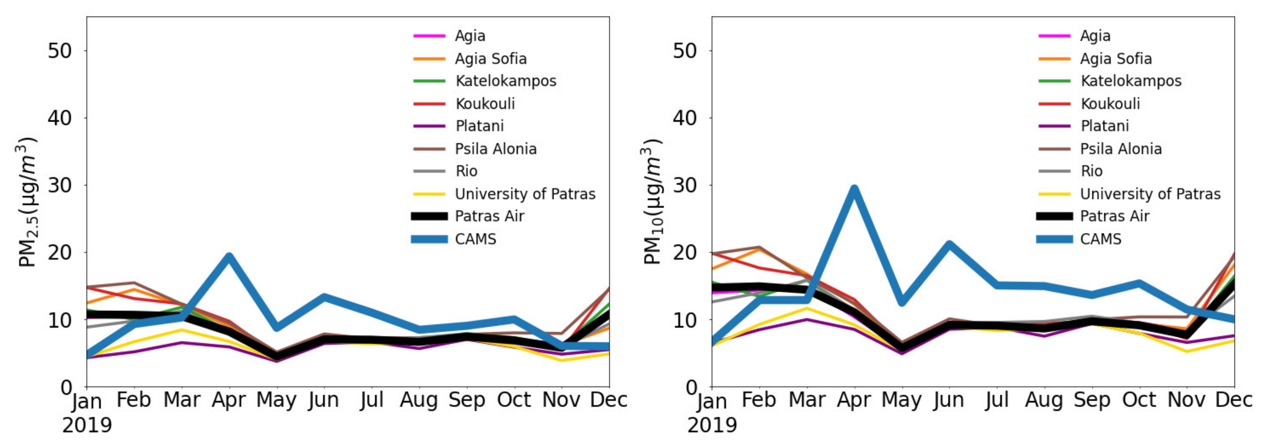
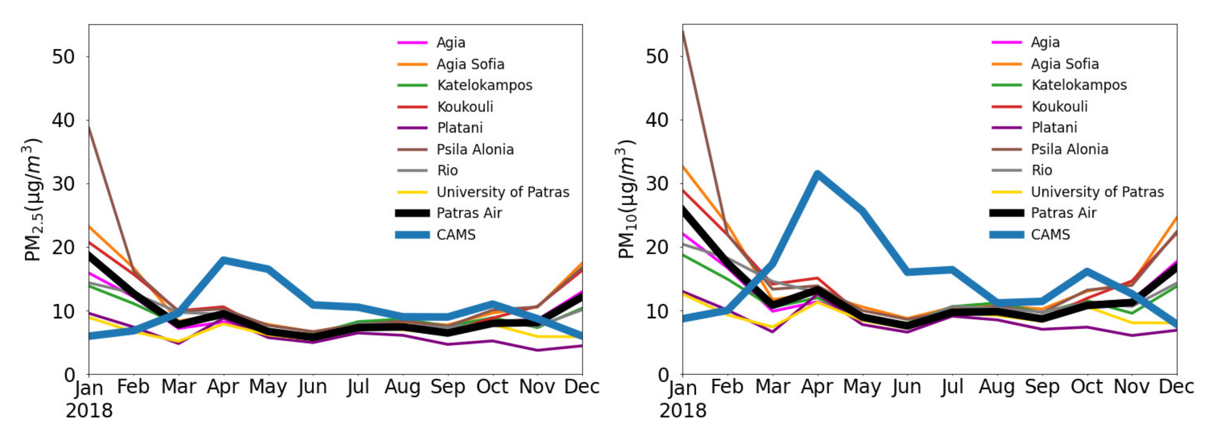
3.1. Observed PM Concentrations

The mean monthly PM₁₀ and PM_2.5 concentrations at each station during 2018–2019 are illustrated in Figure 5. During winter (DJF), the PM levels peak and exhibit the largest spread among stations. The higher atmospheric stability limits pollutant re-circulation and each station is mostly affected by the nearby emission sources. This results in more elevated concentrations at the urban stations compared to suburban stations. PM concentrations are generally constant from May to September as well as between different station types during the same period. The magnitude and variability of PM concentrations are generally consistent across the two years, with the only notable difference being the reduced PM levels in January 2019 compared to January 2018. This can be attributed to the meteorological conditions in the study area presented in Section 2.1; the twofold increase in total precipitation and rainy days in January 2019 exhibits a washing effect on PM concentrations.

3.2. CAMS Evaluation

The comparison of the gridded 0.1° × 0.1° CAMS forecasts with the observations at specific locations is performed on equal terms. Specifically, we make use of the cell de-clustering geostatistical approach to estimate the observed PM concentration onto the CAMS grid cell scale. The 0.1° × 0.1° area around the central CAMS grid point (Figure 1) contains six stations. Splitting the CAMS cell into 4 equal 0.05° × 0.05° boxes, we find either 1 (SE and SW) or 2 (NE and NW) monitoring stations within each box. The observed PM concentration at the CAMS spatial scale is calculated from the weighted sum of the sensor’s concentration, giving weight 0.25 to the stations located in the south and 0.125 to the north stations.

Figure 5 presents the mean monthly PM levels of the central grid point of CAMS shown in Figure 1 against the weighted mean value of the six stations found in its grid. A substantial underestimation occurs during the winter (DJF) while overestimation is evident for the other months. The maximum difference between forecasts and observations is found in January (MB < 0) and April (MB > 0). The most profound reason for this inconsistency by a factor of 2 in DJF is possibly due to errors in the CAMS anthropogenic emissions and especially wood burning, which represents roughly 43% of particulate emissions in the area during winter (Pandis S, personal communication). On the other side, the April overestimation by a factor of ~3 in PM₁₀ in both years is linked to occurred events of Sahara dust transport (17–19/4/18, 12/4/19, 24–28/4/19), not identifiable from the low-cost sensors.

3.3. Development of AnEn and LSTM Models

LSTM and AnEn methods are employed to produce PM₁₀ and PM_2.5 forecasts for the next 90 h at six-hour increments, for the eight air quality monitoring stations located in the urban area of Patras. The datasets of all the stations are separated into two parts, one for training the models (2018) and the other for evaluating them (2019). In this section, we present the implemented configuration of each algorithm issued during the training phase.

3.3.1. AnΕn

Given a forecast, the AnEn algorithm searches similar past forecasts in the training dataset, as described in Section 2.2.1. The selection of the number of analogs and the combination of predictors contribute significantly to the optimal configuration of the AnEn method. Those factors are determined by the leave-one-out cross-validation method in the training dataset (2018) applied for each day. PM₁₀ and PM_2.5 are the target variables. The predictor variables for PM₁₀ (PM_2.5) are four: the same variable provided from the CAMS forecast and three auxiliary variables, namely, the CAMS forecast of PM_2.5 (PM₁₀), the Julian day and the day of week. Seven combinations are produced by the set of the three auxiliary variables, which, with the addition of the AnEn that hasn’t any auxiliary variable, produce a total of eight combinations. For each station, the number of analogs and the variable combination yielding the lowest RMSE between the observed values and the analog ensemble predictions in the train period are identified. The same configuration will be applied in the next section, in the ‘blind’ dataset of the validation period.

Table 2. The optimum configuration of the analog ensemble at each monitoring site with respect to the number of analogs and the subset of auxiliary variables.

	PM2.5					PM10
Station	Optimum Number of Analogs	PM10	JDAY	WDAY	RMSE	Optimum Number of Analogs	PM2.5	JDAY	WDAY	RMSE
Agia	24		X		4.8	18	X	X		6.9
Agia Sofia	12	Χ	Χ	Χ	6.7	11	Χ	Χ	Χ	10
Kastelokampos	24		X		5.7	16	X	X		8
Koukouli	30		X		7.5	22	X	X		10.6
Platani	29		X	X	3.1	24	X		X	4.8
Psila Alonia	21		Χ	Χ	7.2	12	X	Χ		9.9
Rio	27		Χ		4.8	24	X	Χ		7
Univ of Patras	26	X			3.1	30	X	X		4.4
Frequency (%)		25	88	38			100	88	25

displays the optimum configuration per station, i.e., the number of analogs and the combination of predictor variables yielding the minimum RMSE. At most stations, more than 20 analogs are needed to derive the analog forecast for PM_2.5 while fewer members (on average 6 less) are required for PM₁₀ forecasts. In producing PM₁₀ predictions, PM_2.5 is used from all stations while the contrary is generally not true, occurring only at 25% of the stations. For both pollutants, AnEn utilizes as input the Julian day at most stations (seven out of the eight) while WDAY was found important at 2–3 stations only. Hence, the AnEn PM₁₀ forecast relies mostly on three inputs (CAMS forecasts of PM₁₀ and PM_2.5, Julian day) while the AnEn PM_2.5 forecast has two dominant inputs (CAMS forecast of PM_2.5, Julian day). This partly explains the need for fewer analogs for PM₁₀. Adjusting weights to the predictors does not led to better results because they are proven statistically insignificant.

3.3.2. LSTM

Achieving the best performance for the LSTM model is a complex and time-consuming procedure. It is not enough to optimize the hyperparameters of the model; the best combination of them should also be found. In order to construct the architecture of the LSTM network, hyperparameters like the number of hidden layers and nodes in each layer are used, while epoch and batch size, optimizer, loss and activation function should also be employed. A range of values is tested for adjusting each parameter. Through a grid search, numerous trials with all the possible parameter combinations are conducted to result in the final network. As input variables, the same are used as those of AnEn, i.e., observations and CAMS forecasts of PM₁₀ and PM_2.5, the Julian day and the day of week. The data for 2018 of each station are divided into groups of four days, using the first three days of each group as a training set and the fourth day as a validation set to tune the hyperparameters of the model.

The dataset needs preparation before introducing it to the LSTM network, including normalizing the input variables with a range of 0–1 and transforming it suitably for a supervised learning problem. Investigating the correlation between the current target value and its own historical lagged values through the partial autocorrelation (PACF) function, the higher correlation occurred four steps back (t-24 h). Therefore, the LSTM network is trained with a time lag of four timesteps. Using as input the prior four timesteps of predictors (at time t-24 h), the LSTM model is learning from them to produce PM forecasts for each forecast lead time for the next four days.

Based on trial experiment runs, one LSTM layer is proven suitable for the network to avoid overfitting, Although the number of 100 units in the hidden layer seems to be appropriate for all stations, a different network size s tested to achieve the best result for each station. As a concern, the activation of this layer is selected between the functions of relu, sigmoid, softmax and tanh, with the sigmoid function yielding to the least Mean Square Error. After the LSTM layer, two dense layers are added; the first is a fully connected layer with 50 units that works efficiently to connect the neurons to each layer, with the second dense layer acting as the output layer. The output of the model is one-dimensional and utilizes sigmoid activation to produce better forecasts. The model is trained using the Adam gradient-based optimization technique. The Adam optimizer compared with two other stochastic gradient descent algorithms, Stochastic Gradient Descent (SGD) and RMSProp, achieves the minimum error with the lesser number of epochs. After the selection of the optimizer, the number of epochs and batch size are determined, 50 and 76, respectively. For the validation loss, the function must be minimized through optimization, where common choices are the RMSE and MAE. In this case, the RMSE is proven to be a better option. Many of the mentioned results are in accordance with the findings reported in pertinent studies on air pollution forecasting with LSTM models [52,53,54].

3.4. AnEn & LSTM Forecast Verification (Validation Phazse)

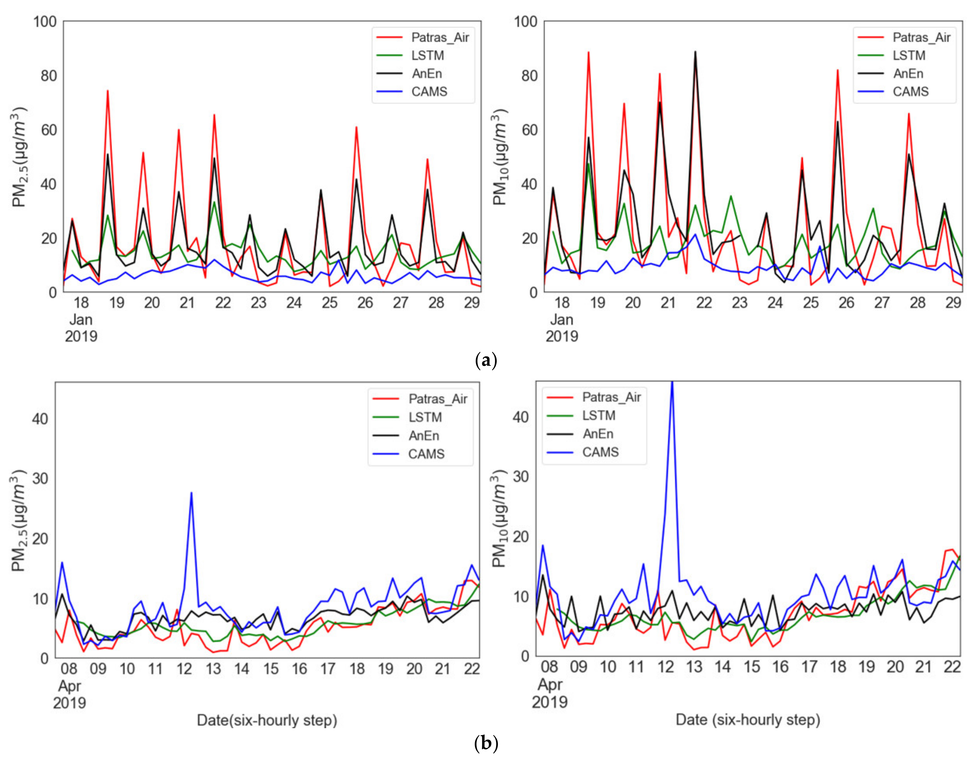
In this section, the optimal configuration of AnEn and LSTM identified during the training phase in the year 2018 (Section 3.3) is applied to the 2019 dataset to evaluate their forecast skill. The verification is carried out for each station separately, covering different forecast lead times, seasons and extreme levels. Verification of CAMS forecasts pin-pointed to the station locations are also used for comparison.

3.4.1. Time Series

Concurrent time series of PM predictions by CAMS, LSTM and AnEn techniques against ground-level observations are produced at six-hour increments for all sites of the study. Figure 6 illustrates the time-series plots of two stations of different types, an urban traffic station (Psila Alonia) and a suburban background station (University of Patras), for a two-week period of January and April 2019, respectively. Those months are selected because, as seen earlier, of the deviation between observations and CAMS peaks during those months. As far as the urban traffic station is concerned (Figure 6a), despite the tendency of CAMS to underestimate PM concentrations conspicuously in January, the AnEn is drastic in correcting the CAMS forecasts towards the magnitude and variability of the measured values. The LSTM captures the variations of the measured values; however, it underestimates the peaks, making it inferior to the AnEn in this type of station. Regarding the background suburban station (Figure 6b), the CAMS model produces quite overestimated forecasts during April. The application of the AnEn in the CAMS forecasts limits to a large extent their distance from the observations. The LSTM, integrating antecedent useful information to the next output, accomplishes a good performance even though it tends to overestimate the minimum. In summary, both the AnEn and the LSTM demonstrate a significant potential to correct the magnitude and phasing of CAMS PM_2.5 and PM₁₀ predictions, with AnEn displaying higher forecast skill at the occasional observed extreme PM concentrations.

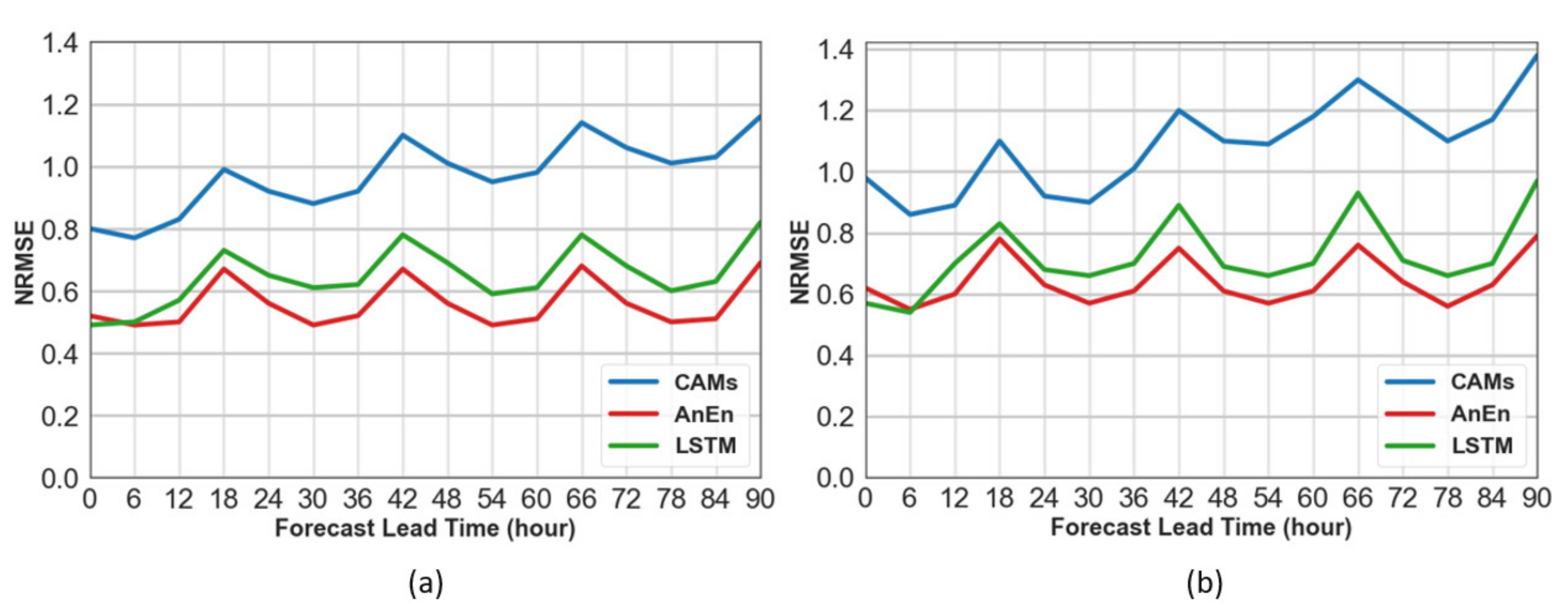
3.4.2. Degradation of Forecast Skill

The verification of the daily cycle of the models has been carried out for horizons up to 90 h ahead, at the eight air quality monitoring stations. Figure 7 displays the normalized RMSE as a function of the forecast lead time from hour 0 to 90 for the PM_2.5 and PM₁₀ levels. The improvements over CAMS are significant at all stations for each forecast lead time. The AnEn generates better results than the LSTM method. The peak error in both approaches is observed at 18 h UTC due to the elevated levels of PM at the specific evening rush time. Moreover, the degradation of the forecast skill as the forecast interval increases is milder for the corrected schemes, being slowest for AnEn (0.015 increase in NRMSE per forecast day) compared to LSTM (0.043 per day) and CAMS (0.079 per day).

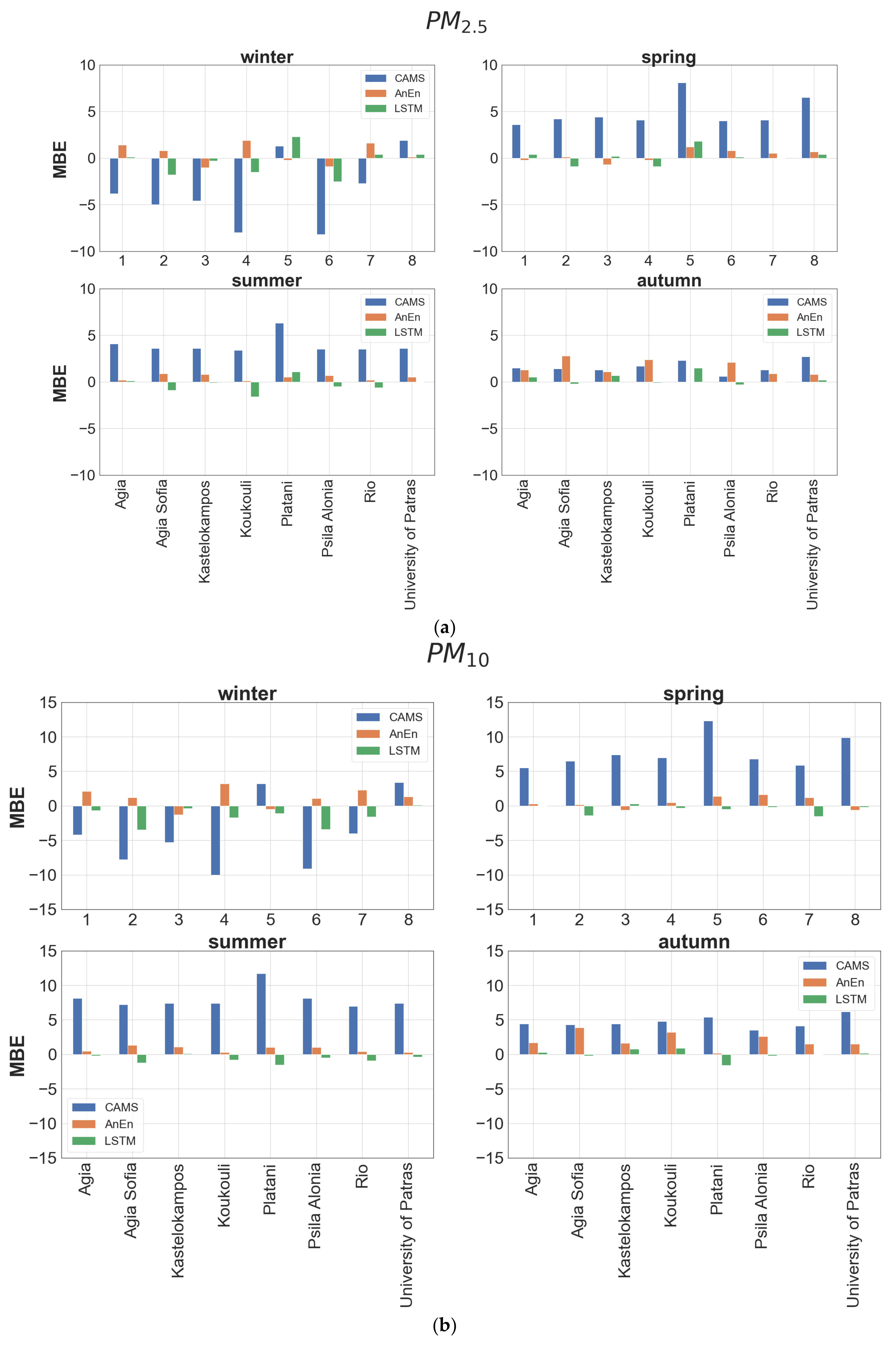
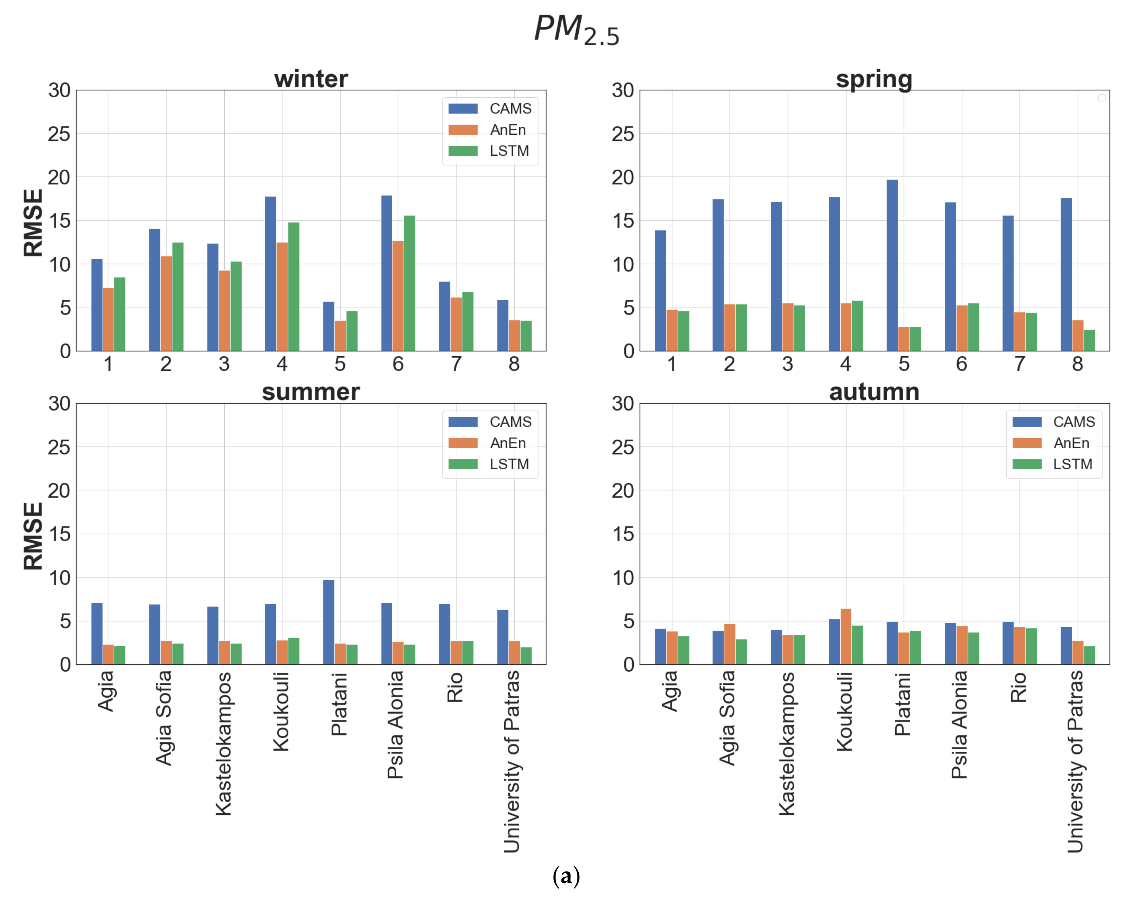
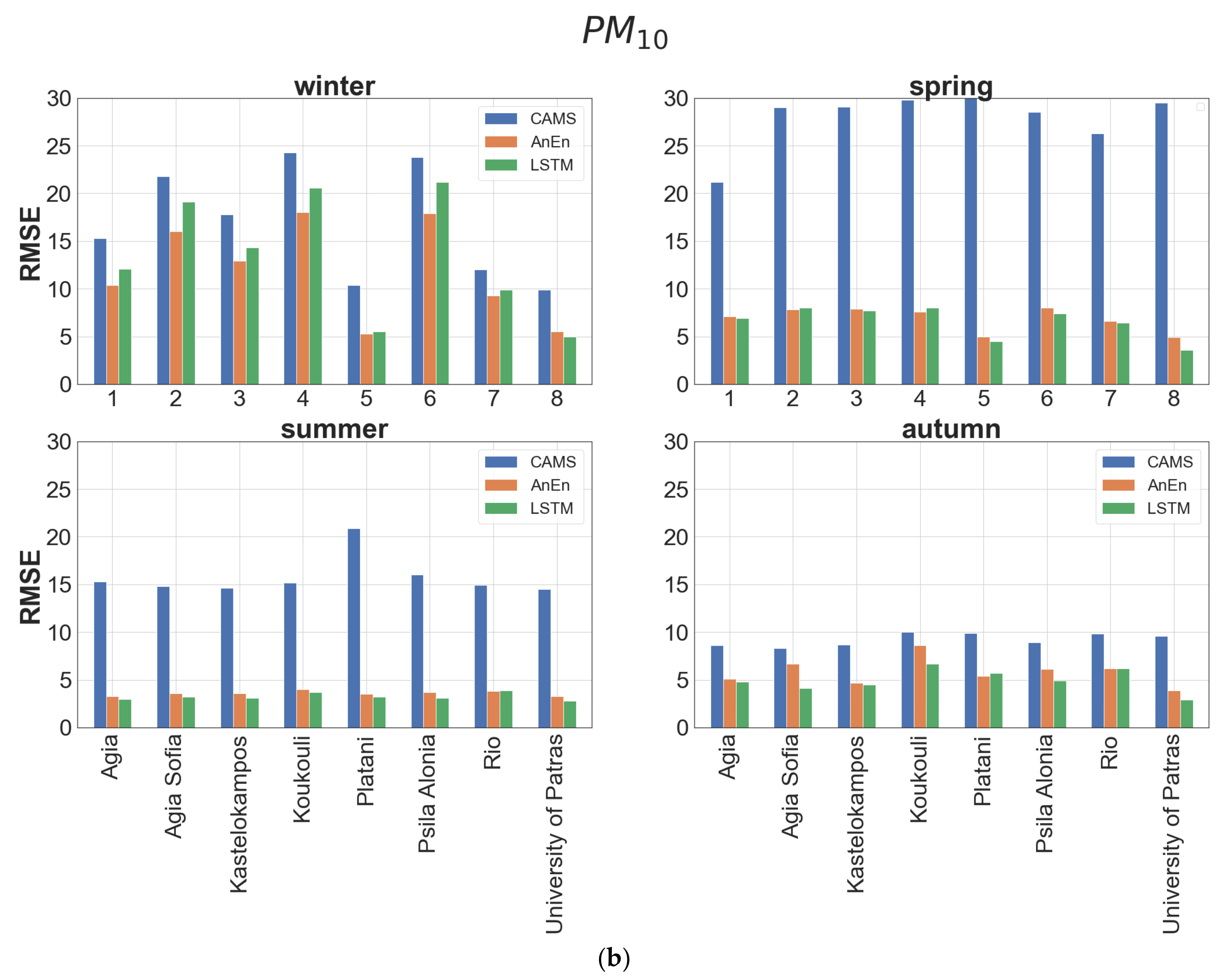
3.4.3. Error Indices

Typical error metrics, such as MBE and RMSE, are calculated at each monitoring station in annual, seasonal and monthly temporal scales to gain insight on the forecast skill of each model. On an annual scale, CAMS shows positive bias for both pollutants, with the MBE of PM₁₀ being roughly double compared to PM_2.5 (

Table 3. MBE of PM_2.5 and PM₁₀ for forecasts of CAMS, AnEn and LSTM at each station.

	PM2.5			PM10
STATION	CAMs	AnEn	LSTM	CAMs	AnEn	LSTM
Agia	1.5	0.7	0.3	3.8	1.1	−0.1
Agia Sofia	1.7	1.1	−0.9	3.6	1.7	−1.4
Kastelokampos	1.4	0.1	0.1	3.9	0.2	0.2
Koukouli	0.6	1.0	−1.1	2.7	1.7	−0.5
Platani	4.6	0.4	1.7	8.2	0.6	−1.1
Psila Alonia	0.2	0.7	−0.8	2.9	1.6	−1.0
Rio	1.8	0.7	−0.1	3.7	1.3	−1.0
University of Patras	3.9	0.6	0.2	7.0	0.5	0.1
Average (absolute)	2.0	0.7	0.7	4.5	1.1	0.7

). As illustrated in Figure 8, the annual overestimation from CAMs is found for all seasons except for winter, when quite underestimated forecasts are distinguishable. The annual biases of both approaches are smaller than 1 μg/m⁻³ in absolute terms when aggregated over all stations, being reduced compared to CAMS by a factor of at least 3 (Table 3). The AnEn technique reduces the bias of CAMS forecasts by approximately 65%, in absolute terms. On the annual scale, it generates predictions with a slight overestimation, in the range 0.1 to 1.1 μg/m⁻³ for PM_2.5 and 0.2 to 1.7 μg/m⁻³ for PM₁₀. The bias reduction is consistent across all seasons. In contrast to AnEn, the LSTM model exhibits a minor underestimation tendency ranging from −0.9 to 1.7 μg/m⁻³ for PM_2.5 and −1.4 to 0.2 μg/m⁻³ for PM₁₀, which demonstrates slightly underestimated concentrations with small negative MBE values.

The performance of each model is also evaluated using RMSE, a widely used reliability factor where errors of different signs do not compensate as in the case of MBE. As can be inferred from

Table 4. RMSE of PM_2.5 and PM₁₀ for forecasts of CAMS, AnEn and LSTM at each station.

	PM2.5			PM10
Station	CAMS	AnEn	LSTM	CAMS	AnEn	LSTM
Agia	9.3	4.7	5.0	15.4	6.8	7.2
Agia Sofia	11.8	5.9	6.1	20.0	8.8	9.5
Kastelokampos	11.5	5.6	6.0	19.4	7.9	8.3
Koukouli	12.9	6.9	8.1	21.1	10.5	11.3
Platani	12.3	3.3	3.1	21.6	5.0	5.0
Psila Alonia	13.1	7.0	8.1	20.7	10.0	10.9
Rio	9.9	4.5	4.4	17.3	6.6	6.7
University of Patras	10.4	3.1	2.6	18.5	4.4	3.6
Average	11.4	5.1	5.4	19.3	7.5	7.8

, neither method is clearly superior. Both models show a gross annual RMSE value (averaged over all stations) lower by approximately 50% for PM_2.5 and 60% for PM₁₀ with respect to CAMS. The best performance (~75% RMSE improvement) for both models is met at the suburban background stations (University of Patras, Platani) and the worst (~50% RMSE improvement) is noticed at the urban traffic stations (Koukouli, Psila Alonia). AnEn prevails over the LSTM method in urban traffic stations (high PM levels) while the opposite is true at the background stations. According to the seasonal values of RMSE at each station, the AnEn attains better results than LSTM during winter (Figure 9). The largest improvement of AnEn over CAMS forecasts is observed in spring and summer and the minimum in autumn. Generally, in terms of RMSE, AnEn is proven more efficient for predicting periods with high particulate air pollution levels, whereas the LSTM is marginally more successful, in seasons with moderate emissions.

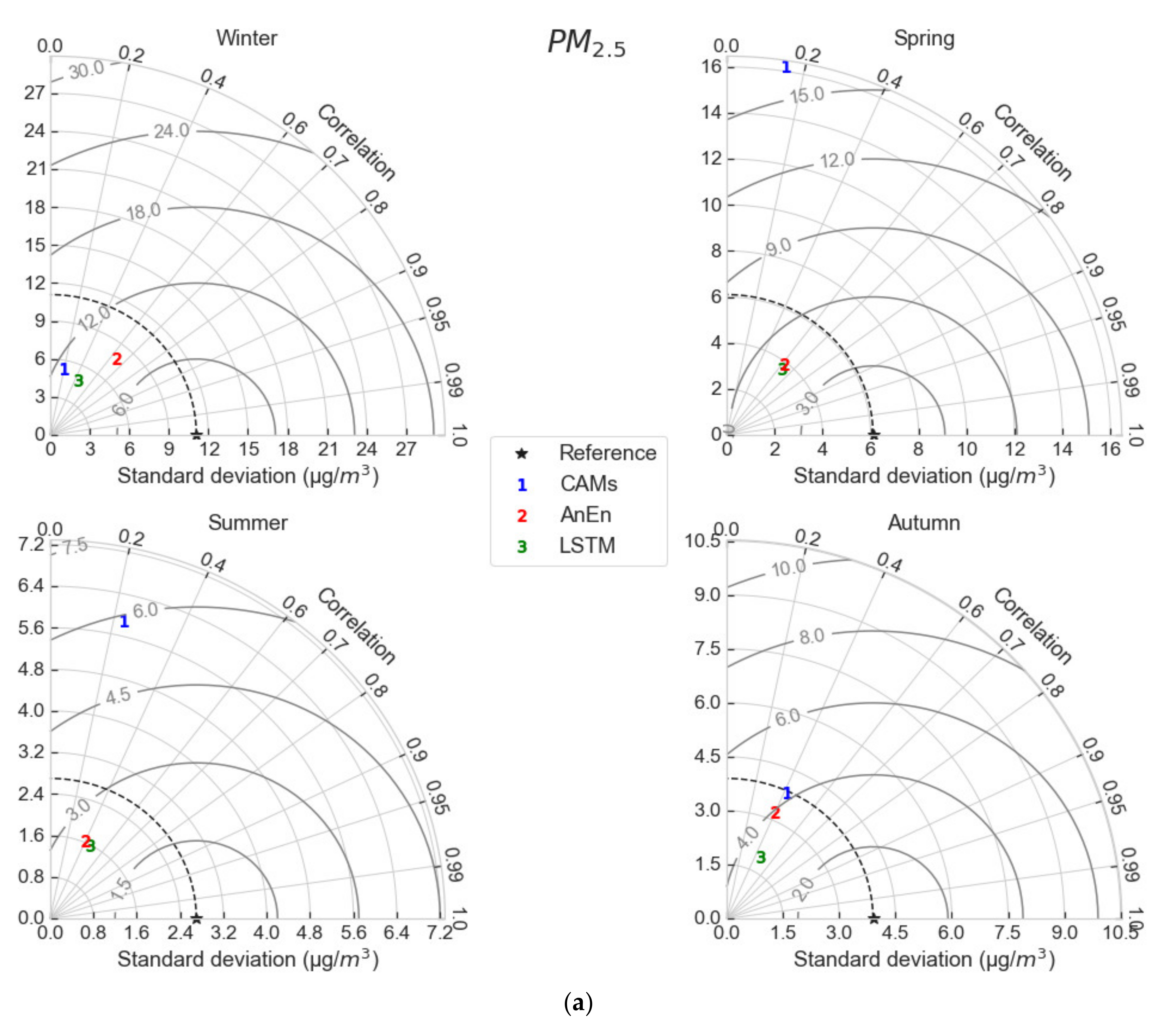
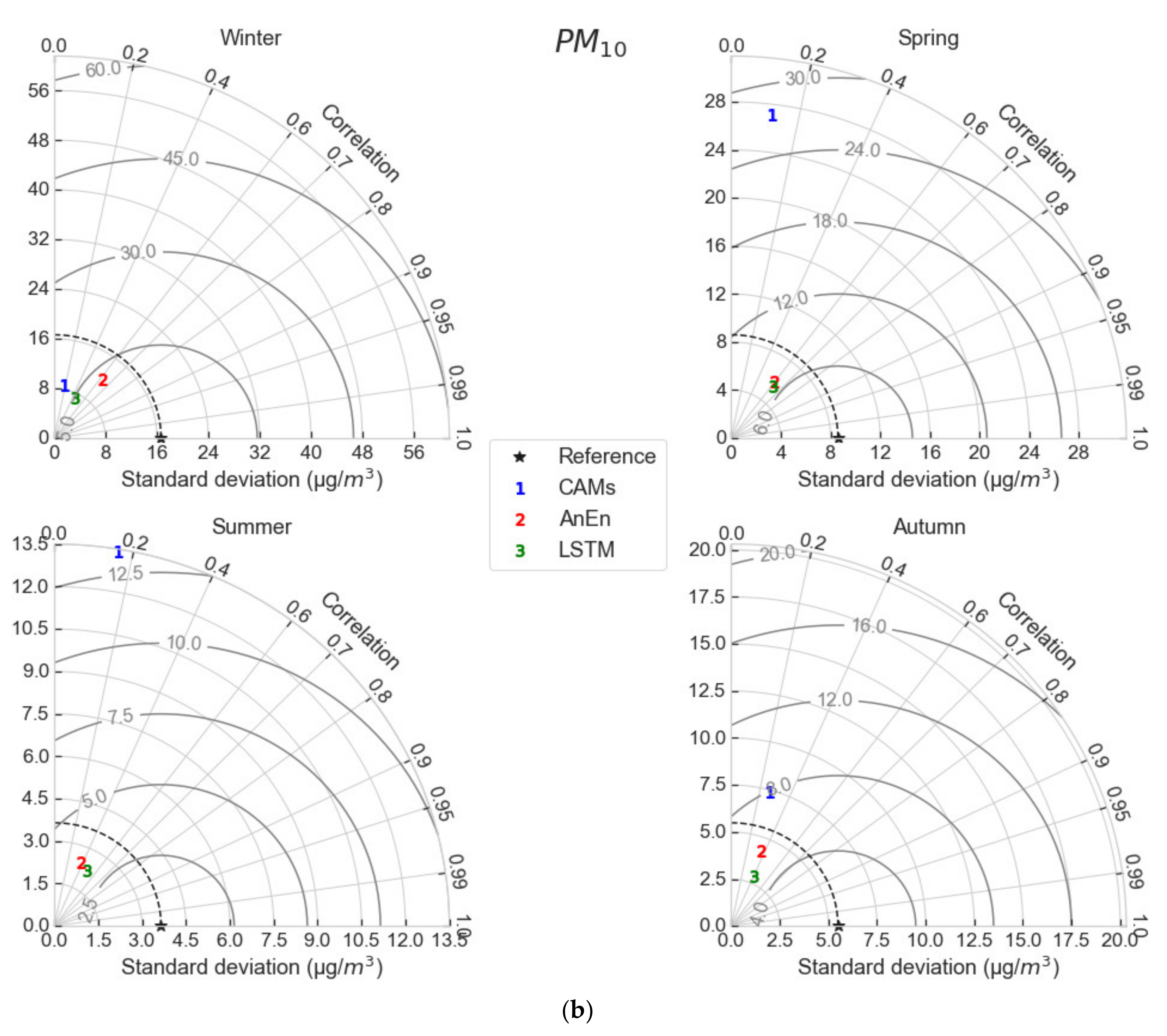
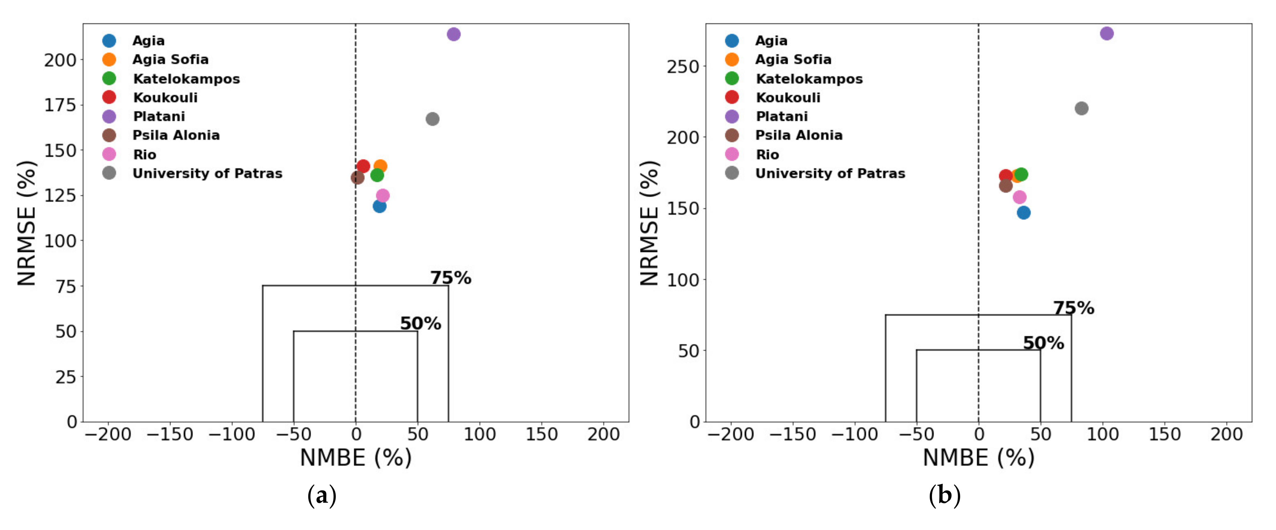
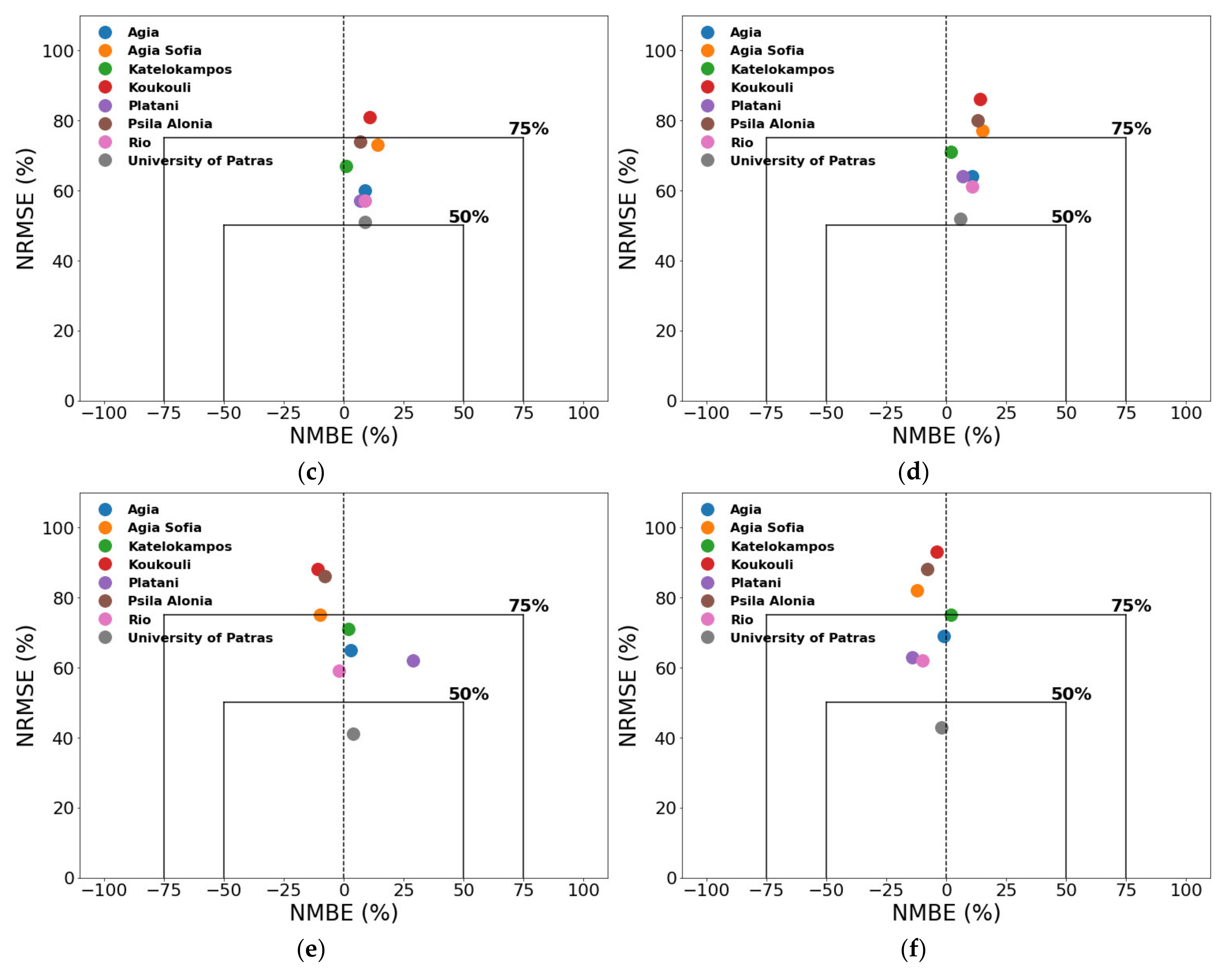
3.4.4. Taylor & Soccer Plots

Taylor diagrams check the prediction skill of models from various angles, summarizing RMSE, Pearson Correlation coefficient (PCC) and standard deviation (STD) in a single plot (Figure 10). The semi-circles in the plots are RMSE contours and the reference point stands for the statistics for the observed field. The values of statistical metrics are derived from the seasonal means of all stations. For PM_2.5 (Figure 11a), CAMS forecasts show the highest combined skill in autumn (PCC ~ 0.4, STD ratio ~ 1) while in winter, the underestimation of the PM concentrations degrades the skill (PCC ~ 0.2, STD ratio ~ 0.5). In summer, CAMS inflates the observed variance by a factor of 2; in spring, the inflation is larger (STD ratio ~ 3), partly explained by the unidentified soiling events from the sensors. In winter, when the highest PM levels are recorded, AnEn clearly outscores LSTM improving noticeably all three validation scores (error, phasing, variance). In autumn, AnEn achieves better variance compared to LSTM at the expense of a larger error, hence, there is no clear winner. Last, in spring and summer, the combined skill of AnEn and LSTM is similar. The results for PM₁₀ (Figure 11b) indicate a similar picture with those of PM_2.5. In summary, the seasonal Taylor diagrams point out the essential improvement of CAMS forecasts in winter through AnEn, which corrects appreciably the CAMS forecasts, achieves clearly smaller RMSE, higher correlation and standard deviation closer to the observed values, than the LSTM.

The visualization of the normalized MBE versus the normalized RMSE of each station by means of soccer plots allows the comparative assessment of model skill across different type of stations. Apart from CAMS (Figure 11) exceeding the border of 75%, the statistical-based models AnEn and LSTM position the stations in a bounded area, with the NMB not going beyond the limits of 20% in any station, and the NRMSE being restricted mostly to under 75%. For AnEn (Figure 11), the overall performance of stations is within the range of 50–75%, with the only exception being the urban traffic station of Koukouli for the PM_2.5. For the PM₁₀, two additional urban stations, those of Agia Sofia and Psila Alonia, are found outside the bigger box. An overestimation bias is evident for both PM_2.5 and PM₁₀ in all stations. For LSTM (Figure 11), the results appear more scattered compared to AnEn. Exceptional model performance is noticed for the suburban station of the University of Patras which exhibits the smaller error, whereas the urban stations of Psila Alonia and Koukouli are outside of the greater box. A slight underprediction bias occurs across all the stations for the PM₁₀ concentrations, apart from the Kastelokampos, which displays an overestimation bias. For the PM_2.5, half of the stations show overestimation. Generally, the skill of the statistical methods for the urban stations are found within the bounds or exceed them, whereas in the suburban or background stations, where lower air pollutant levels prevail, a good performance is achieved.

3.4.5. Extremes

The occurrence of extreme particulate pollution events is rare in the examined region, but of particular importance for human activities. Consequently, it is deemed necessary to evaluate the proposed methods based on their performance in PM exceedances. Regarding the PM concentrations in the specific area, extreme values of PM_2.5 and PM₁₀ are considered those exceeding 20 and 40 μg/m⁻³ [55], respectively. The small representativity of those records in the dataset makes the task of verification more challenging. The capacity of AnEn and LSTM methods and the CAMS estimator in forecasting PM_2.5 and PM₁₀ extreme values is assessed with the statistical scores POD, FAR, CIS and MIS mentioned in Section 2.4 (

Table 5. The probability of detection (POD), false alarm rate (FAR), critical success index (CIS) and miss rate (MIS) from CAMS, AnEn and LSTM for PM_2.5 and PM₁₀.

	POD	FAR	MIS	CSI
PM2.5 ≥ 20
CAMS	0.06	0.95	0.94	0.03
AnEn	0.52	0.46	0.48	0.36
LSTM	0.20	0.42	0.80	0.16
PM10 ≥ 40
CAMS	0.02	0.99	0.98	0.01
AnEn	0.40	0.48	0.60	0.30
LSTM	0.04	0.55	0.96	0.04

). Generally, the indices for CAMS show substantial weakness to capture extreme values. It is considered more constructive to juxtapose mainly the skills of the statistical methods, AnEn and LSTM. Based on the value of the probability of detection (POD) for PM_2.5, the AnEn is superior in detecting the extreme values, giving 0.52 against 0.20 of the LSTM, which means more than half the extreme events are detected by the AnEn. However, the false alarm value for AnEn and LSTM is 0.46 and 0.42, respectively, indicating a considerable proportion of the forecast extreme events which does not occur. The composite index CSI for AnEn is 0.36 and dominates over the LSTM index being 0.16. For PM₁₀, the AnEn generally replicates the PM_2.5 results, achieving a CSI of 0.30 while LSTM fails (CSI = 0.04). The CSI index takes into account hits, false alarms and misses; hence, it constitutes a more reliable statistical measure; so relying on it, we conclude that the AnEn outscored LSTM in identifying extreme values.

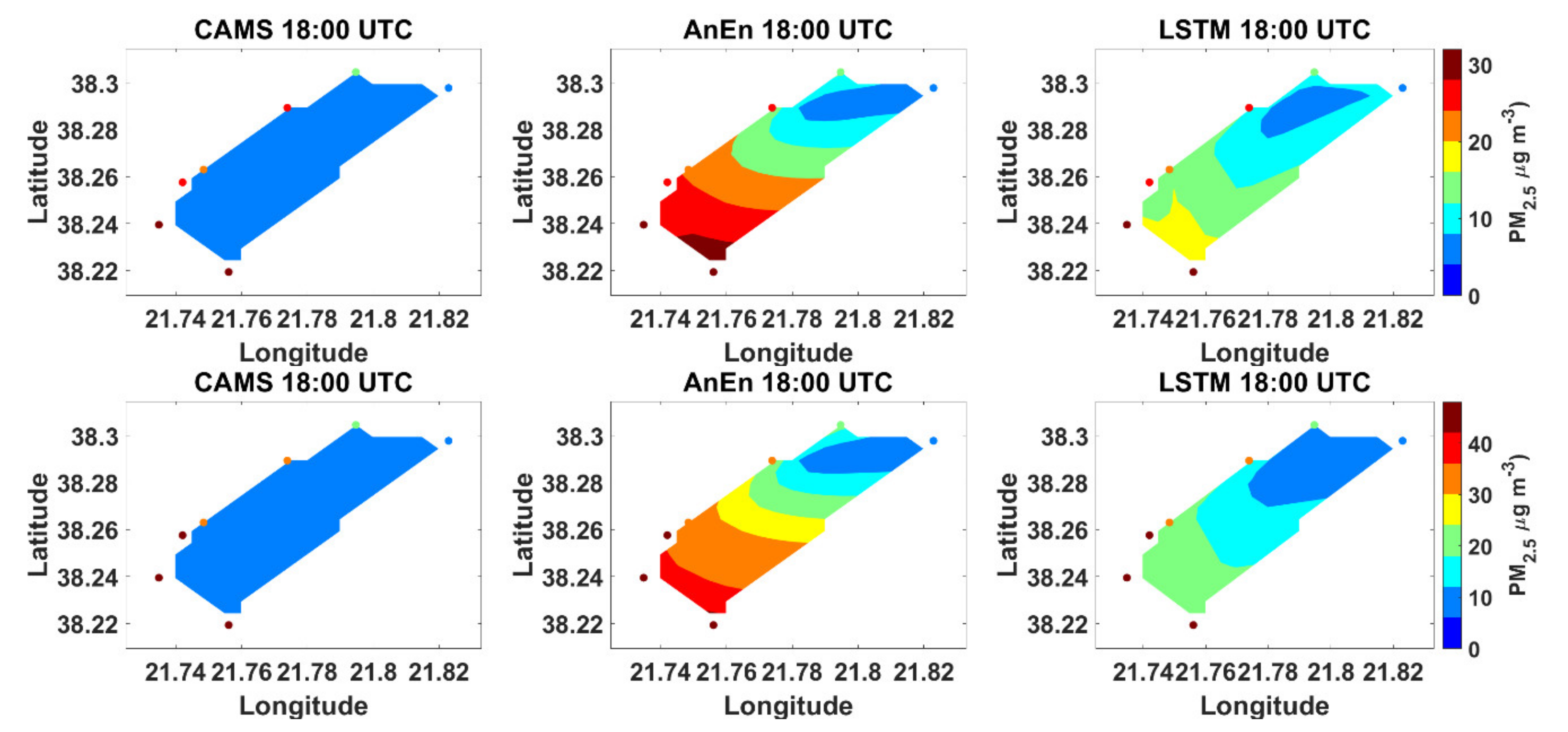
3.4.6. Forecast Maps

In this section, we extend the analysis to two dimensions, and we present forecast maps of air pollution from the investigated techniques. For CAMS, the area enclosed by the stations corresponds to the forecast at the central grid point (Figure 12). For AnEn and LSTM, the maps were generated from triangulation-based natural neighbor interpolation from their corresponding forecasts at each station. As already discussed, CAMS underestimates the average, across all stations, PM_2.5 and PM₁₀ concentrations (Figure 12). AnEn and LSTM improve the predictions at the point locations of the stations, yielding spatial variability. Between them, AnEn reproduces with higher accuracy the observed south-north gradient, mostly due to its better skill at the peak values observed at the southern stations.

4. Conclusions

In this work, we evaluate the CAMS PM forecasts at local scale against in-situ measurements, spanning 2 years, obtained from a network of stations located in an urban coastal Mediterranean city in Greece. Then, we compare the performance of a statistical method (AnEn) and a deep-learning network (LSTM) in forecasting PM₁₀ and PM_2.5 concentrations at station level, using only open data as inputs; namely, the PM observations from a dense network of calibrated low-cost sensors and the corresponding operational CAMS forecasts. The models are trained with the datasets of 2018; the four-day ahead predictions at 6 h increments are validated with the 2019 datasets. Hence, the purpose of the study is two-fold: evaluate CAMS in an urban agglomeration and downscale its forecasts at sub-km scale.

The comparison of the PM_2.5 and PM₁₀ concentrations at the monitoring stations, upscaled at the CAMS grid, show an underestimation of PM_2.5 and PM₁₀ concentrations by a factor of 2 in CAMS forecasts during winter, indicating a misrepresentation of anthropogenic particulate emissions such as wood-burning. Overestimation is evident for the other seasons and CAMS achieves the lower error in autumn.

The AnEn technique seeks analog patterns in an input database. The LSTM technique uses the CAMS forecasts as features to identify the pattern of PM concentration. Both approaches effectively predict PM concentrations, capturing adequately the variations of measured values in all stations and achieving substantial lower error than CAMS forecasts. The AnEn reduces the CAMS RMSE by 55% and 60% for PM_2.5 and PM₁₀, respectively, and shows a good ability to approach the ground-based measurements throughout the year, and its skill is consistent across all pollution levels, including the extreme values. The LSTM exhibits a trend for underestimating the high PM concentrations, making it more suitable for stations and periods with moderate PM levels. LSTM demonstrated difficulty in capturing the exceedances of the limit value of 25 and 40 μg/m³, for PM_2.5 and PM₁₀, respectively. AnEn and LSTM have similar skill in suburban stations, whereas AnEn is proven more efficient in the urban stations which record higher PM levels, especially in winter. Seasonally, the AnEn is superior to the LSTM in winter when the PM concentrations are considerably high. In the other seasons, in particular, spring and summer, the composite skill of both methods is similar. The results were robust up to 4 days ahead forecasts and the corrected predictions demonstrated only a mild degradation. Especially, the predictive skill of AnEn degrades notably more slowly as the forecast interval increases compared to CAMS and LSTM.

The generation of forecast maps demonstrated the superior ability of AnEn to reproduce the observed pollution pattern with a south–north gradient. This supports the statement that its forecasts could constitute a reliable index for a health decision support system in cases where the variability of the fine-scale non-represented processes (e.g., weather, traffic, agricultural burning, sandstorms, industrial activity, etc.) follows consistent sub-daily and sub-seasonal patterns. In the city of Patras, those conditions are highly fulfilled.

AnEn and LSTM techniques are statistical methods tied to the completeness of the training data and the stationarity between the training and testing datasets. For the purposes of the short-term PM forecasting investigated here, the two continuous years dataset was found to meet both requirements. In this setting, both techniques are proven reliable tools for air pollution forecasting, and they could be used in other regions with small modifications. Those include the optimization of the architecture hyperparameters (LSTM: number of hidden layers and nodes, learning rates; AnEn: number of analogs) and the selection of the important inputs. The configuration of LSTM is time-consuming because it demands tuning and testing of all the possible combinations of its hyper-parameters. AnEn has lower computational demands and showed better performance across seasons and pollution levels.

A limitation of the current study is the lack of explicit meteorological and emission predictors in the statistical approaches as such data are not available. This will be implemented in a future experiment using forecasts from the Weather Research and Forecasting model. High-resolution weather forecasts could incorporate information about urban processes not parameterized in this study, such as advection and diffusion, with a view to improving further the PM₁₀ and PM_2.5 prediction in cities at sub-km scale.

References

1. Brauer, M.; Amann, M.; Burnett, R.T.; Cohen, A.; Dentener, F.; Ezzati, M.; Henderson, S.B.; Krzyzanowski, M.; Martin, R.V.; Van Dingenen, R.; et al. Exposure assessment for estimation of the global burden of disease attributable to outdoor air pollution. Env. Sci. Technol. 2012, 46, 652–660. [Google Scholar] [CrossRef] [PubMed] [Green Version]
2. WHO. Review of Evidence on Health Aspects of Air Pollution—REVIHAAP Project: Technical Report; WHO: Copenhagen, Denmark, 2013; p. 302. [Google Scholar]
3. Lelieveld, J.; Evans, J.S.; Fnais, M.; Giannadaki, D.; Pozzer, A. The contribution of outdoor air pollution sources to premature mortality on a global scale. Nature 2015, 525, 367–371. [Google Scholar] [CrossRef] [PubMed]
4. Pope, C.A.; Dockery, D.W.; Schwartz, J. Review of Epidemiological Evidence of Health Effects of Particulate Air Pollution. Inhal. Toxicol. 1995, 7, 1–18. [Google Scholar] [CrossRef]
5. Pope III, C.A.; Burnett, R.T.; Thun, M.J.; Calle, E.E.; Krewski, D.; Ito, K.; Thurston, G.D. Lung Cancer, Cardiopulmonary Mortality, and Long-term Exposure to Fine Particulate Air Pollution. JAMA 2002, 287, 1132–1141. [Google Scholar] [CrossRef] [PubMed] [Green Version]
6. Urch, B.; Brook, J.R.; Wasserstein, D.; Brook, R.D.; Rajagopalan, S.; Corey, P.; Silverman, F. Relative Contributions of PM2.5 Chemical Constituents to Acute Arterial Vasoconstriction in Humans. Inhal. Toxicol. 2014, 16, 345–352. [Google Scholar] [CrossRef] [PubMed]
7. EEA. Air Quality in Europe—2019 Report; EEA Report No 10/2019; European Environment Agency: Copenhagen, Danmark, 2019; Available online: https://www.eea.europa.eu/publications/air-quality-in-europe-2019 (accessed on 20 January 2021).
8. Li, L.; Zhang, J.H.; Qiu, W.Y.; Wang, J.; Fang, Y. An Ensemble Spatiotemporal Model for Predicting PM2.5 Concentrations. Int. J. Environ. Res. Public Health 2017, 14, 549. [Google Scholar] [CrossRef] [PubMed] [Green Version]
9. Salnikov, V.G.; Karatayev, M.A. Impact of air pollution on human health: Focusing on Rudnyi Altay industrial area. Am. J. Environ. Sci. 2011, 7, 286–294. [Google Scholar] [CrossRef]
10. CAMS. Available online: https://atmosphere.copernicus.eu/data (accessed on 28 December 2020).
11. ECMWF. Available online: https://www.ecmwf.int/en/about/media-centre (accessed on 28 December 2020).
12. Kalnay, E. Atmospheric Modelling, Data Assimilation and Predictability; Cambridge University Press: Cambridge, UK, 2003; p. 341. [Google Scholar]
13. Kioutsioukis, I.; Melas, D.; Zerefos, C.; Ziomas, I. Efficient Sensitivity Computations in 3D Air Quality Models. Comput. Phys. Commun. 2005, 167, 23–33. [Google Scholar] [CrossRef]
14. Zhang, Y.; Seigneur, C.; Bocquet, M.; Mallet, V.; Baklanov, A. Real-Time Air Quality Forecasting, Part II: State of the Science, Current Research Needs, and Future Prospects. Atmos. Environ. 2012, 60, 656–676. [Google Scholar] [CrossRef]
15. Borrego, C.; Monteiro, A.; Pay, M.T.; Ribeiro, I.; Miranda, A.I.; Basart, S.; Baldasano, J.M. How bias-correction can improve air quality forecasts over Portugal. Atmos. Environ. 2011, 45, 6629–6641. [Google Scholar] [CrossRef] [Green Version]
16. Delle Monache, L.; Nipen, T.; Liu, Y.; Roux, G.; Stull, R. Kalman filter and analog schemes to postprocess numerical weather predictions. Mon. Weather Rev. 2011, 139, 3554–3570. [Google Scholar] [CrossRef] [Green Version]
17. Kioutsioukis, I.; Galmarini, S. De praeceptis ferendis: Good practice in multi-model ensembles. Atmos. Chem. Phys. 2014, 14, 11791–11815. [Google Scholar] [CrossRef] [Green Version]
18. Kioutsioukis, I.; Im, U.; Solazzo, E.; Bianconi, R.; Badia, A.; Balzarini, A.; Baró, R.; Bellasio, R.; Brunner, D.; Chemel, C.; et al. Insights into the deterministic skill of air quality ensembles from the analysis of AQMEII data. Atmos. Chem. Phys. 2016, 16, 15629–15652. [Google Scholar] [CrossRef] [Green Version]
19. Delle Monache, L.; Eckel, F.A.; Rife, D.L.; Nagarajan, B.; Searight, K. Probabilistic weather prediction with an analog ensemble. Mon. Weather Rev. 2013, 141, 141,3498–516. [Google Scholar] [CrossRef] [Green Version]
20. Delle Monache, L.; Alessandrini, S.; Djalalova, I.; Wilczak, J.; Knievel, J.C.; Kumar, R. Improving Air Quality Predictions over the United States with an Analog Ensemble. Weather Forecast 2020, 35, 2145–2162. [Google Scholar] [CrossRef] [Green Version]
21. Djalalova, I.; Delle Monache, L.; Wilczak, J. PM2.5 analog forecast and Kalman filtering post-processing for the Community Multiscale Air Quality (CMAQ) model. Atmos. Environ. 2015, 119, 431–442. [Google Scholar] [CrossRef] [Green Version]
22. Hamill, T.M.; Whitaker, J.S. Probabilistic quantitative precipitation forecasts based on reforecast analogs: Theory and application. Mon. Weather Rev. 2006, 134, 3209–3229. [Google Scholar] [CrossRef]
23. Qi, Z.; Wang, T.; Song, G.; Hu, W.; Li, X.; Zhang, Z. Deep air learning: Interpolation, prediction, and feature analysis of fine-grained air quality. IEEE Trans. Knowl. Data Eng. 2018, 30, 2285–2297. [Google Scholar] [CrossRef] [Green Version]
24. Zhang, Y.; Wang, Y.; Gao, M.; Ma, Q.; Zhao, J.; Zhang, R.; Wang, Q.; Huang, L. A Predictive Data Feature Exploration-Based Air Quality Prediction Approach. IEEE Access 2019, 7, 30732–30743. [Google Scholar] [CrossRef]
25. Hochreiter, S.; Schmidhuber, J. Long Short-Term Memory. J. Neural. Comput. 1997, 9, 1735–1780. [Google Scholar] [CrossRef]
26. Feenstra, B.; Papapostolou, V.; Hasheminassab, S.; Zhang, H.; Der Boghossian, B.; Cocker, D.; Polidori, A. Performance evaluation of twelve low-cost PM2.5 sensors at an ambient air monitoring site. Atmos. Environ. 2019, 216, 116946. [Google Scholar] [CrossRef]
27. Kosmopoulos, G.; Salamalikis, V.; Pandis, S.N.; Yannopoulos, P.; Bloutsos, A.A.; Kazantzidis, A. Low-cost sensors for measuring airborne particulate matter Field evaluation and calibration at a South-Eastern European site. Sci. Total Environ. 2020, 748, 141396. [Google Scholar] [CrossRef] [PubMed]
28. Pope, F.D.; Gatari, M.; Ng’ang’a, D.; Poynter, A.; Blake, R. Airborne particulate matter monitoring in Kenya using calibrated low-cost sensors. Atmos. Chem. Phys. 2018, 18, 15403–15418. [Google Scholar] [CrossRef] [Green Version]
29. Collins, F.C., Jr. A Comparison of Spatial Interpolation Techniques in Temperature Estimation. Ph.D. Thesis, Virginia Polytechnic Institute and State University, Blacksburg, VA, USA, 1995. [Google Scholar]
30. Lu, G.Y.; Wong, D.W. An adaptive inverse-distance weighting spatial interpolation technique. Comput. Geosci. 2008, 34, 1044–1055. [Google Scholar] [CrossRef]
31. Seinfeld, J.H.; Pandis, S.N. Atmospheric Chemistry and Physics: From Air Pollution to Climate Change; John Wiley & Sons: Hoboken, NJ, USA, 2012. [Google Scholar]
32. Liu, C.N.; Lin, S.F.; Tsai, C.J.; Wu, Y.C.; Chen, C.F. Theoretical model for the evaporation loss of PM2.5, during filter sampling. Atmos. Environ. 2015, 109, 79–86. [Google Scholar] [CrossRef]
33. Mu, C.Y.; Tu, Y.Q.; Feng, Y. Effect analysis of meteorological factors on the inhalable particle matter concentration of atmosphere in Hami. Meteorol. Environ. Sci. 2011, 34, 75–79. [Google Scholar]
34. Lin, J.; Liu, W.; Yan, I. Relationship between meteorological conditions and particle size distribution of atmospheric aerosols. J. Meteorol. Environ. 2009, 25, 1–5. [Google Scholar]
35. Giri, D.; Venkatappa, K.; Adhikary, P. The Influence of Meteorological Conditions on PM10 Concentrations in Kathmandu Valley. Int. J. Environ. Res. 2008, 2, 49–60. [Google Scholar]
36. Alessandrini, S.; Delle Monache, L.; Sperati, S.; Nissen, J.N. A novel application of an analog ensemble for short-term wind power forecasting. Renew. Energy. 2015, 76, 768–781. [Google Scholar] [CrossRef]
37. Alessandrini, S.; Delle Monache, L.; Sperati, S.; Cervone, G. An analog ensemble for short-term probabilistic solar power forecast. Appl. Energy 2015, 157, 95–110. [Google Scholar] [CrossRef] [Green Version]
38. Delle Monache, L.; Nipen, T.; Deng, X.; Zhou, Y.; Stull1, R. Ozone ensemble forecasts: 2. A Kalman filter predictor bias correction. J. Geophys. Res. 2006, 111, 1–15. [Google Scholar]
39. Sperati, S.; Alessandrini, S.; Delle Monache, L. Gridded probabilistic weather forecasts with an analog ensemble. Q. J. R. Meteorol. Soc. 2017, 143, 2874–2885. [Google Scholar] [CrossRef]
40. Junk, C.; Delle Monache, L.; Alesandrini, S.; Cervone, G.; Von Bremen, L. Predictor weighting strategies for probabilistic wind power forecasting with an analog ensemble. Meteorol. Z. 2015, 24, 361–379. [Google Scholar] [CrossRef]
41. Solomou, E.S.; Pappa, A.; Kioutsioukis, I.; Poupkou, A.; Liora, N.; Kontos, S.; Giannaros, C.; Melas, D. Analog Ensemble technique to post-process WRF-CAMx ozone and particulate matter forecasts. Atmos. Environ. 2021, 256, 118439. [Google Scholar] [CrossRef]
42. Mhammedi, Z.; Hellicar, A.; Rahman, A.; Kasfi, K.; Smethurst, P. Recurrent neural networks for one day ahead prediction of stream flow. In Proceedings of the TSAA ’16: Workshop on Time Series Analytics and Applications, Hobart, Australia, 6 December 2016; ACM: New York, NY, USA, 2016; pp. 25–31. [Google Scholar] [CrossRef]
43. Hochreiter, S. The vanishing gradient problem during learning recurrent neural nets and problem solutions. Int. J. Uncertain. Fuzziness Knowl. Based Syst. 1998, 6, 107–116. [Google Scholar] [CrossRef] [Green Version]
44. Shertinsky, A. Fundamentals of recurrent neural network (RNN) and long short-term memory (LSTM) network. Phys. D Nonlinear Phenom. 2020, 404, 132306. [Google Scholar] [CrossRef] [Green Version]
45. Lee, M.; Lin, L.; Chen, C.-Y.; Tsao, Y.; Yao, T.-H.; Fei, M.-H.; Fang, S.-F. Forecasting Air Quality in Taiwan by Using Machine Learning. Sci. Rep. 2020, 10, 4153. [Google Scholar] [CrossRef]
46. Li, X.; Peng, L.; Yao, X.; Cui, S.; Hu, Y.; You, C.; Chi, T. Long short-term memory neural network for air pollutant concentration predictions: Method development and evaluation. Environ. Pollut. 2017, 231, 997–1004. [Google Scholar] [CrossRef]
47. Hsu, C.-H.; Cheng, F.Y. Classification of weather patterns to study the influence of meteorological characteristics on PM2.5 concentrations in yunlin county, taiwan. Atmos. Environ. 2016, 144, 397–408. [Google Scholar] [CrossRef]
48. Kaya, K.; Gündüz Öğüdücü, Ş. Deep Flexible Sequential (DFS) Model for Air Pollution Forecasting. Sci. Rep. 2020, 10, 3346. [Google Scholar] [CrossRef]
49. Joliffe, I.T.; Stephenson, D.B. Forecast. Verification; Wiley: New York, NY, USA, 2002. [Google Scholar]
50. Wilks, D. Statistical Methods in the Atmospheric Sciences; Academic Press: Cambridge, MA, USA, 2005. [Google Scholar]
51. Taylor, K.E. Summarizing multiple aspects of model performance in a single diagram. J. Geophys. Res. Atmos. 2001, 106, 7183–7192. [Google Scholar] [CrossRef]
52. Athira, V.; Geetha, P.; Vinayakumar, R.; Soman, K. Deepairnet: Applying recurrent networks for air quality prediction. Procedia Comput. Sci. 2008, 132, 1394–1403. [Google Scholar]
53. Chaudhary, V.; Deshbhratar, A.; Kumar, V.; Paul, D. Time Series Based LSTM Model to Predict Air Pollutant’s Concentration for Prominent Cities In India. 2018. Available online: http://www.philippe-fournier-viger.com/utility_mining_workshop_2018/PAPER1.pdf (accessed on 20 January 2021).
54. Kingma, D.P.; Ba, J.A. A method for stochastic optimization. arXiv 2014, arXiv:1412.6980. [Google Scholar]
55. European Air Quality Index. Available online: https://airindex.eea.europa.eu (accessed on 20 January 2021).
Figure 1. Spatial distribution of the eight air quality monitoring stations used in this study. Black squares denote the CAMS grid points.
Atmosphere 12 00881 g001
Figure 2. Monthly variations of temperature (top left), specific humidity (top right), rainy days (middle left), total precipitation (middle right) and wind rising for the warm season (bottom left) and the cold season (bottom right), at the study area in the survey period (2018–2019).
Atmosphere 12 00881 g002
Figure 3. Long short-term memory networks (LSTM) architecture.
Atmosphere 12 00881 g003
Figure 4. Long short-term memory (LSTM) architecture gates.
Atmosphere 12 00881 g004
Figure 5. Monthly variations of the mean PM2.5 (left) and PM10 (right) concentrations in the eight monitoring stations during 2018 (top row) and 2019 (bottom row). The thick lines represent the observed and modelled concentrations at the CAMS scale (see text for explanation).
Atmosphere 12 00881 g005aAtmosphere 12 00881 g005b
Figure 6. Six-hour time series of PM concentrations with the corresponding models’ predictions over the Patras Air sites for each forecast lead time for a two-week period: (a) 17–31 January at Psila Alonia, (b) 8–22 April at University of Patras for PM2.5 (left) and PM10 (right).
Atmosphere 12 00881 g006
Figure 7. Normalized RMSE of the prediction methods of (a) PM2.5 and (b) PM10 as a function of the forecast horizon for the test period aggregated at the eight air monitoring stations.
Atmosphere 12 00881 g007
Figure 8. Seasonal bar plots of MB values between CAMS forecasts (blue), AnEn (red) and LSTM (green) against observed values for (a) PM2.5 and (b) PM10 at each station.
Atmosphere 12 00881 g008
Figure 9. Seasonal bar plots of RMSE values between CAMS forecasts (blue), AnEn (red) and LSTM (green) against observed values for (a) PM2.5 and (b) PM10 at each station.
Atmosphere 12 00881 g009aAtmosphere 12 00881 g009b
Figure 10. Composite skill of CAMS, AnEn and LSTM through seasonal Taylor plots (a) for PM2.5 and (b) for PM10 concentrations.
Atmosphere 12 00881 g010aAtmosphere 12 00881 g010b
Figure 11. Soccer plots for PM levels over all stations for (a,b) CAMS, (c,d) AnEn, (e,f) LSTM forecasts for PM2.5 (left) and PM10 (right).
Atmosphere 12 00881 g011aAtmosphere 12 00881 g011b
Figure 12. Forecast maps of PM2.5 (top row) and PM10 (bottom row) from CAMS (left column), AnEn (middle column) and LSTM (right column). Measurements have been superimposed as colored points at all charts. For AnEn and LSTM, the maps were generated from triangulation-based natural neighbor interpolation.
Atmosphere 12 00881 g012