Abstract
Anabatic flows are common phenomena in the presence of sloping terrains, which significantly affect the dynamics and the exchange of mass and momentum in the low-atmosphere. Despite this, very few studies in the literature have tackled this topic. The present contribution addresses this gap by utilising high-resolved large-eddy simulations for investigating an anabatic flow in a simplified configuration, commonly used in laboratory experiments. The purpose is to analyse the complex thermo-fluid dynamics and the turbulent structures arising from the anabatic flow near the slope. In such a flow, three main dynamic layers are identified and reported: the conductive layer close to the surface, the convective layer where the most energetic motion develops, and the outer region, which is almost unperturbed. The analysis of instantaneous fields reveals the presence of thermal plumes, which are stable turbulent structures enhancing vertical transport and mixing of momentum and temperature. Such structures are generated by thermal instabilities in the conductive layer that trigger the rise of the plumes above them. Their evolution along the slope is described, identifying three regions responsible for the plumes generation, stabilisation, and merging. To the best of the authors’ knowledge, this is the first numerical experiment describing the along-slope behaviour of the thermal plumes in the convective layer.
1. Introduction
Anabatic and katabatic winds are frequent and widespread phenomena that characterise complex terrains [1,2,3,4,5,6,7]. They are triggered by the diurnal cycle, which continuously modifies the local temperature gradients and buoyancy along the topographic surfaces [1]. In the context of pure slope flows, katabatic winds are studied more due to their air quality implications. These winds typically arise at nighttime when the ground undergoes radiative cooling, generating a downslope flow and facilitating the return of pollutants or other substances downward, possibly into urban areas. Conversely, anabatic flows are buoyancy-driven flows initiated by solar heating of a slope [8] and sustained by the continuous (although heterogeneous) heat transport from the warm surface to the atmosphere [9]. They are more problematic to measure and simulate than katabatic winds, due to the higher vertical extension above the ground and the larger number of convective scales of motion that develops [10]. Despite being investigated less, the anabatic flows play a crucial role in the low atmosphere dynamics and impact the exchange processes between the lower and upper atmosphere. The onset of surface convection and development of the anabatic flows is crucial to break the flow stagnation at the slope base [11,12], thus favouring the pollutant dispersion. Moreover, transport and redistribution are enhanced through injection in larger mesoscale systems [13] or re-cycle to the slope base, as observed for heat transfer by Serafin and Zardi [14]. The heterogeneity in the anabatic flows modifies the structure of the convective boundary layer (CBL), causing transient depression in its depth [15] and more defined layered structures [16], and thus making the definition of the CBL height a matter of discussion [17].
The study of the anabatic flows has mostly relied on field or laboratory experiments to isolate the driving processes and improve our comprehension of their physics and has involved the use of analytical models based on the fundamental understanding of the developing mechanisms. An exhaustive review on hill flows is presented in Finnigan et al. [18]). One of the most accepted analytical models was proposed by Prandtl [19] to address the steady laminar flow over an infinite plate in a stratified atmosphere with Boussinesq approximation. Although rather simplified, the Prandtl model is used as a base for following the improvement of the theory, e.g., adding conditions of flow unsteadiness [20], heterogeneity [21], varying eddy viscosity [22], multiple dynamical balances [9] Coriolis force [23], periodicity [24] and weakly nonlinear effects [25]. On the other hand, pioneer field experiments have paved the way for key studies on the comprehension of the local processes driving the onset of the anabatic flows [26], the evolution of the anabatic layer [9] and its unsteadiness [27]. Laboratory experiments have delved into the initial development of the slope flow [11,28,29] and the implication of a later development on air quality [30]. Of more recent interest is the evaluation of rising plumes and flow separation from the slope due to the surface heating. The balance between the surface heating and the flow vorticity has been theorised by Crook and Tucker [31] at the base of the flow separation when the slope is uniformly heated, with local flow convergences (divergences) at the top (bottom) of the slope favouring vertical motions [14]. Further characterisation of the flow separation has been given by Princevac and Fernando [8] in terms of balance between surface heat flux, buoyancy force, and the plume size. Recently, laboratory experiments have performed similar investigations to address the slope-angle dependence of the flow separation. Hocut et al. [32] identified three regimes of separation according to the angle of a constantly inclined slope rising from a flat basin. For angles larger than 20, the separation generates a plume fed by the upslope flow, while for angles smaller than 10, the plume superimposes the slope flow. Within that angle range, the upslope flow requires the entrainment of an ambient flow to sustain the plume. Goldshmid et al. [33] revised these findings, adding a horizontal plateau at the top of the slope.
From the numerical perspective, few studies on this topic have been conducted using computational fluid dynamics (CFD) models and numerical weather prediction models. CFD simulations have mostly delved into the study of katabatic flows [34,35,36,37], whilst very little work has been carried out for anabatic flows. Schumann [38] performs a pioneering large-eddy simulation (LES) of an anabatic flow along a uniformly heated inclined plane, showing that the turbulence structures within the steady-state upslope boundary layer are a function of the slope angle and the surface roughness relative to a proper length scale of buoyancy. With a similar approach, Dörnbrack and Schumann [39] addressed the relation between orography and convective scales, while Anquetin et al. [40] investigate the anabatic-wind onset by analysing the formation and breakup of the cold pool over an idealised two-dimensional valley. Regarding the Reynolds-Averaged Navier–Stokes (RANS) approach, specific investigations of anabatic flows have not been reported in the literature, while their effects on the urban environment have been assessed by Luo and Li [41]. Direct Numerical Simulations (DNS) have been performed to reproduce idealised cases, such as uniformly heated infinite slopes or constant heat flow. Fedorovich and Shapiro [42] simulate katabatic and anabatic flows for different slope inclinations and temperatures, analysing the transition to turbulence and the possible parametrisation of mean profiles. Giometto et al. [43] perform several simulations changing the slope angle and temperature to derive information for improving current atmospheric models. In the framework of numerical weather prediction models, the Weather Research and Forecasting (WRF) model has been provided with a module to perform in LES-like mode [44]. Using this model, Catalano and Cenedese [45] were able to capture the diurnal cycle of slope winds and top-layer interaction with the valley breeze, while Serafin and Zardi [16] evaluated the diurnal heat transfer between slope and valley flows. Similar investigations were performed using other mesoscale models in LES-like mode giving a satisfactory slope-flow representation [46,47]. Furthermore, Weigel et al. [48] demonstrated the role of up-valley winds in stabilising the valley atmosphere despite strong thermal forcing at the ground.
The present work aims to gain knowledge about the basic mechanisms governing the anabatic flows. The focus is given to the turbulent structures, which eventually play a crucial role in the exchange processes at the surface. To this end, the anabatic flow developing in a simplified geometry is reproduced through a high-resolved LES. The configuration chosen reproduces a usual setup of laboratory experiments that investigate this topic: a uniformly heated double planar slope starting from neutral background stability. One of the added values of the numerical approach is the high space-time resolution of the dynamic fields, which enable overcoming the typical limitation imposed by the experimental measurement apparatus and gaining a more exhaustive comprehension of the specific process under investigation. To the best of the authors’ knowledge, this is the first high-resolved LES specifically designed to evaluate the turbulent dynamics of an anabatic flow in a simplified setup. From the numerical point of view, the reliable numerical simulation of complex thermo-dynamic interaction poses some challenges. First, thermal convective turbulence poses some stability issues and requires accurate numerical schemes to be resolved [49]. In addition, the transient nature of heat transfer is most effectively addressed by time-dependent simulations, which can reproduce the evolution of instantaneous configurations but require the use of a careful simulation approach and turbulence model.
The remainder of this paper is organised as follows: Section 2 presents the specifics of the LES model; Section 3 is devoted to the validation of the numerical approach; Section 4 introduces the case study of an anabatic flow over a uniformly-heated finite slope; Section 5 reports the results discussion. Finally, Section 6 draws the conclusions.
2. Numerical Methodology
The modelling approach for numerical simulations and the case settings are detailed in the following sections.
2.1. Governing Equations
The anabatic flows fall into the category of the thermally-driven flows, which are here modelled considering the fluid as incompressible and adopting the Boussinesq approximation to account for the onset of the buoyancy force. The thermal stratification of the fluid (if present) is described by the potential temperature, which is decomposed as , where is the background temperature and T is its perturbation (see Prandtl [19]). Assuming that the background temperature is a linear function of the height z and is the thermal expansion coefficient, one can define the Brunt–Väisälä buoyancy frequency as a constant. In this framework, the governing equations are written as follows:
where are the velocity components, is the pressure deviation from the kinematic hydrostatic pressure, is the constant reference density, is the gravity acceleration vector and m/s is its modulus, is the kinematic viscosity, and is the molecular thermal conductivity. It is worth noticing that Equations (2) and (3) simplify if expressed in terms of buoyancy force modulus (where T is the usual difference of temperature), which is convenient in specific applications [43,50]. In absence of thermal stratification and .
2.2. Non-Dimensional Numbers and Parameters
Two non-dimensional numbers have been selected to describe the natural convection in the presence and absence of thermal stratification. Following Giometto et al. [43], the Grashof number for the thermally stratified flows is defined as:
where is the temperature perturbation at the slope. This represents the ratio of the buoyancy to the viscous and stratification forces. In absence of thermal stratification, the Rayleigh number
describes the regimes of natural convection, being the ratio between momentum diffusivity and thermal diffusivity. Here, is the characteristic length of the system. Additional parameters are the molecular Prandtl number (ratio of momentum diffusivity to thermal diffusivity) and the buoyant velocity , which is the convective velocity rising at a heated/cooled surface.
2.3. Large-Eddy Simulation Technique
Simulations are carried out by adopting an LES approach: the scales of motion larger than the computational grid are directly resolved, while the smallest are modelled through a sub-grid scale (SGS) model. Among the others, see Sagaut [51] for an overview of this topic. As known, small scales exhibit more universal features compared to the large scales: they are more homogeneous, isotropic, low in energy and only responsible for dissipating turbulence kinetic energy. Hence, the modelling of such scales can be more effective with respect to the turbulent models that have to account for the entire range of scales of turbulence, like those used for (Unsteady) RANS simulations (see Pope [52]).
Numerically, the small scales are implicitly determined by the computational grid. The latter acts to the velocity field as an implicit spatial filter (denoted with an overlying bar), which leads to a decomposition into a filtered and a residual component: . The former represents the resolved large scales, the latter accounts for the sub-grid scales to be modelled. Analogous decomposition applies to the other fields. Filtering the momentum Equation (2), the SGS stress tensor appears
and needs to be modelled. We adopt the Smagorisky model [53] to close the system, where the isotropic part of the SGS tensor is included in the pressure term, while the deviatoric part reads:
where the sub-grid scale viscosity is implicitly defined, is the Smagorinsky constant, in the estimation cell width and is the extension of the cell in the i-direction, and is the resolved strain rate tensor and is its magnitude. The Van Driest function [54] is also applied near the solid boundaries to correctly damp the SGS viscosity within the wall boundary layer.
Similarly, filtering of the temperature Equation (3) generates an SGS thermal flux , which is modelled by the flux-gradient hypotheses using:
and the sub-grid scale thermal diffusivity is expressed by , i.e., by applying the Reynolds analogy assumption and setting the turbulent Prandt number to . This assumption has been proven to be effective in the simulation of natural convection processes [55,56].
2.4. Algorithm and Numerical Settings
The software used for the simulations is OpenFOAM [57], which is an open-source toolbox written in C++. Several models and algorithms are already implemented, but the resolution of Equations (1)–(3) requires an ad hoc numerical code that has been developed on the basis of the existing pimpleFoam solver. The solver is based on the Pressure-Implicit with Splitting of Operators (PISO) algorithm.
Overall, second-order schemes are used for time and space discretisation. Time derivative is computed with an implicit Euler backward scheme, whilst the central-difference scheme is used for all spatial derivatives except the advective terms in the temperature equation. This is discretised by the Gauss–Gamma scheme () to stabilise the computation. Such scheme is a bounded central-difference scheme based on the normalised variable diagram [58]. The time step is dynamically computed to enforce the Courant–Friedrichs–Lewy condition , which ensures the stability and accuracy of the simulation [59]. A numerical correction is applied to prevent non-physical values of T. Such values can be triggered by numerical oscillations arising in the early stages of flow development and involve a limited number of cells that tends practically to zero once the statistical steady-state is reached.
3. Simulation Approach Validation
The numerical solver and settings are validated by reproducing the paradigmatic case of an infinite heated slope that is sketched in Figure 1. It consists of a heated and infinitely long plane, inclined at an angle to the horizontal (see Figure 1b). For the sake of simplicity, the flow is described in the system of reference of the slope: and are the slope-normal and slope-parallel direction, respectively. The anabatic motion is driven by the buoyancy force generated by the temperature gradient at the slope surface, which has two components along and normal to the slope. Such a configuration is based on the milestones of Prandtl [19]. It allows for a precise analysis of the fundamental physical phenomena underlying anabatic flows, generated by the nonlinear thermo-fluid dynamic interaction, without the additional complications given by complex geometries.
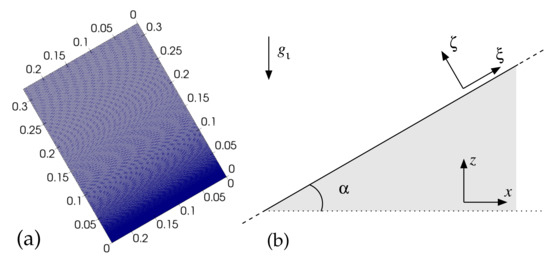
Figure 1.
Sketch of the validation case setting: (a) front view of the computational domain and grid; (b) outline of the geometry of the inclined and heated infinite plane. Note that the domain is 3D and includes the (spanwise) y-direction, which is of spatial homogeneity.
3.1. Validation Case Setup
The validation is made against the DNS by Giometto et al. [43], which imposes a constant temperature at the slope and a background thermal stratification. Particularly, the case U30H is reproduced and the results are expressed in terms of buoyancy field b rather than temperature variation. The flow regime corresponds to with a slope inclination of and the air viscosity . Quantities are made non-dimensional by means of system characteristic length , velocity , and buoyancy . The non-dimensional time is , which defines a characteristic time period.
The computational domain is shown in Figure 1a and is three-dimensional, including the (spanwise) y-direction. Its extension in the non-dimensional unit is in the -, y-, -direction, respectively. The mesh counts cells, which are stretched near the slope surface by a hyperbolic tangent function [60] to ensure that the wall-boundary layer is directly resolved. To this end, the first cell near the slope has the same height as the cell in the reference DNS.
To simulate an infinite slope, cyclic conditions are imposed at the boundaries perpendicular to the slope. The top boundary simulates a free interface (zero-gradient condition for all the variables). At the slope, a non-slip condition for velocity m/s, constant positive surface buoyancy m/s and zero-gradient for other variables is imposed. A sponge region of zero gravity force m/s is imposed in a region corresponding to the of the top of the domain to avoid possible numerical instability, as suggested in Giometto et al. [43].
The simulation is run for time periods and the statistics are collected in the last , when the statistical steady-state configuration is reached. Quantities are averaged along the streamwise () and spanwise (y) directions, as well as in time. The root-mean-square (RMS) are computed as , where is a generic variable and the angular brackets denote the space-time average.
3.2. Validation Results
First- and second-order statistics from LES are reported and compared with the reference DNS [43]. The analyses are performed in the system of reference of the slope; thus, the profiles are taken along the slope-normal direction.
Figure 2a shows the non-dimensional averaged profiles of streamwise velocity and buoyancy, as well as the RMS of velocity components and buoyancy magnitude. The LES mean profiles practically collapse onto the DNS profiles. The velocity RMS components are slightly underestimated by the LES in a region very close to the slope, where the convective motion is more energetic. The buoyancy RMS reproduces the peak at even if its intensity is slightly overestimated.
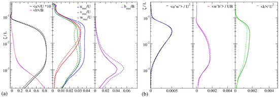
Figure 2.
Non-dimensional average quantities along a slope-normal line. Solid lines, DNS by [43]; dashed lines, present LES. Left panel (a): streamwise velocity u and buoyancy b, root-mean-square of velocity components, and root-mean-square of buoyancy force. Right panel (b): turbulent kinematic momentum flux , turbulent buoyancy flux and turbulence kinetic energy k.
Figure 2b displays the slope-normal profiles of non-dimensional turbulent kinematic momentum and buoyancy fluxes, and the resolved turbulence kinetic energy . Turbulent fluxes are in very good agreement with the reference profiles, while the LES turbulence kinetic energy exhibits a limited underestimation consistent with RMS profiles.
Overall, the accuracy of the mean and turbulent fields is satisfactory, despite minor discrepancies in the RMS profiles. Thus, the present simulation approach allows to effectively reproduce the thermo-fluid dynamic of the system. The LES results are then applied for simulating anabatic flows in the case study described and analysed in the following sections.
4. Case Study Setup
The anabatic flow along a finite slope uniformly heated is studied in a typical geometry of a laboratory experiment [28,32,61]. Figure 3b sketches the case setup: a double slope is placed in the centre of a water tank with dimensions of m, respectively, for width (x), depth (y) and height (z). The slope is m long, inclined of an angle with respect to the ground, and heated up of K compared to water. Such difference of temperature has been chosen to generate an average heat flux at the slope equal to W/m, where is the heat flux density at the slope, the temperature normal gradient, is the water specific heat at constant pressure, and is the area of the slope. The physical parameters for water are: thermal expansion K, laminar and turbulent Prandtl numbers and , respectively. The boundaries of the tank are solid walls, except for the front () and back () vertical boundaries to which a cyclic boundary condition is imposed to make the domain virtually infinite along the direction of homogeneity (y).
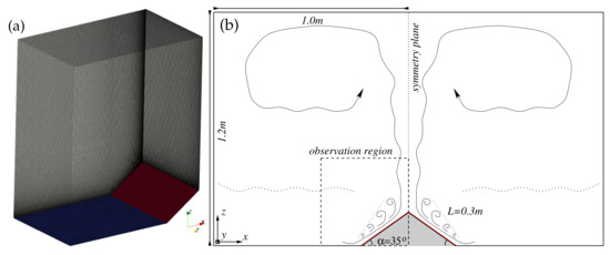
Figure 3.
Outline of the case study geometry: (a) overview of the simulation domain and computational grid; (b) sketch of the full geometry and the main flow features, highlighting the observation region selected for the analyses.
It is worth highlighting that the configuration chosen for the present work is representative of experimental studies in a water tank, which are characterised by low compared to the real-system configuration. Schumann [38] showed that atmospheric flow can be reproduced by using wall functions, i.e., modelling the near-ground physics to reduce the computational cost of the simulation. This allows the simulation of high- flows but does not directly resolve the slope-boundary layer and the underlying physical mechanisms, which are the focus of the present work. For this reason, the study is concerned with highly resolved flow at low .
The domain height and width are large enough to ensure that thermal convection along the slope reaches a configuration of equilibrium for a period of time sufficiently long to collect statistics. During this period, the influence of the boundaries is limited to the upper part of the tank. The analyses are focused on an observation region surrounding the slope, not significantly affected by the overall tank circulation (see discussion of Figure 4). The extension of the observation region is in the x- and z-directions and the entire domain in the y-direction.
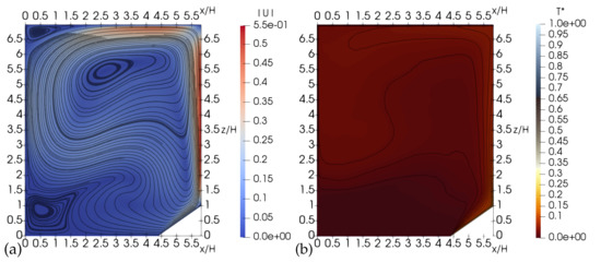
Figure 4.
Distribution of velocity and temperature perturbation in the entire computational domain: (a) non-dimensional average velocity magnitude and streamlines across the entire computational domain; (b) non-dimensional average temperature perturbation distribution and contour lines at 100 equally spaced values are reported as black solid lines. Particularly, contour lines at levels (from bottom to top) are clearly visible.
The characteristic length is chosen to be the height of the slope and the characteristic velocity is the buoyant velocity . In such a way, the characteristic velocity is higher when the slope is more inclined and reduces to zero when it is horizontal (i.e., when no anabatic flow develops). Consequently, the characteristic time scale is and the Rayleigh number of the system is , indicating a fully turbulent regime.
4.1. Computational Grid, Initial and Boundary Conditions
Taking advantage of the symmetry of the problem along the vertical plane at the mid-width (see Figure 3b), the computation domain is reduced to half of the tank and a symmetry boundary condition is applied to virtually simulate the remaining part. This reduces the computational cost without losing information about the physics of the problem.
Figure 3a displays the numerical mesh, which is structured and staggered, composed of cells in the x-,y-,z-direction respectively. A hyperbolic tangent stretching [60] is applied to vertical (z) and horizontal (x) directions in order to increase the resolution near the slope and the symmetry plane, where the more energetic motion is localised. In the vertical direction, the smallest cell at the slope surface is m high. Preliminary simulations have been run to state that the slope-boundary layer is directly resolved, i.e., ensuring that the first computational point at the slope is within (where is the friction velocity) [62]. Such preliminary simulations have been performed on several meshes with an increased resolution above the slope and increasing stretching at the slope surface. Particularly, three meshes have been tested with an overall increase of about of cells in all directions above the slope (in the observation region). The present mesh is the intermediate between the three since the additional increment of points does not change the first- and second-order statistics.
In order to discuss the grid quality, as well as to assess the range of turbulence scales captured by the computational grid, the power spectra are reported [63,64]. Figure 5 shows the power spectra of velocity components and temperature perturbation in the system of reference of the slope. Data are collected in time at three selected points, which are placed at the mid-slope and at increasing distance from the surface (within the region where the most energetic anabatic flow develops, see also Figure 6). Velocity power spectra exhibit the slope characteristic for the inertial range, while the steeper slope is associated with the inertial-diffusive range for buoyancy-driven flows [63]. In the temperature perturbation spectra, a decay of slope is detectable. These verified that the inertial range is covered by the computational mesh adopted, which is a requirement for performing an LES. In addition, the value of is compared with the molecular kinematic viscosity , by scrutinising the ratio . Such parameter measures the contribution of the sub-grid scale with respect to the computational mesh used: indicates that the LES reduces to a quasi DNS, means a high contribution of turbulent model and thus a coarse spatial resolution, while corresponds to and suggests a good mesh resolution [55,64]. In the region above the slope where the largest part of the anabatic flow is localised, indicating that the correction due to the turbulent model is limited and that the turbulent kinetic energy is dissipated mainly by the resolved scale of motion than the sub-grid scales. Hence, the spatial resolution can be considered satisfactory.
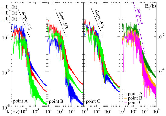
Figure 5.
Power spectra of the three velocity components in the system of reference of the slope () and temperature perturbation () at three selected points within the convective region near the slope. Points placed at different heights at the slope-normal line passing through the slope mid-point (): point A (), point B (), point C ().
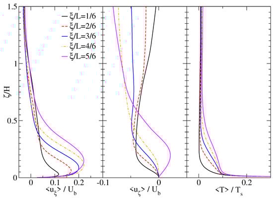
Figure 6.
Non-dimensional mean slope-parallel velocity , slope-normal velocity and temperature perturbation at selected lines perpendicular to the slope: five levels equally spaced from the slope base to its apex .
The boundary conditions are: at the ground and at the slope, the velocity enforces the non-slip condition, pressure and turbulent quantities have zero-gradient. The temperature is set to constant value at the slope and to reference temperature elsewhere. At the top and lateral walls, the Spalding wall function [65] is applied to velocity and pressure, while turbulent quantities enforce the zero-gradient condition and temperature is constant . Wall functions are applied since the analyses are not focused on the far-slope dynamics and high accuracy is not required. As mentioned above, the symmetry condition is applied to all variables at the symmetry plane [57]. The front and back boundaries are cyclic. As the initial condition, the water is neutrally stratified (), at the constant temperature K, and at rest ().
4.2. Overall Circulation
The simulation is run for more than . The velocity time-series at selected locations in the proximity of the slope (not reported) indicate that the flow reaches a stable configuration after from the initialisation. The statistics are collected for a period of after reaching the stable configuration. Quantities are averaged in time and space, along the spanwise direction.
The overall circulation within the tank is briefly described. Figure 4a shows the non-dimensional mean velocity magnitude and streamlines across the entire computational domain. The circulation is driven by natural convection generated at the heated slope. The flow increases its intensity from the slope base to the apex, where it separates from the surface and gives rise to an ascending flow. A principal vortex dominates the top-tank zone (), while the bottom-tank zone () is not impacted by the principal vortex. At the vortex centre, the fluid is almost at rest. The hot fluid is carried downward from the top-tank zone by the principal vortex and comes in contact with the cold fluid in the bottom-tank zone (on the opposite side to the slope location). The average temperature of the top-tank is increased by the injection of hot fluid, transported by the ascending flow and mixed by the principal vortex. Instead, the bottom part practically maintains the initial temperature (see Figure 4b). The result is that the more energetic part of the descending flow from the top-tank deviates horizontally in the range . Above the slope, the principal vortex bends towards the slope. However, the weak velocity intensity of this downward flow does not substantially influence the highly energetic anabatic flow near the slope (see also the discussion of Figure 6 and Figure 7). In the following Section 5, the focus is restricted to the observation region to detail the thermal and dynamic characteristics of the anabatic flow.
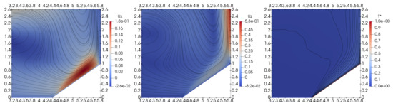
Figure 7.
Spatial distribution of non-dimensional mean velocity components in horizontal and vertical directions (streamlines are superimposed), together with temperature (contour lines at 100 equally spaced values are reported as black solid lines). Vertical plane normal to spanwise direction, reduced to the observation region.
5. Results and Discussion
The anabatic flow along the slope is investigated by analysing the first- and second-order statistics distribution at a vertical plane normal to the spanwise direction (y) and along selected lines perpendicular to the slope surface. Three-dimensional and instantaneous turbulent features are also visualised and described.
5.1. First-Order Statistics
Figure 7 shows the spatial distribution of non-dimensional mean velocity components and temperature in the observation region. The higher values of horizontal velocity are mainly localised in a limited layer above the slope, where the anabatic flow develops. Hereafter, we refer to this region as the convective layer. The thickness of such a layer is almost zero at the slope base and increases approaching the apex, before being deteriorated by the ascending flow. It does not exceed in the slope-normal direction, where the velocity and temperature perturbation profiles at (that are less affected by the flow conditions at the of the slope edges) practically collapse on the same profile. An accurate definition of the layer thickness development is not reported since it requires a dedicated analysis that is beyond the aims of the present study. The streamlines show that the anabatic flow produces a weak horizontal flow that drives the fluid close to the ground towards the slope. The vertical velocity reaches the highest values above the slope apex (), which is dominated by the ascending flow. Low positive values are also detectable in the convective layer. The streamlines highlight the presence of a weak downward flow from the top-tank zone (as discussed in Section 4.2). Above the centre of the slope, the flow is almost slope-normal directed, while being deviated in slope-parallel direction by the anabatic flow. The temperature distribution shows that the larger temperature perturbation is located extremely close to the slope surface. The contour lines follow the mean velocity field, except for the line at that deviates horizontally and stabilises at height in the bottom-tank zone. This confirms that the fluid is not stratified at the bottom part of the tank, while an unstable stratification increases climbing the slope.
Figure 6 shows the profiles of the non-dimensional mean velocity components (slope-parallel and slope-normal ) and temperature, taken at five slope-normal lines equally distributed from the base to the apex of the slope. The profiles of the slope-parallel velocity are characterised by a rapid increase of velocity near the slope until a peak is reached, and subsequent decay to an edge-point above which the velocity shows a quasi-linear behaviour. As the apex of the slope is approached, the velocity exhibits a larger peak, which is displaced further away from the slope. Consistently, the region characterised by positive velocity and the edge-point increases in height. The profile at level shows the influence of the ascending flow, which prevents the growth of the velocity peak and transport momentum towards the slope-normal direction. The slope-normal velocity profiles show negative values in the convective layer (), except at level where the ascending flow dominates. These velocities are one order of magnitude smaller than the slope-parallel ones. Negative velocities are due to the presence of the ground, and they are not present in the infinite slope case (see Figure 2a): the flow that reaches the slope from the left side of the bottom-tank is directed parallel to the ground; thus, the velocity that impacts the slope has a negative component in the slope-normal direction. The local minimum of velocity has an almost constant value , and its elevation approximately coincides with the height of the edge-point of slope-parallel velocity. In the surrounding area (), the vertical velocity is expected to tend to zero, but negative values are detectable. They are mainly generated by the downward flow from the tanks upper part. Temperature perturbation displays an exponential-decay layer (), where all the profiles decay exponentially below and practically collapse to the same curve (estimation done on non-reported profiles in logarithmic scale). This is a conductive layer where conduction dominates over convection. Above, there is the convective layer, where temperature experiences an almost linear decrease. The temperature maintains higher values as the apex is approached. Far from the slope surface (), the temperature field is almost unperturbed.
5.2. Second-Order Statistics
Figure 8 presents the distribution of turbulent kinematic momentum and heat fluxes at a vertical plane in the observation region. The momentum flux exhibits large positive values close to the slope surface and also in the final part of the convective layer (corresponding to ), with a peak in the vertical range . This is the area where the downward flow from the upper part of the tank came in contact with the upper boundary of the convective layer and is deviated horizontally (see Figure 7), producing a positive spot of turbulent flux. The vertical heat flux assumes positive values in the convective layer, with a climax at the slope surface and above the apex where the ascending flow rises. They denote the tendency of turbulence to diffuse temperature upward within the convective layer.
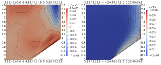
Figure 8.
Turbulent kinematic momentum flux and vertical heat flux made non-dimensional and averaged. Distribution at a vertical plane, normal to the spanwise direction and reduced to the observation region.
Figure 9 displays the profiles of turbulent kinematic momentum and heat fluxes, as well as the turbulence kinetic energy and temperature perturbation RMS along selected slope-normal lines, in the system of reference of the slope. The turbulent momentum flux has a maximum that corresponds to the inflexion point of the mean velocity component profiles in Figure 6, as predicted by the gradient-diffusion hypothesis. Above the maximum, all profiles rapidly decrease and reach an almost constant value approximately at the same height of the edge-point of the slope-parallel velocity. Hence, positive fluxes are confined in the convective layer. As expected, the intensity increases as the apex is approached and the main flow became more energetic. Turbulent slope-parallel heat fluxes show a strong peak within the conductive layer, where all the profiles practically overlap. In the convective layer, fluctuations have an almost linear decrease and assume zero values in the outer region. Turbulent slope-normal heat fluxes peak around , where the mean temperature profiles have inflexion points. They also tend to zero in the outer region. Both sets of vertical and horizontal profiles indicate that turbulent diffusion is limited in the convective layer and acts to diffuse temperature in slope-parallel and -normal directions. The positive values of turbulence kinetic energy are confined near the slope. Moving from the base to the apex of the slope, the intensity of k and the elevation of the profile peak increase. This is in accordance with the turbulent momentum flux and the slope-parallel velocity component. The profiles of temperature RMS exhibit a maximum at , i.e., the limit of the conductive layer. This is expected because of the strong thermal gradient arising at the interface. Above, these profiles rapidly decrease to zero and collapse almost onto the same curve within the convective layer, except for the line that has an even more rapid decay.
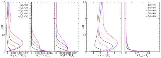
Figure 9.
Non-dimensional mean turbulent quantities in the system of reference of the slope: turbulent kinematic momentum flux , slope-parallel turbulent heat flux , slope-normal turbulent heat flux , turbulence kinetic energy , temperature perturbation RMS . Profiles along selected slope-normal lines (same as in Figure 7).
Overall, three main regions of motion are detectable and qualitatively described in terms of dynamic and thermal characteristics:
- Conductive layer:
- The thin region close to the slope surface () where the slope-parallel velocity rapidly increases, temperatures following an exponential decay, and slope-parallel heat fluxes turbulent flows reach their maximum. Slope-normal heat transfer is dominated by conduction.
- Convective layer:
- The layer above the slope where the anabatic flow mainly develops, corresponding to the region of largest slope-parallel velocity component and most energetic turbulent fluxes. Temperature profiles display an almost linear decrease, and the layer thickness increases along the slope before being destroyed by the ascending flow.
- Outer region:
- Relatively far from the slope (). The velocity loses most of the energy generated by the buoyancy force at the slope, the temperature perturbation is almost negligible, and turbulent fluxes decay to low values. This region is almost unperturbed by the slope anabatic flow.
As already mentioned, the convective layer is still in evolution and does not reach a stable thickness in this configuration. For better analysis and quantification of such a layer, a more extended slope or a case study at higher would be required.
5.3. Turbulent Structures
Taking advantage of the opportunity given by the LES to reproduce instantaneous turbulent fields, the turbulent structures arising in the anabatic flow are analysed here.
Figure 10a shows the non-dimensional instantaneous temperature perturbation at the plane , i.e., vertical and perpendicular to the slope. The temperature distribution reveals the presence of turbulent thermal plumes within the convective layer. Such plumes are generated near the slope base by thermal instabilities arising in the proximity of the surface. Subsequently, they grow vertically as they are transported along the slope by the anabatic flow. Near the slope apex, the plumes start to deteriorate and are finally destroyed by the ascending flow.
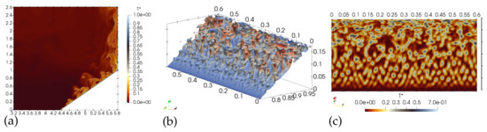
Figure 10.
Non-dimensional instantaneous temperature perturbation at the last time-step simulated: (a) vertical plane in the observation region, contour lines at ; (b) three-dimensional isothermal surface above the slope; (c) plane parallel to the slope and close to the surface (distance ).
Figure 10b displays the three-dimensional structures of the turbulent thermal plumes through the visualisation of the isothermal surface . Plumes emerge near the slope base as a sort of high-temperature bubble, which rapidly increases their height. At the centre of the slope, they are elongated in the vertical direction and presents a cylindrical base that is curved in the slope-parallel direction at the top. This hook-like shape is due to the main flow, which transports the plumes parallel to the slope. Near the apex of the slope, it is worth noticing that the axis of the plumes rotates to be almost horizontal before being destroyed by the ascending flow.
Figure 10c reports the temperature distribution near the slope surface (distance ) to better understand the mechanism that triggers the rise of a thermal plume. Spots of high temperature are clearly detectable in the proximity of the slope surface, at the boundary between the conductive layer and the convective layer. They can be interpreted as a periodic perturbation of the conductive layer, and a careful visualisation of the plumes reveals that there is a thermal spot at the base of each of them. Such thermal spots are possibly generated when the cold flow from the bottom-tank impacts the hot slope surface. The strong unstable thermal gradient produces thermal instabilities (similar to the Taylor instabilities) in the conductive layer. Such instabilities give rise to the thermal plumes and are transported along the slope. Near the apex, the plumes detached from the thermal spots: the former are rotated horizontally by the main flow before being destroyed by the ascending flow; the latter merge together and produce structure elongated in the spanwise direction in the proximity of the slope apex.
Figure 11 summarises the structure and the evolution of turbulent thermal plumes. Their evolution along the slope can be divided into three main regions:
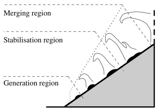
Figure 11.
Conceptualisation of the turbulent thermal structures arising in the anabatic flow and their evolution along the slope.
- Generation region (): Spots are almost absent at the bottom edge of the slope. The weak thermal instabilities are generated, but plumes are almost not detectable.
- Stabilisation region (): Spots assume an almost circular shape and the central temperature increases. Plumes emerge and develop in the convective layer, assuming their hook-line shape.
- Merging region (): Spots merge together while they are transported near the apex, where they appear elongated spanwise and are destroyed. Plumes detached from the surface and their axis is rotated horizontally. They are transported by the main flow and eventually destroyed by the highly energetic ascending flow.
Thermal plumes are turbulent structures confined within the convective layer and mainly develops vertically, thus transporting temperature from the slope surface across the convective layer. They can be responsible for the high level of turbulent thermal fluxes (see Figure 8) and contribute to the temperature mixing, which results in the almost linear profile of the temperature in the convective layer. Therefore, such structures play a crucial role in the dynamics of the convective layer and in the processes of vertical transport and mixing.
6. Conclusions
The high-resolved large-eddy simulation (LES) methodology is used to study an anabatic flow in a simplified geometry consisting in a uniformly heated double slope in an isothermal water tank. The configuration chosen reproduces the common setup of laboratory experiments. The Rayleigh number of the flow is (fully turbulent regime) and the simulation is three-dimensional and time-dependent, enabling the analysis of instantaneous turbulent characteristics. To the best of the authors’ knowledge, this is the first LES specifically designed to evaluate the turbulent dynamics of an anabatic flow in a simplified setup.
The numerical approach is successfully validated against direct numerical simulations of an idealised case. Subsequently, the first- and second-order statistics of the selected case study are discussed. The overall tank dynamics shows that the anabatic flow generates a principal recirculation vortex, which is confined in the top part of the tank and does not significantly influence the development of the anabatic flow. The dynamics in the proximity of the slope are characterised by the presence of three characteristic regions: (i) the conductive layer, very close to the hot surface where temperature decreases exponentially and velocity rapidly increases; (ii) the convective layer dominated by convection, where the temperature has an almost linear decrease with the distance from the slope, and the most energetic mean and turbulent motions are confined; (iii) the outer region, which is almost unperturbed.
The analysis of instantaneous fields reveals the presence of thermal plumes, sketched in Figure 11. They are periodic turbulent structures continuously generated in the proximity of the slope base, transported along the slope and destroyed near the apex. These plumes arise from the vertical motions triggered by the thermal instabilities at the boundary between the conductive layer and the convective layer. Thermal plumes are confined into the convective layer and enhance vertical transport of momentum and heat, increasing the turbulence intensity and the mixing within the layer.
The present contribution gives the first description of such structures, which are described with respect to the anabatic flow dynamics. Additional analyses will be reported in future works.
Author Contributions
Data curation, D.D.S.; Investigation, Methodology, and Writing—original draft, C.C.; Supervision, S.D.S.; Writing—review and editing, F.B. All authors have read and agreed to the published version of the manuscript.
Funding
This work has received funding from the OPERANDUM project funded by the European Union’s H2020 Research and Innovation programme (H2020-SC5-08-2017) funded under the Grant Agreement No. 776848.
Institutional Review Board Statement
Not applicable.
Informed Consent Statement
Not applicable.
Data Availability Statement
Not applicable.
Acknowledgments
The authors acknowledge the use of computational resources from the parallel computing cluster of the Open Physics Hub at the Physics and Astronomy Department in Bologna.
Conflicts of Interest
The authors declare no conflict of interest.
References
- Whiteman, D.C. Observations of Thermally Developed Wind Systems in Mountainous Terrain. In Atmospheric Processes over Complex Terrain; Blumen, W., Ed.; American Meteorological Society: Boston, MA, USA, 1990; pp. 5–42._2. [Google Scholar] [CrossRef]
- Monti, P.; Fernando, H.; Princevac, M.; Chan, W.; Kowalewski, T.; Pardyjak, E. Observations of Flow and Turbulence in the Nocturnal Boundary Layer over a Slope. J. Atmos. Sci. 2002, 59. [Google Scholar] [CrossRef]
- Rampanelli, G.; Zardi, D.; Rotunno, R. Mechanisms of Up-Valley Winds. J. Atmos. Sci. 2004, 61, 3097–3111. [Google Scholar] [CrossRef]
- Rotach, M.; Zardi, D. On the Boundary Layer Structure over Highly Complex Terrain: Key Findings from MAP and Related Projects; Hrvatski Meteoroloski Casopis: Zagreb, Croatia, 2005; pp. 124–127. [Google Scholar]
- Fernando, H.J.S. Fluid dynamics of urban atmospheres in complex terrain. Annu. Rev. Fluid Mech. 2008, 42, 365–389. [Google Scholar] [CrossRef]
- Zardi, D.; Whiteman, C. Diurnal Mountain Wind Systems. Mt. Weather. Res. Forecast. 2013, 35–119._2. [Google Scholar] [CrossRef]
- Jensen, D.; Nadeau, D.; Hoch, S.; Pardyjak, E. Observations of Near-Surface Heat-Flux and Temperature Profiles Through the Early Evening Transition over Contrasting Surfaces. Bound. Layer Meteorol. 2015, 159. [Google Scholar] [CrossRef]
- Princevac, M.; Fernando, H. A criterion for the generation of turbulent anabatic flows. Phys. Fluids 2007, 19, 105102. [Google Scholar] [CrossRef]
- Hunt, J.; Fernando, H.; Princevac, M. Unsteady thermally driven flows on gentle slopes. J. Atmos. Sci. 2003, 60, 2169–2182. [Google Scholar] [CrossRef]
- Serafin, S.; Adler, B.; Cuxart, J.; De Wekker, S.F.J.; Gohm, A.; Grisogono, B.; Kalthoff, N.; Kirshbaum, D.J.; Rotach, M.W.; Schmidli, J.; et al. Exchange Processes in the Atmospheric Boundary Layer Over Mountainous Terrain. Atmosphere 2018, 9, 102. [Google Scholar] [CrossRef]
- Princevac, M.; Fernando, H. Morning breakup of cold pools in complex terrain. J. Fluid Mech. 2008, 616, 99. [Google Scholar] [CrossRef]
- Nadeau, D.F.; Oldroyd, H.J.; Pardyjak, E.R.; Sommer, N.; Hoch, S.W.; Parlange, M.B. Field observations of the morning transition over a steep slope in a narrow alpine valley. Environ. Fluid Mech. 2018, 20, 1–22. [Google Scholar] [CrossRef]
- Grubišić, V.; Doyle, J.; Kuettner, J.; Mobbs, S.; Smith, R.; Whiteman, C.; Dirks, R.; Czyzyk, S.; Cohn, S.; Vosper, S.; et al. The Terrain-Induced Rotor Experiment: An overview of the field campaign and some highlights of special observations. Bull. Amer. Meteor. Soc. 2008, 89, 1513–1533. [Google Scholar] [CrossRef]
- Serafin, S.; Zardi, D. Structure of the Atmospheric Boundary Layer in the Vicinity of a Developing Upslope Flow System: A Numerical Model Study. J. Atmos. Sci. 2010, 67, 1171–1185. [Google Scholar] [CrossRef]
- De Wekker, S.F.J. Observational and Numerical Evidence of Depressed Convective Boundary Layer Heights near a Mountain Base. J. Appl. Meteorol. Climatol. 2008, 47, 1017–1026. [Google Scholar] [CrossRef]
- Serafin, S.; Zardi, D. Daytime Heat Transfer Processes Related to Slope Flows and Turbulent Convection in an Idealized Mountain Valley. J. Atmos. Sci. 2010, 67, 3739–3756. [Google Scholar] [CrossRef]
- De Wekker, S.F.; Kossmann, M. Convective boundary layer heights over mountainous terrain—A review of concepts. Front. Earth Sci. 2015, 3, 77. [Google Scholar] [CrossRef]
- Finnigan, J.; Ayotte, K.; Harman, I.; Katul, G.; Oldroyd, H.; Patton, E.; Poggi, D.; Ross, A.; Taylor, P. Boundary-Layer Flow over complex topography. Bound.-Layer Meteorol. 2020, 177, 247–313. [Google Scholar] [CrossRef]
- Prandtl, L. Fuhrer Durch Die Stromungslehre; Veweg und Sohn: Wiesbaden, Germany, 1942; pp. 373–375. [Google Scholar]
- Defant, F. Local Winds. In Compendium of Meteorology; Malone, T.F., Ed.; American Meteorological Society: Boston, MA, USA, 1951. [Google Scholar] [CrossRef]
- Egger, J. Linear two-dimensional theory of thermally induced slope winds. Contrib. Atmos. Phys. 1981, 54, 465–481. [Google Scholar]
- Ye, Z.J.; Segal, M.; Pielke, R.A. Effects of Atmospheric Thermal Stability and Slope Steepness on the Development of Daytime Thermally Induced Upslope Flow. J. Atmos. Sci. 1987, 44, 3341–3354. [Google Scholar] [CrossRef]
- Kavčič, I.; Grisogono, B. Katabatic flow with Coriolis effect and gradually varying eddy diffusivity. In Atmospheric Boundary Layers: Nature, Theory and Applications to Environmental Modelling and Security; Baklanov, A., Grisogono, B., Eds.; Springer: New York, NY, USA, 2007; pp. 221–231. [Google Scholar] [CrossRef]
- Zardi, D.; Serafin, S. An analytic solution for time-periodic thermally driven slope flows. Q. J. R. Meteorol. Soc. 2015, 141, 1968–1974. [Google Scholar] [CrossRef]
- Guttler, I.; Marinovic, I.; Večenaj, Ž.; Grisogono, B. Energetics of Slope Flows: Linear and Weakly Nonlinear Solutions of the Extended Prandtl Model. Front. Earth Sci. 2016, 4. [Google Scholar] [CrossRef]
- Whiteman, C.D. Breakup of temperature inversions in deep mountain valleys: Part I. Observations. J. Appl. Meteorol. Climatol. 1982, 21, 270–289. [Google Scholar] [CrossRef]
- Kader, B.; Yaglom, A. Mean fields and fluctuation moments in unstably stratified turbulent boundary layers. J. Fluid Mech. 1990, 212, 637–662. [Google Scholar] [CrossRef]
- Moroni, M.; Cenedese, A. Laboratory Simulations of Local Winds in the Atmospheric Boundary Layer via Image Analysis. Adv. Meteorol. 2015, 2015, 1–34. [Google Scholar] [CrossRef]
- Perry, S.; Snyder, W. Laboratory simulations of the atmospheric mixed-layer in flow over complex topography. Phys. Fluids 2017, 29, 020702. [Google Scholar] [CrossRef]
- Reuten, C.; Steyn, D.G.; Allen, S.E. Water tank studies of atmospheric boundary layer structure and air pollution transport in upslope flow systems. J. Geophys. Res. (Atmos.) 2007, 112. [Google Scholar] [CrossRef]
- Crook, N.A.; Tucker, D.F. Flow over Heated Terrain. Part I: Linear Theory and Idealized Numerical Simulations. Mon. Weather Rev. 2005, 133, 2552–2564. [Google Scholar] [CrossRef]
- Hocut, C.; Liberzon, D.; Fernando, H. Separation of upslope flow over a uniform slope. J. Fluid Mech. 2015, 775, 266–287. [Google Scholar] [CrossRef]
- Goldshmid, R.H.; Bardoel, S.L.; Hocut, C.M.; Zhong, Q.; Liberzon, D.; Fernando, H.J. Separation of upslope flow over a plateau. Atmosphere 2018, 9, 165. [Google Scholar] [CrossRef]
- Skyllingstad, E.D. Large-eddy simulation of katabatic flows. Bound. Layer Meteorol. 2003, 106, 217–243. [Google Scholar] [CrossRef]
- Grisogono, B.; Axelsen, S. A Note on the Pure Katabatic Wind Maximum over Gentle Slopes. Bound. Layer Meteorol. 2012, 142, 527–538. [Google Scholar] [CrossRef]
- Axelsen, S.L.; van Dop, H. Large-eddy simulation of katabatic winds. Part 1: Comparison with observations. Acta Geophys. 2009, 57, 803–836. [Google Scholar] [CrossRef]
- Axelsen, S.L.; van Dop, H. Large-eddy simulation of katabatic winds. Part 2: Sensitivity study and comparison with analytical models. Acta Geophys. 2009, 57, 837–856. [Google Scholar] [CrossRef]
- Schumann, U. Large-eddy simulation of the up-slope boundary layer. Q. J. R. Meteorol. Soc. 1990, 116, 637–670. [Google Scholar] [CrossRef]
- Dörnbrack, A.; Schumann, U. Numerical simulation of turbulent convective flow over wavy terrain. Bound.-Layer Meteorol. 1993, 65, 323–355. [Google Scholar] [CrossRef]
- Anquetin, S.; Guilbaud, C.; Chollet, J.P. The formation and destruction of inversion layers within a deep valley. J. Appl. Meteorol. 1998, 37, 1547–1560. [Google Scholar] [CrossRef]
- Luo, Z.; Li, Y. Passive urban ventilation by combined buoyancy-driven slope flow and wall flow: Parametric CFD studies on idealized city models. Atmos. Environ. 2011, 45, 5946–5956. [Google Scholar] [CrossRef]
- Fedorovich, E.; Shapiro, A. Structure of numerically simulated katabatic and anabatic flows along steep slopes. Acta Geophys. 2009, 57, 981–1010. [Google Scholar] [CrossRef]
- Giometto, M.G.; Katul, G.G.; Fang, J.; Parlange, M.B. Direct numerical simulation of turbulent slope flows up to Grashof number Gr = 2.1×10¹¹. J. Fluid Mech. 2017, 829, 589–620. [Google Scholar] [CrossRef]
- Talbot, C.; Bou-Zeid, E.; Smith, J. Nested Mesoscale Large-Eddy Simulations with WRF: Performance in Real Test Cases. J. Hydrometeorol. 2012, 13, 1421–1441. [Google Scholar] [CrossRef]
- Catalano, F.; Cenedese, A. High-resolution numerical modeling of thermally driven slope winds in a valley with strong capping. J. Appl. Meteorol. Climatol. 2010, 49, 1859–1880. [Google Scholar] [CrossRef]
- Chow, F.K.; Weigel, A.P.; Street, R.L.; Rotach, M.W.; Xue, M. High-resolution large-eddy simulations of flow in a steep Alpine valley. Part I: Methodology, verification, and sensitivity experiments. J. Appl. Meteorol. Climatol. 2006, 45, 63–86. [Google Scholar] [CrossRef]
- Golaz, J.C.; Doyle, J.D.; Wang, S. One-way nested large-eddy simulation over the Askervein Hill. J. Adv. Model. Earth Syst. 2009, 1. [Google Scholar] [CrossRef]
- Weigel, A.P.; Chow, F.K.; Rotach, M.W.; Street, R.L.; Xue, M. High-resolution large-eddy simulations of flow in a steep Alpine valley. Part II: Flow structure and heat budgets. J. Appl. Meteorol. Climatol. 2006, 45, 87–107. [Google Scholar] [CrossRef]
- Châtelain, A.; Ducros, F.; Métais, O. LES of turbulent heat transfer: Proper convection numerical schemes for temperature transport. Int. J. Numer. Methods Fluids 2004, 44, 1017–1044. [Google Scholar] [CrossRef]
- Fedorovic, E.; Shapiro, A. Turbulent natural convection along a vertical plate immersed in a stably stratified fluid. J. Fluid Mech. 2009, 636, 41–57. [Google Scholar] [CrossRef]
- Sagaut, P. Large Eddy Simulation for Incompressible Flows. An Introduction; Springer: Berlin/Heidelberg, Germany, 2000. [Google Scholar]
- Pope, S. Turbulent Flows; Cambridge University Press: Cambridge, UK, 2000. [Google Scholar]
- Smagorinsky, J. general circulation experiments with the primitive equations: I. The basic experiment. Mon. Weather Rev. 1963, 91, 99. [Google Scholar] [CrossRef]
- Van Driest, E. On turbulent flow near a wall. J. Aeronaut. Sci. 1956, 23, 1007–1011. [Google Scholar] [CrossRef]
- Cintolesi, C.; Petronio, A.; Armenio, V. Turbulent structures of buoyant jet in cross-flow studied through large-eddy simulation. Environ. Fluid Mech. 2019, 19, 401–433. [Google Scholar] [CrossRef]
- Cintolesi, C.; Pulvirenti, B.; Di Sabatino, S. Large-Eddy Simulations of Pollutant Removal Enhancement from Urban Canyons. Bound. Layer Meteorol. 2021. [Google Scholar] [CrossRef]
- OpenFOAM. The OpenFOAM Foundation. Version 6.0. Available online: https://openfoam.org/ (accessed on 1 May 2019).
- Jasak, H.; Weller, H.; Gosman, A. High resolution NVD differencing scheme for arbitrarily unstructured meshes. Int. J. Numer. Meth. Fluids 1999, 31, 431–449. [Google Scholar] [CrossRef]
- Trivellato, F.; Raciti Castelli, M. On the Courant–Friedrichs–Lewy criterion of rotating grids in 2D vertical-axis wind turbine analysis. Renew. Energy 2014, 62, 53–62. [Google Scholar] [CrossRef]
- Cintolesi, C.; Petronio, A.; Armenio, V. Large eddy simulation of turbulent buoyant flow in a confined cavity with conjugate heat transfer. Phys. Fluids 2015, 27. [Google Scholar] [CrossRef]
- Smith, C.M.; Skyllingstad, E.D. Numerical Simulation of Katabatic Flow with Changing Slope Angle. Mon. Weather Rev. 2005, 133, 3065–3080. [Google Scholar] [CrossRef]
- Piomelli, U.; Balaras, E. Wall-Layer Models for Large-Eddy Simulations. Annu. Rev. Fluid Mech. 2002, 34, 349–374. [Google Scholar] [CrossRef]
- De Wit, L.; van Rhee, C.; Keetels, G. Turbulent Interaction of a Buoyant Jet with Cross-Flow. J. Hydraul. Eng. 2014, 140, 04014060. [Google Scholar] [CrossRef]
- Cavar, D.; Meyer, K.E. LES of turbulent jet in cross-flow: Part 1 – A numerical validation study. Int. J. Heat Fluid Flow 2012, 36, 18–34. [Google Scholar] [CrossRef]
- Launder, B.; Spalding, D. The numerical computation of turbulent flows. Comput. Methods Appl. Mech. Eng. 1974, 2, 263–289. [Google Scholar] [CrossRef]


Publisher’s Note: MDPI stays neutral with regard to jurisdictional claims in published maps and institutional affiliations. |
© 2021 by the authors. Licensee MDPI, Basel, Switzerland. This article is an open access article distributed under the terms and conditions of the Creative Commons Attribution (CC BY) license (https://creativecommons.org/licenses/by/4.0/).