Article

Analysis of Ozone Pollution Characteristics and Influencing Factors in Northeast Economic Cooperation Region, China

College of New Energy and Environment, Jilin University, Changchun 130012, China
*
Author to whom correspondence should be addressed.
Atmosphere 2021, 12(7), 843; https://doi.org/10.3390/atmos12070843
Submission received: 7 May 2021 / Revised: 27 June 2021 / Accepted: 28 June 2021 / Published: 29 June 2021
(This article belongs to the Special Issue Ozone Pollution in East Asia: Factors and Sources)

Abstract

:
The increase in tropospheric ozone (O3) concentration has become one of the factors restricting urban development. This paper selected the important economic cooperation areas in Northeast China as the research object and collected the hourly monitoring data of pollutants and meteorological data in 11 cities from 1 January 2015 to 31 December 2019. The temporal and spatial variation trend of O3 concentration and the effects of meteorological factors and other pollutants, including CO (carbon monoxide), SO2 (sulfur dioxide), NO2 (nitrogen dioxide), and PM2.5 and PM10 (PM particles with aerodynamic diameters less than 2.5 μm and 10 μm) on ozone concentration were analyzed. At the same time, the variation period of O3 concentration was further analyzed by Morlet wavelet analysis. The results showed that the O3 pollution in the study area had a significant spatial correlation. The spatial distribution showed that the O3 concentration was relatively high in the south and low in the northeast. Seasonally, the O3 concentration was the highest in spring, followed by summer, and the lowest in winter. The diurnal variation of O3 concentration presented a “single peak” pattern. O3 concentration had a significant positive correlation with temperature, sunshine duration, and wind speed and a significant anticorrelation with CO, NO2, SO2, and PM2.5 concentration. Under the time scale of a = 9, 23, O3 had significant periodic fluctuation, which was similar to those of wind speed and temperature.

1. Introduction

Stratospheric O3 can absorb a certain amount of ultraviolet radiation, to protect the biosphere [1]. However, tropospheric ozone has a significant negative impact on human health and plant growth [2,3,4,5]. Shang et al. [6,7,8] conducted an analysis of the research related to ozone concentration and death risk and found that the exposure–response relationship coefficient of short-term exposure to O3 on the risk of death is relatively high, and the increase of O3 concentration will lead to an increase in cardiovascular mortality and respiratory mortality. High O3 concentration destroys the internal structure and physiological functions of vegetation, resulting in decreased production of food crops (wheat, rice, soybeans, etc.), thereby affecting food shortage [9,10]. Although China has taken measures to reduce the emissions of ozone precursors, the emissions of NOx and VOCs are still tens of millions of tons, and the ozone concentration is still increasing. Ozone has become one of the important atmospheric pollutants in most Chinese cities [11].
In recent years, there have been many studies and reports to understand the characteristics of O3 pollution in China. For example, extremely high concentrations of ozone were observed in the North China, the Huanghuai Plain, Yangtze River Delta, and the Pearl River Delta [12]. In the Northeast china, O3 concentrations were found to be higher in the south and lower in the north [13]. Ozone is a secondary pollutant produced by precursors such as nitrogen oxide (NOx) and volatile organic compounds (VOCs: alkanes, alkenes, aromatic hydrocarbons, oxygen-containing VOCs, and nitrogen-containing VOCs) through a series of complex photochemical reactions under ultraviolet radiation. Therefore, the O3 precursors and meteorological factors are important factors affecting ozone formation [14,15]. Related studies showed that O3 concentration has different sensitivity to NOx and VOCs emissions in different regions, so the correlation between ozone and precursors may be different in different regions [16]. A study of O3 and other air pollutants in the Chengdu-Chongqing urban agglomeration by Cao et al. [17] showed that there was an opposite trend between O3 and particulate matter, NO2, and CO concentrations. Ding et al. [18] showed that anticyclones could create favorable conditions at the center for O3 production and pollution accumulation. Most ozone events in the Pearl River Delta are related to tropical cyclones in the western Pacific. Fang et al. [19] reported that the O3 concentration has a significant positive correlation with solar radiation and was anticorrelated with atmospheric pressure (P). Research by Toh et al. [20] showed that, influenced by cloud conditions and water solubility of ozone, the formation of O3 was anticorrelated with relative humidity and rainfall.
Existing studies have shown that the annual average concentration of SO2, NO2, CO, and particulate matter in most areas of China decreases year by year, while the ozone concentration has been increasing [21,22,23]. Most of the existing O3 research focused on the national scale, Yangtze River Delta, Pearl River Delta, Beijing-Tianjin-Hebei and Chengdu-Chongqing regions or single major cities and were short time series [24,25,26]. There were few studies for O3 pollution in northeast economic cooperation region, and most of them were aimed at the mega-cities or short time series and did not pay much attention to the regional pollution of ozone [19,27,28]. However, in recent years, there were several heavy pollution events in the three northeastern provinces, which indicated the situation of environmental pollution is grim [29,30].
With the rising of O3 background value in China, we choose Harbin-Changchun Urban Agglomeration (HCUA), an important economic cooperation region in Northeast China, as the study area. HCUA is an important old industrial base with automobile, petrochemical, equipment, energy, and other industrial systems, and the emission of ozone precursors is relatively large. In addition, under the influence of extreme weather conditions such as abnormal high temperature in recent years, the ozone concentration in the study area shows a fluctuating growth trend. Therefore, in order to fully understanding the situation of ozone pollution in northeast China, we discussed the temporal and spatial distribution of O3 concentration, its relationship with meteorological factors, and its fluctuation characteristics in HCUA, aiming to provide useful reference for better planning of O3 pollution prevention and control. Although the research area does not belong to the area of high ozone concentration in China, from the background that the O3 concentration in China is increasing year by year [31], the study of its pollution characteristics is of great significance for in-depth understanding of the formation and distribution of O3 pollution.

2. Date Sources and Research Methods

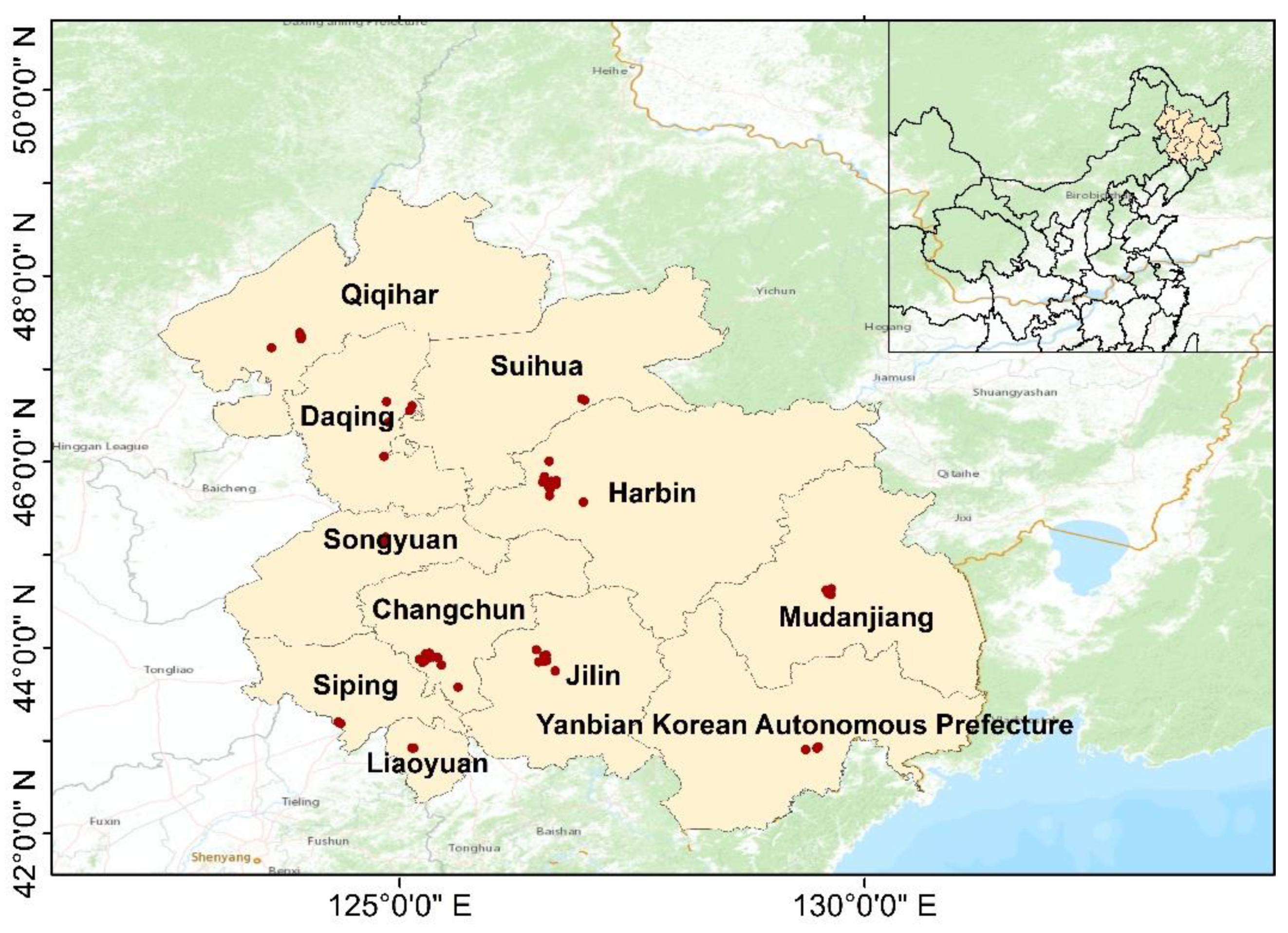
2.1. Research Areas and Data Sources

The research area (Figure 1) includes five cities in Heilongjiang Province (Harbin (HB), Daqing (DQ), Qiqihar (QQH), Suihua (SH), and Mudanjiang (MDJ)) and 6 cities in Jilin Province (Changchun (CC), Jilin (JL), Siping (SP), Liaoyuan (LY), Songyuan (SY), and Yanbian Korean Autonomous Prefecture (YKAP)). The total research area is about 263,600 square kilometers. The southern part of HCUA is the central and southern urban agglomeration of Liaoning Province, the Russian Far East to the north, the Korean Peninsula to the east, and the Inner Mongolia Autonomous Region to the west, echoing the Beijing-Tianjin-Hebei and Bohai Rim areas, which is an important gateway for the opening up of Northeast China. The climatic conditions are subfrigid coniferous climate and monsoon climate of medium latitudes. The precipitation is mainly concentrated in summer, with a large temperature difference between day and night. Four seasons are distinct, and the wintertime is longer [32]. HCUA ranks first among the nine major regional urban agglomerations (national secondary urban agglomeration). Its regional air pollution restricts the green and healthy development of urban agglomerations, which has attracted the attention of all sectors of society.
The concentration data of SO2, NO2, CO, PM10, and PM2.5 used in this paper were hourly monitoring concentration. Because the ozone monitoring concentration fluctuates greatly every hour, the eight-hour moving average were used. The original data were taken from 55 automatic ambient air monitoring stations, which can be downloaded from the website: https://www.mee.gov.cn/ (accessed on 29 June 2021). The data multi-resolution emission inventory (MEIC) of NOx, VOCs (alkanes, alkenes, aromatic hydrocarbons, oxygen-containing VOCs, and nitrogen-containing VOCs), PM, and CO in 2017 were collected from http://meicmodel.org/ (accessed on 29 June 2021). In this study, a year was divided into four quarters: spring (March to May), summer (June to August), autumn (September to November) and winter (December, January, and February). The data of meteorological factors such as temperature (T), wind speed (WS), and sunshine duration (SD) from 2015 to 2019 were obtained from China Meteorological Data Network (http://data.cma.cn/ (accessed on 29 June 2021). For more information on data acquisition, see Table S1.
The raw data were preprocessed to troubleshoot outliers generated by machine faults (including random values generated by monitoring and analysis instrument of substations when it is shut down, random values generated by instrument preheating after substations are reset after power failure, etc.) and ensure data quality, according to the “Monitoring Regulation for Ambient Air Quality” (HJ/T193-2005). The calculation and quantity of valid data meet the relevant requirements of “Ambient Air Quality Standard” (GB3095-2012) and “Technical Specifications for Ambient Air Quality Evaluation (Trial)” (HJ663-2013). According to “Ambient Air Quality Standard”, the daily maximum 8 h average (MDA8) concentration limits of O3 in the first-class and secondary ambient air functional areas are 100 μg/m3 and 160 μg/m3, respectively. Among them, the first-class ambient air functional area refers to areas that need special protection such as nature reserves and scenic spots; secondary ambient air functional areas are residential areas, mixed commercial and transportation areas, cultural areas, industrial areas, and rural areas. Through our analysis, the research area is a secondary ambient air functional area.

2.2. Research Methods

2.2.1. Spatial Autocorrelation Analysis

In this paper, Moran’s I in ArcGIS was used to test the spatial autocorrelation of O3 concentration in the study area. According to the characteristics of the dataset in space, we used the Global Moran’s I tool to determine whether the dataset was disperse, aggregated, or random. The tool calculates the I index value of Moran as well as the Z and P values to further verify the index statistically [33]. The P value represents the probability. The Z score represents a multiple of the standard deviation.
Moran’ I statistics of spatial autocorrelation is expressed in Equation (1):
I = n S 0 i n j n W i j ( x i y ¯ ) ( x j y ¯ ) i n ( x i y ¯ ) 2
Among them,
S 0 = i n j n W i j
In the above formula, n is the total number of elements; x i is the value of independent variable i ; y ¯ is the mean value of dependent variable; W i j is the spatial weight between elements i and j , when two space units are adjacent, W i j = 1 , otherwise W i j = 0 .
Z i score is calculated in Equation (3):
Z i = I E [ I ] V [ I ]
E [ I ] = 1 / ( n 1 )
V [ I ] = E [ I 2 ] E [ I ] 2

2.2.2. Wavelet Analysis of Time Series

In order to reveal the different variation periods in the whole time series and show the change trend of the series on each time scale, the wavelet analysis method was used to analyze the time series of ozone concentration.
The wavelet basis functions is expressed in Equation (6):
ψ a , b ( t ) = | a | 1 / 2 ψ ( t b a )
Among them, a , b R , a 0 In the above formula, ψ a , b ( t ) is the wavelet basis function; a represents the time scale, which reflects the length of the wavelet period; b is the translation parameter, which reflects the passage of the wavelet in time.
The continuous wavelet transform (CWT) is as Equation (7):
W f ( a , b ) = | a | 1 / 2 R f ( t ) ψ ¯ ( t b a ) d t
In the above formula, W f ( a , b ) is the wavelet transform coefficient;   f ( t ) is a finite signal; ψ ¯ ( t b a ) is the complex conjugate function of ( t b a ) .
The wavelet variance is calculate by integrating the square value of the wavelet coefficients in the b domain. The formula is as Equation (8):
Var ( a ) = | W f ( a , b ) | 2 d b
The wavelet variance graph is the curve of the wavelet variance, which is varied with the time scale a. The wavelet variance graph can be used to judge the relative intensity of the time series or signal vibration on different time scales, and the scale a corresponding to the maximum value of variance is the fluctuation period of time series.

3. Results and Discussion

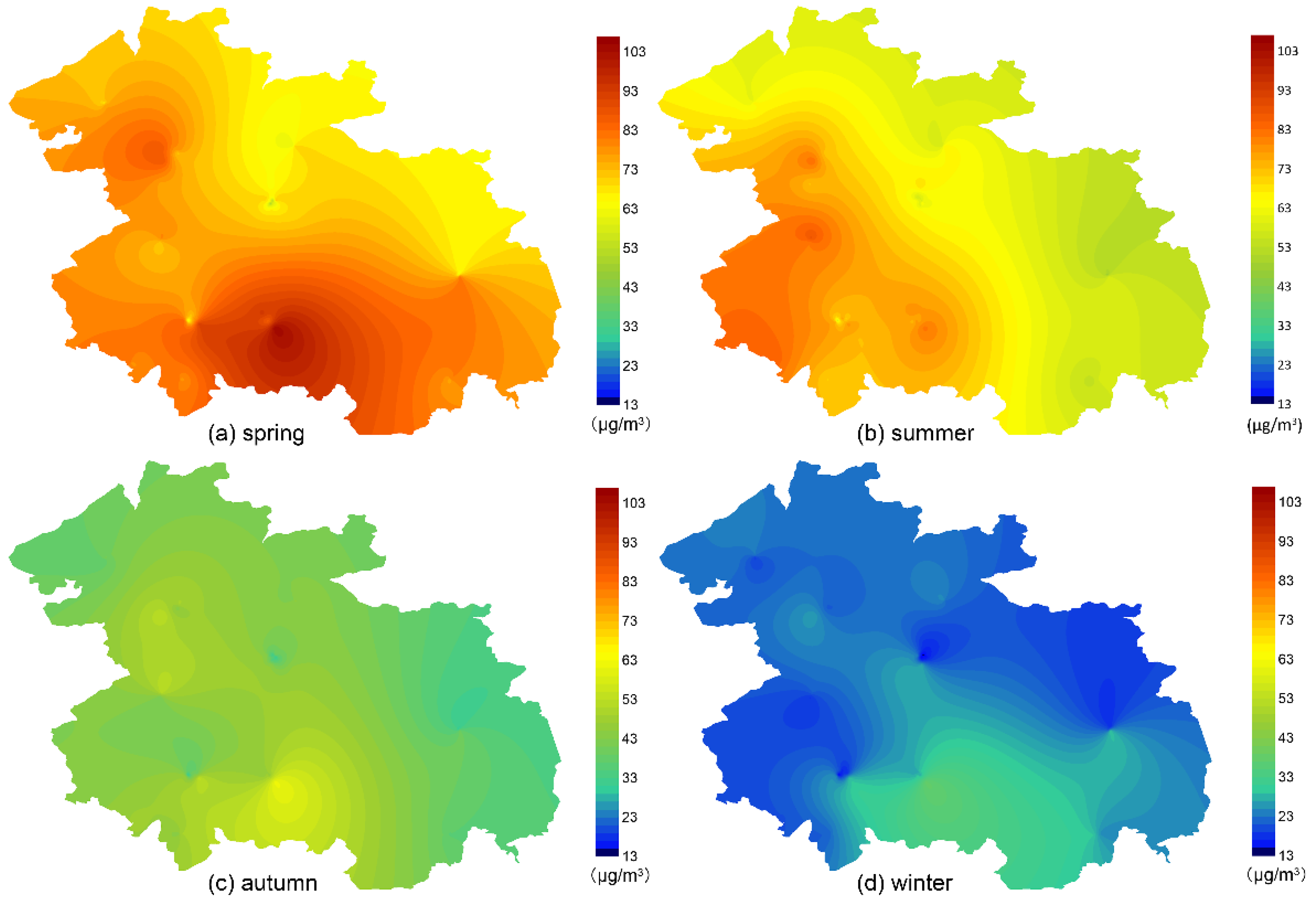
3.1. Spatial Distribution Characteristics of Ozone Concentration

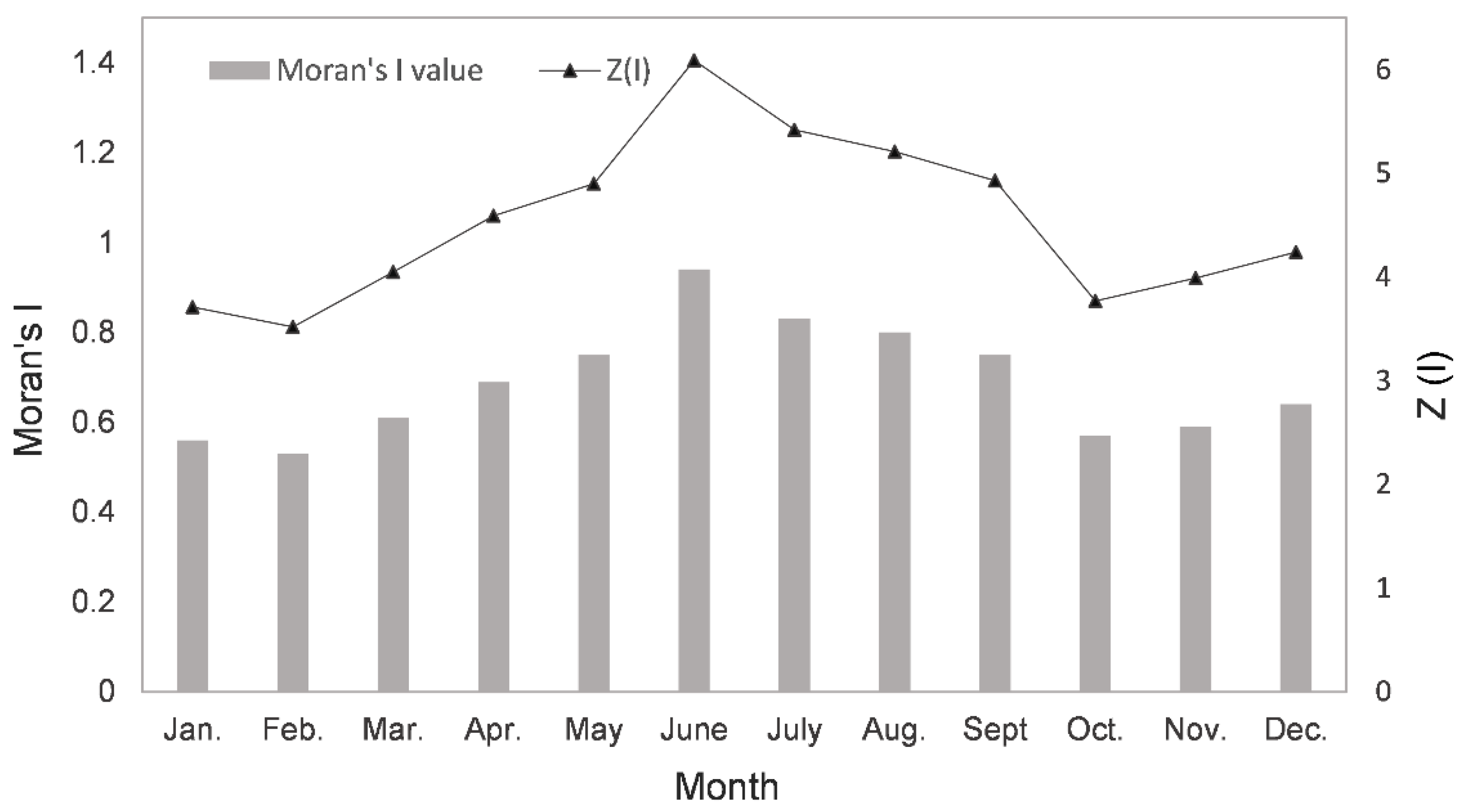
3.1.1. Analysis of Spatial Correlation

The similarity of regional O3 concentration is related to the spatial correlation characteristics of atmospheric activity [34]. Moran’s I index was used to test the spatial correlation of O3 concentration at 55 monitoring stations in HCUA from 2015 to 2019. When Z (I) > +1.65 or <−1.65, and p < 0.1, the confidence coefficient is 90%; when Z (I) > +1.96 or <−1.96 and p < 0.05, the confidence coefficient is 95%; when Z (I) > +2.58 or <−2.58 and p < 0.01, the confidence coefficient is 99%.
For the five-year/seasonal average ozone concentration (Table 1) and monthly average ozone concentration (Table S2, Figure 2), the values of Moran’s I index were all greater than zero, which indicated that there was a positive correlation or high aggregation pattern. By observing the Z(I) and P values, it can be found that the Z score was greater than 2.58, and the p value was less than 0.01, which indicated that the probability (the observed pattern was a random process) was less than 1%. Therefore, the O3 pollution in the study area had a significant positive spatial correlation.
Seasonally, the Moran’s I index in summer was higher than that in other seasons, indicating the spatial accumulation of O3 was the most significant. High concentration areas concentrated in SY and SP, and ozone pollution was relatively stable and persistent. Moran’s I index in winter was lower than that in other seasons, especially in February, and the spatial accumulation of O3 was the most significant. The low concentration area was concentrated in HB, where the ozone concentration was relatively low.

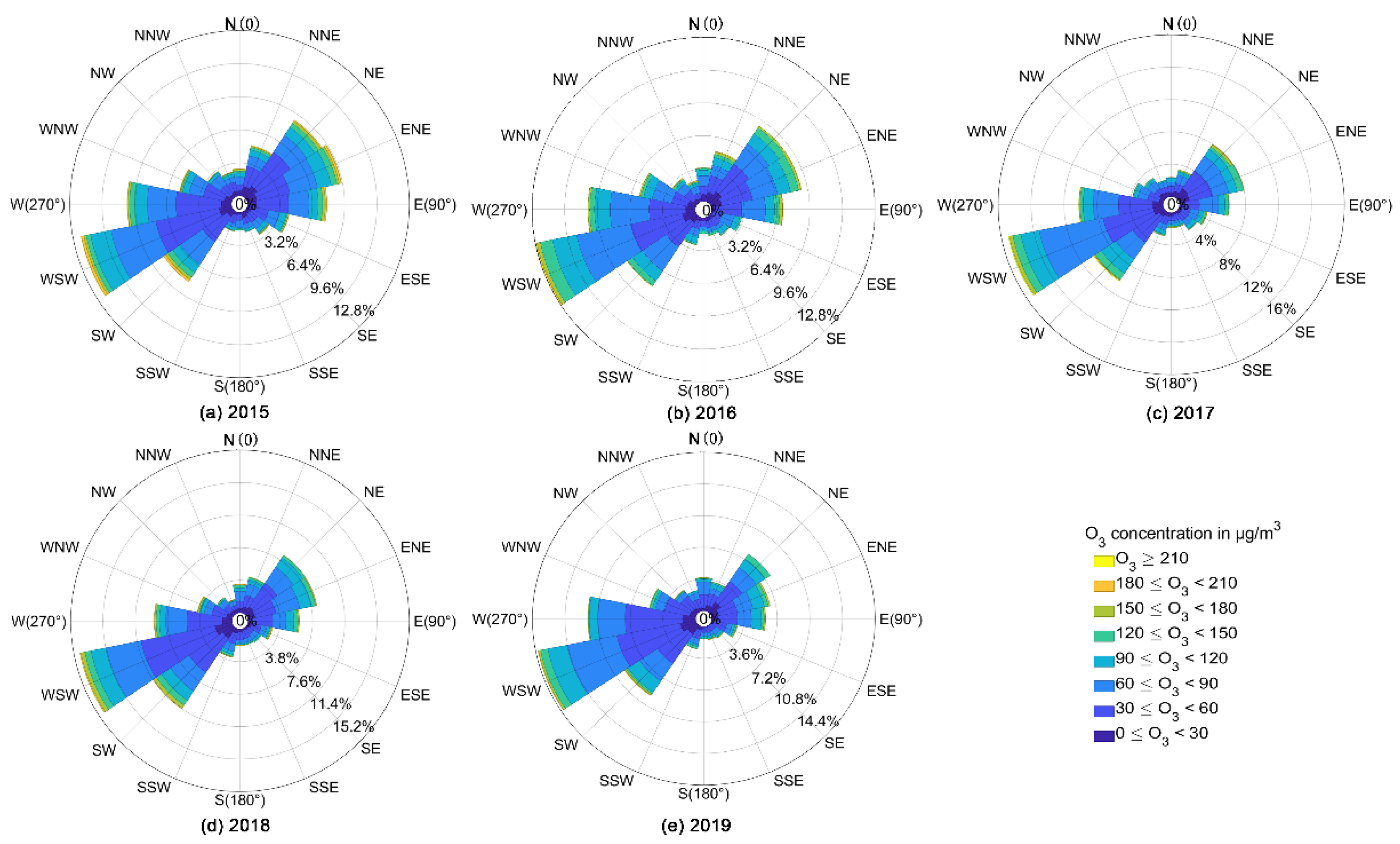
3.1.2. Analysis of the Spatial Distribution

Figure 3 shows the exceed ratio (left) of the daily maximum 8 h O3 average O3 concentration in each monitoring station of HCUA and the spatial distribution characteristics of annual average O3 concentration (right). According to the MDA8 limit of the secondary environmental functional area in the “Ambient Air Quality Standard” (GB3095-2012) (160 μg/m3), the total annual exceeding days of 55 monitoring sites in the study area was 105 days. Among them, the 7 monitoring sites in JL had a relatively high number of days exceeding the standard, with total 45 days, and the 10 monitoring sites in CC had a total of 25 days of exceeding the standard per year. There were no days that exceeded the limit in QQH, SH, MDJ, and YKAP. The distribution of O3 concentration in the study area roughly showed a trend of high concentration in the southern region and low concentration in the northeast, which was consistent with the results of Wei et al. [35]. Among them, JL had the highest annual average concentration of O3 (68.49 μg/m3), followed by DQ (61.92 μg/m3).
VOCs and NOx will undergo photochemical reaction to generate O3 under sufficient light conditions [36,37,38,39]. The studies of ozone generation mechanism based on photochemical model have showed that ozone generation in China’s large cities is mostly in VOCs-controlled areas [40]. According to the statistical results of the 2017 MEIC list in the study region (Table 2), the main source of VOCs in the HCUA was industrial emission sources, which accounted for more than 50% of total emissions. In addition, industrial sources also emitted a mass of NOx and CO. JL, DQ, and CC with high ozone concentration in the study area are all among the top ten heavy industrial cities in Northeast China. Among these cities, JL and DQ are dominated by the petrochemical industry, while CC is dominated by the automobile manufacturing industry. Relatively speaking, the VOCs emissions of these cities would be higher than other cities in the study area.
In addition, related studies showed that relative humidity had a negative effect on O3 concentration. On the one hand, the high humidity environment is conducive to the deposition of O3, and it can reduce O3 concentration in the atmospheric environment [41]; on the other hand, water vapor has an extinction mechanism, which can weaken solar radiation, thus reducing the rate of photochemical reaction [42]. The relative humidity of the study area expresses a trend of high in the northeast and low in the southwest, which is opposite to the distribution of O3 precursors [13]. Under the combined action of the above factors, the annual ozone concentration distribution in the study area showed a pattern of relatively high in the south and low in the northeast.

3.2. Temporal Distribution Characteristics of Ozone Concentration

3.2.1. Analysis of Seasonal Variation

The change trend of O3 concentration between seasons was the following: spring (74.98 μg/m3) > summer (67.95 μg/m3) > autumn (42.14 μg/m3) > winter (21.83 μg/m3). The O3 concentration in winter was significantly lower than other seasons (Figure 4), which was similar to the results already reported [43]. The spatial variation of O3 concentration in spring was characterized by high in the southern region and low concentration in the northeast. In summer, the concentration was high in the southwest and low in the northeast. In autumn and winter, the concentration was higher in the southern and central regions, and lower in other regions.
Igor G. Zurbenko et al. [44] showed that the seasonality of the ozone production rate is directly dependent upon the seasonality of solar radiation. Seasonally, the solar radiation is relatively higher in spring and lowest in winter. High ozone concentration in spring may also be caused by large-scale air mass transport or stratospheric exchange caused by “tropopause folding”. Lv [45] and VanHaver et al. [46] reported that the transport from the stratosphere to the troposphere in the middle and high latitudes is stronger in winter and spring, and weaker in summer and autumn. Oltmans et al. [47] have shown that regular transfer from the stratosphere when ozone concentrations in the lower stratosphere are at their maximum.
In addition, the production of ozone in the troposphere is related to the photochemical process of gases such as carbon monoxide and non-methane hydrocarbons (NMHC) formed in winter [48]. Penkett and Brice [49] found that the peroxyacyl nitrate (PAN) concentration was higher in spring and reached its peak in May. PAN is a clear sign of tropospheric photochemistry. The HCUA is a high latitude area, with short daytime in winter and weak solar radiation. Therefore, although it produces a large amount of NOx and other pollutants for large demand of heating coal and coal-fired power generation, the ozone concentration is low in winter due to the weak photochemical process. Moreover, precursors accumulate in winter, which is conducive to the generation of ozone when solar radiation increases in spring.

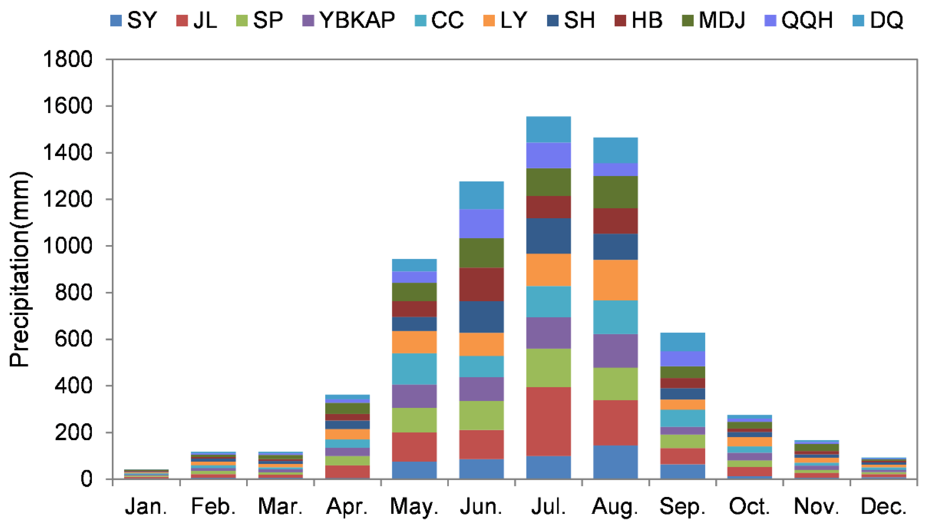
3.2.2. Analysis of Monthly Variation

The change trend of monthly average ozone concentration in the study area can be seen from the stacked graph of hourly values of observed surface O3 (Figure 5). The O3 concentration expressed an upward trend from January to May as the temperature and solar radiation increased. From June to December, the O3 concentration showed a downward trend. Among them, the concentration was relatively high from April to July, and relatively low in January, November, and December. It was consistent with the above seasonal change trend.
The distribution characteristics of monthly rainfall in urban agglomeration were shown in Figure 6. The results show that the rainy season mostly occurs from June to August. During the rainy season, the photochemical reaction in the tropospheric is weakened due to the weakening of the solar radiation flux by the cloud and the direct absorption of ozone and its precursors (NOx, NMHC, etc.) and free radicals (OH, HO2, etc.) by the liquid water in the cloud. After the rainy season, the temperature is low and the light intensity is weak, causing the continuous decrease of O3 concentration [50,51]. In addition, influenced by the geographical location at high latitude, most of the study area started burning coal for heating around November, the increased of anthropogenic emissions lead to the concentration of PM2.5 in the atmosphere increased. It weakened the solar radiation and was not conducive to the formation of ozone. Analyzing the characteristics of daily variation in O3 concentration between different months, it can be found that the typical daytime and night changes of urban areas [52]. The daily high value area appeared approximately 15:00–21:00, and the low value area mostly appeared between 5:00–9:00.

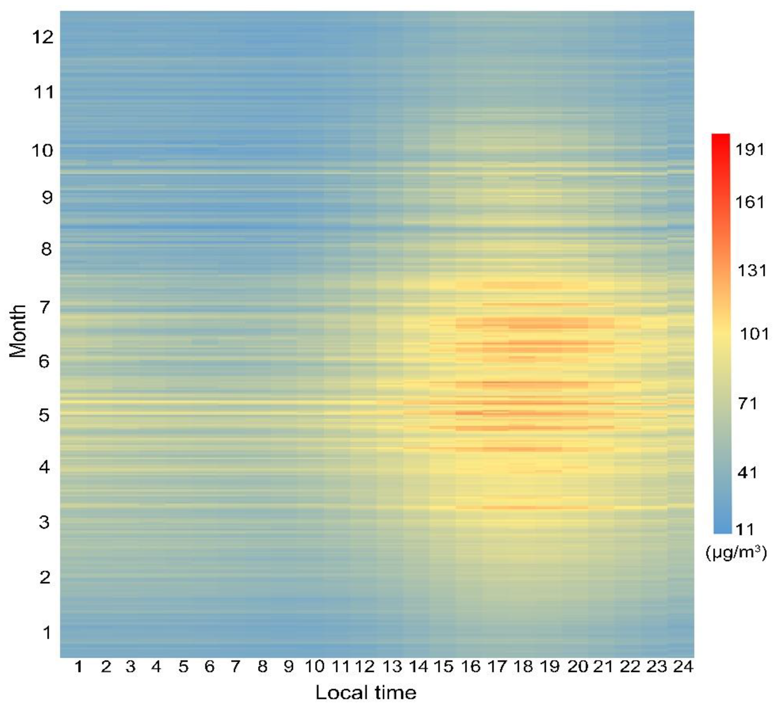
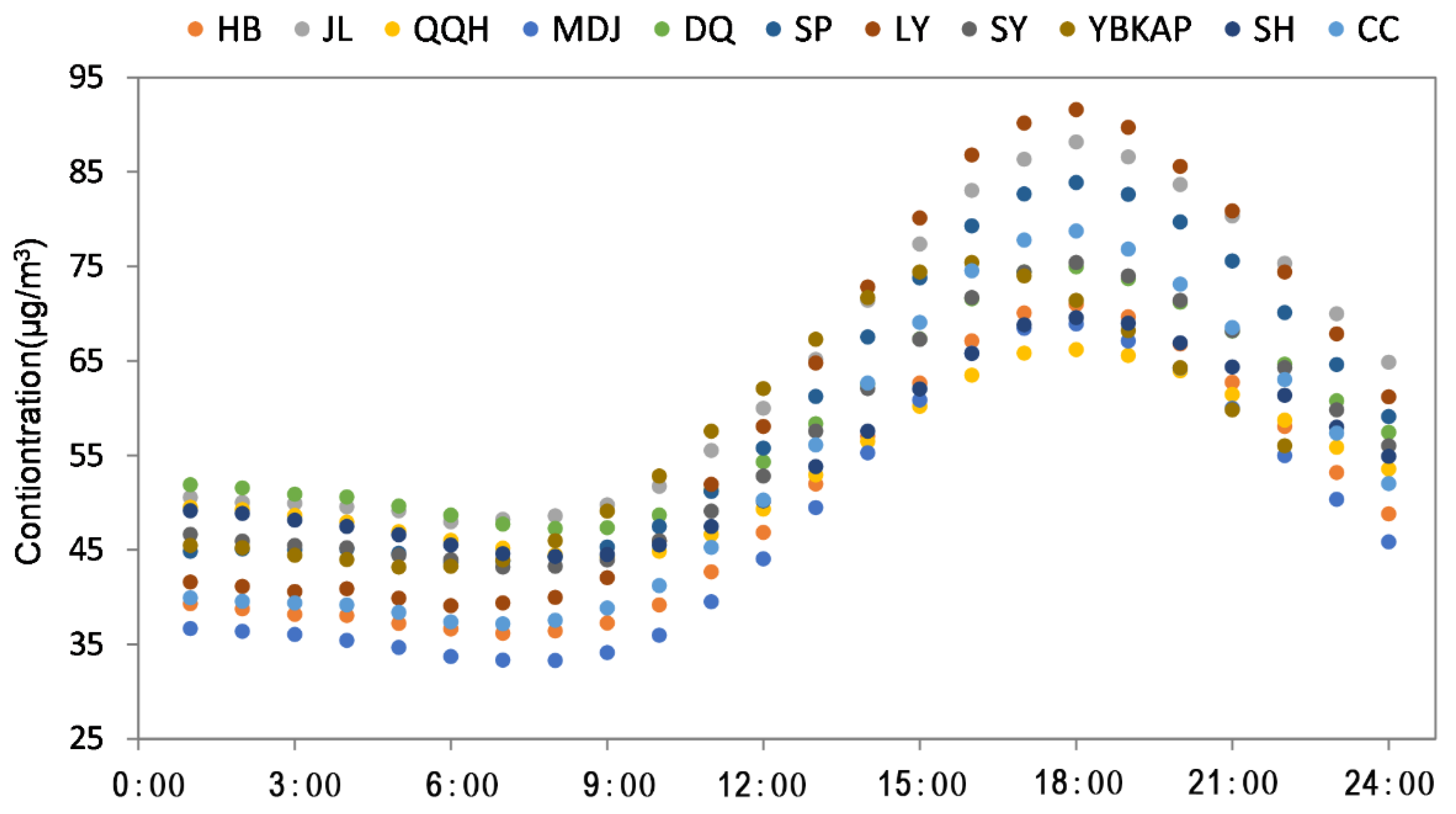
3.2.3. Analysis of the Diurnal Variation

The diurnal variation of O3 concentration among different cities was shown in Figure 7. The results showed that the diurnal variation characteristics of O3 concentration in different cities were similar, which showed a “single peak” pattern. Overall, the O3 concentration showed an upward trend from 9:00 to 18:00, and all 11 cities reached their peak at 18:00. From 18:00 to 7:00 in the next day, the O3 concentration showed a downward trend, and the valleys appeared at 7:00–9:00. The valleys of QQH and SH appeared at 9:00, and the lowest concentrations of SY, YBZ, MDJ, and QQH were at 8:00. The valleys of other cities all appeared at 7:00. Consistent with the results obtained above, the O3 concentration of JL was relatively high in 11 cities, and the concentration of MDJ was relatively low. There was little difference in O3 concentration between different cities.
The diurnal characteristics of O3 concentration may be related to its precursors and solar radiation [53]. Due to the continuous accumulation of O3 precursors (NOx) at night and the emission of traffic sources during the morning peak period, a large number of O3 precursors appeared. With the increasing of daytime light intensity, the photochemical reaction was continuously promoted, so the O3 concentration increased continuously after 7:00-9:00. After 18:00, as the solar radiation weakens, the formation of O3 decreases, and the O3 accumulated near the surface layer is continuously consumed by NO, resulting in a downward trend of O3 concentration.

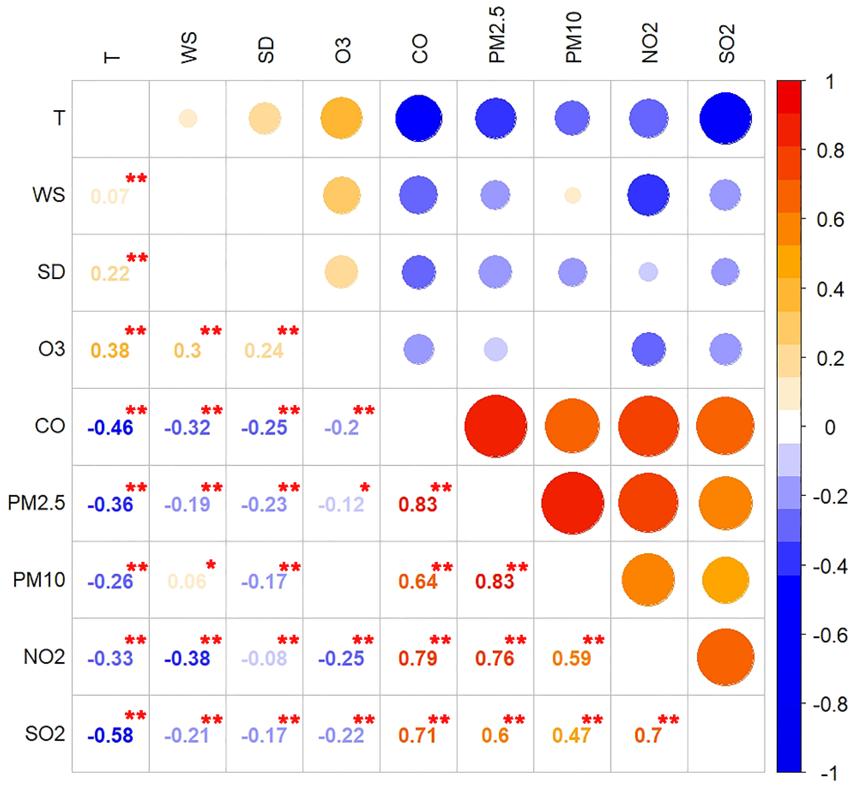
3.3. Analysis of the Correlation between Ozone and Other Pollutants/Meteorological Factors

We select Jilin City (the above analysis showed that the ozone concentration of JL is higher than that of other cities) as the further research area to analyze the correlation between meteorological factors and ozone concentration. In similar studies, Igorg, Zurbenko et al. [44] carried out logarithmic transformation of pollutant concentration to linearize the variable. However, most of the recent studies do not use logarithmic transformation [23,54,55,56,57], and it is considered that there is a linear relationship between pollutant concentration and meteorological factors. We compared the two results. The results showed that the logarithmic transformation had no significant effect on the correlation among the factors (see Tables S3 and S4). Therefore, we used the original concentration of O3 and other pollutants and meteorological data such as wind speed, sunshine duration and temperature for Pearson correlation analysis from 2015 to 2019.
The results of Figure 8 showed that there was a significant positive correlation between O3 concentration and meteorological factors such as T, WS, and SD. Most studies have shown that the main atmospheric factor affecting O3 concentration is solar radiation [19,44,58,59]. Since solar radiation data is difficult to obtain, and some studies have shown that solar radiation and temperature have a significant positive correlation [60,61], therefore, we used T and SD to characterize the effects of solar radiation. The rise of temperature is often accompanied by the increase of solar radiation and the decrease of water vapor, which is beneficial to the natural emission of isoprene. High temperature also leads to the slow release of NOx and associated free radicals by one of the ozone precursors, PAN, leading to high ozone concentration [62].
WS also influence the transport and diffusion of O3. The increase of WS is conducive to the transport of pollutants, and different wind fields will significantly affect the ozone concentration in JL. Figure 9 shows that the prevailing wind direction in the study area has been southwesterly for many years. In 2015, the high concentration of O3 was mainly from the southwest and northeast, while in other years, the high concentration was mainly from the southwest. The O3 concentration in SP and LY in the southwest of JL was relatively high. The O3 and its precursors from the two places may be transported to the study area through the southwest wind, thus increasing the O3 pollution in JL. In addition, related research showed that planetary boundary layer (PBL) is one of the most important metrological elements affecting ozone and other pollution concentrations. Although low PBL has been recognized as a generally good indicator of heavy pollution [63,64], a comparative study of Beijing and Shanghai by Miao et al. [65] showed that the relationship between PBL height and pollution level is variable and complex. Due to the lack of sufficient PBL data in this study, the influence of this parameter on ozone pollution cannot be discussed.
As important precursors of O3 formation, CO and NO2 were negatively correlated with the concentration of O3. In addition, ozone concentration was significantly anticorrelated with PM2.5 concentrations. Under certain conditions, the high concentration of particulate matter would increase the optical thickness of aerosol, which would weaken the photochemical formation rate of ozone and reduce the concentration of O3. Heterogeneous chemical processes occurring on the surface of particulate matter also affect O3 concentrations [66]. The increase in PM2.5 concentrations reduces atmospheric radiation, which restrains O3 levels.

3.4. Time Series of Ozone Concentration

To further analyze the variation cycle and future trend of ozone concentration, Morlet wavelet analysis was conducted on the time series of the average daily ozone concentration in Jilin city in 2019 [67]. The distribution of O3 concentration in the time domain and the periodic variation on each time scale can be seen through the contour map of the real part of wavelet coefficients. The main period of the concentration variation can be found by the wavelet variance graph of the wavelet coefficients of the original time series of the daily average O3 concentration.
Figure 10 shows the multi-time scale characteristics of the average daily ozone concentration in Jilin City. On the whole, the annual ozone concentration showed a trend of alternating cycles, and the distribution strength of each time scale was different. There were obvious periodic variation on time scale a, which was 5–10 days, 15–25 days, and 55–64 days. However, at a scale of 55 to 64 days, the periodic scale was not shown to be complete, so it is not discussed. According to the wavelet coefficient isoline map (Figure 10a), it can be seen that under the scales of 5–10 and 15–25 days, the periodic change of O3 concentration is regional, the isoline and color changes in the early and late stage are not obvious, and the periodicity is strong in the middle stage. The cycle scale of 5–10 days is mainly concentrated between the 120th day and 200th days, that is, between May and July; while the time scale of 15–25 days is mainly concentrated between the 50th day and the 300th day, that is, from March to October.
According to the wavelet square of O3 (Figure 10b), there are two obvious peaks, that is, when a = 9 and a = 23, the wavelet square reaches its maximum value. After the 40th day, the variance increased continuously, but there was no inflection point until the end. The scale of the third period did not show up, which was consistent with the trend shown in the contour map. The time scale of 23 days corresponds to the maximum peak, which was the first main period of the change of O3 concentration, showing the largest time series fluctuation energy and the strongest periodic oscillation. A = 9 was the second main period.
In order to further explore the reasons for the main period of O3 concentration, we analyzed the meteorological factors such as WS, T, SD and precipitation periodically. T and WS showed time-scale variation characteristics similar to ozone, as shown in Figure 10c,d. This is consistent with the results of correlation analysis that O3 concentration was significantly correlated with T and WS. Therefore, the periodic fluctuations of O3 may be related to the above two meteorological factors. In addition, it may be affected by the stability of the boundary layer [68].

4. Conclusions and Suggestions

4.1. Conclusions

In this paper, the temporal and spatial variation characteristics of O3 concentration in important economic cooperation areas in Northeast China were analyzed, aiming to provide some scientific basis for making effective air pollution control plans in the study area and similar urban agglomerations. The results of this paper are as follows:
(1)
The results of Moran’s I index showed that the O3 pollution of HCUA had a significant spatial positive correlation. Affected by solar radiation, relative humidity and emissions from industrial and traffic sources, the spatial distribution of O3 concentration in the study area was generally higher in the south and lower in the northeast.
(2)
The difference of regional O3 concentration between different seasons was mainly affected by meteorological conditions, which was as follows: spring > summer > autumn > winter. Higher concentrations of near-surface ozone in spring may be related to high solar radiation, air quality transport caused by tropopause folding and photochemical process of gases pollutants such as carbon monoxide. The diurnal variation characteristics of O3 concentration in different cities were similar, showed a “single peak” pattern. The valley value appeared between 7:00 and 9:00, and the peak value appeared at 18:00.
(3)
The results of correlation analysis showed that there was a significant negative correlation between O3 concentration and CO, NO2, SO2, and PM2.5 concentration. The effects of solar radiation intensity, water vapor, isoprene, and ozone precursors on the process of ozone formation resulted in a significant positive correlation between ozone concentration and temperature and sunshine duration. In addition, the wind speed also had an impact on the transfer of ozone, and correlation between the wind speed and ozone was positively correlated.
(4)
The continuous wavelet transform analysis of the time series of ozone concentration in Jilin City showed that there was a significant periodic fluctuation of ozone in the time scale of a = 9,23. This periodic fluctuation was particularly evident from May to July, and temperature and wind speed showed similar time-scale variation characteristics with O3, indicating that them had a great influence on the periodic variation of O3. In addition, its periodicity may be related to the stability of boundary layer, horizontal advection, and other factors.

4.2. Suggestions

Pollution control is based on an exhaustive understanding of pollutant characteristics. Harbin-Changzhou City Agglomeration is dominated by equipment manufacturing, engineering machinery, machine tools, metallurgy, petrochemical, and other industries, which emit a large number of VOCs and other ozone precursors in the production process. In addition, results of the source emission inventory show that the precursors in the study area are mostly emitted by industry. The industrial distribution has a great influence on the ozone concentration. Therefore, industrial structure adjustment and upgrading to effectively reduce the emission of ozone precursors in the study area will help to decrease ozone concentration. Studies show that the generation of O3 is not only related to the emissions of precursor VOCs and NOx but also closely related to the proportion between two precursors, which show a complex nonlinear response relationship [69]. It is also the key to further exploring the influence of the proportion of regional precursor VOCs and NOx on O3 concentration for controlling ozone pollution. In addition, the spatial distribution of O3 concentration indicates that the pollution has regional characteristics. Therefore, the construction of trans-regional ozone pollution control system to prevent the regional composite pollution of various pollutants, focusing on the prevention and control of volatile organic compounds, nitrogen oxides, and other precursors with strong mobility, will also be conducive to the treatment of ozone and other pollutants.

Supplementary Materials

The following are available online at https://www.mdpi.com/article/10.3390/atmos12070843/s1. Table S1. Data sources of pollutants and meteorological factors; Table S2. Spatial autocorrelation value of ozone month average concentration in Harbin Changchun urban agglomeration, 2015-2019; Table S3. Correlation coefficients between O3 and meteorological elements/other pollutants (No logarithmic transformation); Table S4. Correlation coefficients between O3 and meteorological elements/other pollutants (logarithmic transformation).

Author Contributions

Conceptualization, J.T.; data curation, C.F.; formal analysis, J.Q.; methodology, C.F.; supervision, J.W.; writing—original draft, J.T.; writing—review and editing, J.T. All authors read and approved the final submitted manuscript.

Funding

This research was funded by Ecology and Environment Department of Jilin Province. The project numbers are 2018-19 and 2019-08.

Institutional Review Board Statement

Not applicable.

Informed Consent Statement

Not applicable.

Data Availability Statement

The datasets supporting the conclusions of this article are included within the article and its additional file.

Acknowledgments

The authors would like to thank the group members of Laboratory 537 and 142 of Jilin University.

Conflicts of Interest

The authors declare no conflict of interest.

References

  1. Lehman, J.; Swinton, K.; Bortnick, S.; Hamilton, C.; Baldridge, E.; Eder, B.; Cox, B. Spatio-temporal characterization of tropospheric ozone across the eastern United States. Atmos. Environ. 2004, 38, 4357–4369. [Google Scholar] [CrossRef]
  2. Pan, G.; Pan, Q.; Zhang, G. The harm of Ozone pollution and the significance of Ozone Monitoring. In Proceedings of the 2013 Annual meeting of the Chinese Society of Environmental Science, Kunming, China, 8 March 2013; p. 5. [Google Scholar]
  3. Post, E.S.; Grambsch, A.; Weaver, C.; Morefield, P.; Huang, J.; Leung, L.Y.; Nolte, C.G.; Adams, P.; Liang, X.Z.; Zhu, J.H.; et al. Variation in estimated ozone-related health impacts of climate change due to modeling choices and assumptions. Environ. Health Perspect. 2012, 120, 1559–1564. [Google Scholar] [CrossRef] [PubMed]
  4. Mills, G.; Harmens, H.; Wagg, S.; Sharps, K.; Hayes, F.; Fowler, D.; Sutton, M.; Davies, B. Ozone impacts on vegetation in a nitrogen enriched and changing climate. Environ. Pollut. 2016, 208, 898–908. [Google Scholar] [CrossRef] [PubMed] [Green Version]
  5. Li, Y.; Shang, Y.; Zheng, C.; Ma, Z. Estimated Acute Effects of Ozone on Mortality in a Rural District of Beijing, China, 2005–2013: A Time-Stratified Case-Crossover Study. Int. J. Environ. Res. Public Health 2018, 15, 2460. [Google Scholar] [CrossRef] [PubMed] [Green Version]
  6. Tao, Y.; Huang, W.; Huang, X.; Zhong, L.; Lu, S.-E.; Li, Y.; Dai, L.; Zhang, Y.; Zhu, T. Estimated acute effects of ambient ozone and nitrogen dioxide on mortality in the Pearl River Delta of southern China. Environ. Health Perspect. 2012, 120, 393–398. [Google Scholar] [CrossRef]
  7. Aris, R.M.; Christian, D.; Hearne, P.Q.; Kerr, K.; Finkbeiner, W.E.; Balmes, J.R. Ozone-induced Airway Inflammation in Human Subjects as Determined by Airway Lavage and Biopsy. Am. Rev. Respir. Dis. 1993, 148, 1363–1372. [Google Scholar] [CrossRef]
  8. Shang, Y.; Sun, Z.; Cao, J.; Wang, X.; Zhong, L.; Bi, X.; Li, H.; Liu, W.; Zhu, T.; Huang, W. Systematic review of Chinese studies of short-term exposure to air pollution and daily mortality. Environ. Int. 2013, 54, 100–111. [Google Scholar] [CrossRef]
  9. Feng, Z.; Kobayashi, K. Assessing the impacts of current and future concentrations of surface ozone on crop yield with meta-analysis. Atmos. Environ. 2008, 43, 1510–1519. [Google Scholar] [CrossRef]
  10. Geng, C.; Wang, Z.; Ren, L.; Wang, Y.; Wang, Q.; Yang, W.; Bai, Z. Study on the Impact of Elevated Atmospheric Ozone on Crop Yield. Res. Environ. Sci. 2014, 27, 239–245. [Google Scholar]
  11. Li, Q.; Wang, E.; Zhang, T.; Hu, H. Spatial and Temporal Patterns of Air Pollution in Chinese Cities. Water Air Soil Pollut. 2017, 228, 1–22. [Google Scholar] [CrossRef]
  12. Cheng, L.; Wang, S.; Gong, Z.; Li, H.; Yang, Q.; Wang, Y. Regionalization based on spatial and seasonal variation in ground-level ozone concentrations across China. J. Environ. Sci. 2018, 67, 179–190. [Google Scholar] [CrossRef] [Green Version]
  13. Chen, Z.; Shao, T.; Zhao, J.; Cao, J.; Yue, D. Evolution Law and influencing factors of Spatial pattern of Ozone concentration in Northeast China. Acta Sci. Circumstantiae 2020, 40, 3071–3080. [Google Scholar]
  14. Cardelino, C.A.; Chameides, W.L. An observation-based model for analyzing ozone precursor relationships in the urban atmosphere. J. Air Waste Manag. Assoc. 1995, 45, 161–180. [Google Scholar] [CrossRef] [PubMed]
  15. Zhang, Y.; Wang, W.; Wu, S.-Y.; Wang, K.; Minoura, H.; Wang, Z. Impacts of updated emission inventories on source apportionment of fine particle and ozone over the southeastern U.S. Atmos. Environ. 2014, 88, 133–154. [Google Scholar] [CrossRef]
  16. Guo, H.; Chen, K.; Wang, P.; Hu, J.; Ying, Q.; Gao, A.; Zhang, H. Simulation of summer ozone and its sensitivity to emission changes in China. Atmos. Pollut. Res. 2019, 10, 1543–1552. [Google Scholar] [CrossRef]
  17. Cao, T.; Wu, K.; Kang, P.; Wen, X.; Li, H.; Wang, Y.; Lu, X.; Li, A.; Pan, W.; Fan, W.; et al. Study on ozone pollution characteristics and meteorological cause of Chengdu-Chongqing urban agglomeration. Acta Sci. Circumstantiae 2018, 38, 1275–1284. [Google Scholar]
  18. Ding, A.J.; Fu, C.B.; Yang, X.Q.; Sun, J.N.; Zheng, L.F.; Xie, Y.N.; Herrmann, E.; Nie, W.; Petäjä, T.; Kerminen, V.M.; et al. Ozone and fine particle in the western Yangtze River Delta: An overview of 1 yr data at the SORPES station. Atmos. Chem. Phys. 2013, 13, 5813–5830. [Google Scholar] [CrossRef] [Green Version]
  19. Fang, C.; Wang, L.; Wang, J. Analysis of the Spatial-Temporal Variation of the Surface Ozone Concentration and Its Associated Meteorological Factors in Changchun. Environments 2019, 6, 46. [Google Scholar] [CrossRef] [Green Version]
  20. Toh, Y.Y.; Lim, S.F.; Glasow, R.V. The influence of meteorological factors and biomass burning on surface ozone concentrations at Tanah Rata, Malaysia. Atmos. Environ. 2013, 70, 435–446. [Google Scholar] [CrossRef]
  21. Silver, B.; Reddington, C.L.; Arnold, S.R.; Spracklen, D.V. Substantial changes in air pollution across China during 2015–2017. Environ. Res. Lett. 2018, 13, 114012. [Google Scholar] [CrossRef]
  22. Wang, T.; Xue, L.; Brimblecombe, P.; Lam, Y.F.; Li, L.; Zhang, L. Ozone pollution in China: A review of concentrations, meteorological influences, chemical precursors, and effects. Sci. Total Environ. 2017, 575, 1582–1596. [Google Scholar] [CrossRef] [PubMed]
  23. Yin, C.Q.; Solmon, F.; Deng, X.J.; Zou, Y.; Deng, T.; Wang, N.; Li, F.; Mai, B.R.; Liu, L. Geographical distribution of ozone seasonality over China. Sci. Total Environ. 2019, 689, 625–633. [Google Scholar] [CrossRef] [PubMed]
  24. Shi, C.; Wang, S.; Liu, R.; Zhou, R.; Li, D.; Wang, W.; Li, Z.; Cheng, T.; Zhou, B. A study of aerosol optical properties during ozone pollution episodes in 2013 over Shanghai, China. Atmos. Res. 2015, 153, 235–249. [Google Scholar] [CrossRef]
  25. Wang, W.; Cheng, T.; Gu, X.; Chen, H.; Guo, H.; Wang, Y.; Bao, F.; Shi, S.; Xu, B.; Zuo, X.; et al. Assessing Spatial and Temporal Patterns of Observed Ground-level Ozone in China. Sci. Rep. 2017, 7, 1–2. [Google Scholar] [CrossRef]
  26. Lu, K.; Zhang, Y.; Su, H.; Shao, M.; Zeng, L.; Zhong, L.; Xiang, Y.; Chang, C.; Chou, C.K.C.; Wahner, A. Regional ozone pollution and key controlling factors of photochemical ozone production in Pearl River Delta during summer time. Sci. China Chem. 2010, 53, 651–663. [Google Scholar] [CrossRef]
  27. Li, B.; Shi, X.; Liu, Y.; Lu, L.; Wang, G.; Thapa, S.; Sun, X.; Fu, D.; Wang, K.; Qi, H. Long-term characteristics of criteria air pollutants in megacities of Harbin-Changchun megalopolis, Northeast China: Spatiotemporal variations, source analysis, and meteorological effects. Environ. Pollut. 2020, 267, 115441. [Google Scholar] [CrossRef] [PubMed]
  28. Li, C.; Yuan, Z.; Wu, Y.; Ban, W.; Li, D.; Ji, C.; Gao, W. Analysis of Persistence and Intensification Mechanism of a Heavy Haze Event in Shenyang. Res. Environ. Sci. 2017, 30, 349–358. [Google Scholar]
  29. Kang, H.; Liu, Y.; Li, T. Characteristics of Air Quality Index and Its Relationship with Meteorological Factors in Key Cities of Heilongjiang Province. J. Nat. Resour. 2017, 32, 692–703. [Google Scholar]
  30. Chen, W.; Liu, Y.; Wu, X.; Bao, Q.; Gao, Z.; Zhang, X.; Zhao, H.; Zhang, S.; Xiu, A.; Chen, T. Spatial and Temporal Characteristics of Air Quality and Cause Analysis of Heavy Pollution in Northeast China. Environ. Sci. 2019, 40, 4810–4823. [Google Scholar]
  31. Heather, S.; Adam, R.; Benjamin, W.; Jia, X.; Neil, F. Ozone trends across the United States over a period of decreasing NOx and VOC emissions. Environ. Sci. Technol. 2015, 49, 186–195. [Google Scholar]
  32. Guo, R.; Wu, T.; Liu, M.; Huang, M.; Stendardo, L.; Zhang, Y. The Construction and Optimization of Ecological Security Pattern in the Harbin-Changchun Urban Agglomeration, China. Int. J. Environ. Res. Public Health 2019, 16, 1190. [Google Scholar] [CrossRef] [PubMed] [Green Version]
  33. Kumari, M.; Sarma, K.; Sharma, R. Using Moran’s I and GIS to study the spatial pattern of land surface temperature in relation to land use/cover around a thermal power plant in Singrauli district, Madhya Pradesh, India. Remote Sens. Appl. Soc. Environ. 2019, 15, 100239. [Google Scholar] [CrossRef]
  34. Wang, Z.; Fang, C.; Xu, G.; Pan, Y. The Spatio-temporal variation of PM2.5 concentration in Chinese cities in 2014. Acta Geogr. Sin. 2015, 70, 1720–1734. [Google Scholar]
  35. Wei, P.; Shao, T.; Huang, X.; Zhang, Z. Study on Spatio-temporal variation characteristics and driving factors of Ozone concentration in Northeast China from 2015 to 2018. J. Ecol. Rural Environ. 2020, 36, 988–997. [Google Scholar]
  36. Atkinson, R. Atmospheric chemistry of VOCs and NOx. Atmos. Environ. 2000, 34, 2063–2101. [Google Scholar] [CrossRef]
  37. Duan, J.; Tan, J.; Yang, L.; Wu, S.; Hao, J. Concentration, sources and ozone formation potential of volatile organic compounds (VOCs) during ozone episode in Beijing. Atmos. Res. 2008, 88, 25–35. [Google Scholar] [CrossRef]
  38. Finlayson-Pitts, B.J.; Pitts, J.N., Jr. Tropospheric air pollution: Ozone, airborne toxics, polycyclic aromatic hydrocarbons, and particles. Science 1997, 276, 1045–1052. [Google Scholar] [CrossRef] [Green Version]
  39. An, J. Plant Volatile Or Ganic Compounds VOCs in Ozone Polluted Atmospheres: The Ecological; Nanjing University of Information Science & Technology: Nanjing, China, 2007. [Google Scholar]
  40. Jiang, M.; Lu, K.; Su, R.; Tan, Z.; Wang, H.; Li, L.; Fu, Q.; Zhai, C.; Tan, Q.; Yue, D.; et al. Ozone formation and key VOCs in typical Chinese city clusters. Chin. Sci. Bull. 2018, 63, 1130–1141. [Google Scholar] [CrossRef]
  41. Kavassalis, S.C.; Murphy, J.G. Understanding ozone-meteorology correlations: A role for dry deposition. Geophys. Res. Lett. 2017, 44, 2922–2931. [Google Scholar] [CrossRef]
  42. Jacob, D.J.; Winner, D.A. Effect of climate change on air quality. Atmos. Environ. 2009, 43, 51–63. [Google Scholar] [CrossRef] [Green Version]
  43. Vingarzan, R. A review of surface ozone background levels and trends. Atmos. Environ. 2004, 38, 3431–3442. [Google Scholar] [CrossRef]
  44. Tsakiri, K.G.; Zurbenko, I.G. Determining the main atmospheric factor on ozone concentrations. Meteorol. Atmos. Phys. 2010, 109, 129–137. [Google Scholar] [CrossRef]
  45. Jian, Y.; daren, L. Diagnosed Seasonal Variation of Stratosphere-Troposphere Exchange in the Northern Hemisphere by 2000 Data. Chin. J. Atmos. Sci. 2004, 28, 294–300. [Google Scholar]
  46. Haver, P.V.; Muer, D.D.; Beekmann, M.; Mancier, C. Climatology of tropopause folds at midlatitudes. Geophys. Res. Lett. 1996, 23, 1033–1036. [Google Scholar] [CrossRef]
  47. Oltmans, S.J.; Levy, H. Surface ozone measurements from a global network. Atmos. Environ. 1994, 28, 9–24. [Google Scholar] [CrossRef]
  48. Penkett, S.A.; Blake, N.J.; Lightman, P.; Marsh, A.R.W.; Anwyl, P.; Butcher, G. The Seasonal Variation of Nonmethane Hydrocarbons in the Free Troposphere Over the North Atlantic Ocean: Possible Evidence for Extensive Reaction of Hydrocarbons With the Nitrate Radical. J. Geophys. Res. Atmos. 1993, 98, 2865–2885. [Google Scholar] [CrossRef]
  49. Penkett, S.A.; Brice, K.A. The spring maximum in photo-oxidants in the Northern Hemisphere troposphere. Nature 1986, 319, 655–657. [Google Scholar] [CrossRef]
  50. Li, R.; Wang, Z.; Cui, L.; Fu, H.; Zhang, L.; Kong, L.; Chen, W.; Chen, J. Air pollution characteristics in China during 2015–2016: Spatiotemporal variations and key meteorological factors. Sci. Total Environ. 2019, 648, 902–915. [Google Scholar] [CrossRef] [PubMed]
  51. Tai, A.P.K.; Mickley, L.J.; Jacob, D.J. Correlations between fine particulate matter (PM2.5) and meteorological variables in the United States: Implications for the sensitivity of PM2.5 to climate change. Atmos. Environ. 2010, 44, 3976–3984. [Google Scholar] [CrossRef]
  52. Lal, S.; Naja, M.; Subbaraya, B.H. Seasonal variations in surface ozone and its precursors over an urban site in India. Atmos. Environ. 2000, 34, 2713–2724. [Google Scholar] [CrossRef]
  53. Abdul-Wahab, S.; Bouhamra, W.; Ettouney, H.; Sowerby, B.; Crittenden, B.D. Predicting ozone levels: A statistical model for predicting ozone levels in the Shuaiba Industrial Area, Kuwait. Environ. Sci. Pollut. Res. Int. 1996, 3, 195–204. [Google Scholar] [CrossRef]
  54. Doğan, B.; Jebli, M.B.; Shahzad, K.; Farooq, T.H.; Shahzad, U. Investigating the Effects of Meteorological Parameters on COVID-19: Case Study of New Jersey, United States. Environ. Res. 2020, 191, 110148. [Google Scholar] [CrossRef] [PubMed]
  55. Alexandrino, K.; Zalakeviciute, R.; Viteri, F. Seasonal variation of the criteria air pollutants concentration in an urban area of a high-altitude city. Int. J. Environ. Sci. Technol. 2021, 18, 1167–1180. [Google Scholar] [CrossRef]
  56. Zexia, D.; Yuanjian, Y.; Linlin, W.; Changwei, L.; Sihui, F.; Chen, C.; Yingxiang, T.; Xinfeng, L.; Zhiqiu, G. Temporal characteristics of carbon dioxide and ozone over a rural-cropland area in the Yangtze River Delta of eastern China. Sci. Total Environ. 2021, 757, 143750. [Google Scholar]
  57. Kliengchuay, W.; Worakhunpiset, S.; Limpanont, Y.; Meeyai, A.C.; Tantrakarnapa, K. Influence of the meteorological conditions and some pollutants on PM210 concentrations in Lamphun, Thailand. J. Environ. Health Sci. Eng. 2021, 19, 237–249. [Google Scholar] [CrossRef] [PubMed]
  58. Ordóñez, C.; Garrido-Perez, J.M.; García-Herrera, R. Early spring near-surface ozone in Europe during the COVID-19 shutdown: Meteorological effects outweigh emission changes. Sci. Total Environ. 2020, 747, 141322. [Google Scholar] [CrossRef] [PubMed]
  59. Jiawei, X.; Xin, H.; Nan, W.; Yuanyuan, L.; Aijun, D. Understanding ozone pollution in the Yangtze River Delta of eastern China from the perspective of diurnal cycles. Sci. Total Environ. 2021, 752, 141928. [Google Scholar]
  60. Shen, Y.; Wang, B. Effect of surface solar radiation variations on temperature in South-East China during recent 50 years. Chin. J. Geophys. 2011, 54, 1457–1465. [Google Scholar]
  61. Daut, I.; Yusoff, M.I.; Ibrahim, S.; Irwanto, M.; Nsurface, G. Relationship between the Solar Radiation and Surface Temperature in Perlis. In Advanced Materials Research; Trans Tech Publications Ltd.: Baech, Switzerland, 2012. [Google Scholar]
  62. Kotchenruther, R.A.; Jaffe, D.A.; Jaeglé, L. Ozone photochemistry and the role of peroxyacetyl nitrate in the springtime northeastern Pacific troposphere: Results from the Photochemical Ozone Budget of the Eastern North Pacific Atmosphere (PHOBEA) campaign. J. Geophys. Res. 2001, 106, 28731–28742. [Google Scholar] [CrossRef] [Green Version]
  63. Zhong, J.; Zhang, X.; Dong, Y.; Wang, Y.; Liu, C.; Wang, J.; Zhang, Y.; Che, H. Feedback effects of boundary_layer meteorological factors on cumulative explosive growth of PM2.5 during winter heavy pollution episodes in Beijing from 2013 to 2016. Atmos. Chem. Phys. 2018, 18, 247–258. [Google Scholar] [CrossRef] [Green Version]
  64. Miao, Y.; Liu, S.; Guo, J.; Huang, S.; Yan, Y.; Lou, M. Unraveling the relationships between boundary layer height and PM2.5 pollution in China based on four_year radiosonde measurements. Environ. Pollut. 2018, 243, 1186–1195. [Google Scholar] [CrossRef] [PubMed]
  65. Miao, Y.; Che, H.; Zhang, X.; Liu, S. Relationship between summertime concurring PM2.5 and O3 pollution and boundary layer height differs between Beijing and Shanghai, China. Environ. Pollut. 2020, 115775. [Google Scholar] [CrossRef] [PubMed]
  66. Cai, Y. Observation and Numerical Modeling on the Interaction between Atmospheric Particulate and Ozone in Urban Area of Yangtze River Delta; Nanjing University: Nanjing, China, 2012. [Google Scholar]
  67. Wang, M. Analysis of Spatio-Temporal Distribution Characteristics and Related Factors of Atmospheric PM2.5 in Shanghai; Shanghai Jiaotong University: Shanghai, China, 2017. [Google Scholar]
  68. Zeri, M.; Carvalho, V.S.B.; Cunha-Zeri, G.; Oliveira-Júnior, J.F.; Lyra, G.B.; Freitas, E.D. Assessment of the variability of pollutants concentration over the metropolitan area of São Paulo, Brazil, using the wavelet transform. Atmos. Sci. Lett. 2016, 17, 87–95. [Google Scholar] [CrossRef] [Green Version]
  69. Cui, M.; An, X.; Xing, L.; Li, G.; Tang, G.; He, J.; Long, X.; Zhao, S. Simulated Sensitivity of Ozone Generation to Precursors in Beijing during a High O 3 Episode. Adv. Atmos. Sci. 2021, 38, 1223–1237. [Google Scholar] [CrossRef]
Figure 1. Air quality monitoring stations in HCUA.
Atmosphere 12 00843 g001
Figure 2. Spatial autocorrelation value of ozone monthly average concentration of HCUA.
Atmosphere 12 00843 g002
Figure 3. Percentage excess of the MDA8 O3 concentration above the standard on five-year basis (left) and Spatial distribution of five-year average O3 concentration in HCUA, 2015–2019 (right).
Atmosphere 12 00843 g003
Figure 4. Spatial distribution of seasonal average concentration of O3.
Atmosphere 12 00843 g004
Figure 5. The stacked graph of hourly values of observed surface O3 from 2015 to 2019.
Atmosphere 12 00843 g005
Figure 6. Monthly rainfall distribution in HCUA.
Atmosphere 12 00843 g006
Figure 7. Hourly O3 concentration from 2015 to 2019.
Atmosphere 12 00843 g007
Figure 8. Correlation coefficients between O3 and meteorological elements/other pollutants. (** indicates that the correlation is significant at level 0.01 (double tail). * indicates that the correlation is significant at level 0.05 (double tail)).
Atmosphere 12 00843 g008
Figure 9. O3 concentration rose map of Jilin from 2015 to 2019.
Atmosphere 12 00843 g009
Figure 10. Real-part contours of wavelet coefficients (a), wavelet coefficient squared figure of O3 (b), wavelet coefficient squared figure of T (c), and wavelet coefficient squared figure of WS (d).
Atmosphere 12 00843 g010
Table 1. Spatial autocorrelation value of ozone five-year/seasonal average concentration in HCUA, 2015–2019.
TimeYearSpr.SumAut.Win.
Moran’s I0.750.700.910.660.59
Z(I)4.934.595.904.343.92
P(10−5)0.10.401.59
Table 2. The total emission of VOCs, NOx, PM2.5, PM10, SO2, and CO in HCUA during 2017.
VOCsSO2NOxPM2.5PM10CO
Industry86.5624.5862.1214.757.84172.69
Power0.265.4922.292.491.7816.72
Residential49.6916.6312.7334.054.67674.75
Transportation19.351.6742.412.960.07114.90
Publisher’s Note: MDPI stays neutral with regard to jurisdictional claims in published maps and institutional affiliations.

