Article

Black Carbon Emissions from the Siberian Fires 2019: Modelling of the Atmospheric Transport and Possible Impact on the Radiation Balance in the Arctic Region

by
Sergey Kostrykin
1,2,3,*,
Anastasia Revokatova
1,4,*,
Alexey Chernenkov
5,
Veronika Ginzburg
1,6,*,
Polina Polumieva
1 and
Maria Zelenova
1
1
Israel Institute of Global Climate and Ecology, Glebovskaya 20B, 107258 Moscow, Russia
2
Marchuk Institute of Numerical Mathematics of the Russian Academy of Sciences, Gubkina Str., 8, 119333 Moscow, Russia
3
Obukhov Institute of Atmospheric Physics of the Russian Academy of Sciences, Pyzhyovskiy per., 3, 119017 Moscow, Russia
4
Hydrometeorological Research Center of the Russian Federation, Bolshoi Predtechensky per. 11-13, 123242 Moscow, Russia
5
Moscow Institute of Physics and Technology, Institutskiy per. 9, Dolgoprudny, 141701 Moscow, Russia
6
Institute of Geography Russian Academy of Science, Staromonetny Line, 29, 119017 Moscow, Russia
*
Authors to whom correspondence should be addressed.
Atmosphere 2021, 12(7), 814; https://doi.org/10.3390/atmos12070814
Submission received: 30 April 2021 / Revised: 17 June 2021 / Accepted: 19 June 2021 / Published: 24 June 2021
(This article belongs to the Special Issue Extreme Weather and Climate Events: Global and Regional Aspects)

Abstract

:
The work is devoted to the study of the climatic effects of black carbon (BC) transferred from forest fires to the Arctic zone. The HYSPLIT (The Hybrid Single-Particle Lagrangian Integrated Trajectory model) trajectory model was used to initially assess the potential for particle transport from fires. The results of the trajectory analysis of the 2019 fires showed that the probability of the transfer of particles to the Arctic ranges from 1% to 10%, and in some cases increases to 20%. Detailed studies of the possible influence of BC ejected as a result of fires became possible by using the climate model of the INMCM5 (Institute of Numerical Mathematics Climate Model). The results of the numerical experiments have shown that the maximum concentration of BC in the Arctic atmosphere is observed in July and August and is associated with emissions from fires. The deposition of BC in the Arctic increases by about 1.5–2 times in the same months, in comparison with simulation without forest fire emissions. This caused an average decrease in solar radiation forcing of 0.3–0.4 Wt/m2 and an increase in atmospheric radiation heating of up to 5–6 Wt/m2. To assess the radiation forcing from BC contaminated snow, we used the dependences of the change in the snow albedo on the snow depth, and the albedo of the underlying surface for a given amount of BC fallen on the snow. These dependences were constructed on the basis of the SNICAR (Snow, Ice, and Aerosol Radiative) model. According to our calculations, the direct radiative forcing from BC in the atmosphere with a clear sky is a maximum of 4–5 W/m2 in July and August.

1. Introduction

Black carbon is considered as one of the more short-lived climate forces (SLCF). Its climatic effect is currently receiving a lot of attention [1] in the context of ambitious goals for global surface temperature stabilization and the need for rapid measures [2,3]. The differences between short-lived climate forces, in particular black carbon, and greenhouse gases (except for lifetime in the atmosphere) are in their uneven distribution and more pronounced regional effects. Black carbon particles absorb solar radiation in the visible region of the spectrum directly in the air, and re-emit energy in the infrared spectrum which leads to heating of the atmosphere. In addition, BC deposition on a snow or ice surface reduces the albedo which also leads to additional heating of the near-surface air layer. This mechanism of black carbon exposure is particularly relevant for the Arctic [4]. For example, [5] indicates that the increase in Arctic temperature during 1976–2007 was 1.48 °C, while the contribution of black carbon to this heating could have exceeded 0.5 °C.
According to the literature data, the size of aerosol particles containing black carbon ranges from 0.01 to 1 micron [6]. The lifetime of black carbon particles in the global atmosphere varies from 5 [7] to 15 [8] days. Apparently, the process of particle coagulation occurs in the atmosphere, leading to the formation of larger agglomerates, the aerodynamic size of which can reach 100 microns. At the same time, when transported in the atmosphere the particles can change their hygroscopic properties and sizes, which affects the mechanisms and rates of their deposition to the surface [4].
Sources of black carbon emissions are very diverse and are associated with both natural and anthropogenic processes. BC emissions are usually differentiated by their origin—formed as a result of burning biomass (forest fires, grass fall, etc.), biofuels (firewood, charcoal, etc.) and fossil fuels (coal, petroleum products). Black carbon emissions in Russia are relatively small and are estimated as about 7% of global emissions [9,10]. Among important sources of black carbon emissions in Russia are forest fires—about 70 thousand tons per year on average for the period from 2000 to 2013 [11]. The zone of boreal forests in Russia, where conditions for large-scale forest fires are created, extends almost to the entire eastern part of the country, and their northern border adjoins the southern border of the Arctic. This creates the conditions for the transfer of forest combustion products, including black carbon, to the Arctic and their deposition on the snow/ice surface.
The impact of forest fires in Russia on the transport and deposition of black carbon in the Arctic has already been assessed by a number of authors. For example, in [12,13], it is shown that, even during the extreme forest fires in 2010 and 2012, the sensitivity of the Arctic territories to the effects of black carbon from fires is low. This may be due to the specific conditions of circulation in the atmosphere during the time of extremely strong fires, which contribute to a decrease in the efficiency of the transport of atmospheric fluxes to the Arctic regions at this time. In addition, the impact of anthropogenic black carbon on the Asian coast of the Russian Arctic is significantly greater than that from wildfires [13]. In [14], the impact of black carbon emissions was estimated using the hypothetical scenario of simultaneous combustion of the largest available forest area, equal by square to the model grid cell, with the highest burning intensity in the most northern territories of Russia covered by forests. The results of numerical experiments showed that the short-wave radiation balance at the surface for the territories (Laptev Sea) located most closely to the forest fire location in the Sakha (Yakutia) Republic in the month of fire occurrence is about 5% less than the balance of short-wave radiation in the absence of sources of black carbon emission, and about 1.5%–2% more than when taking into account all fires in the Northern Hemisphere. At the same time, no significant effect on the change in the surface albedo was found.
However, it is still believed that emissions from forest fires in Russia are one of the main sources of black carbon in the Arctic region and, as a result, one of the main reasons for the increase in ice melting in the Arctic.
The use of global atmospheric models, dispersion models and trajectory models are the main tools for analyzing the transfer of black carbon from its sources to the Arctic and its possible impact on the regional climate [15,16,17,18]. The aim of this work is to assess the possibility of transferring black carbon to the Arctic region from the Siberian fires of 2019 and its impact on the radiation balance by using the Hysplit trajectory model and the climate model of the INMCM5.

2. Description of Experiments

2.1. Numerical Experiments with the INMCM5 Global Climate Model

2.1.1. Description of the Model and Experiment’s Design

The fifth version of the INM RAS climate model INMCM5 was used for the numerical experiments. This coupled ocean-atmosphere model has a resolution of 2 × 1.5 degrees in latitude and longitude in the atmosphere and 1 × 0.5 degrees in the ocean. It contains 21 vertical levels with an upper boundary of 10 hPa in the atmosphere, and 40 levels in the ocean. This model participates in the Coupled Model Intercomparison Project (CMIP6). Some results for modern climate using this model were presented in [19,20].
The INMCM5 model includes an aerosol block which describes the life cycle of nine aerosols and one gas component. Numerical experiments with INMCM5 were carried out to simulate the effect of BC emissions on the Earth’s climate system. Sources of black carbon emissions into the atmosphere can be both natural and anthropogenic. According to various estimates, the share of natural emissions is 20–40% of global emissions. Several numerical experiments were carried out using a climate model with various sources of BC emissions to assess the impact of one or another emission component on the climate system. In the first part of the study, an ANTHRO experiment examining the average climate anthropogenic component of BC emissions according to CMIP6 data was carried out. The second ANTHRO + SFE experiment took into account an additional source of BC—forest fires in Siberia in 2019. The data on these emissions were prepared on the basis of IGCE data.
Six realizations which slightly differ in the perturbed initial data were calculated for each experiment. The duration of the calculation was 2 years. Emissions from Siberian fires were received in the first model year. Below, we will only talk about the monthly average data, unless otherwise stated. Hereinafter the anomaly is the difference between the values in the experiments, including forcing from forest fires, and without this.

2.1.2. Description of the Aerosol Block of the INMCM5 Climate Model and Calculation Methods for Other BC Related Parameters

The aerosol block of the INMCM5model is built on the basis of a modal scheme of aerosol particle size distribution and describes the following processes of aerosol evolution: chemical transformation, transport, diffusion, gravitational settling, turbulent absorption by the surface, and precipitation washout. There are two mechanisms of deposition in a free atmosphere—gravitational subsidence and washout by precipitation in the sub-cloud layer of the atmosphere. The gravitational settling rate is calculated according to the Stokes formula for the steady-state drop rate in a viscous fluid. The Cunningham correction to this formula, which takes into account the effect of the turbulent wake of the drop in falling, is also used. The washout by precipitation is determined by the washout constant Cw, which is related to the characteristic washout time τ = 1/CwI, where I [m/s] is the precipitation flux in a given grid cell. For black carbon, our model uses the empirically found Cw = 150 m−1. In the lowest layer of the atmosphere, an aerosol sink associated with turbulent capture of particles by the surface is possible.
The hydrophilic and hydrophobic BC are taken into account separately in the aerosol block of the INMCM5model. The characteristic time for the transformation of a hydrophobic aerosol into a hydrophilic one was set as equal to 40 h. The density of the soot aerosol for both types was set as equal to 1.5 g/cm3. The modal scheme assumes a lognormal particle size distribution. The following parameter values were used for the BC: the mean radius rm = 0.05 μm and the dispersion σ = 1.5 for a hydrophobic aerosol, and the mean radius rm = 0.083 μm, and the dispersion σ = 1.5 for a hydrophilic one. It was assumed that the hydrophilic soot aerosol is covered with a sulphate shell with a thickness of 0.67 times the radius of the soot core, and that the size of the hydrophilic soot particles does not depend on the air humidity [21]. A more detailed description of the mathematical model of aerosol evolution can be found in [22,23].
We have estimated BC concentration in the snow using the box model and applied this to off-line INMCM climate model data for snow and BC deposition fluxes, snow water equivalent depth, and snow melting rate. This box model describes the evolution of BC in the snow column and uses BC deposition flux source and melt-water flux as sink of BC mass in the snow. Thereafter, via the SNICAR radiative model [21] with fixed parameters of snow effective grain size and density, we have calculated the snow albedo and corresponding radiation forcing using BC concentration in snow, snow depth, and solar incoming radiation fluxes as input data. Detailed description of this procedure is presented in [24].

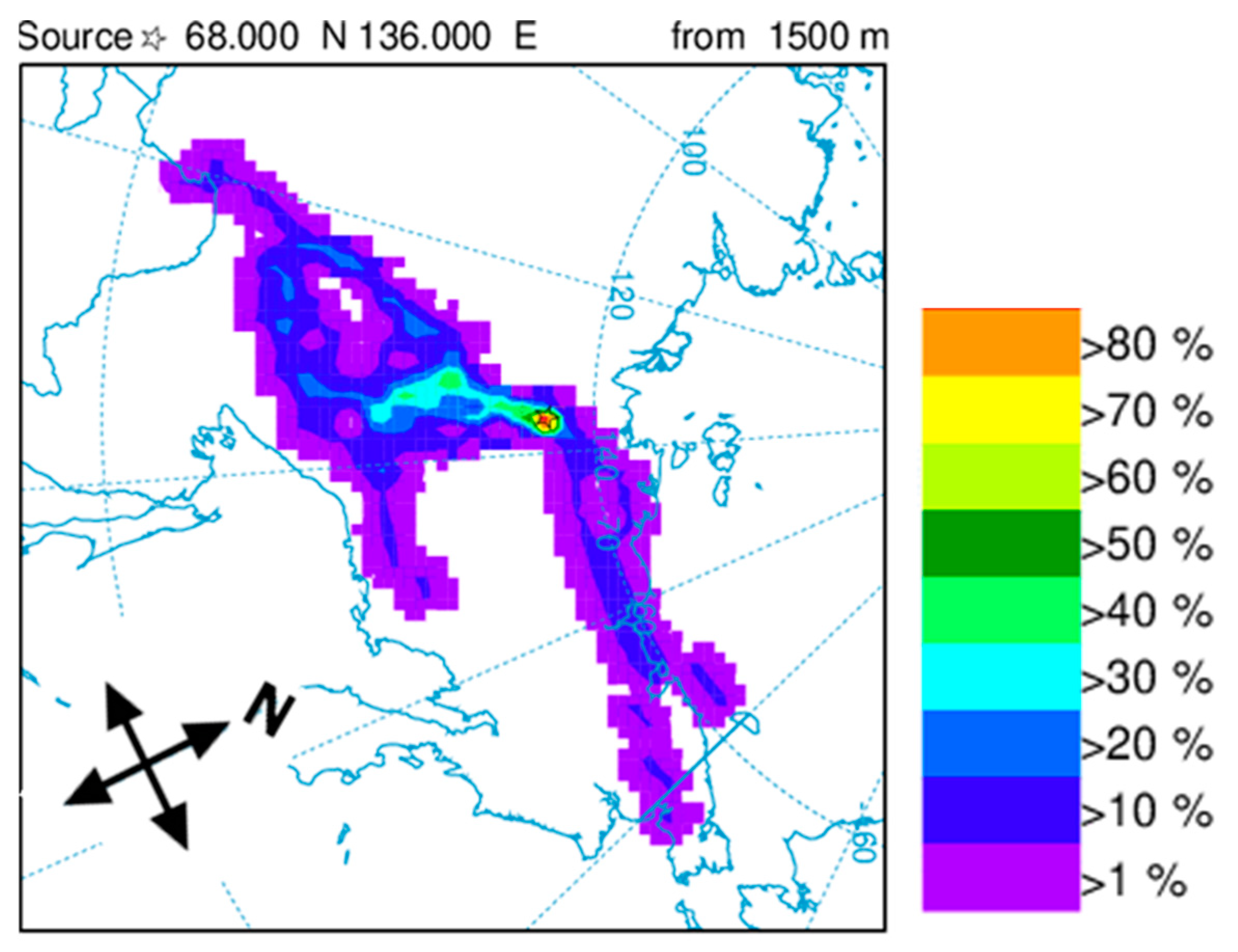
2.2. Description of the HYSPLIT Trajectory Model

The HYSPLIT trajectory model [25,26] was used to obtain a primary qualitative assessment of the possibility of particle transport from forest fires in Russia to an area covered with sea ice. This model is an autonomous system that allows calculation of the trajectories of both individual air particles and the entire complex of chemical transformation, dispersion and deposition of particles. The most common tasks for which the HYSPLIT model is applied is the calculation of back trajectories, as well as in modeling of the distribution of the pollutants, for example, smoke from forest fires, volcanic soot, and radioactive particles. The calculation method used in the model is a hybrid of the Lagrangian approach (for trajectory calculation) and the Euler method (for wind interpolation using a fixed three-dimensional grid). Several sources can be selected as the initial meteorological data, and we used the GDAS (The Global Data Assimilation System) reanalysis data. This is a system used in the National Center for Environmental Prediction (NCEP) global model for gridded observational data, including surface observations, wind profiler data, aircraft and radar observations, balloon data, satellite data and measurements from meteorological buoys.
The HYSPLIT model can compute the frequency with which the trajectory passes over a grid cell and then normalize by the total number of trajectories. A trajectory may intersect a 1° × 1° grid cell once or multiple times. The trajectory version of the HYSPLIT model, which calculates probabilities, permits running of the calculation for a maximum of 31 days. Therefore, for fires lasting more than 31 days, the calculation was still 31 days. For those fires lasting more than 6 days, the model was launched twice every day: at 00 UTC and 12 UTC. The computation time for each trajectory was 5 days—this is an estimate of the approximate lifetime of black carbon given in [7]. Thus, 62 trajectories were calculated for fires lasting a month or more. Then, the probability of occurrence of a particle carried from the fire zone to the Arctic zone was estimated. For short fires (lasting 1–6 days), the model was launched every 3 h: at 00, 03, 06, 09, 12, 15, 18, 21 UTC. The computation time for each trajectory was also 5 days. Thus, the number of trajectories for short fires involved in calculating of the probability ranged from 8 (for a one-day fire) to 48 (for a six-day fire). This was done to increase the number of trajectories so that the obtained probabilities were more comparable with the probabilities calculated for prolonged fires. The source height was set as equal to 1500 m.

3. Description of BC Emission Sources

Figure 1 shows the spatial distributions of BC sources corresponding to anthropogenic emissions for the period 1985–2014 [26], emissions due to burning biomass for the period 1985–2014 [27] and total emissions from forest fires in Siberia for 2019.
Black carbon emission from Siberian fires was calculated using the basic equation from IPCC Guidelines [28]:
Lfire = A × MB × Cf × Gef × 10−3
where:
  • Lfire—amount of BC emissions from fire, in tons;
  • A—total area burned, in ha
  • MB—mass of fuel available for combustion, in tons ha−1
  • Cf—combustion factor, dimensionless
  • Gef—emission factor, in g kg−1 dry matter burn.
Data on the area affected by wildfires, the area of fire disturbances on forested lands and on non-forested lands, both related to and not related to the forest fund, were taken from the national official forest authority—the Russian Federal agency for forestry (Rosleskhoz, Remote monitoring information system https://nffc.aviales.ru/main_pages/index.shtml accessed on 21 January 2020). The areas covered by fires of three types were identified: crown fire, surface fire and fires on lands not covered with forest vegetation (burned-out areas, clearings, dead stands) and on non-forest lands (glades, agricultural fields, etc.) [29]. The mass of fuel available for combustion was calculated by the ROBUL model [30,31] using State forest registry data. The combustion factor is 0.43 ± 0.21 for crown fire, 0.15 ± 0.08 for surface fire, 0.5 ± 0.25 for underground fire and 0.34 ± 0.17 for non-forest land fires (acc. table 2.6 27). Emission factor is 0.56 ± 0.19 for crown fires, ground fires and fires on non-forested lands, 0.20 ± 0.11 for underground fires and 0.91 ± 0.41 for non-forested lands [32]. The average uncertainty of estimations for black carbon emissions ranges from 69% to 74% for different types of fire. The total uncertainty for the federal districts decreases to 20–45%, and in the country as a whole in different years it is estimated at from 8% to 17% [33].
For the modelling experiment all forest fires in the Krasnoyarsk region and the Republic of Sakha (Yakutia) occurring in May–October 2019 were selected. The fires were ranked by classes depending on the intensity of black carbon emissions (up to 10 tons/day, from 10–20 tons/day, more than 20 tons/day). Based on fire duration and location, emission data were organized in the form of emission intensity (kg/s) for each cell of the model grid, separately for each intensity class for all days of the period.
It can be seen that the forest fire emission zone in Figure 1c is characterized by the absence of anthropogenic emissions. It can also be noted that emissions from forest fires in 2019 are comparable in value to the average climate component of emissions from forest fires for the period 1985–2014, prepared within the framework of the CMIP6 project.
Figure 2 shows the time course of total emissions from forest fires in Siberia in 2019 for three different types of fire, mainly differing in the height of emissions: the first class: smoldering ground fires, usually long-term—emission height no more than 100 m; the second class: mixed ground and top fires—discharge height 500 m; the third class: powerful top fires with high discharge into the atmosphere—discharge height 1500 m.
Emission sources corresponding to the different classes were set at model levels, the height of which approximately corresponded to the above values (100 m, 500 m, 1500 m). Table 1 presents a total emission intensity averaged for the Arctic region and global average values. It is noticeable that emissions from forest fires in Siberia are only about two times less than the average annual anthropogenic emissions for the Arctic.
Table 2 shows data for the most severe fires during the Summer of 2019, prepared by the IGCE. All these fires were located in Siberia, most of them in the Sakha (Yakutia) Republic and the Krasnoyarsk Territory. The probabilities of particle transport to the Arctic for these fires were calculated using the Hysplit trajectory model. In contrast to the experiments with the climate model, where emissions were set at three different levels, in the experiments with Hysplit we set the height of the emission at 1500 m, which corresponds to class 3—powerful crown fires with intensive throwing into the atmosphere.

4. Numerical Experiments

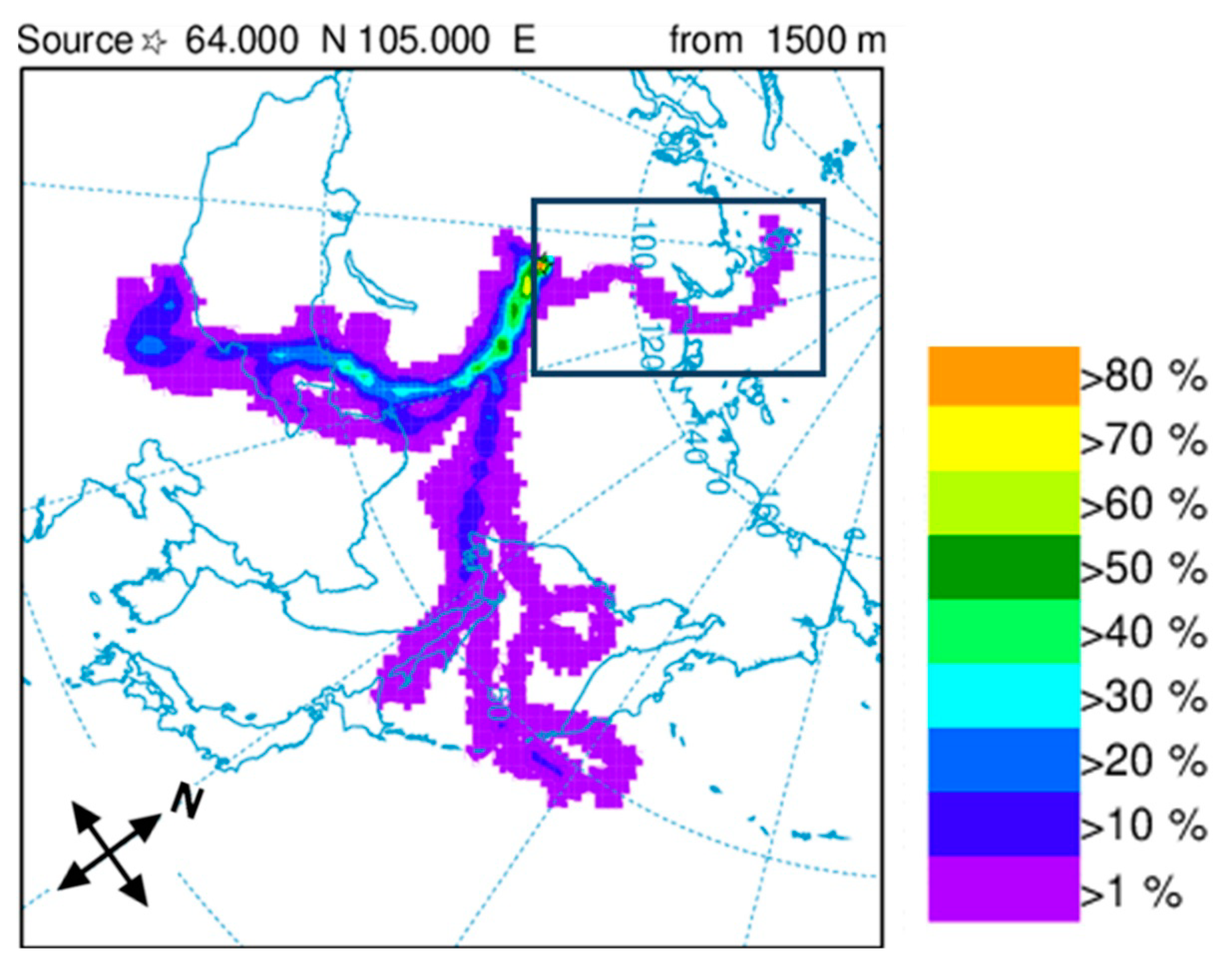
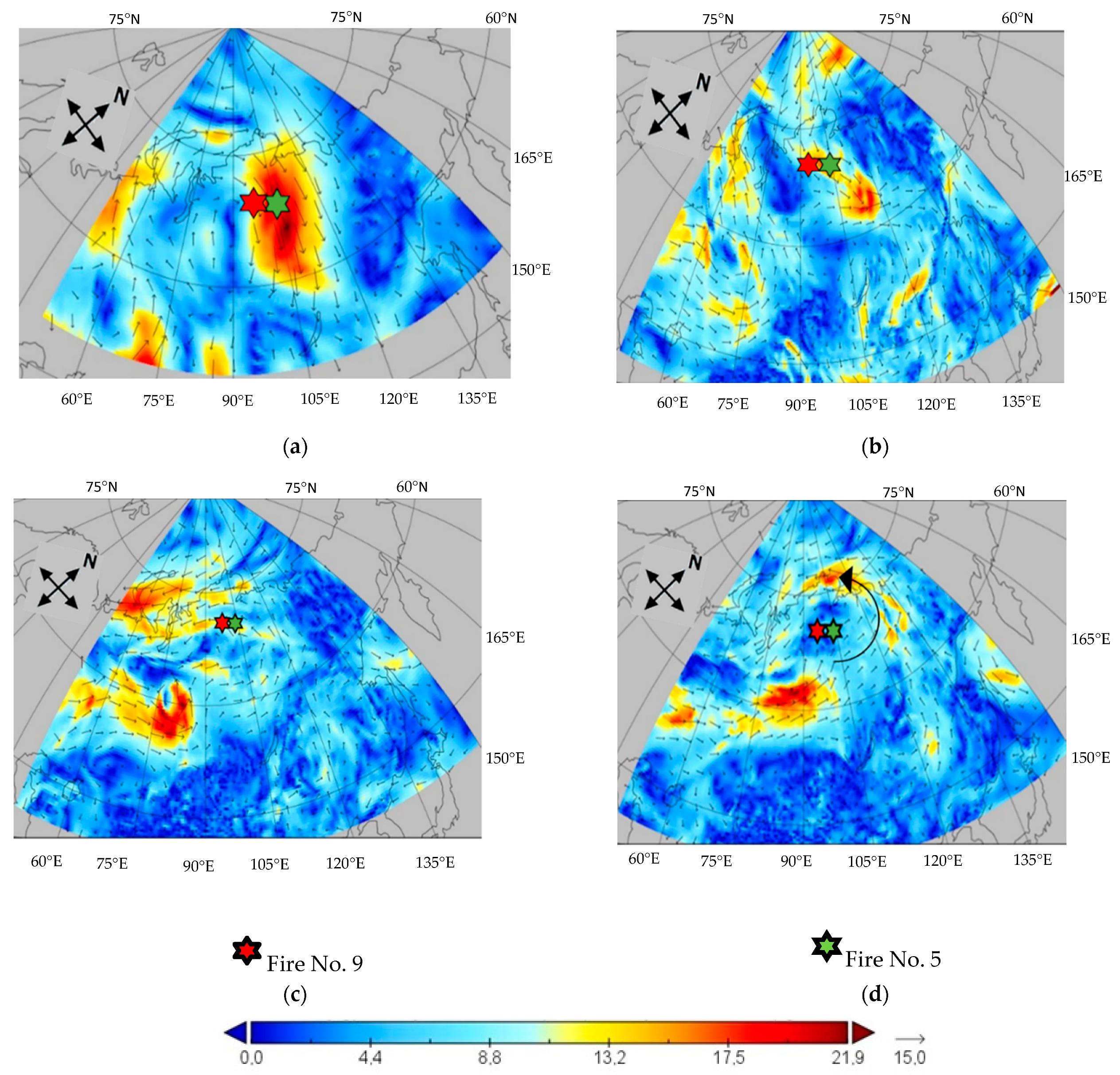
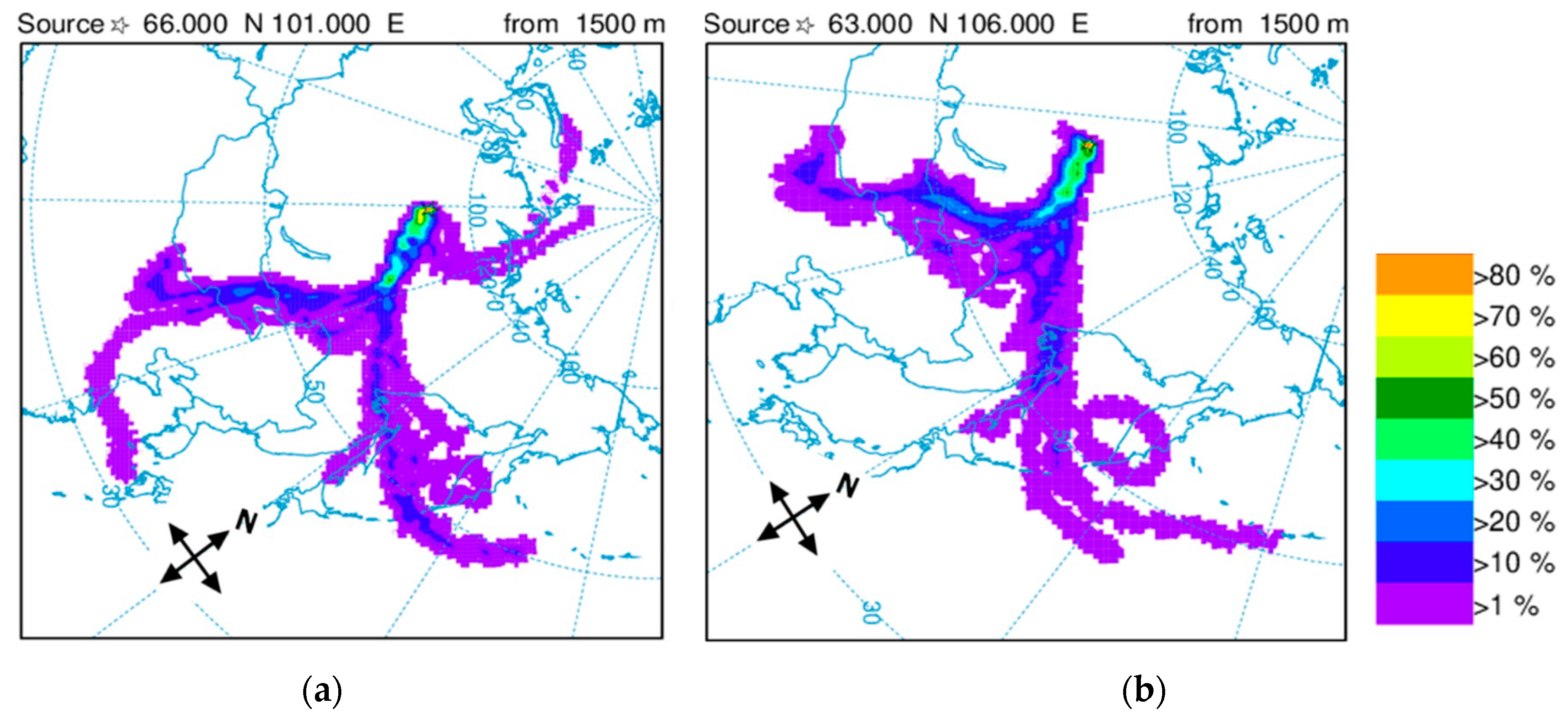
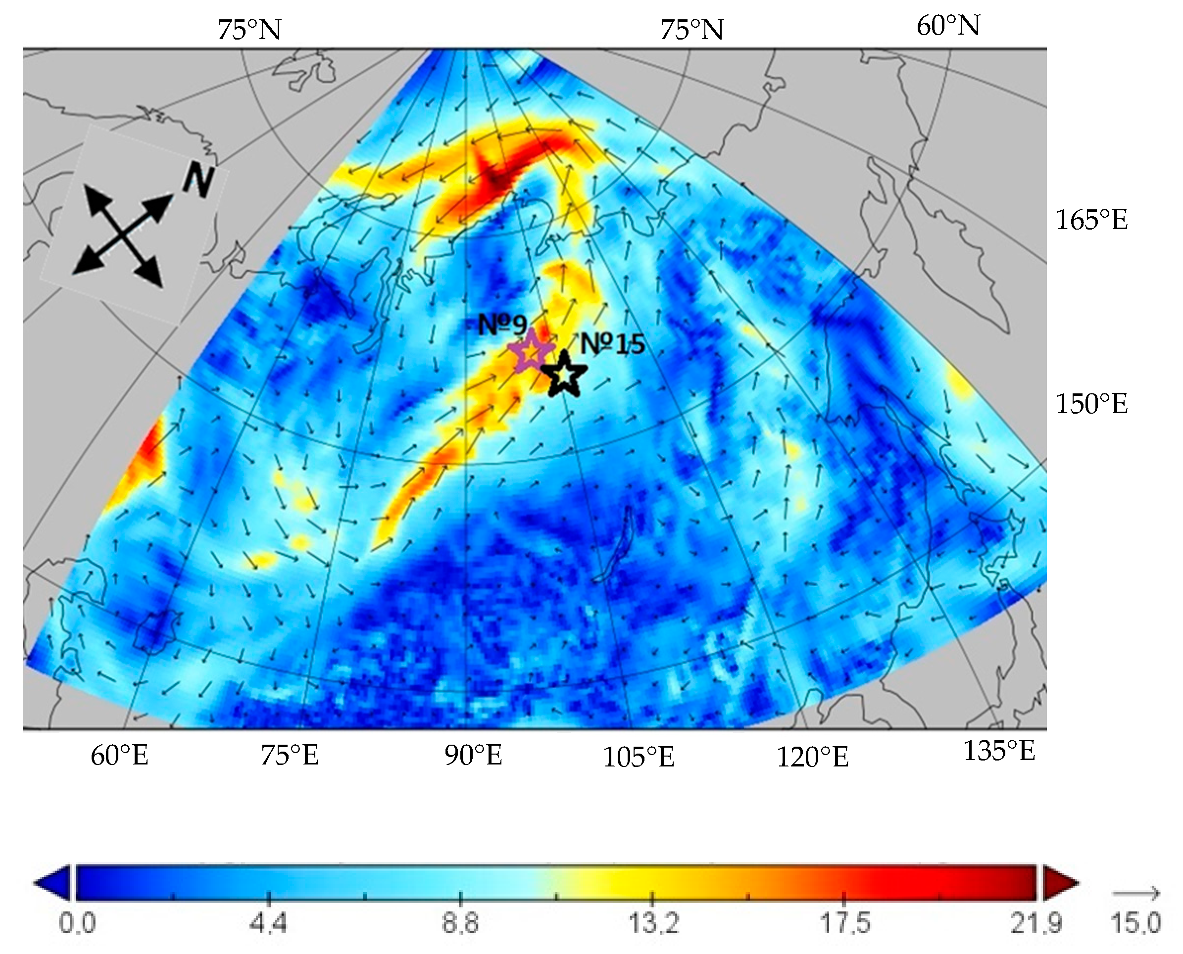
4.1. Numerical Experiments with the HYSPLIT Model

Experiments with the HYSPLIT trajectory model can only give us a qualitative assessment of the possibility of transfer of the particles from fires to the Arctic zone. Nevertheless, we believe that an analysis of individual fire events and synoptic conditions during this period will help to understand the mechanism of transport of particles from the source. We used the Hysplit model to calculate the trajectory frequency. The model starts a trajectory from a single location and height, sums the frequency that the trajectory passes over a grid cell and then normalizes by either the total number of trajectories or endpoints. It is important to notice that a trajectory may intersect a grid cell once or multiple times. With this in mind, we will further operate on the concept of probability of particle transfer maps”. As mentioned above, all the fires considered took place in Siberia (mainly in the Krasnoyarsk Territory and in Yakutia). During long-term fires (lasting a month or more), the distribution pattern of the probability of a particle passing a particular cell is comparable: the highest probability is in cells located near the source. The transfer probability decreases up to 1%–10% with an increase in the distance from the fire, while only single trajectories reach the cells in the Arctic (Figure 3). Some even reach North America (Figure 3a,b), and others end in the East Siberian, Kara and Laptev Seas.
The probability of particle transport from fires lasting 1–2 days is significantly more dependent on the synoptic situation and on the day of the fire (Figure 4, Figure 5, Figure 6, Figure 7 and Figure 8). For example, fire No. 5, which appeared in the east of the Krasnoyarsk Territory in the Taimyr peninsula, occurred during a synoptic situation contributing to the transfer of particles to the south—to the Trans-Baikal Territory and Mongolia; thus, from 30% to 40% of the trajectories were directed there. From 10% to 20% of the trajectories had an eastern direction, and from 1% to 10% reached the Arctic. The calculated trajectories were calculated for 5 days and started every 3 h.
Wind maps on an isobaric surface of 850 hPa (which roughly corresponds to 1500 m, the height of the ejection specified in the model) are presented in Figure 5. These maps were obtained from the ERA5 reanalysis for several days, starting from 3 July 2019 (the initial day of the fire). It can be seen that a stable north wind prevailed with speeds of 25 m/s or more on the first day of ignition, at an altitude of 850 hPa (Figure 5a). On the next day, 4 July, the wind changed direction to the west (Figure 5b), supporting the transfer of particles to the East. A rather weak wind of variable directions was observed in the next two days—5–6 July. On 7 July, the wind changed direction to the south (Figure 5c). The wind increased on 8 July. It can be seen that the leading stream, passing through the northwest of the Sakha (Yakutia) Republic, bends around Taimyr (Figure 5d). The same trajectory is visible on the map of the distribution of the probability of particle transport (Figure 4).
Fire No. 9 also occurred on 3 July and lasted for only 2 days, appearing a little further to the west than fire No. 5. In general, the map of the probability distribution of particles transfer from fire No. 9 (Figure 6a) is similar to the distribution map of trajectories during fire No. 5 (Figure 4): three transport directions prevail: southern, eastern and northern, but in this case approximately equal numbers of particles are transported to the south and east, which is apparently associated with weaker speeds of the north wind on the first day at the source of the fire (Figure 5a).
It is noteworthy that the map of particle transport from fire no. 15 (Figure 6b) differs from the previous two, despite the fact that this fire also occurred on 3 July. The absence of a transport trajectory directed to the Arctic is probably due to the more southeastern location of the ignition source (near the border of the Krasnoyarsk Territory with the Irkutsk Region), and as a result the particles did not enter the “jet” directed to the north.
Fire No. 16 appeared on June 28 in the north of the Sakha (Yakutia) Republic near the Verkhoyansk at a relatively short distance from the Arctic coast. It lasted for only one day and a significant number of particle transfer trajectories on this day and the next 5 days were directed south (from 30% to 40%). From 1% to 20% of the transfer trajectories fell into the East Siberian Sea (Figure 8). This is a rather rare case, showing that, even with a short but powerful fire, up to 20% of particles can be transported to the Arctic under favorable synoptic conditions and the location of the ignition source is a relatively short distance from the coast.

4.2. Numerical Experiments with INMCM5model

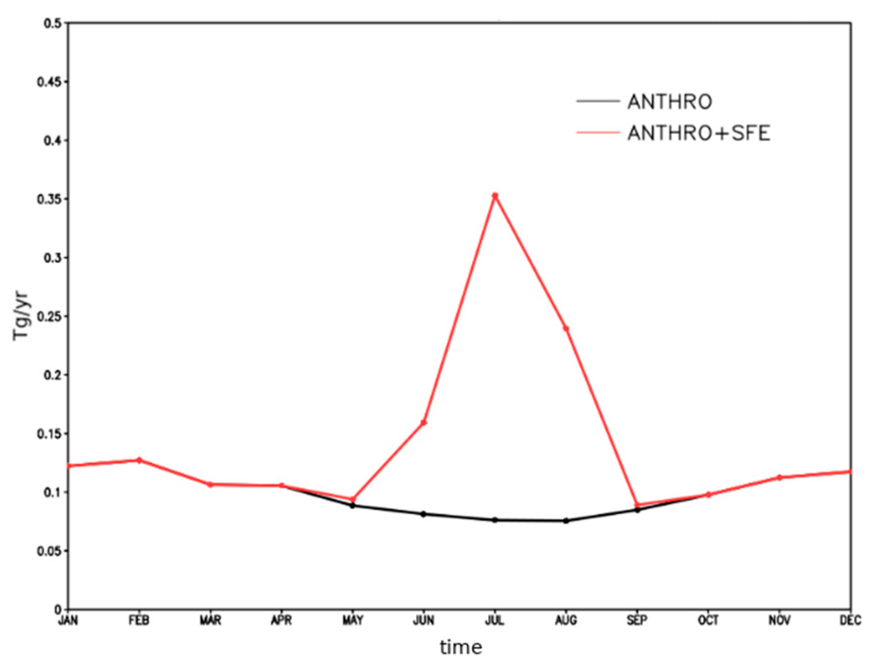
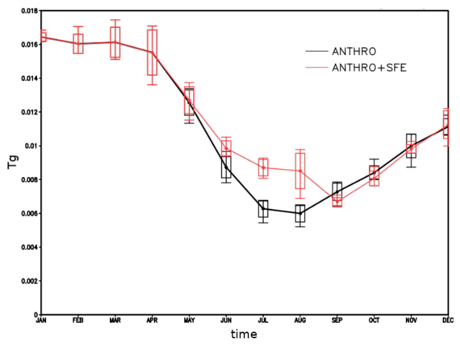
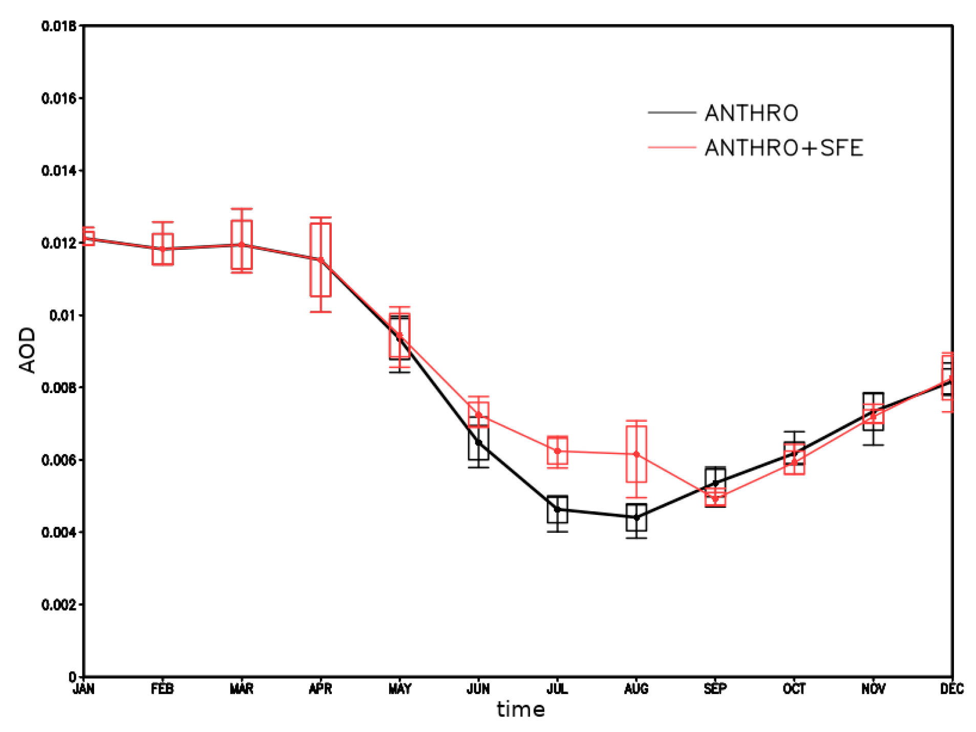
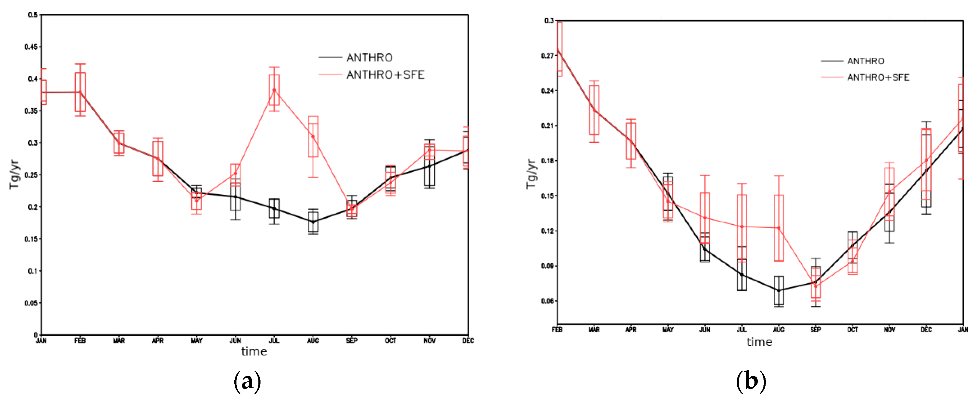
4.2.1. Emissions and Atmospheric Effects

The seasonal cycle of BC emission in the Arctic (60–90° N) is presented in Figure 9. It increases by 3–4 times in the summer months due to the Siberian fires. The peak of additional emissions from fires is in July.
The total BC burden in the atmosphere over the Arctic zone during the year is depicted in Figure 10. It can be noted that the total BC burden in the Arctic atmosphere increases on average by 50% in July and August. This contribution is made by emissions from fires shown in Figure 9. It is noteworthy that the total content of BC (Figure 9) increases in the summer months is not in direct proportion to the increase in BC emission during this period (Figure 2). This is due to the fact that some of the particles are transported to the south and carried out from the Arctic zone. This mechanism was discussed in more detail in Section 4.1 where data from the Hysplit model are presented.
The seasonal variation of the average optical depth in the Arctic can be seen in Figure 11. It can be seen that, on average, the optical thickness of the atmosphere over the Arctic increases by 0.0015 in July and August. If we assume that the flux of incoming solar radiation at this time is about 250 W/m2, then for the Arctic as a whole we will obtain an estimate of the effect of attenuation of the incoming solar radiation due to atmospheric BC in July–August by 0.3–0.4 W/m2.

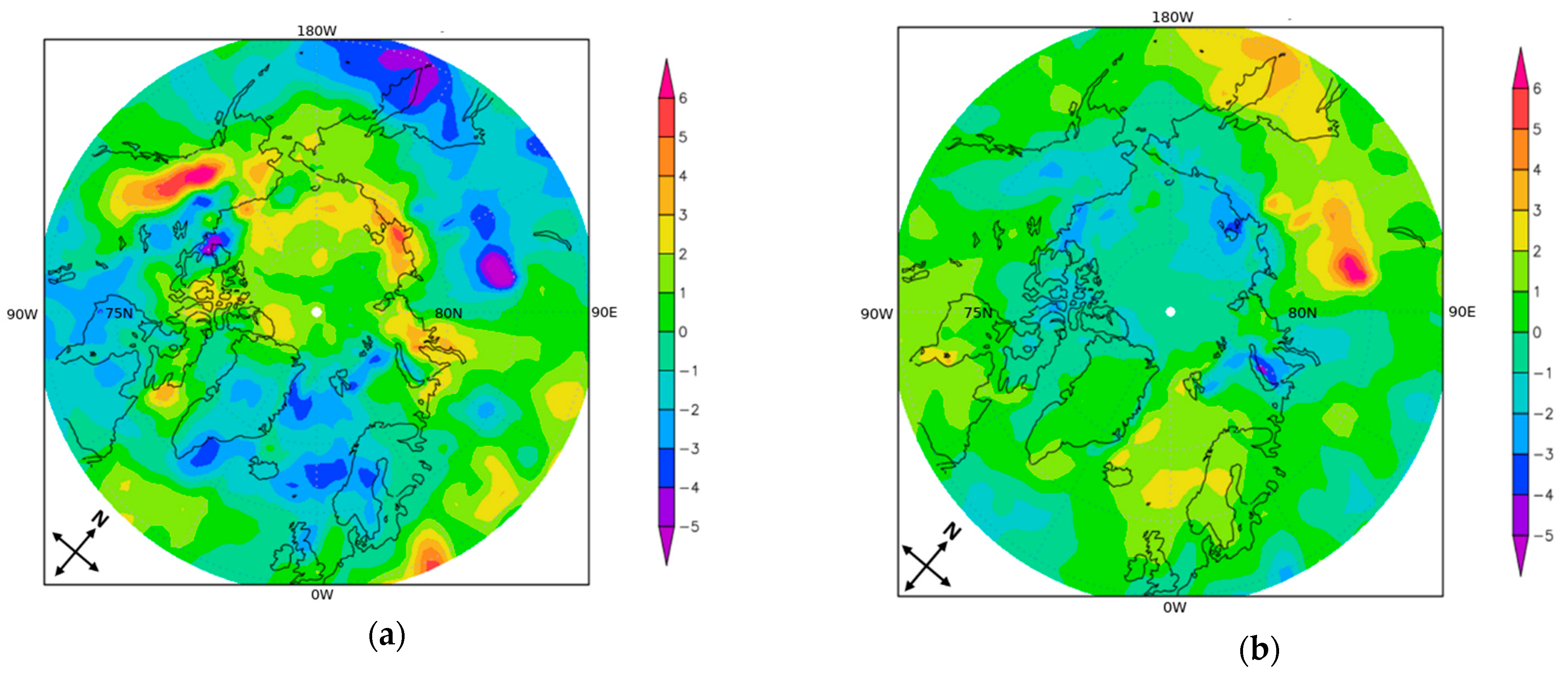
4.2.2. Changes in the Main Radiation Parameters

The maps of the ensemble-averaged BC optical thickness anomaly in July and August are presented in Figure 12. It can be noticed that the maximum of the BC optical thickness anomaly is located over the territory of Siberia (mainly over Yakutia and the Krasnoyarsk Territory) in the zone of localization of the strongest fires and can reach 0.03 in July and 0.015 in August.
Maps of the ensemble-averaged anomaly of incoming solar radiation on the surface and radiation heating of the atmosphere, with a clear sky in July, are shown at Figure 13. The influence of BC emissions in the zone of the main fires is evidently traced in these maps. It follows from Figure 13a that the weakening of the solar radiation flux due to atmospheric BC can reach 4–5 W/m2. The location of the Siberian minimum of the solar radiation inflow anomaly coincides approximately with the location of the maximum atmospheric radiation heating anomaly. The amount of heat inflow into the atmosphere also roughly corresponds to the amount of attenuation of the solar radiation flux on the surface and is at a maximum of 5–6 W/m2 (Figure 13b).

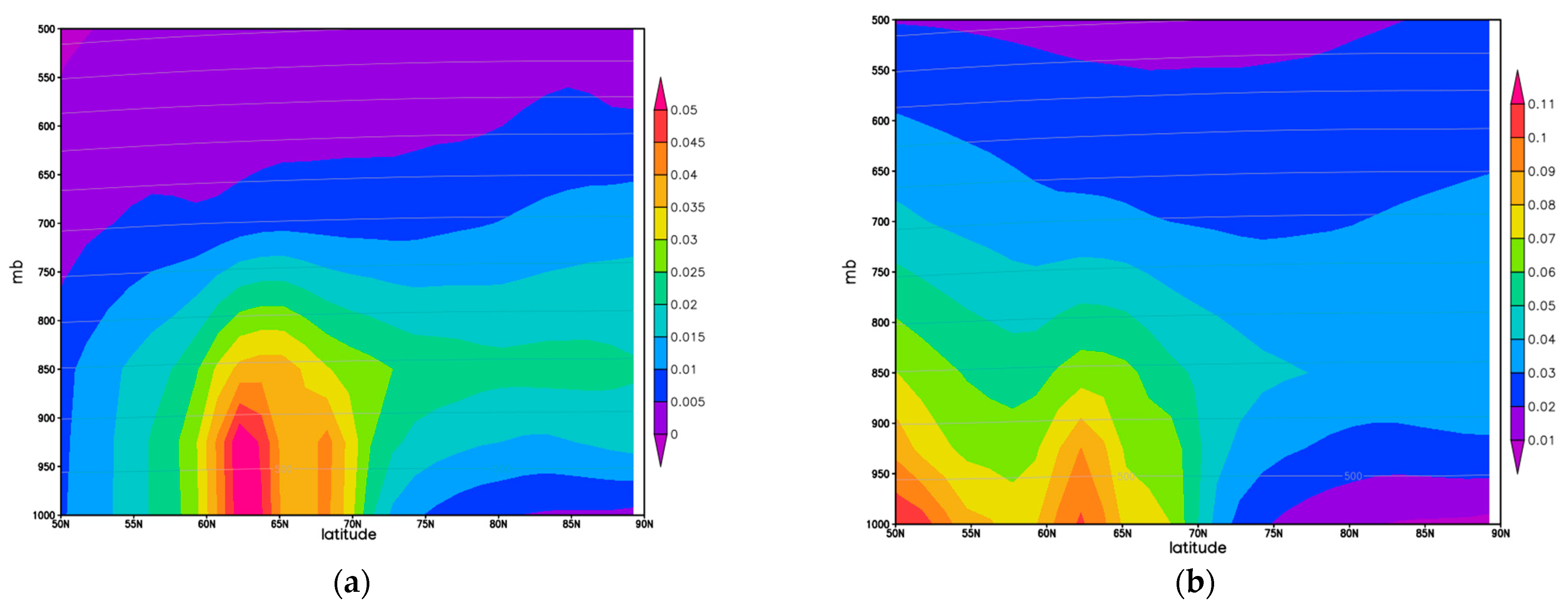
4.2.3. Vertical Profiles of Black Carbon

The vertical profiles of the zonal mean anomaly of the BC concentration and the total BC concentration in the ANTHRO+SFE experiment in August is depicted in Figure 14. It can be seen that the maximum BC concentration anomaly is located near the surface (1000–900 hPa) in the latitudinal zone from 60 to 65 N with a gradual decrease to 70 N. In general, this corresponds to the location of the main fires (see Table 2) and indicates that most of the BC is not transported over considerable distances from the source. Figure 14a shows that the maximum of the zonal mean BC concentration over the Arctic territory to the north of the emission zone in August is located at an altitude of 1.5 km (850 hPa). Similar results are presented in [14], showing that the transport of black carbon to the Arctic occurs above the atmosphere boundary layer at altitudes from 2 to 6 km, where aerosol particles have a longer lifetime due to less intensive removal from the atmosphere. The height of BC transport routes corresponds to the height of emissions from the most powerful fires, specified both in experiments with the INMCM model and in experiments with the Hysplit model. At lower altitudes (below 1.5 km), the BC concentration decreases, most likely due to the wet and dry deposition.
The maximum monthly average anomaly of BC concentration in the atmosphere reaches 0.05 μg/m3 above the emission zone and is approximately two times less outside the emission zone. From Figure 14b, it also follows that the anomaly of the BC concentration in the atmosphere is quite significant compared to the background BC concentration.

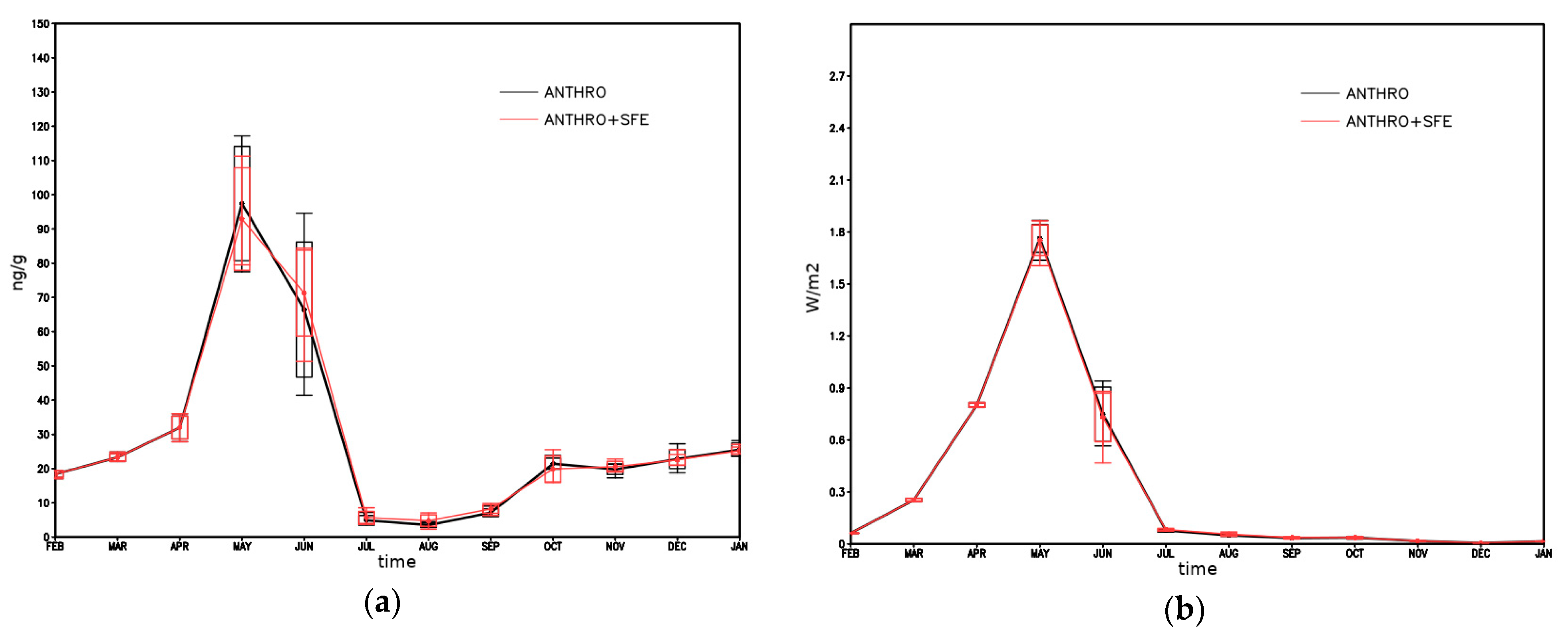
4.2.4. Effects Associated with the Deposition of BC on the Surface

The annual course of BC deposition on the surface in the Arctic (north of 60 N) and on sea ice in the Arctic can be seen in Figure 15.
BC deposition in the Arctic increases by about 1.5–2 times in July and August when accounting for emissions from forest fires (Figure 15). The maximum deposition of BC on the surface in the Arctic occurs in July and coincides with the period of maximum emission. Note that the maximum BC deposition on the sea ice surface has shifted to August. This delay is caused by the time of transfer of BC particles from the emission zone located beyond the polar circle. According to model estimates, the characteristic lifetime of BC aerosol particles in the Arctic atmosphere north of 70 N is 20 days in the summer months.
The seasonal variation of the average BC concentration in the snow and the corresponding radiation forcing in the Arctic is depicted in Figure 16. It should be noted that snow cover in July and August is very thin or absent for many locations in the Arctic.
Calculation of BC influence on ice albedo needs a completely different approach comparing to those we used for modelling BC concentration in snow and its albedo effect. In this study we have investigated only the effects associated with the deposition of BC on snow surfaces with a layer >1 mm. This assumption leads to underestimation of BC concentration and corresponding radiation forcing in July and August. As a result, maximum concentration of BC in snow as well as radiation forcing is obtained in May and reaches values of 100 ng/g and 1.8 W/m2. The average concentration of BC is 2.7 ng/g in snow on sea ice in the ANTRO experiment in August, and equal to 3.9 ng/g in the ANTHRO + SFE experiment. Thus, the average concentration of BC in snow on sea ice is increases by 45% in this month. Similarly, the mean radiative forcing for BC in snow on sea ice increases by 45%, from 0.016 W/m2 to 0.023 W/m2. However, over the year the radiation forcing is minimal in the winter season, which is associated with the absence of insolation at high latitudes at this time. Since the main changes in BC concentration in snow associated with fires occur in July–August, when the BC concentration in snow is minimal and the radiation forcing is rather small, it can be argued that the impact from forest fires will be insignificant on average for the year.
However, locally the anomalies of the considered values can be quite significant. The field anomaly of BC concentration in snow on sea ice in August and the anomaly of radiation forcing for one realization, which turned out to be maximum, are presented in Figure 17. We see that local anomalies in the concentration (radiation forcing) of BC in snow can reach 100–150 ng/g (0.5–1 W/m2).

5. Discussion

Black carbon emissions undoubtedly affect the Arctic climate [1,14,16,17,18,34,35]. However, which sources make the greatest contribution to the formation of BC concentration in the Arctic region and what are the mechanisms for BC influence on the Arctic climate are still under discussion. A number of studies show that black carbon emissions from forest fires in Russia are one of the main sources of black carbon in the Arctic region and, as a result, one of the main reasons for the increase in melting ice in the Arctic. Unfortunately, official information on forest fires in Russia is very limited and the scatter of the associated emission estimates is very large. We estimate the average uncertainty of estimations for black carbon emissions ranges from 69% to 74% for different types of fire. In our work, we focused on the impact of forest fires that occurred in the summer of 2019 in Russia on the Arctic climate. Our estimates are based on the data for forest fires provided by the national official forest authority—the Russian Federal agency for forestry— and divided fires by types with different emission parameters. We believe that total uncertainty for the federal districts decreases to 20–45%, and in the country as a whole in different years this is estimated at 8% to 17%. However, the refinement of the calculated parameters and the initial data for estimating emissions from forest fires should be carried out further in order to obtain more realistic estimates.
The results obtained using the HYSPLIT model helped us to understand what percentage of trajectories from the fire zone were actually directed to the Arctic. The direction of transfer depends on the synoptic situation, but for prolonged fires (lasting more than 10 days) there is practically no dependence on the synoptic situation. About 1% to 10 percent of the trajectories can reach the Arctic, and theoretically transfer black carbon emitted as a result of strong fires.
We have attempted to estimate the radiative effect of BC in the Arctic both in the atmosphere due to its dimming and at the surface due to snow darkening by BC from the additional source of Siberian forest fires in 2019, using the INMCM5 climate model. Experiments with different sources of black carbon (with and without forest fire emissions) have shown that the radiative effect is sufficiently small if one considers the average effect on the Arctic, but could be much stronger locally. Generally, the effect of black carbon on the radiation balance is found in an increase in the optical thickness and, as a consequence, in a decrease in the flux of direct solar radiation entering the underlying surface; in radiative heating of the atmosphere as a result of thermal radiation from black carbon particles; and in an increase in BC concentration in the atmosphere and deposition fluxes on the underlying surface.
Simulation of BC–snow and BC–ice interaction and BC influence on albedo is a very complex task. In this study we have investigated only effects associated with the deposition of BC on snow surface with a layer >1 mm, because calculation of BC influence on ice albedo needs a completely different approach. This could lead to underestimation of radiative effects from BC on surface albedo, especially as in summer snow cover is very thin or absent from many locations in the Arctic. However, we still found a quite significant local influence of BC on the surface albedo in August for regions with existing snow on ice.
The results of the study may be useful for comparison with other climate model studies using BC emissions from extremely strong forest fires in Siberia estimated from different inventories in experiments with an INMCM climate model. Our research shows a need for more refined estimates of black carbon emissions and investigation of the mechanisms of its interaction with the underlying surface, in particular in the absence of snow cover on ice.

6. Conclusions

Two tools were used to assess the possible impact of BC emissions from wildfires on the Arctic zone. The HYSPLIT trajectory model was used for the initial qualitative assessment of the possibility of particle transport from Siberian fires. The results show that the probability of the transfer of particles to the Arctic ranges from 1% to 10%, and rises to 20% in some cases. The dependence on the synoptic situation is significantly greater in the case of short-term fires than in the case of prolonged ones. More detailed studies of the possible influence of BC ejected as a result of fires were carried out using the INMCM climate model. It was possible to estimate, following the effects of BC, changes in the radiation balance, in snow surface albedo, and in radiation forcing. These experiments simulate the response to the Siberian forest fires in 2019 and have shown that the maximum concentration of BC in the Arctic atmosphere is observed in July–August and increases in these months by 3.5 times, precisely due to the fire component. The total BC content in the Arctic atmosphere increases by 50% on average in July and August. It does not increase in direct proportion to the BC emission increase during this period, which is apparently associated with the partial removal of particles from the Arctic zone. Direct radiative forcing from BC in the atmosphere with a clear sky is at a maximum of 4–5 W/m2 in July–August. The absorbed short-wave radiation is used to heat the atmospheric column. The maximum concentration of BC outside the emission zone over the Arctic is observed at an altitude of 1.5 km. The maximum precipitation anomaly in BC due to forest fires is observed in July–August. At the same time, the average concentration of BC in snow on sea ice in the Arctic and the corresponding radiation forcing can increase by 45%. Typical values of average anomalies of BC concentration in snow on sea ice are 1 ng/g, and radiation forcing is 0.01 W/m2. Local anomaly of radiation forcing from snow coverage of BC in August can be at a maximum 1 W/m2, and local anomaly of BC concentration in snow at 100–150 ng/g.

Author Contributions

Conceptualization, S.K. and V.G.; methodology, S.K. and V.G.; software, A.C. and A.R.; validation, S.K., A.R. and V.G.; formal analysis, S.K.; investigation, P.P., A.C. and M.Z.; resources, S.K. and V.G.; data curation, M.Z., P.P.; writing—original draft preparation, S.K., A.R. and V.G.; writing—review and editing, A.R.; visualization, S.K. and A.R.; supervision, V.G.; project administration, M.Z.; funding acquisition, M.Z. All authors have read and agreed to the published version of the manuscript.

Funding

The study was co-funded by the Russian Foundation for Basic Research, grant No 18-05-60183 (research design, preparation of forest fire emission data, numerical experiments with HYSPLIT model, article preparation and publication fee) and the Russian Science Foundation, grant No 20-17-00190 (numerical experiments with climate model performed at the Marchuk Institute of Numerical Mathematics of the Russian Academy of Sciences).

Institutional Review Board Statement

Not applicable.

Informed Consent Statement

Informed consent was obtained from all subjects involved in the study.

Data Availability Statement

Publicly available resources were used in this study. Them can be found here: https://www.ready.noaa.gov/HYSPLIT.php (accessed on 12 February 2020). Restrictions apply to the availability of the data retrieved from INMCM model simulations.

Acknowledgments

The authors gratefully acknowledge the NOAA Air Resources Laboratory (ARL) for the provision of the HYSPLIT transport and dispersion model and/or READY website (https://www.ready.noaa.gov accessed on 21 January 2020) used in this publication. We also thank two reviewers for valuable comments to improve our article.

Conflicts of Interest

The authors declare no conflict of interest.

References

  1. Bond, T.C.; Doherty, S.J.; Fahey, D.W.; Forster, P.; Berntsen, T.; DeAngelo, B.J.; Flanner, M.G.; Ghan, S.; Kaercher, B.; Koch, D.; et al. Bounding the role of black carbon in the climate system: A scientific assessment. J. Geophys. Res. Atmos. 2013, 118, 5380–5552. [Google Scholar] [CrossRef]
  2. Lavoué, D.; Liousse, C.; Cachier, H.; Stocks, B.J.; Goldammer, J.G. Modeling of carbonaceous particles emitted by boreal and temperate wildfires at northern latitudes. J. Geophys. Res. Space Phys. 2000, 105, 26871–26890. [Google Scholar] [CrossRef] [Green Version]
  3. IPCC. Climate Change 2013: The Physical Science Basis. Contribution of Working Group I to the Fifth Assessment Report of the Intergovernmental Panel on Climate Change; Stocker, T.F., Qin, D., Plattner, G.-K., Tignor, M., Allen, S.K., Boschung, J., Nauels, A., Xia, Y., Bex, V., Midgley, P.M., Eds.; Cambridge University Press: Cambridge, UK; New York, NY, USA, 2013; 1535p. [Google Scholar]
  4. AMAP. Arctic Monitoring and Assessment Programme, Assessment 2015: Black Carbon and Ozone as Arctic Climate Forcers; AMAP: Oslo, Norway, 2015; p. vii. 116p, ISBN 978-82-7971-092-9. [Google Scholar]
  5. Shindell, D.; Faluvegi, G. Climate response to regional radiative forcing during the twentieth century. Nat. Geosci. 2009, 2, 294–300. [Google Scholar] [CrossRef]
  6. UNEP; WMO. Integrated Assessment of Black Carbon and Tropospheric Ozone; UNON/Publishing Services Section: Nairobi, Kenya, 2011. [Google Scholar]
  7. Koch, D.; Schulz, M.; Kinne, S.; McNaughton, C.; Spackman, J.R.; Balkanski, Y.; Bauer, S.; Berntsen, T.; Bond, T.C.; Boucher, O.; et al. Evaluation of black carbon estimations in global aerosol models. Atmos. Chem. Phys. Discuss. 2009, 9, 9001–9026. [Google Scholar] [CrossRef] [Green Version]
  8. Karol, I.L.; Kiselev, A.A.; Genikhovich, E.L.; Chicherin, S.S. Reducing Emissions of Short-Lived Atmospheric Pollutants as an Alternative Strategy for Slowing Climate Change; Izv. RAS Series; FAO: Roma, Italy, 2013; Volume 49, pp. 503–522. [Google Scholar]
  9. Huang, K.; Fu, J.S.; Prikhodko, V.Y.; Storey, J.M.; Romanov, A.; Hodson, E.L.; Cresko, J.; Morozova, I.; Ignatieva, Y.; Cabaniss, J. Russian anthropogenic black carbon: Emission reconstruction and Arctic black carbon simulation. J. Geophys. Res. Atmos. 2015, 120, 11306–11333. [Google Scholar] [CrossRef]
  10. U.S. EPA. Report to Congress on Black Carbon; US Environmental Protection Agency: Washington, DC, USA, 2012. Available online: http://www.epa.gov/blackcarbon/ (accessed on 26 November 2019).
  11. Romanovskaya, A.A.; Imshennik, E.V.; Karaban, R.T.; Smirnov, N.S.; Korotkov, V.N.; Trunov, A.A. Emissions of short-lived climatically active pollutants of anthropogenic origin on the territory of Russia for the period from 2000 to 2013. Probl. Environ. Monit. Ecosyst. Model. 2016, XXVII. [Google Scholar] [CrossRef]
  12. Vinogradova, A.A.; Smirnov, N.S.; Korotkov, V.N. Anomalous fires in 2010 and 2012. on the territory of Russia and the flow of black carbon into the Arctic. Opt. Atmos. Ocean 2016, 29, 482–487. [Google Scholar] [CrossRef]
  13. Vinogradova, A.A.; Smirnov, N.S.; Korotkov, V.N.; Romanovskaya, A.A. Forest fires in Siberia and the Far East: Emissions and atmospheric transport of black carbon to the Arctic. Opt. Atmos. Ocean 2015, 28, 512–520. [Google Scholar] [CrossRef]
  14. Ginzburg, V.A.; Kostrykin, S.V.; Revokatova, A.P.; Ryaboshapko, A.G.; Pastukhova, A.S.; Korotkov, V.N.; Polumieva, P.D. Short-lived climate-forming aerosols from forests fires ith territory of Russia: Model estimates of the probability of the transfer to the Arctic and possible effect on the regional climate. Fundam. Appl. Climatol. 2020, 1, 21–41. [Google Scholar] [CrossRef]
  15. Srivastava, R.; Ravichandran, M. Spatial and seasonal variations of black carbon over the Arctic in a regional climate model. Polar Sci. 2021, 100670. [Google Scholar] [CrossRef]
  16. Flanner, M.G. Arctic climate sensitivity to local black carbon. J. Geophys. Res. Atmos. 2013, 118, 1840–1851. [Google Scholar] [CrossRef]
  17. Sand, M.; Berntsen, T.K.; Kay, J.E.; Lamarque, J.F.; Seland, Ø.; Kirkevåg, A. The Arctic response to remote and local forcing of black carbon. Atmos. Chem. Phys. 2013, 13, 211–224. [Google Scholar] [CrossRef] [Green Version]
  18. James, H.; Larissa, N. Soot climate forcing via snow and ice albedos. Proc. Natl. Acad. Sci. USA 2004, 101, 423–428. [Google Scholar]
  19. Volodin, E.M.; Mortikov, E.V.; Kostrykin, S.V.; Galin, V.Y.; Lykossov, V.N.; Gritsun, A.S.; Diansky, N.A.; Gusev, A.V.; Iakovlev, N. Simulation of the present-day climate with the climate model INMCM5. Clim. Dyn. 2017, 49, 3715–3734. [Google Scholar] [CrossRef]
  20. Volodin, E.M.; Mortikov, E.V.; Kostrykin, S.V.; Galin, V.Y.; Lykossov, V.N.; Gritsun, A.S.; Diansky, N.A.; Gusev, A.V.; Iakovlev, N.G.; Shestakova, A.A.; et al. Simulation of the modern climate using the INM-CM48 climate model. Russ. J. Numer. Anal. Math. Model. 2018, 33, 367–374. [Google Scholar] [CrossRef]
  21. Flanner, M.G.; Zender, C.S.; Randerson, J.T.; Rasch, P.J. Present-day climate forcing and response from black carbon in snow. J. Geophys. Res. 2007, 112, D11202. [Google Scholar] [CrossRef] [Green Version]
  22. Volodin, E.M.; Kostrykin, S.V.; Ryaboshapko, A.G. Climate response to aerosol injection at different stratospheric locations. Atmos. Sci. Lett. 2011, 12, 381–385. [Google Scholar] [CrossRef]
  23. Volodin, E.M.; Kostrykin, S.V. The Aerosol module in the INM RAS climate model. Rus. Meteorol. Hydrol. 2016, 41, 519–528. [Google Scholar] [CrossRef]
  24. Chernenkov, A.Y.; Kostrykin, S.V. Estimation of Radiative Forcing from Snow Darkening with Black Carbon Using Climate Model Data. Izv. Atmos. Ocean. Phys. 2021, 57, 133–141. [Google Scholar] [CrossRef]
  25. Stein, A.F.; Draxler, R.R.; Rolph, G.D.; Stunder, B.J.B.; Cohen, M.D.; Ngan, F. NOAA’s HYSPLIT Atmospheric Transport and Dispersion Modeling System. Bull. Am. Meteorol. Soc. 2015, 96, 2059–2077. [Google Scholar] [CrossRef]
  26. Rolph, G.; Stein, A.; Stunder, B. Real-time Environmental Applications and Display sYstem: READY. Environ. Model. Softw. 2017, 95, 210–228. [Google Scholar] [CrossRef]
  27. Hoesly, R.M.; Smith, S.J.; Feng, L.; Klimont, Z.; Janssens-Maenhout, G.; Pitkanen, T.; Seibert, J.J.; Vu, L.; Andres, R.J.; Bolt, R.M.; et al. Historical (1750–2014) anthropogenic emissions of reactive gases and aerosols from the Community Emissions Data System (CEDS). Geosci. Model Dev. 2018, 11, 369–408. [Google Scholar] [CrossRef] [Green Version]
  28. Van Marle, M.J.E.; Kloster, S.; Magi, B.I.; Marlon, J.R.; Daniau, A.-L.; Field, R.D.; Arneth, A.; Forrest, M.; Hantson, S.; Kehrwald, N.; et al. Historic global biomass burning emissions for CMIP6 (BB4CMIP) based on merging satellite observations with proxies and fire models (1750–2015). Geosci. Model Dev. 2017, 10, 3329–3357. [Google Scholar] [CrossRef] [Green Version]
  29. Intergovernmental Panel on Climate Change (IPCC). Guidelines for national greenhouse gas inventories IPCC in 5 volumes. In Agriculture, Forestry and Other Land Use; Institute of Global Environmental Strategies: Hayama, Japan, 2006; Volume 4, Available online: https://www.ipcc-nggip.iges.or.jp/public/2006gl/vol4.html (accessed on 17 March 2020).
  30. Zamolodchikov, D.G.; Grabovskii, V.I.; Kraev, G.N. Dynamics of the carbon budget of the forests of Russia in two last decades. Forestry 2011, 6, 16–28. [Google Scholar]
  31. Methodology for Information and Analytical Assessment of the Forest Carbon Budget at the Regional Level. WWW.CEPL.RSSI.RU: Site of the Center for Ecology and Forest Productivity of the Russian Academy of Sciences. 2011. Available online: http://www.cepl.rssi.ru/programms.htm (accessed on 20 March 2020).
  32. Akagi, S.K.; Yokelson, R.J.; Wiedinmyer, C.; Alvarado, M.J.; Reid, J.S.; Karl, T.; Crounse, J.; O Wennberg, P. Emission factors for open and domestic biomass burning for use in atmospheric models. Atmos. Chem. Phys. Discuss. 2011, 11, 4039–4072. [Google Scholar] [CrossRef] [Green Version]
  33. Smirnov, N.S.; Korotkov, V.N.; Romanovskaya, A.A. Black carbon emissions from wildfires on forest lands of the Russian Federation in 2007–2012. Russ. Meteorol. Hydrol. 2015, 40, 435–442. [Google Scholar] [CrossRef]
  34. Sand, M.; Berntsen, T.K.; Von Salzen, K.; Flanner, M.G.; Langner, J.; Victor, D.G. Response of Arctic temperature to changes in emissions of short-lived climate forcers. Nat. Clim. Chang. 2016, 6, 286–289. [Google Scholar] [CrossRef]
  35. Najafi, M.R.; Zwiers, F.W.; Gillett, N.P. Attribution of Arctic temperature change to greenhouse-gas and aerosol influences. Nat. Clim. Chang. 2015, 5, 246–249. [Google Scholar] [CrossRef]
Figure 1. The average annual anthropogenic component of BC emission rate (mg/m2 per year) for the period 1985–2014 (a); average annual emission rate from biomass combustion for the period 1985–2014 (b), total emissions as a result of forest fires in Siberia in 2019 according to IGCE data (c).
Atmosphere 12 00814 g001
Figure 2. Annual course of BC emission from forest fires in Siberia in 2019. Black line—total emission rate (Tg/day), red—first class of fires, green—second class of fires, blue—third class of fires.
Atmosphere 12 00814 g002
Figure 3. The probability of particle transfer: (a) from fire No. 1, (b) from fire No. 2, (c) from fire No. 3 (see Table 2), calculated using the Hysplit trajectory model.
Atmosphere 12 00814 g003aAtmosphere 12 00814 g003b
Figure 4. The probability of transport of particles from fire No.5 (see Table 2), calculated using the Hysplit trajectory model. The black rectangle shows the trajectory of particle transport into the Arctic.
Atmosphere 12 00814 g004
Figure 5. Wind speed and direction according to ERA5 reanalysis: 3 July (a), 4 July (b), 7 July (c), 8 July (d) 2019 at 12 UTC.
Atmosphere 12 00814 g005
Figure 6. The probability of particle transport from fire No. 9 (a) and from fire No. 15 (b), calculated using the Hysplit trajectory model.
Atmosphere 12 00814 g006
Figure 7. Wind speed and direction at the surface of 850 hPa according to ERA5 reanalysis data and location of fires No. 9 and No. 15.
Atmosphere 12 00814 g007
Figure 8. Particle transport probability from fire No. 16 calculated using the Hysplit trajectory model.
Atmosphere 12 00814 g008
Figure 9. Annual variation of BC emission in the Arctic in Tg/year. Black curve—anthropogenic emissions, red curve—anthropogenic and fire components.
Atmosphere 12 00814 g009
Figure 10. Annual variation of the total BC burden in the Arctic in Tg. Black curve—anthropogenic emissions, red curve—anthropogenic and fire components. Points—mean values for the ensemble, bars—standard deviation, segments—maximum and minimum values for the ensemble.
Atmosphere 12 00814 g010
Figure 11. Annual variation of the optical thickness of 550 nm for BC in the Arctic atmosphere. Black curves—anthropogenic emissions, red curves—anthropogenic and fire components.
Atmosphere 12 00814 g011
Figure 12. The ensemble averaged BC optical thickness anomaly of 550 nm in (a) July and (b) August.
Atmosphere 12 00814 g012
Figure 13. The ensemble averaged anomaly of incoming solar radiation on the surface (with a clear sky) (a) and radiative heating of the atmosphere (with a clear sky) (b), July, W/m2.
Atmosphere 12 00814 g013
Figure 14. Vertical profile of the ensemble mean zonal average anomaly of BC concentration (a), total BC concentration in the experiment with forest fires (b), August, μg/m3. The isolines of the geopotential height with an interval of 500 m are shown in gray.
Atmosphere 12 00814 g014
Figure 15. Annual variation of BC deposition on the surface: (a) in the Arctic (>60 N), (b) on sea ice in the Arctic, Tg/year. Black curves—anthropogenic emissions, red curves—anthropogenic and fire components.
Atmosphere 12 00814 g015
Figure 16. Annual variation of BC concentration in snow, ng/g (a), radiation forcing from BC in snow, W/m2 (b) in the Arctic for experiments with ANTHRO and ANTHRO + SFE.
Atmosphere 12 00814 g016
Figure 17. Anomaly of BC concentration in snow in August for one realization, ng/g (a) and a similar anomaly for radiation forcing from BC in snow, W/m2 (b).
Atmosphere 12 00814 g017
Table 1. Annual emission of BC, Tg.
Emission SourceArctic (60–90 N.H)Global
Average total0.168.26
Average anthropogenic0.16.41
Siberian fires 20190.040.05
Table 2. Coordinates, date and duration of the most powerful fires in the summer of 2019.
No.CoordinatesDate When the Fire BegunDuration, days
161°05′06″ N. 99°07′52″ E.2.0740
266°27′50″ N. 124°27′54″ E.12.0737
360°50′42″ N. 99°49′01″ E.12.0730
465°51′58″ N. 123°33′07″ E.11.0738
564°01′01″ N. 105°00′00″ E.3.072
664°31′37″ N. 113°30′25″ E.10.0740
761°37′23″ N. 98°17′06″ E.2.0740
861°54′25″ N. 119°18′40″ E.17.0714
965°36′50″ N. 100°37′48″ E.3.072
1067°20′42″ N. 137°13′41″ E.25.066
1163°49′44″ N. 131°11′17″ E.22.0718
1269°11′20″ N. 134°23′28″ E.8.0620
1362°39′32″ N. 121°13′59″ E.15.0716
1467°09′32″ N. 152°26′10″ E.13.0619
1563°20′35″ N. 106°04′59″ E.3.072
1668°16′34″ N. 136°47′38″ E.28.061
Publisher’s Note: MDPI stays neutral with regard to jurisdictional claims in published maps and institutional affiliations.

