Article

Spatiotemporal Model Based on Deep Learning for ENSO Forecasts

School of Computer and Software, Nanjing University of Information Science and Technology, Nanjing 210044, China
*
Author to whom correspondence should be addressed.
Atmosphere 2021, 12(7), 810; https://doi.org/10.3390/atmos12070810
Submission received: 20 May 2021 / Revised: 18 June 2021 / Accepted: 21 June 2021 / Published: 23 June 2021
(This article belongs to the Section Atmospheric Techniques, Instruments, and Modeling)

Abstract

:
El Niño and Southern Oscillation (ENSO) is closely related to a series of regional extreme climates, so robust long-term forecasting is of great significance for reducing economic losses caused by natural disasters. Here, we regard ENSO prediction as an unsupervised spatiotemporal prediction problem, and design a deep learning model called Dense Convolution-Long Short-Term Memory (DC-LSTM). For a more sufficient training model, we will also add historical simulation data to the training set. The experimental results show that DC-LSTM is more suitable for the prediction of a large region and a single factor. During the 1994–2010 verification period, the all-season correlation skill of the Nino3.4 index of the DC-LSTM is higher than that of the current dynamic model and regression neural network, and it can provide effective forecasts for lead times of up to 20 months. Therefore, DC-LSTM can be used as a powerful tool for predicting ENSO events.

1. Introduction

ENSO is a combination of El Niño and Southern Oscillation. The former is an abnormal warming phenomenon of sea surface temperature in the tropical Pacific, and the latter describes a seesaw fluctuation in sea-level atmospheric pressures over the southern Pacific and Indian oceans. Both phenomena have obvious periodicity, occurring once every four years on average. Bjerknes [1] considers that, although El Niño and Southern Oscillation have different manifestations, they have the same physical laws behind them. El Niño will destroy the normal circulation of ocean currents in the South Pacific, and then disturb the original distribution regularity of the global pressure belt and wind belt. When the ENSO scale is large, severe climate disasters will occur in many regions of the world, especially in the countries along the Pacific Ocean. For example, in the ENSO phenomena of 1986 and 1987, the sea surface temperature in the equatorial Pacific was about 2° higher than the average temperature. The northern and central parts of Peru were plagued by rainstorms, while South Asia and northern Africa were dry and rainless. This brought huge economic losses to local agriculture and fisheries [2,3]. The international mainstream standard takes the regional sea surface temperature anomaly as the basic monitoring index. For example, the US Climate Prediction Center defines an El Niño/La Nina event as the absolute value of the Niño 3.4 index’s three-month moving average exceeding 0.5 and lasting for at least five months. (The Niño3.4 index is the average sea surface temperature anomaly (SSTA) in the area from 170° W to 120° W in longitude and 5° N to 5° S in latitude [4]). In view of the great influence of ENSO, scientists from various countries have conducted a lot of research on methods for forecasting it. Traditional ENSO prediction models mainly include statistical and dynamical models.
The statistical models are developed using the correlation between historical datasets and are typically designed to minimize RMSE. The National Centers for Environmental Prediction (NCEP), the Climate Prediction Center (CPC) and the Earth System Research Laboratory (ESRL) of NOAA have developed some statistical tools for sea surface temperature prediction in the tropical Pacific, including the Linear Inverse Model (LIM) [5], Climatology and Persistence (CLIPER) [6], the Markov Model (MKV) [7], Constructed Analogues (CA) [8] and Canonical Correlation Analysis (CCA) [9]. The dynamical models are based primarily on the physical equations of the atmosphere and the land and ocean system, ranging from relatively simple physics to comprehensive fully coupled models. As a fully coupled dynamical model, Climate Forecast System Version 2 (CFSV2) [10] has been widely used. It was developed at the Environmental Modeling Center at NCEP and became operational in March 2011. The CFSv2 model offers hourly data with a horizontal resolution down to one-half of a degree, greatly improving SST prediction skills.
Statistical and dynamical models have their own advantages and weaknesses in ENSO forecasts. Previous studies [11] suggest that the average skill of dynamical models [12,13] is usually better than that of statistical models [14]. However, due to the uncertainty of the initial conditions, in practice, it is difficult to simulate the inter-annual average change of sea surface temperature [15]. Statistical models need long histories of predictor data to discover potential relationships, but observations of the tropical Pacific only began in the 1990s. However, statistical models still have development potential, because, compared with complex dynamic models, they reduce costs and are easy to develop. Despite decades of effort, the use of traditional methods to provide effective ENSO forecasts for more than one year is still a problem.
With the advent of the big data era, artificial intelligence technology has continuously made breakthrough achievements in various fields. Some scholars [16,17,18] try to use machine learning methods to directly predict the Nino3.4 index. Nooteboom [17] combined the classic autoregressive integrated moving average technology with an artificial neural network combined to predict the ENSO index. Ham [18] utilized SST and heat content (vertically averaged oceanic temperature in the upper 300 m) anomaly maps over 0–360° E, 55° S–60° N for three consecutive months to produce skilful ENSO forecasts for lead times of up to one and a half years through a convolutional neural network and transfer learning techniques [19]. Although the final result is better than that of the traditional model, only one indicator is obtained, and it is difficult to further analyze its distribution or cause. In addition, some scholars use the method of multi-mode ensemble to reduce the variance of prediction. Zhang [20] used the Bayesian model average to describe the uncertainty of the model. Different models will be assigned different weights according to the prediction performance, and better models will be assigned greater weights. The combination of three statistical and dynamical models can provide a more skillful ENSO prediction than any single model. In recent years, some scholars have achieved excellent results in predicting meteorological factors using deep learning methods [21,22,23,24], such as precipitation and temperature. Considering that ENSO is mainly reflected in changes in sea surface temperature, forecasting ENSO phenomena is equivalent to forecasting sea surface temperature anomalies. Therefore, the SST prediction method can be used for ENSO prediction. Aguilar [25] used the Bayesian Neural Network (BNN) and Support Vector Regression (SVR), two nonlinear regression methods, to predict the tropical Pacific sea surface temperature anomalies over the next 3 to 15 months. Zhang [26] formulated the SST forecast problem as a time series regression problem and made short-term and long-term forecasts. Although this kind of approach finally obtains the regional sea surface temperature distribution, it obviously breaks the relationship between adjacent points and loses the spatial feature of temperature. In addition, the current training set of most models only contains reanalysis data, so the amount of data is too small to fully train the model.
In this study, we use simulation data and assimilation data to alleviate the problem of insufficient training sets. We introduce an unsupervised learning domain method to predict ENSO and propose DC-LSTM to also predict sea surface temperature, not only the nino3.4 index.
Firstly, sea surface temperature prediction is represented as a spatiotemporal prediction problem rather than a time series regression task. We use the improved model—DC-LSTM—to predict the monthly average sea surface temperature anomaly distribution in the equatorial Pacific and the corresponding Nino3.4 index over the next two years. A dense convolution layer and a transposed convolution layer are used to extract the spatial features and sampling of SSTA, and the multi-layer causal-LSTM is used to mine the deep law of sea temperature changes. We designed six networks with different widths and depths, and found the optimal structure of the model by comparing the root mean squared error (RMSE). In addition, we also try to integrate other meteorological elements, including T300 (vertically averaged oceanic temperature in the upper 300 m, u-wind, v-wind), taking into account that the global ocean temperature distribution observation data are available from 1871. This means that for each calendar month, the number of samples is less than 150. In order to meet the amount of data necessary for model training, we used historical simulation data and reanalysis data. To some extent, they can simulate the development of ENSO and provide initial training for the model. After we mix them, we use a sliding window method to randomly select sequences as the training set. Compared with traditional dynamic models and time series deep learning models, our method can provide longer more skilful forecasts.
The rest of the paper is organized as follows: Section 2 describes unsupervised spatiotemporal prediction and the DC-LSTM methodology. Section 3.1 describes the dataset that was used during training. Section 3.2 describes the training process of DC-LSTM. In Section 3.3, the results are presented and discussed. In Section 4, we conclude the strengths and weaknesses of DC-LSTM and the direction of the work we will expand in the future.

2. Materials and Methods

Suppose we express the meteorological data as a dynamical system over time. The observation at any time can be represented by a tensor X R P × M × N , where M × N represents the spatial region, and P is the number of meteorological factors. Then the prediction of a sea surface temperature anomaly can be expressed as an unsupervised spatiotemporal prediction problem, that is, according to a l e n g t h J sequence, and can predict the most likely distribution of the sequence after K times in the future:
X ^ t + 1 , , X ^ t + K = arg max X t + 1 , , X t + K p ( X t + 1 , , X t + K X t J + 1 , , X t ) .
At present, neural networks based on RNN [27] and LSTM [28] have achieved great success in the field of spatiotemporal prediction [29,30,31,32,33,34,35,36]. We chose the leading and most stable model to improve from the perspective of feature pre-extraction, and propose Dense Convolution-LSTM (DC-LSTM). This section will describe the detailed structure of DC-LSTM. As shown in Figure 1, our model contains three components: the module below is the Dense Block, which is used to extract the spatial features of each time input; between adjacent Dense Blocks is the max pooling layer, which is used to reduce the size of feature maps; the middle module is L-layer Causal LSTM, and the input of each layer is the hidden state of the previous layer. The green arrow shows the transition paths of state M, the blue arrow shows the gradient high unit, and the red arrow shows the transition paths of the hidden state H. The subscript represents the time and the superscript represents the layer. The top module is the Transposed Convolution layer, which is used to restore the original size of the feature map. The model will forecast the next sea surface temperature according to the current meteorological factors for each iteration.
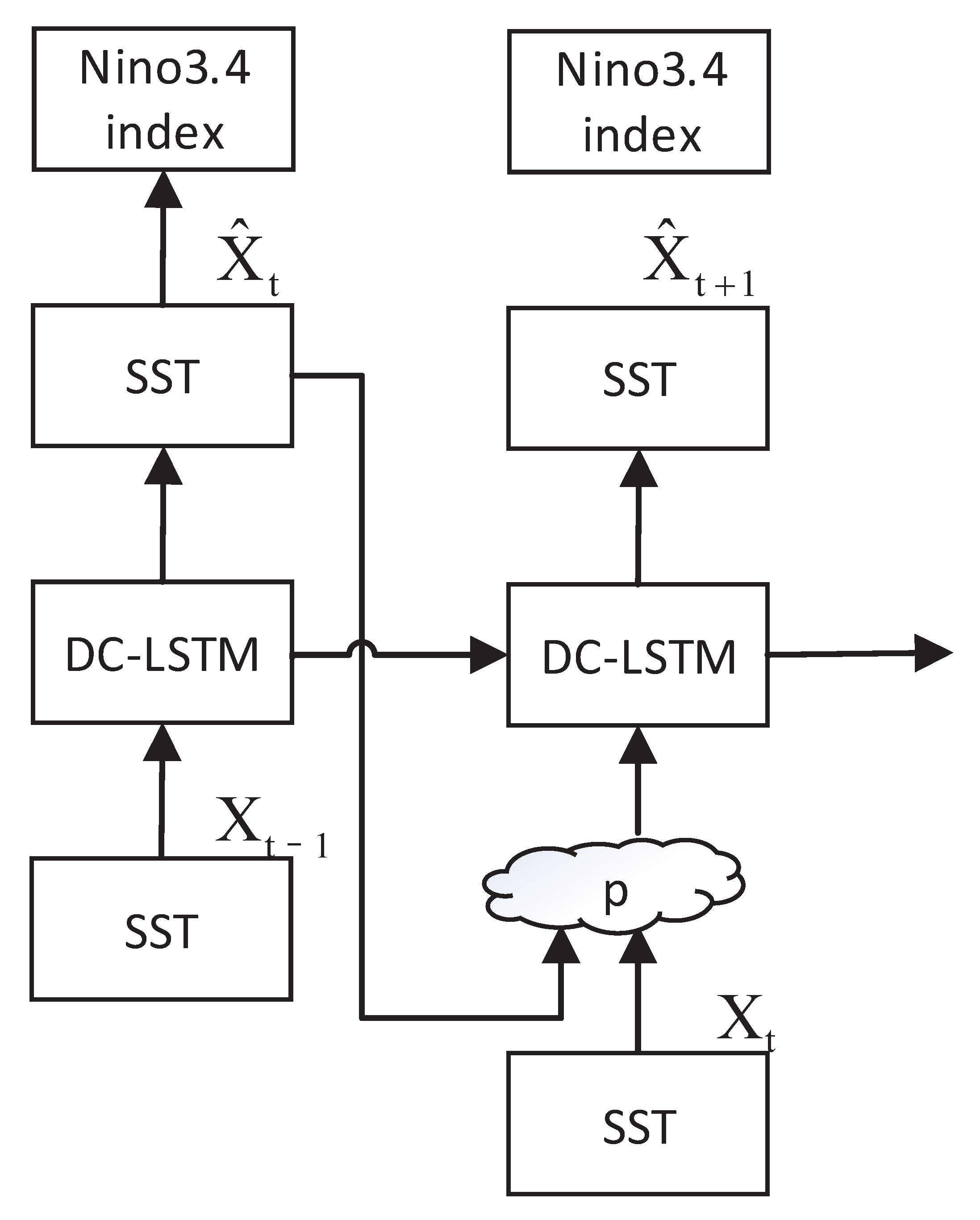
Figure 2 shows the prediction mechanism of the whole system. In the training phase, for the input, probability p is the true value, and probability 1-p is the last prediction. In the initial stage, the prediction ability of the model is weak, and the value of p is 1. With the increase of training iterations, the value of p decreases gradually. In the verification phase, p is fixed to 0. The specific structure of each module is as follows.

2.1. Causal LSTM

In sequence-to-sequence tasks, LSTM [28] has been widely used as a special RNN model. The flow of information in LSTM is controlled by a ‘Gate’ structure, the value of which is between 0 and 1. Among them, the forget gate f t controls the discarding of old features, the input gate i t controls the addition of new features, and the output gate o t controls the output content of the hidden layer. With the help of the gate structure, LSTM has a stable and powerful long-range dependencies modeling capability. It should be noted that, in the original LSTM, the input, output and states must be 1D vectors. The key equations are shown as below, where ‘⊙’ denotes the Hadamard product:
i t = σ W x i x t + W h i h t 1 + W c i c t 1 + b i f t = σ W x f x t + W h f h t 1 + W c f c t 1 + b f c t = f t c t 1 + i t tanh W x c x t + W h c h t 1 + b c o t = σ W x o x t + W h o h t 1 + W c o c t + b o h t = o t tanh c t .
Causal-LSTM [37] is a spatiotemporal memory module based on LSTM. Each Causal-LSTM cell memorizes the spatiotemporal features of the sequence through the state C transferred along the horizontal direction and the state M transferred along the zigzag direction. Like ConvLSTM [38], CausalLSTM extracts spatiotemporal features by replacing the full connections operation with the convolution operator in the state-to-state and input-to-state transitions. Causal-LSTM adopts a cascaded mechanism, where C t will be concatenated with x t , M l to calculate the input gate i t , and the forget gate f t . Finally, the current hidden state h t can be achieved by concatenating C t and M t . The equations of Causal LSTM are shown as follows:
g t i t f t = tanh σ σ W 1 X t , H t 1 k , C t 1 k C t k = f t C t 1 k + i t g t g t i t f t = tan h σ σ W 2 X t , C t k , M t k 1 M t k = f t tanh W 3 M t k 1 + i t g t o t = tanh W 4 X t , C t k , M t k H t k = o t tanh W 5 C t k , M t k ,
where ⊙ is the Hadamard product, * is convolution, σ is Sigmoid activation function, and the superscript K means the layer in the stacked Causal-LSTM network. The square bracket indicates the concatenation operation of the tensors in the channel dimension. W m and W h are 1 × 1 convolutional filters for making the channel number of the concatenation tensor consistent with that of hidden state h t .
For the sea surface temperature anomaly prediction task, the length of input and output sequences is usually above 30. Due to the zigzag transmission route of spatial memory M, the distance is too long for transmitting the early information to the current state. However, these features are important for the prediction of interannual SSTA. Inspired by highway layers [39], a new spatiotemporal recurrent structure, named the Gradient Highway Unit (GHU), was inserted between the bottom and second layers of Causal LSTM. GHU can help the model to learn the capability of skipping frames and make the propagation of the gradient more efficient in very deep feed-forward networks. The equations of GHU are shown below:
P t = tanh W x p X t + W z p Z t 1 S t = σ W x s X t + W z s Z t 1 Z t = S t P t + 1 S t Z t 1 .

2.2. Dense Convolution Layer

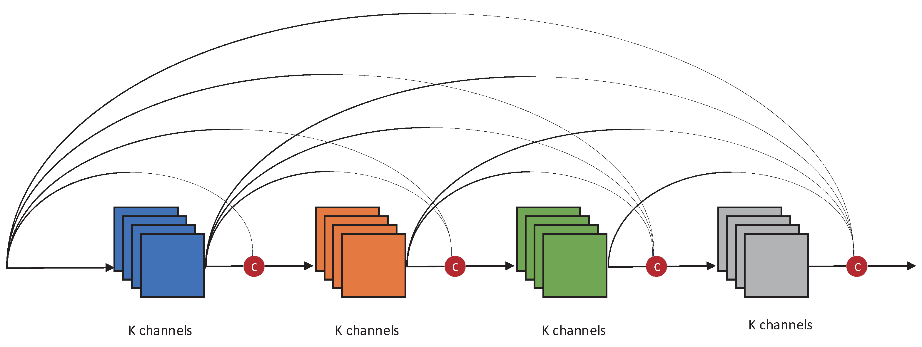
The algorithm using LSTM requires high computation power during its training, which limits the application of a neural network to a certain extent. Therefore, the input needs to be compressed while retaining the key features as much as possible before prediction, and then needs to restore the image size after prediction. Inspired by [40], we tried to use an end-to-end trainable method called Dense Convolution and Transpose Convolution instead of the inflexible patch sampling in the original model. The basic module of the dense convolutional layer is the Dense Block, the structure of which is shown in Figure 3.
In this module, each layer of convolution can receive input from all previous layers and pass its output to all subsequent layers. The cascading method allows each layer to accept the “collective knowledge” from the front:
X l = H l X 0 , X 1 , , X l 1 .
Since the channel concatenation operation requires feature maps of the same size in the block, a translation layer is inserted between adjacent blocks to reduce the feature size. The translation layer is composed of 1 × 1 convolution and max pooling. The max pooling layer only keeps the maximum value in one region of the feature maps (size = 2, stride = 2), and 1 × 1 convolution is used to adjust the shape. In the down sampling stage, the size of the feature map will be reduced by 2 n times, where n is the number of translation layers. The addition of the Dense Convolution layer makes the DC-LSTM have higher computational efficiency and storage efficiency.

3. Results

3.1. Data and Implementation

Our model uses the Simple Ocean Data Assimilation (SODA) reanalysis data [41] from 1871 to 1973 and the outputs of the Coupled Model Intercomparison Project Phase 5 (CMIP5) from 1861 to 2004 as the training set, which simulates the development of ENSO to a certain extent [42]. We only use a single ensemble member for all CMIP5 models to train the DC-LSTM model. We use the Global Ocean Data Assimilation System (GODAS) reanalysis data [43] from 1994 to 2010 as the validation set (Table 1). The number of ensemble members and the period for each Integration CMIP5 model are given in Table 2.
Since a year in the CMIP5 model is solely dependent on the prescribed greenhouse gas forcing, the observational information and the CMIP5 historical simulation are independent of each other. In order to eliminate the possible influence of marine memory in the training period on ENSO in the verification period, we also leave a twenty-year gap between the last year of the training set and the earliest year of the verification set. The predictors of our model include monthly average SSTA, T300, UA, and VA. The resolution of the meteorological map at each time is 5 × 5 , covering the area over 55 S– 60 N, 0 360 E. In order to further increase the amount of data, we use a sliding window with a length of 20 and a step size of 1 to extract samples for each CMIP5 mode output. In order to reduce the strong correlation between adjacent samples caused by the sliding window, all samples will be shuffled. Finally, a training set containing 44,698 sequences is obtained.

3.2. Training

The experiment in this article includes five groups, and the specific plan is as follows:
  • Use six different hyperparameters to preliminarily determine the number of stacked layers and hidden layer states of the network, find the network scale that is most suitable for the SSTA prediction problem, and avoid over-fitting;
  • Determine the best predictor by comparing the effects of using SSTA alone and integrating T300 with U-wind and V-wind, respectively;
  • Compare the ENSO correlation skill of the different prediction regions;
  • Verify the improvement of forecasting skills by using historical simulation data;
  • Compare the ENSO prediction skills for the trained DC-LSTM model with dynamic models and other deep learning models;
We use Root Mean Squared Error (RMSE), Mean Absolute Error (MAE) and Structural Similarity (SSIM) to evaluate the model’s ability to predict SST changes, and use the Pearson Correlation Coefficient of the three-month moving average of the Nino3.4 index (current month and the next two months) to evaluate the model’s ability to predict ENSO. Low RMSE and MSE, and high correlation skills and SSIM represent good forecast ability. The indicators are defined as follows:
RMSE = 1 m i = 1 m y i y ^ i 2
MAE = 1 m i = 1 m | y i y ^ i |
SSIM = 2 μ x μ y + c 1 2 σ x y + c 2 μ x 2 + μ y 2 + c 1 σ x 2 + σ y 2 + c 2
r = i = 1 n X i X ^ Y i Y ^ i = 1 n X i X ^ 2 i = 1 n Y i Y ^ 2 .
All experiments are implemented on Pytorch, and we use Adam [44] as the optimizer with MSE loss. The batch size is set to 16, and the starting learning rate is 10 3 . All models will be trained for 2 epochs on a computer with a single NVIDIA GTX 1080ti GPU. The model consists of 6 layers of LSTM, and each layer of hidden states is 128. The size of zero-padding, stride and convolution kernel in state-to-state and input-to-state are 2, 1 and 5. During the whole training process, the random seed is fixed to 100.

3.3. Results and Discussion

Due to the relatively long training period of the model using LSTM, it is difficult to find the optimal parameters through a large number of trial-and-error experiments. We set some insensitive hyperparameters as fixed values (time steps = 10, kernerl size = 5, stride = 1)—which are widely used in other models using LSTM [35,37,38]—and fine tune others. Table 3 and Table 4 show the RMSE, MSE and SSIM indicators of different hyperparameters for the training set and the test set. We can find that, as the number of layers and hidden states increase, the prediction errors gradually decrease. When the number of layers is six and the number of hidden states is 128, the model achieves the best results on the verification set. It is also worth noting that when the number of layers reaches seven and that of the hidden states reaches 128, the error continues to decline in the training set, but it starts to rebound in the verification set. This suggests that the fitting ability of the model can be improved by increasing the number of parameters, but an excessive fitting training set will affect the generalization performance of the model, that is, the over fitting phenomenon occurs.
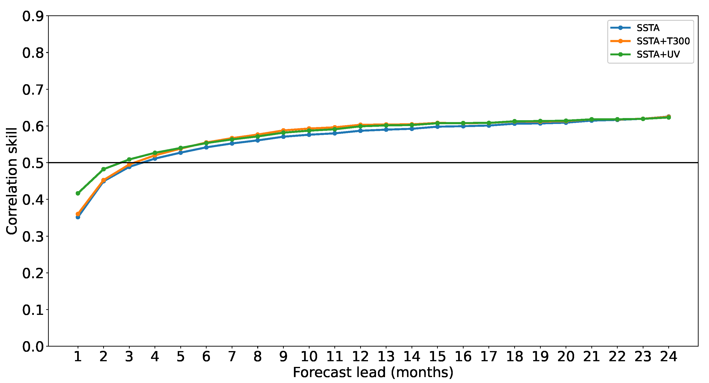
The results of the second experiment are presented in Figure 4 and show that neither the integration of T300 nor the integration of wind field information has brought a lower RMSE, that is, the current DC-LSTM model is temporarily unable to dig out the connections between various meteorological factors. By calculating the correlation coefficients of different factors, we find that the Pearson Correlation Coefficient between SSTA and T300 is too high, reaching 0.741. This suggests that there is a strong linear correlation between SSTA and T300. Therefore, the integration of T300 has no obvious effect on the improvement of accuracy. On the contrary, more feature maps will increase the burden of the model. Considering that the current single factor has the best effect, only SSTA is used as a predictor in subsequent model training.
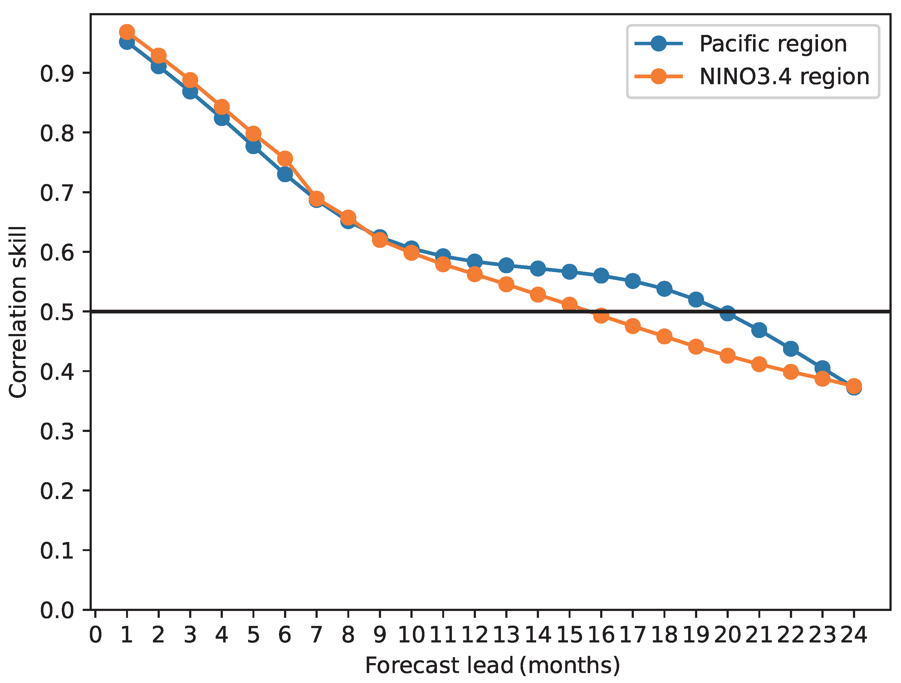
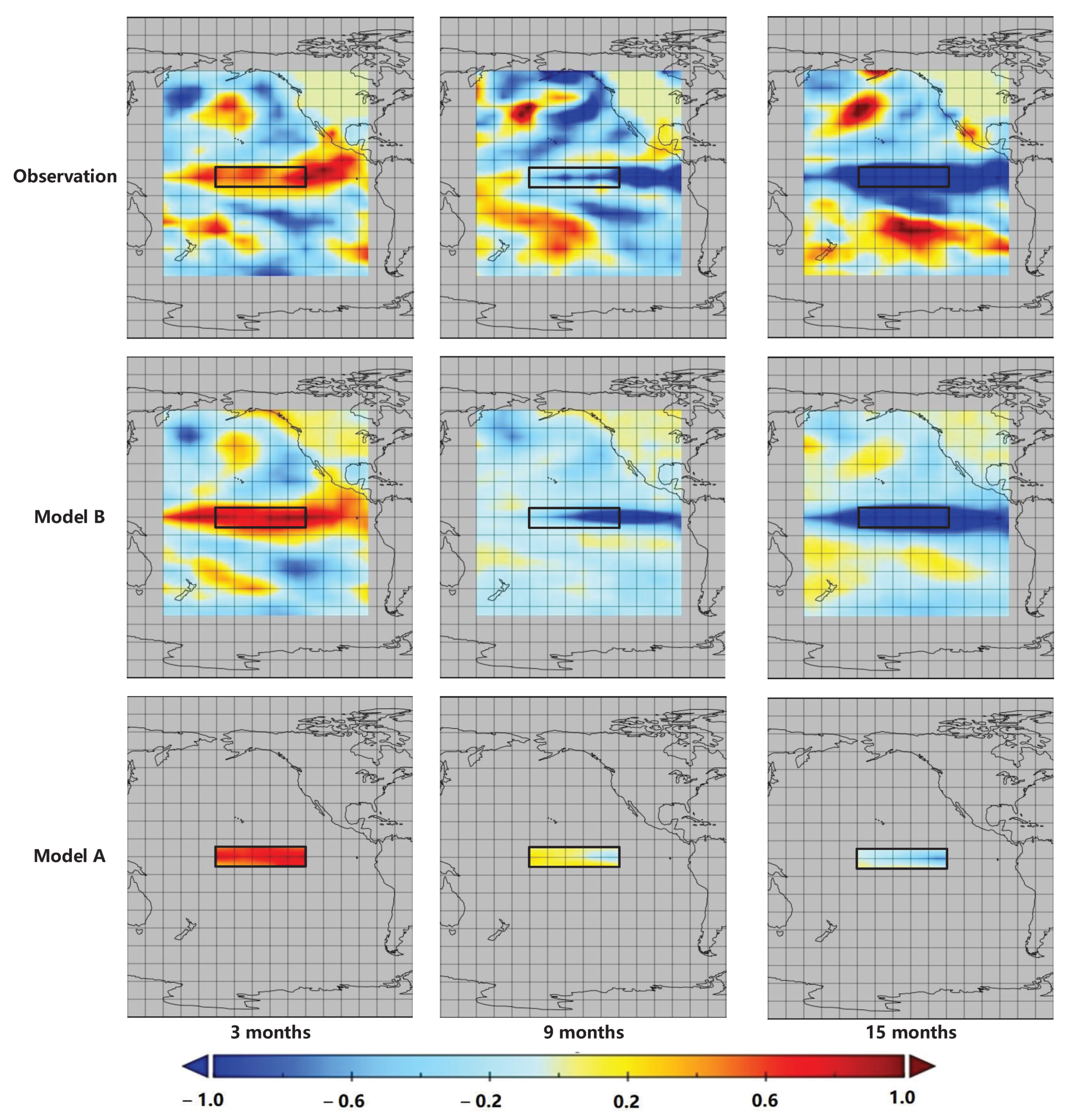
Figure 5 shows the ENSO correlation skills of the models for predicting SSTA in different regions. We can see that model A, which only focuses on the Nino3.4 area, is better at mid and short-term (lead months < 7) prediction, and model B, which focuses on the Pacific area, has stronger long-term prediction (lead months > 7) ability. Figure 6 shows an example of predicting SSTA in different regions. Model A cannot react in advance to the temperature drop in the eastern part of the Nino3.4 area due to its small field of view. On the contrary, model B can capture the sea temperature change from a more macro perspective, so it successfully predicts the trend of sea temperature anomalies over the next 1.5 years.
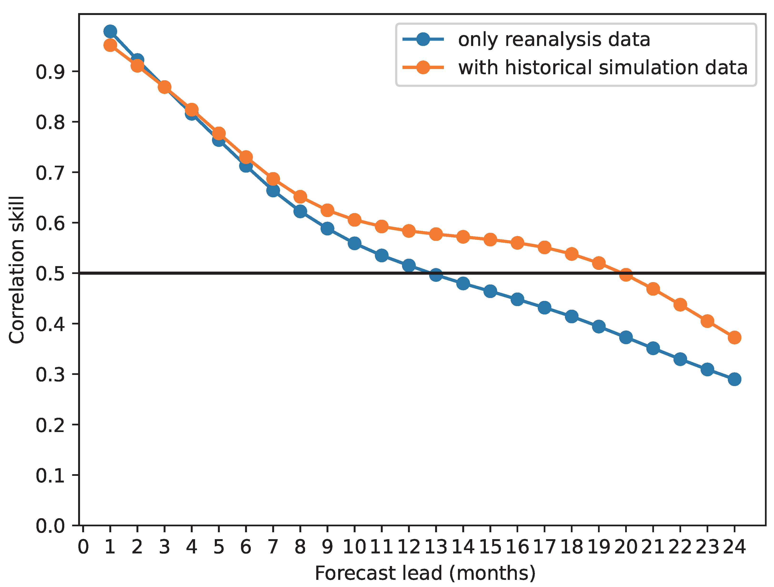
The results for the all-season correlation skills with different datasets are shown in Figure 7. When the model is sufficiently trained, the Nino3.4 index is above 0.5 for a lead time of up to 13 months, whereas it is 0.38 at a lead time of 20 months using only the SODA reanalysis dataset.
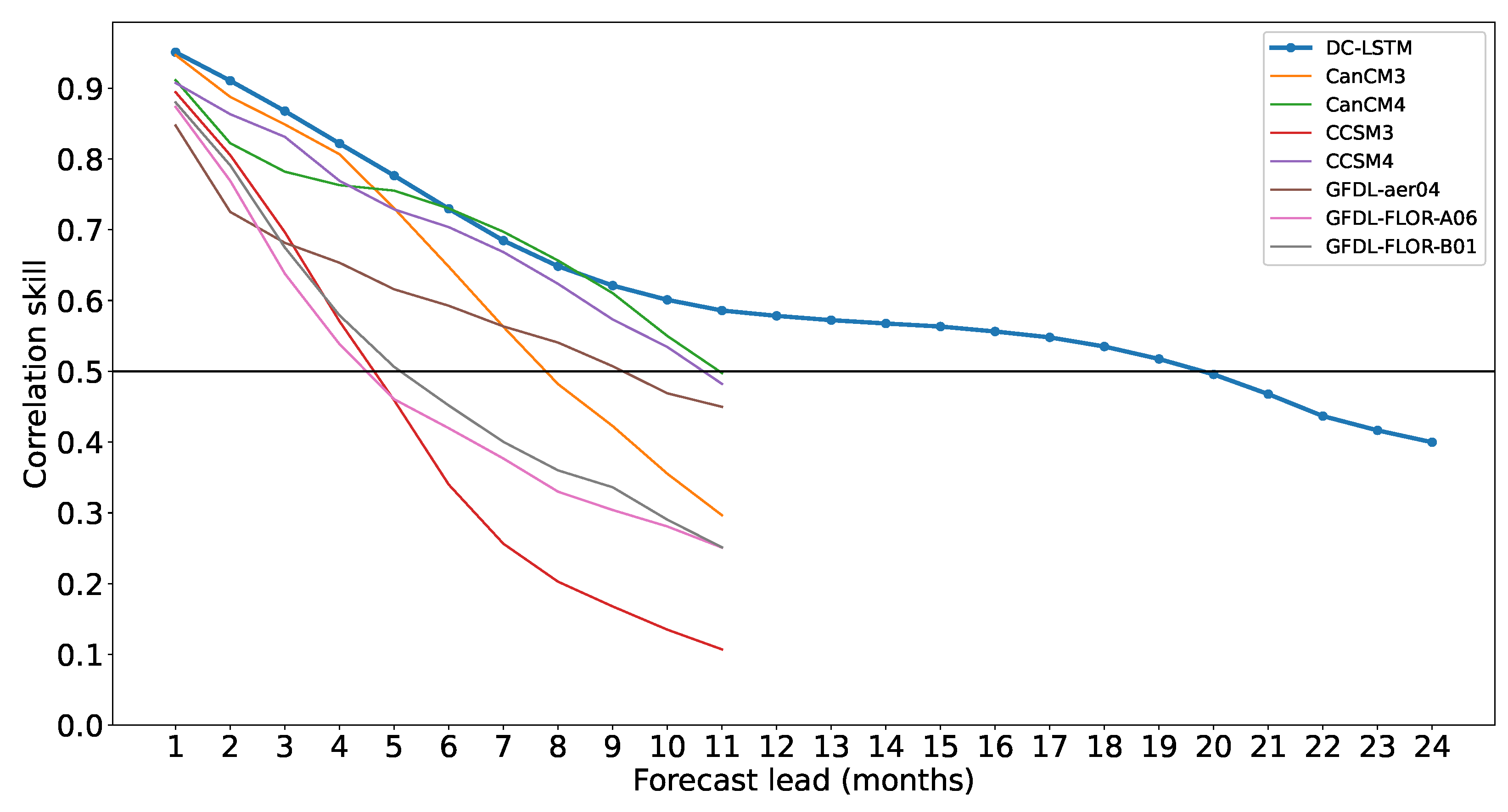
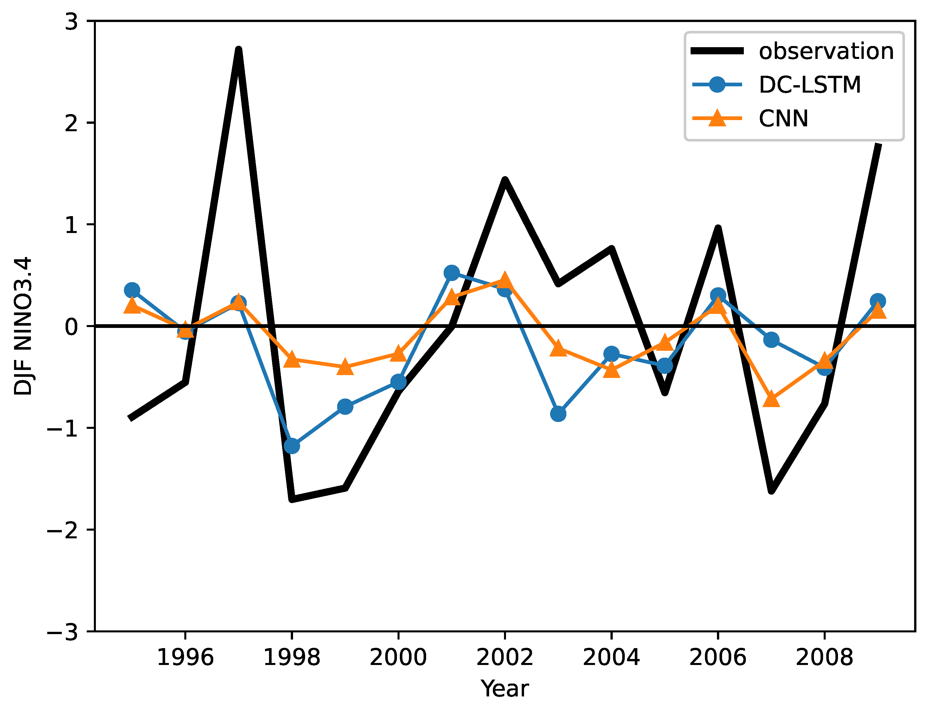
Figure 8 shows the all-season correlation skills of the DC-LSTM model and dynamical models. We use the dynamical prediction systems included in the North American Multi-Model Ensemble (NMME) project as the comparison methods. The NMME dynamical prediction system focuses on forecasting the entire climate state—ocean, atmosphere, land and sea ice—rather than a regional sea surface temperature, so ENSO forecasts for more than 11 months cannot be provided. In the first 11 months, DC-LSTM is one of the two models with the best early forecasting skills. The all-season correlation skills of the DC-LSTM model were higher than 0.5 for 20 months. Table 5 shows that the prediction error of DC-LSTM at a lead time of 20 months is lower than that of CNN. Figure 9 shows the Nino3.4 index of the DC-LSTM and CNN, a leading regression deep learning model [18], for the December–January–February (DJF) season at a lead time of 20 months. We find that CNN and DC-LSTM can approximately predict the trend of the Nino3.4 index, but for some extreme cases (such as 1997 and 2009), the prediction is too conservative. Table 6 shows the number of parameters and the time needed to calculate one sequence. Due to the complex gate mechanism of LSTM, DC-LSTM requires much more computation power than CNN. However, considering that the ENSO prediction interval is relatively low, this cost is still acceptable. As science and engineering continue to advance, the cost will decrease. Finally, we consider that, due to its powerful spatiotemporal feature extraction capabilities and sufficient training with a large amount of simulation data, DC-LSTM can provide effective predictions of ENSO events 1.5 years in advance from the perspective of unsupervised learning and spatiotemporal prediction.

4. Conclusions

In this article, we treat the ENSO prediction problem as an unsupervised spatiotemporal prediction problem and design a DC-LSTM model. By analyzing the prediction results using different hyperparameters, regions and predictors, we determined the final plan. Compared with dynamic methods and regression deep learning methods, DC-LSTM can provide longer effective forecasts. Taking into account the versatility of DC-LSTM, as well as ENSO, we will also try to apply it to the prediction of radar echo, precipitation, humidity and other meteorological factors in the future.

Author Contributions

Conceptualization, T.W.; methodology, T.W.; software, T.W.; validation, T.W.; formal analysis, T.W.; investigation, T.W.; resources, H.G.; data curation, T.W.; writing—original draft preparation, T.W.; writing—review and editing, H.G.; visualization, T.W.; supervision, H.G.; project administration, H.G.; funding acquisition, H.G. All authors have read and agreed to the published version of the manuscript.

Funding

This research was funded by National Key Research and Development Plan under Grant 2017YFC1502104, and National Natural Science Foundation of China under Grant 51977100.

Institutional Review Board Statement

Not applicable.

Informed Consent Statement

Not applicable.

Data Availability Statement

Data related to this paper can be downloaded from: SODA: https://climatedataguide.ucar.edu/climate-data/soda-simple-ocean-data-assimilation (accessed on 1 May 2021); GODAS: https://www.esrl.noaa.gov/psd/data/gridded/data.godas.html (accessed on 1 May 2021); NMME: https://iridl.ldeo.columbia.edu/SOURCES/.Models/.NMME/ (accessed on 1 May 2021); CMIP5: https://esgf-node.llnl.gov/projects/cmip5/ (accessed on 1 May 2021).

Conflicts of Interest

The authors declare no conflict of interest.

References

  1. Bjerknes, J. Atmospheric Teleconnections from the Equatorial PACIFIC1. Mon. Weather Rev. 1969, 97, 163. [Google Scholar] [CrossRef]
  2. Iizumi, T.; Luo, J.J.; Challinor, A.J.; Sakurai, G.; Yokozawa, M.; Sakuma, H.; Brown, M.E.; Yamagata, T. Impacts of El Niño Southern Oscillation on the global yields of major crops. Nat. Commun. 2014, 5, 3712. [Google Scholar] [CrossRef] [PubMed] [Green Version]
  3. Zhai, P.; Yu, R.; Guo, Y.; Li, Q.; Ren, X.; Wang, Y.; Xu, W.; Liu, Y.; Ding, Y. The strong El Niño of 2015/16 and its dominant impacts on global and China’s climate. J. Meteorol. Res. 2016, 30, 283–297. [Google Scholar] [CrossRef]
  4. Bamston, A.G.; Chelliah, M.; Goldenberg, S.B. Documentation of a highly ENSO-related sst region in the equatorial pacific: Research note. Atmos. Ocean 1997, 35, 367–383. [Google Scholar] [CrossRef]
  5. Alexander, M.A.; Matrosova, L.; Penland, C.; Scott, J.D.; Chang, P. Forecasting Pacific SSTs: Linear Inverse Model Predictions of the PDO. J. Clim. 2008, 21, 385–402. [Google Scholar] [CrossRef] [Green Version]
  6. Knaff, J.A.; Landsea, C.W. An El Niño-Southern Oscillation Climatology and Persistence (CLIPER) Forecasting Scheme. Weather Forecast. 1997, 12, 633–652. [Google Scholar] [CrossRef] [Green Version]
  7. Xue, Y.; Leetmaa, A. Forecasts of tropical Pacific SST and sea level using a Markov model. Geophys. Res. Lett. 2000, 27, 2701–2704. [Google Scholar] [CrossRef] [Green Version]
  8. Van Den Dool, H.M. Searching for analogues, how long must we wait? Tellus A 1994, 46, 314–324. [Google Scholar] [CrossRef]
  9. Barnston, A.; Dool, H.; Rodenhuis, D.; Ropelewski, C.; Kousky, V.; O’Lenic, E.; Livezey, R.; Zebiak, S.; Cane, M.; Barnett, T.; et al. Long-Lead Seasonal Forecasts—Where Do We Stand? Bull. Am. Meteorol. Soc. 1994, 75, 2097–2114. [Google Scholar] [CrossRef] [Green Version]
  10. Saha, S.; Moorthi, S.; Wu, X.; Wang, J.; Nadiga, S.; Tripp, P.; Behringer, D.; Hou, Y.T.; Chuang, H.Y.; Iredell, M.; et al. The NCEP Climate Forecast System Version 2. J. Clim. 2014, 27, 2185–2208. [Google Scholar] [CrossRef]
  11. Barnston, A.G.; Tippett, M.K.; L’Heureux, M.L.; Li, S.; DeWitt, D.G. Skill of Real-Time Seasonal ENSO Model Predictions during 2002–11: Is Our Capability Increasing? Bull. Am. Meteorol. Soc. 2012, 93, 631–651. [Google Scholar] [CrossRef]
  12. Luo, J.J.; Masson, S.; Behera, S.K.; Yamagata, T. Extended ENSO Predictions Using a Fully Coupled Ocean—Atmosphere Model. J. Clim. 2008, 21, 84–93. [Google Scholar] [CrossRef]
  13. Tang, Y.; Zhang, R.H.; Liu, T.; Duan, W.; Yang, D.; Zheng, F.; Ren, H.; Lian, T.; Gao, C.; Chen, D.; et al. Progress in ENSO prediction and predictability study. Natl. Sci. Rev. 2018, 5, 826–839. [Google Scholar] [CrossRef]
  14. Mcphaden, M.; Zebiak, S.; Glantz, M. ENSO as an integrating concept in Earth science. Science 2006, 314, 1740–1745. [Google Scholar] [CrossRef] [Green Version]
  15. Kinter, J.L., III; Luo, J.J.; Jin, E.K.; Wang, B.; Park, C.K.; Shukla, J.; Kirtman, B.P.; Kang, I.S.; Schemm, J.; Kug, J.S.; et al. Current status of ENSO prediction skill in coupled ocean-atmosphere models. Clim. Dyn. Obs. Theor. Comput. Res. Clim. Syst. 2008, 31, 647–664. [Google Scholar]
  16. Lima, C.H.R.; Lall, U.; Jebara, T.; Barnston, A.G. Machine Learning Methods for ENSO Analysis and Prediction. In Machine Learning and Data Mining Approaches to Climate Science, Proceedings of the 4th International Workshop on Climate Informatics, Boulder, CO, USA, 25–26 September 2015; Springer International Publishing: Berlin/Heidelberg, Germany, 2015; pp. 13–21. [Google Scholar]
  17. Nooteboom, P.; Feng, Q.; López, C.; Hernández-García, E.; Dijkstra, H. Using network theory and machine learning to predict El Niño. Earth Syst. Dyn. 2018, 9, 969–983. [Google Scholar] [CrossRef] [Green Version]
  18. Ham, Y.G.; Kim, J.H.; Luo, J.J. Deep learning for multi-year ENSO forecasts. Nature 2019, 573, 568–572. [Google Scholar] [CrossRef]
  19. Yosinski, J.; Clune, J.; Bengio, Y.; Lipson, H. How transferable are features in deep neural networks? In Proceedings of the 27th International Conference on Neural Information Processing Systems, Montreal, QC, Canada, 8–13 December 2014; MIT Press: Cambridge, MA, USA, 2014; Volume 2, pp. 3320–3328. [Google Scholar]
  20. Zhang, H.; Chu, P.S.; He, L.; Unger, D. Improving the CPC’s ENSO Forecasts using Bayesian model averaging. Clim. Dyn. 2019, 53, 3373–3385. [Google Scholar] [CrossRef]
  21. Salman, A.G.; Kanigoro, B.; Heryadi, Y. Weather forecasting using deep learning techniques. In Proceedings of the 2015 International Conference on Advanced Computer Science and Information Systems (ICACSIS), Depok, Indonesia, 10–11 October 2015; pp. 281–285. [Google Scholar] [CrossRef]
  22. Soman, S.S.; Zareipour, H.; Malik, O.; Mandal, P. A review of wind power and wind speed forecasting methods with different time horizons. In Proceedings of the North American Power Symposium 2010, Arlington, TX, USA, 26–28 September 2010; pp. 1–8. [Google Scholar] [CrossRef]
  23. Feng, Q.Y.; Vasile, R.; Segond, M.; Gozolchiani, A.; Wang, Y.; Abel, M.; Havlin, S.; Bunde, A.; Dijkstra, H.A. ClimateLearn: A machine-learning approach for climate prediction using network measures. Geosci. Model Dev. Discuss. 2016, 2016, 1–18. [Google Scholar] [CrossRef] [Green Version]
  24. Xie, A.; Yang, H.; Chen, J.; Sheng, L.; Zhang, Q. A Short-Term Wind Speed Forecasting Model Based on a Multi-Variable Long Short-Term Memory Network. Atmosphere 2021, 12, 651. [Google Scholar] [CrossRef]
  25. Aguilar-Martinez, S.; Hsieh, W.W. Forecasts of Tropical Pacific Sea Surface Temperatures by Neural Networks and Support Vector Regression. Int. J. Oceanogr. 2009, 2009, 167. [Google Scholar] [CrossRef] [Green Version]
  26. Zhang, Q.; Wang, H.; Dong, J.; Zhong, G.; Sun, X. Prediction of Sea Surface Temperature Using Long Short-Term Memory. IEEE Geosci. Remote Sens. Lett. 2017, 14, 1745–1749. [Google Scholar] [CrossRef] [Green Version]
  27. Elman, J.L. Finding Structure in Time. Cogn. Sci. 1990, 14, 179–211. [Google Scholar] [CrossRef]
  28. Hochreiter, S.; Schmidhuber, J. Long Short-Term Memory. Neural Comput. 1997, 9, 1735–1780. [Google Scholar] [CrossRef]
  29. Finn, C.; Goodfellow, I.J.; Levine, S. Unsupervised Learning for Physical Interaction through Video Prediction. In Proceedings of the Conference and Workshop on Neural Information Processing Systems, Barcelona, Spain, 5–10 December 2016; pp. 64–72. [Google Scholar]
  30. Brabandere, B.; Jia, X.; Tuytelaars, T.; Van Gool, L. Dynamic Filter Networks. In Proceedings of the Conference and Workshop on Neural Information Processing Systems, Barcelona, Spain, 5–10 December 2016; pp. 667–675. [Google Scholar]
  31. Wang, Y.; Jiang, L.; Yang, M.H.; Li, L.J.; Long, M.; Fei-Fei, L. Eidetic 3D LSTM: A Model for Video Prediction and Beyond. In Proceedings of the 7th International Conference on Learning Representations, New Orleans, LA, USA, 6–9 May 2019. [Google Scholar]
  32. Srivastava, N.; Mansimov, E.; Salakhutdinov, R. Unsupervised learning of video representations using LSTMs. In Proceedings of the International Conference on Machine Learning, JMLR.org, Lille, France, 6–11 July 2015; Volume 37, pp. 843–852. [Google Scholar]
  33. Wang, Y.; Zhang, J.; Zhu, H.; Long, M.; Wang, J.; Yu, P.S. Memory in Memory: A Predictive Neural Network for Learning Higher-Order Non-Stationarity From Spatiotemporal Dynamics. In Proceedings of the IEEE Conference on Computer Vision and Pattern Recognition, Long Beach, CA, USA, 16–20 June 2019; pp. 9154–9162. [Google Scholar]
  34. Kalchbrenner, N.; Oord, A.; Simonyan, K.; Danihelka, I.; Vinyals, O.; Graves, A.; Kavukcuoglu, K. Video Pixel Networks. In Proceedings of the International Conference on Machine Learning, PMLR, Sydney, Australia, 6–11 August 2017; Doina, P., Yee Whye, T., Eds.; Volume 70, pp. 1771–1779. [Google Scholar]
  35. Wang, Y.; Long, M.; Wang, J.; Gao, Z.; Yu, P.S. PredRNN: Recurrent Neural Networks for Predictive Learning using Spatiotemporal LSTMs. In Proceedings of the Conference and Workshop on Neural Information Processing Systems, Long Beach, CA, USA, 4–9 December 2017; pp. 879–888. [Google Scholar]
  36. Shi, X.; Gao, Z.; Lausen, L.; Wang, H.; Yeung, D.; Wong, W.; Woo, W. Deep learning for precipitation nowcasting: A benchmark and a new model. In Proceedings of the Conference and Workshop on Neural Information Processing Systems, Long Beach, CA, USA, 4–9 December 2017; Curran Associates Inc.: Red Hook, NY, USA, 2017; pp. 5622–5632. [Google Scholar]
  37. Wang, Y.; Gao, Z.; Long, M.; Wang, H.; Yu, P.S. PredRNN++: Towards A Resolution of the Deep-in-Time Dilemma in Spatiotemporal Predictive Learning. In Proceedings of the International Conference on Machine Learning, PMLR, Stockholm, Sweden, 10–15 July 2018; Jennifer, D., Andreas, K., Eds.; Volume 80, pp. 5123–5132. [Google Scholar]
  38. Shi, X.; Chen, Z.; Wang, H.; Yeung, D.; Wong, W.; Woo, W. Convolutional LSTM Network: A machine learning approach for precipitation nowcasting. arXiv 2015, arXiv:1506.04214. [Google Scholar]
  39. Srivastava, R.K.; Greff, K.; Schmidhuber, J. Training very deep networks. arXiv 2015, arXiv:1507.06228. [Google Scholar]
  40. Huang, G.; Liu, Z.; Maaten, L.V.D.; Weinberger, K.Q. Densely Connected Convolutional Networks. In Proceedings of the 2017 IEEE Conference on Computer Vision and Pattern Recognition, Honolulu, HI, USA, 21–26 July 2017; pp. 2261–2269. [Google Scholar] [CrossRef] [Green Version]
  41. Carton, J.A.; Giese, B.S. A Reanalysis of Ocean Climate Using Simple Ocean Data Assimilation (SODA). Mon. Weather Rev. 2008, 136, 2999–3017. [Google Scholar] [CrossRef]
  42. Bellenger, H.; Guilyardi, E.; Leloup, J.; Lengaigne, M.; Vialard, J. ENSO representation in climate models: From CMIP3 to CMIP5. Clim. Dyn. 2014, 42, 1999–2018. [Google Scholar] [CrossRef]
  43. Saha, S.; Nadiga, S.; Thiaw, C.; Wang, J.; Wang, W.; Zhang, Q.; Van den Dool, H.M.; Pan, H.L.; Moorthi, S.; Behringer, D.; et al. The NCEP Climate Forecast System. J. Clim. 2006, 19, 3483–3517. [Google Scholar] [CrossRef] [Green Version]
  44. Kingma, D.; Ba, J. Adam: A Method for Stochastic Optimization. arXiv 2015, arXiv:1412.6980. [Google Scholar]
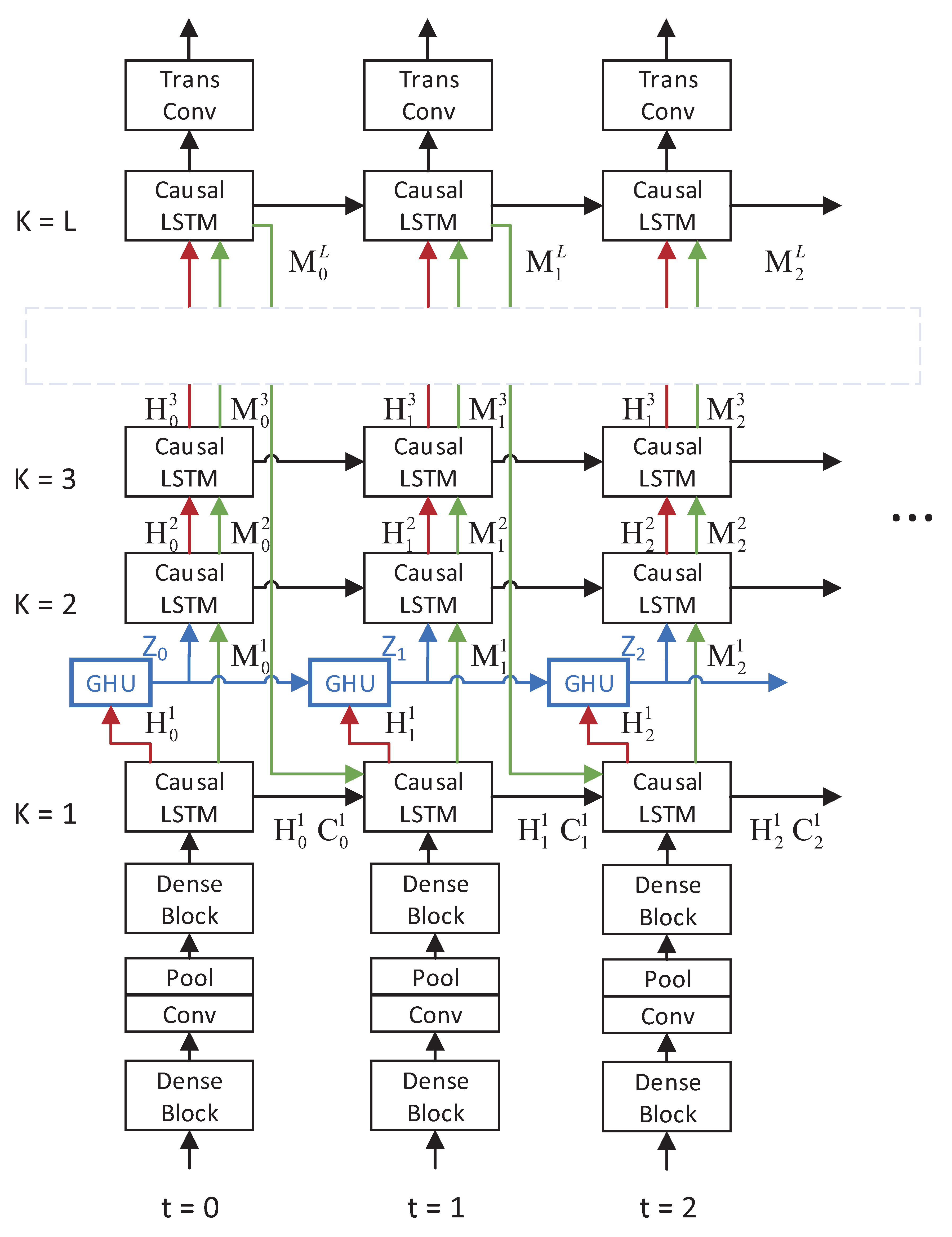
Figure 1. The structure of the DC-LSTM model.
Atmosphere 12 00810 g001
Figure 2. The diagram of the overall system.
Atmosphere 12 00810 g002
Figure 3. Structure of Dense Block.
Atmosphere 12 00810 g003
Figure 4. RMSE comparison of the models with different predictors.
Atmosphere 12 00810 g004
Figure 5. Comparison of the ENSO correlation skill with the different prediction regions.
Atmosphere 12 00810 g005
Figure 6. SSTA regional distribution map with different lead times. Observation represents the real SST, and model A (Nino3.4 area) and model B (Pacific area) represent the predicted SST.
Atmosphere 12 00810 g006
Figure 7. The improvement in the skill of the DC-LSTM model due to the historical simulation dataset.
Atmosphere 12 00810 g007
Figure 8. Comparison of the ENSO correlation skill between the DC-LSTM and dynamic models.
Atmosphere 12 00810 g008
Figure 9. Time series of DJF season Nino3.4 indexes for a 20-month-lead forecast using the CNN model (orange) and the DC-LSTM model (blue).
Atmosphere 12 00810 g009
Table 1. The datasets for training and validating the DC-LSTM model.
DataPeroid
Training datasetCMIP5 historical run1861–2004
Reanalysis (SODA)1971–1973
Validation datasetReanalysis (GODAS)1994–2017
Table 2. Details of the CMIP5 models.
CMIP IDModeling GroupIntegration PeriodNumber of Ensemble Members
BCC-CSM1.1-mBeijing Climate Center, China Meteorological AdministrationJAN1850-DEC20121
CanESM2Canadian Centre for Climate Modelling and AnalysisJAN1850-DEC20055
CCSM4National Center for Atmospheric ResearchJAN1850-DEC20051
CESM1-CAM5Community Earth System Model ContributorsJAN1850-DEC20051
CMCC-CMCentro Euro-Mediterraneo per l Cambiamenti ClimaticiJAN1850-DEC20051
CMCC-CMS1
CNRM-CM5Centre National de Recherches Meteorologiques/Centre Europeen de Recherche et Formation Avancee en Calcul ScientifiqueJAN1850-DEC20055
CSIRO-Mk3-6-0Commonwealth Scientific and Industrial Research Organization in collaboration with Queensland Climate Change Centre of ExcellenceJAN1850-DEC20055
FIO-ESMThe First Institute of Oceanography, SOA, ChinaJAN1850-DEC20051
GFDL-ESM2GNOAA Geophysical Fluid Dynamics LaboratoryJAN1861 -DEC20051
GISS-E2-HNASA Goddard Institute for Space StudiesJAN1850-DEC20055
HadGEM2-AONational Institute of Meteorological Research/Korea Meteorological AdministrationJAN1860-DEC20051
HadCM3Met Office Hadley Centre (additional HadGEM2-ES realizations contributed by Instituto Nacional de Pesquisas Espaciais)DEC1859-DEC20051
HadGEM2-CCDEC1859-NOV20051
HadGEM2-ESDEC1859-NOV20054
IPSL-CM5A-MRInstitut Pierre-Simon LaplaceJAN1850-DEC20051
MIROC5Atmosphere and Ocean Research Institute (The University of Tokyo), National Institute for Environmental Studies, and Japan Agency for Marine-Earth Science and TechnologyJAN1850-DEC20121
MPI-ESM-LRMax-Planck-lnstrtut fur Meteorologie (Max Planck Institute for Meteorology)JAN1850-DEC20053
MRI-CGCM3Meteorological Research InstituteJAN1850-DEC 051
NorESM1-MNorwegian Climate CentreJAN1850-DEC20051
NorESM1-ME1
Table 3. Comparison of models with different layers over 24 prediction steps.
Layer RMSEMAESSIM
TrainingValidationTrainingValidationTrainingValidation
40.57080.58900.40220.40770.570.2863
50.55580.58630.39270.40830.620.2879
60.54190.58580.38330.40820.650.2881
70.53270.59510.37680.41580.660.2849
80.52330.60320.37570.42330.630.2840
Table 4. Comparison of models with different hidden states over 24 prediction steps.
Hidden StatesRMSEMAESSIM
TrainingValidationTrainingValidationTrainingValidation
640.54840.59500.38950.41310.620.2878
1280.54190.58580.38330.40820.650.2881
1920.52170.59560.37210.41420.660.2891
2560.52110.60130.37010.42370.580.2887
Table 5. Quantitative prediction results of different methods at a lead time of 20 months.
ModelCORRMSEMAE
CNN0.62370.56030.4142
DC-LSTM0.65440.55580.3950
Table 6. Comparison of computation power required by different models.
ModelNumber of ParametersTime-Consuming
CNN319,9530.1138 s
DC-LSTM36,130,3040.5145 s
Publisher’s Note: MDPI stays neutral with regard to jurisdictional claims in published maps and institutional affiliations.