Impacts of Climate Change on the Hydrometeorological Characteristics of the Soan River Basin, Pakistan

Abstract

The global hydrological cycle is vulnerable to changing climatic conditions, especially in developing regions, which lack abundant resources and management of freshwater resources. This study evaluates the impacts of climate change on the hydrological regime of the Chirah and Dhoke Pathan sub catchments of the Soan River Basin (SRB), in Pakistan, by using the climate models included in the NEX-GDDP dataset and the hydrological model HBV-light. After proper calibration and validation, the latter is forced with NEX-GDDP inputs to simulate a historic and a future (under the RCP 4.5 and RCP 8.5 emission scenarios) streamflow. Multiple evaluation criteria were employed to find the best performing NEX-GDDP models. A different ensemble was produced for each sub catchment by including the five best performing NEX-GDDP GCMs (ACCESS1-0, CCSM4, CESM1-BGC, MIROC5, and MRI-CGCM3 for Chirah and BNU-ESM, CCSM4, GFDL-CM3. IPSL-CM5A-LR and NorESM1-M for Dhoke Pathan). Our results show that the streamflow is projected to decrease significantly for the two sub catchments, highlighting the vulnerability of the SRB to climate change.

1. Introduction

The hydrological regime of many regions throughout the world has been altered as a consequence of the global climate change [1], with largely different implications depending on the particular location [2].

Very complex relationships exist between the streamflow in a catchment and various climate-related variables such as precipitation, temperature, vapor pressure, and wind speed [3,4,5]. Therefore, a combination of hydrological models and climate simulations from General Circulation Models (GCMs) [6] are typically used to assess the impacts of climate change on the streamflow over a given region.

GCMs are the main tools used nowadays to simulate the evolution of the climate system globally. However, the native spatial resolution of most of the current GCMs is still too coarse to be used in practical applications [6,7]. Therefore, it is common to apply some form of downscaling (either statistical or dynamical downscaling) to translate the coarse-resolution outputs provided by the GCMs to the local-scale required for impact assessment [8,9].

In this context, Sahany et al. [10] showed that the spatial resolution of the GCMs included in the fifth Coupled Model Inter-comparison Project (CMIP5) was too coarse to be used for hydrological modeling at the catchment level. One of the recent advancements to cope with this limitation is the release of the NASA Earth Exchange (NEX) Global Daily Downscaled Projections (GDDP) dataset [11]; dataset URL: (https://www.nccs.nasa.gov/services/data-collections/land-based-products/nex-gddp); accessed on 25 July 2020, a product which provides daily precipitation and temperature for the entire XXI century from an ensemble of 21 GCMs which have been statistically downscaled to cover a high-resolution global grid (0.25°).

This dataset is publicly available and some studies have already used it in different sectors and regions [12,13,14]. Nonetheless, very few studies have focused on the application of NEX-GDDP data for streamflow prediction, especially in Pakistan.

Therefore, the main goal of the present work is to assess the suitability of the NEX-GDDP dataset to be used for hydrological modeling and assessment of climate change impacts on the streamflow of two sub catchments (Chirah and Dhoke Pathan, with different characteristics) of the Soan River Basin (SRB) in Pakistan. The sections of this paper are organized as follows: the study area, data sets, description of hydrological model, and methodologies are given in Section 2; evaluation of the hydrological model’s performance, the performance of GCMs in reproducing historic climate and streamflow, impacts of climate change on future streamflow and climate are described in Section 3; Section 4 consists of the discussion; and the conclusions are summarized in Section 5.

2. Materials and Methods

2.1. Study Area

This study is conducted over two sub catchments of the Soan River Basin (SRB), namely Chirah and Dhoke Pathan (Figure 1), which have a drainage area of 336 km² and 6542 km², respectively. The Soan River has a length of 272 km, and rocks of tertiary age prevail in most of the basin [15], whose elevation ranges from 264 masl to 2274 masl (Figure 1). The climate of this region is categorized as “Sub-tropical Triple Season Moderate Climate Zone”. On average, the temperature is 13.2 °C (17.6 °C), the annual precipitation is 1480 mm (1310 mm), and the streamflow is 345 mm (214 mm) over Chirah (Dhoke Pathan). Both sub catchments are predominately rainfed. However the streamflow in Chirah is influenced by snowmelt as well. While Chirah sub catchment lies along the Himalayan subtropical pine forest and western Himalayan subalpine conifer forest (which are the major terrestrial ecoregions of western Himalayas), Dhoke Pathan sub catchment encounters northwestern thorn scrub forests and comprises the xeric shrubland ecoregion of Pakistan. On the one hand, Chirah sub catchment is located upstream of the river and presents by distinctive topographical features of lower Himalayan foothills i.e., hilly terrain along with many valleys and steep gradient. On the other hand, Dhoke Pathan sub catchment lies downstream of the river and is comprised of hills of low elevations and plateaus. Deep gullies and gorges play a key role in the composition of wasted land as a main land use in the region along with rainfed agriculture [16].

The Soan River is the major source of water and serves the domestic needs of more than 4.5 million residents of Islamabad (capital city of Pakistan) and the city of Rawalpindi. Agricultural activities depend on precipitation and perennial flows. The most important crops of the SRB are wheat, groundnut, millets, oilseeds, fodders, and so forth. Non-calcareous soil type of alluvial and loess plains dominate the basin. Slightly more than fifty percent of the region has flat to gentle slopes, more than twenty percent is comprised of medium slope, and the remaining area has either steep or very steep slopes. Humid and subhumid climates dominate the northern part of the SRB, while southern regions are dominated by arid and semiarid climates [17].

In recent years, a surge in migration from rural to urban areas has significantly increased the population of the study region, which implies that water resources are at a constant threat. Moreover, the aquatic and terrestrial ecosystems of the region have also been affected adversely.

2.2. Historical Observations

On the one hand, historic daily precipitation and temperature data for two gauge stations (Murree and Islamabad) located in the basin (Figure 1) were obtained from the Pakistan Meteorological Department (PMD) for the period 1980–2015. On the other hand, the observed monthly streamflow data for the Soan River at the Chirah and Dhoke Pathan gauge stations were obtained from the Surface Water Hydrology Project (SWHP) of the Water and Power Development Authority (WAPDA) for the period 2001–2015. The Digital Elevation Model (DEM) of 30 m resolution from the Shuttle Radar Topographic Mission (SRTM) was used for the delineation of the sub catchments using ArcGIS 10.2.

2.3. Future Climate Change Projections

Twenty one GCMs from the NEX-GDDP dataset, run under the RCP 4.5 and 8.5 emission scenarios were considered in this study. These models have been bias-corrected by means of the Spatial Disaggregation (BCSD) method [11,18,19,20], using as observational reference the gridded Global Meteorological Forcing Dataset (GMFD) of the Terrestrial Hydrology Research Group at the Princeton University [21]. Thrasher et al. [11] provides an in depth description about NEX-GDDP and the BCSD method that has been utilized to generate the dataset, which provides daily outputs along the entire XXI century on a high resolution (0.25°) global grid. All the twenty one models of the NEX-GDDP dataset, whose details are given in Table S1 (“Supplementary Materials” section), are employed in this work.

2.4. Hydrological Modeling: The HBV-Light Model

The Hydrologiska Byråns Vattenbalansavdelning (HBV) model [22,23] is a semi distributed and conceptual hydrological model. In comparison with other data intensive models (e.g., fully distributed models), a key advantage of semi distributed models is that they can run with less input data.

A modified version of the HBV model is known as HBV-light [24] and has been used in this study to simulate streamflow. It has snow, soil, response, and routing routines. In a first phase, the representation of water flowing is achieved by processing precipitation with respect to a suitable threshold temperature. In the next phase, the soil routine is used in order to process precipitation according to the water content of soil box. Then the response routine becomes active and groundwater recharge adds up to the groundwater box (upper), and percolation is initiated to the groundwater box (lower). Streamflow is then simulated, and in the routing routine, the transport of generated streamflow is represented along the stream network by the application of a triangular weighing function. HBV-light uses temperature, precipitation, and potential evaporation values as driving variables. We refer the interested reader to previous existing literature for a detailed description of the model [9,22,23,24,25,26].

2.5. Calibration and Validation of HBV-Light

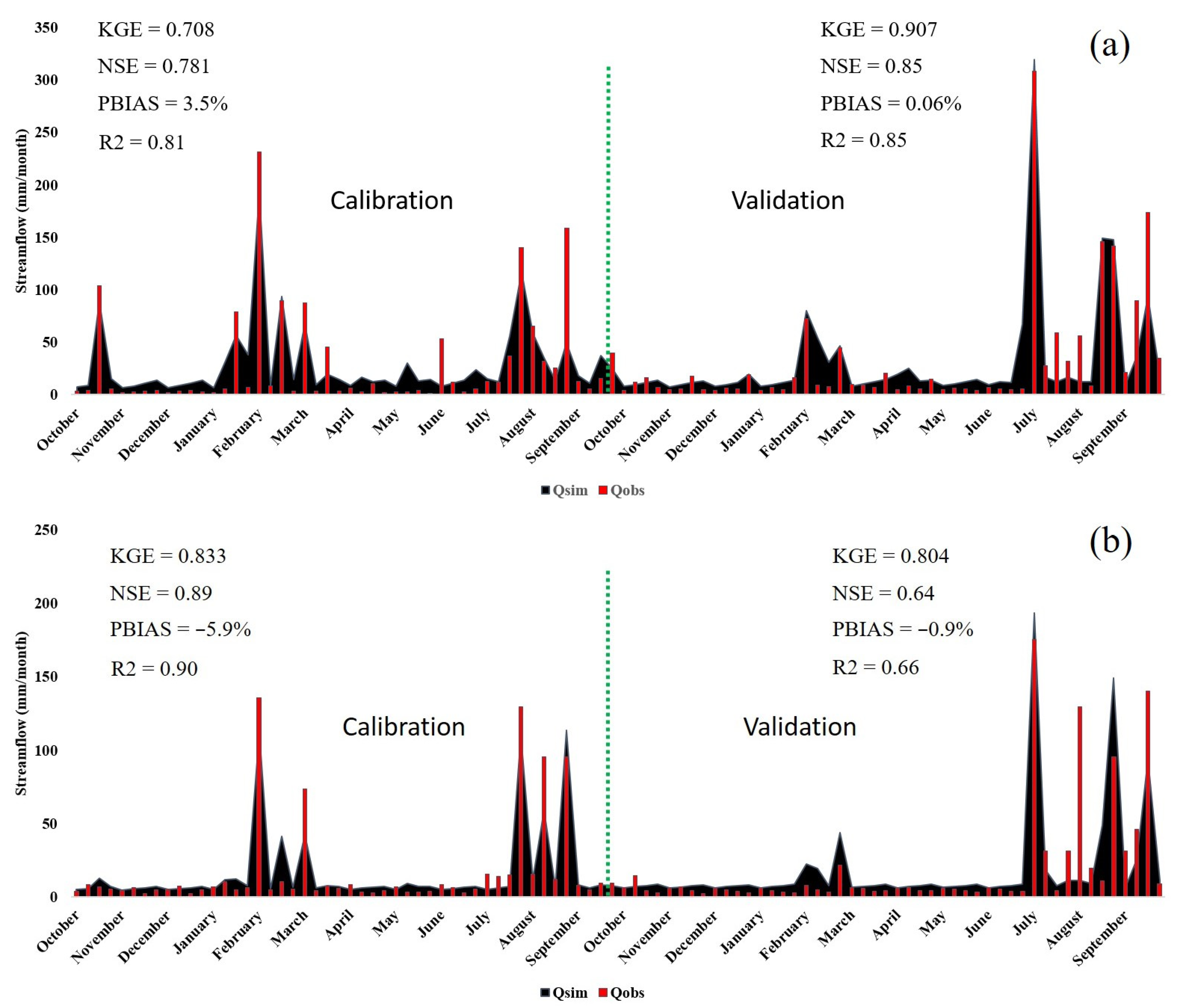
The period 2001–2013 (common to all observed data: precipitation, temperature, and streamflow) was selected for calibration and validation of the HBV-light model. In particular, HBV-light was independently calibrated for the period 2002–2006 (with one year (2001) as spin up period) for Chirah and Dhoke Pathan sub catchments at a monthly scale (i.e., different model parameters were obtained for each sub catchment). After calibration, it was validated for the 2009–2013 period. These two periods correspond to different streamflow episodes over the studied region (e.g., high flow, low flow, and average flow) which allows therefore to robustly test the power of generalization of the model in previously unseen conditions. Different evaluation metrics were used to assess the performance of the model in simulating the observed streamflow during the calibration and validation periods. These metrics include the coefficient of determination ($R^2$), the Nash Sutcliffe Efficiency ($NSE$) [27], the Kling Gupta Efficiency ($KGE$) [28], and the percent bias ($PBIAS$).

Good (poor) model performance is acknowledged for $R^2$, $NSE$, and $KGE$ values between 0.6 and 1 (below 0.4), while optimum value for $PBIAS$ between the observed and modeled streamflow is 0.

$$R^2=\frac{{\left({{\displaystyle \sum }}^{\text{}}\left(Q_{obs}-\overline{Q_{obs}}\right)\left(Q_{sim}-\overline{Q_{sim}}\right)\right)}^2}{{{\displaystyle \sum }}^{\text{}}{\left(Q_{obs}-\overline{Q_{obs}}\right)}^2{{\displaystyle \sum }}^{\text{}}{\left(Q_{sim}-\overline{Q_{sim}}\right)}^2}$$

(1)

$$NSE=1-\frac{{{\displaystyle \sum }}^{\text{}}{\left(Q_{obs}-Q_{sim}\right)}^2}{{{\displaystyle \sum }}^{\text{}}{\left(Q_{obs}-\overline{Q_{obs}}\right)}^2}$$

(2)

$$KGE=1-\sqrt{{\left(r-1\right)}^2+{\left(\alpha -1\right)}^2+{\left(\beta -1\right)}^2}$$

(3)

$$PBIAS=\frac{{{\displaystyle \sum }}_{i=1}^n{s}_i-o_i}{{{\displaystyle \sum }}_{i=1}^n{o}_i}\times 100$$

(4)

$Q_{obs}$ and $Q_{sim}$are the observed and modeled streamflow, $\overline{Q_{obs}}$ and $\overline{Q_{sim}}$ are the observed and modeled mean streamflow, whereas $s$ and $o$ also represent the modeled and observed streamflow.

In Equation (3), r represents the Pearson’s correlation coefficient, the bias (variability) component α (β) is represented by the ratio of modeled and observed means (coefficients of variation).

2.6. Selection of the Best Performing GCMs

The selection of best performing NEX-GDDP GCMs for the Chirah and Dhoke Pathan sub catchments is described in this section.

Precipitation from all the twenty-one NEX-GDDP GCMs was first compared to the historic values on the basis of different criteria (similarity in the number of rainy days, standard deviation, mean and extreme values, etc.). Subsequently, the streamflow for the historic period 1980–2004 was simulated by forcing the HBV-light with osberved (gauge-based) and modeled (NEX-GDDP) climate data. Then, projections of the streamflow for the mid and far future (2040–2064 and 2074–2098, respectively) were obtained by forcing the HBV-light model with the NEX-GDDP GCMs under the RCP 4.5 and RCP 8.5 emission scenarios.

To quantify the similarity between the observed and simulated (i.e., obtained from the HBV-light model based on observed and NEX-GDDP climate inputs) streamflow over the historic period, the correlation coefficient (R²) and the percent bias PBIAS (%) were considered. Moreover, in an effort to minimize the errors associated with future streamflow projections, the volumetric change VC (%) between the historic (that simulated by HBV-light for the historic period based on the observed climate variables) and projected streamflow was also considered.

To assess the suitability of the NEX-GDDP GCMs for projecting the streamflow, a set of efficiency metrics used in previous studies was considered [29,30]. Recall that the HBV-light model was independently calibrated and validated for Chirah and Dhoke Pathan sub catchments; therefore, different threshold values were considered for these three metrics ($R^2$, $PBIAS$, and VC) for both sub catchments in order to select the best performing NEX-GDDP GCMs forming the final multi-model ensemble. In particular, for Chirah sub catchment, we selected the GCMs showing an $R^2$ greater than 0.67, $PBIAS$ below 40% (in absolute value), and VC below 35% (in absolute value). Differently, for Dhoke Pathan sub catchment, we selected the GCMs exhibiting an $R^2$ greater 0.75 and $PBIAS$ and VC below 15% (in absolute value). The models satisfying the aforementioned criteria (which were defined according to previous works by [30,31] and were averaged to form a multi-model ensemble mean, which was ultimately used to feed the HBV-light model in order to simulate future streamflow for 2040–2064 and 2074–2098.

3. Results

3.1. Calibration and Validation

Results for the different metrics used to evaluate the HBV-light’s efficiency during the calibration and validation periods for the Chirah and Dhoke Pathan sub catchments are shown in Figure 2 (Dotted line in green separates the calibration and validation periods). On the one hand, $KGE$ 0.7, $NSE$ 0.78, $PBIAS$ 3.5%, and $R^2$ 0.81 ($KGE$ 0.9, $NSE$ 0.85, $PBIAS$ 0.06%, and $R^2$ 0.85) were achieved during calibration (validation) for Chirah sub catchment. On the other hand, $KGE$ 0.83, $NSE$ 0.89, $PBIAS$ −5.9%, and $R^2$ 0.9 ($KGE$ 0.8, $NSE$ 0.64, $PBIAS$ −0.9%, and $R^2$ 0.66) were achieved during calibration (validation) for the Dhoke Pathan sub catchment. Overall, these results reflect the high performance of the HBV-light model to simulate the monthly streamflow over the region of study.

3.2. NEX-GDDP Models’ Performance in Simulating Observed Climate and Streamflow over Chirah and Dhoke Pathan Sub Catchments

Daily precipitation simulated by all NEX-GDDP GCMs was compared against the corresponding historic (gauge-based) values for both sub catchments over the period 1980–2004 in terms of different indicators: average daily precipitation, average daily maximum precipitation, standard deviation and average number of days which receive more than 1 mm of precipitation.

As shown in Table S2 (“Supplementary Materials” section), in the Chirah sub catchment, all NEX-GDDP GCMs underestimated the average daily precipitation, most of the models also underestimated the maximum daily precipitation except MPI-ESM-MR, MRI-CGCM3, and NorESM1-M. In addition, many models overestimated the number of wet days except CCSM4, CESM1-BGC, and CSIRO-Mk3-6-0. All models overestimated the historic standard deviation as well.

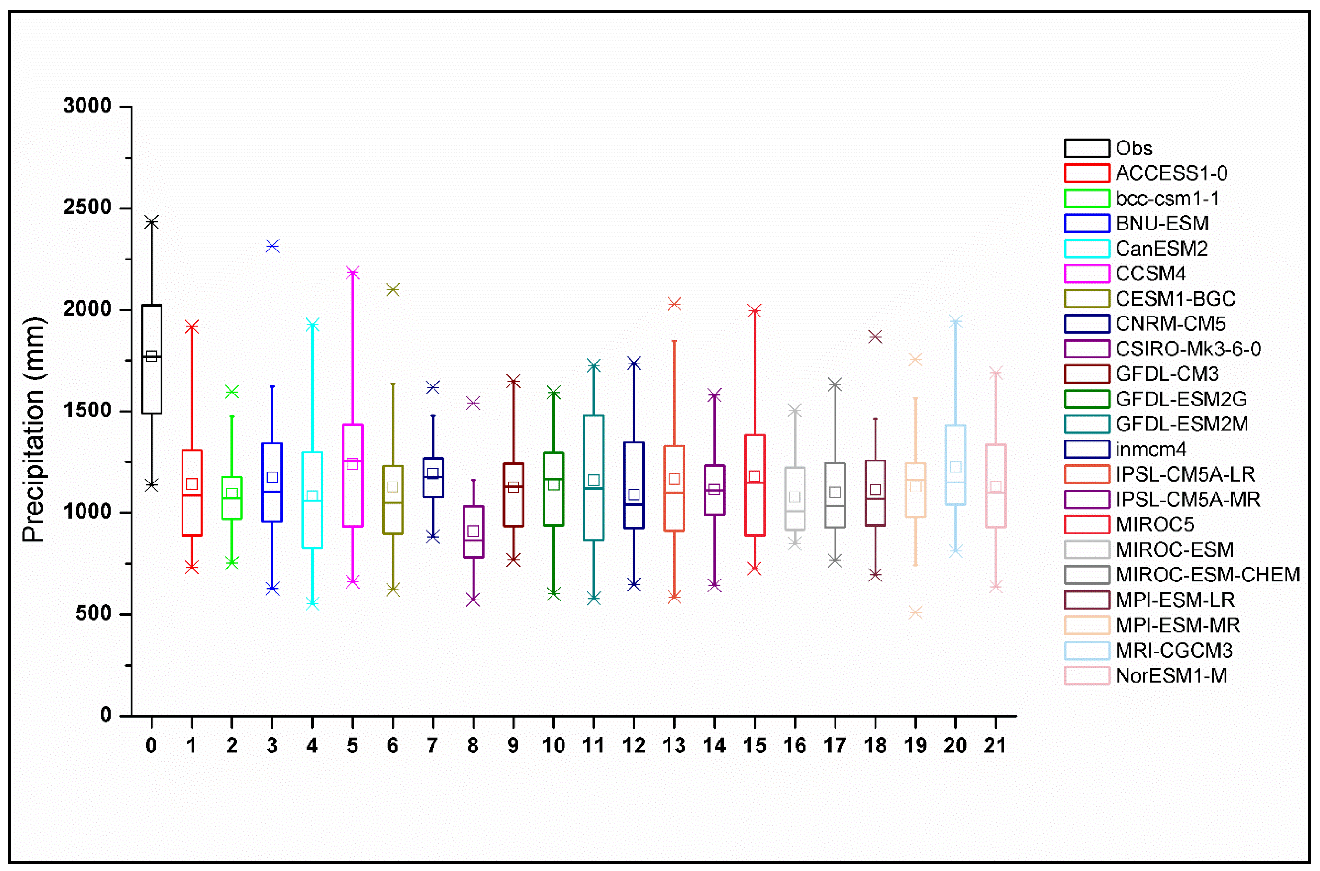
The box plots in Figure 3 show the distribution of historic annual precipitation (in black) over Chirah sub catchment for 1980–2004, together with the corresponding estimations provided by the 21 NEX-GDDP models (in colors). Considerable variability is depicted by almost all the NEX-GDDP GCMs in simulating average annual precipitation.

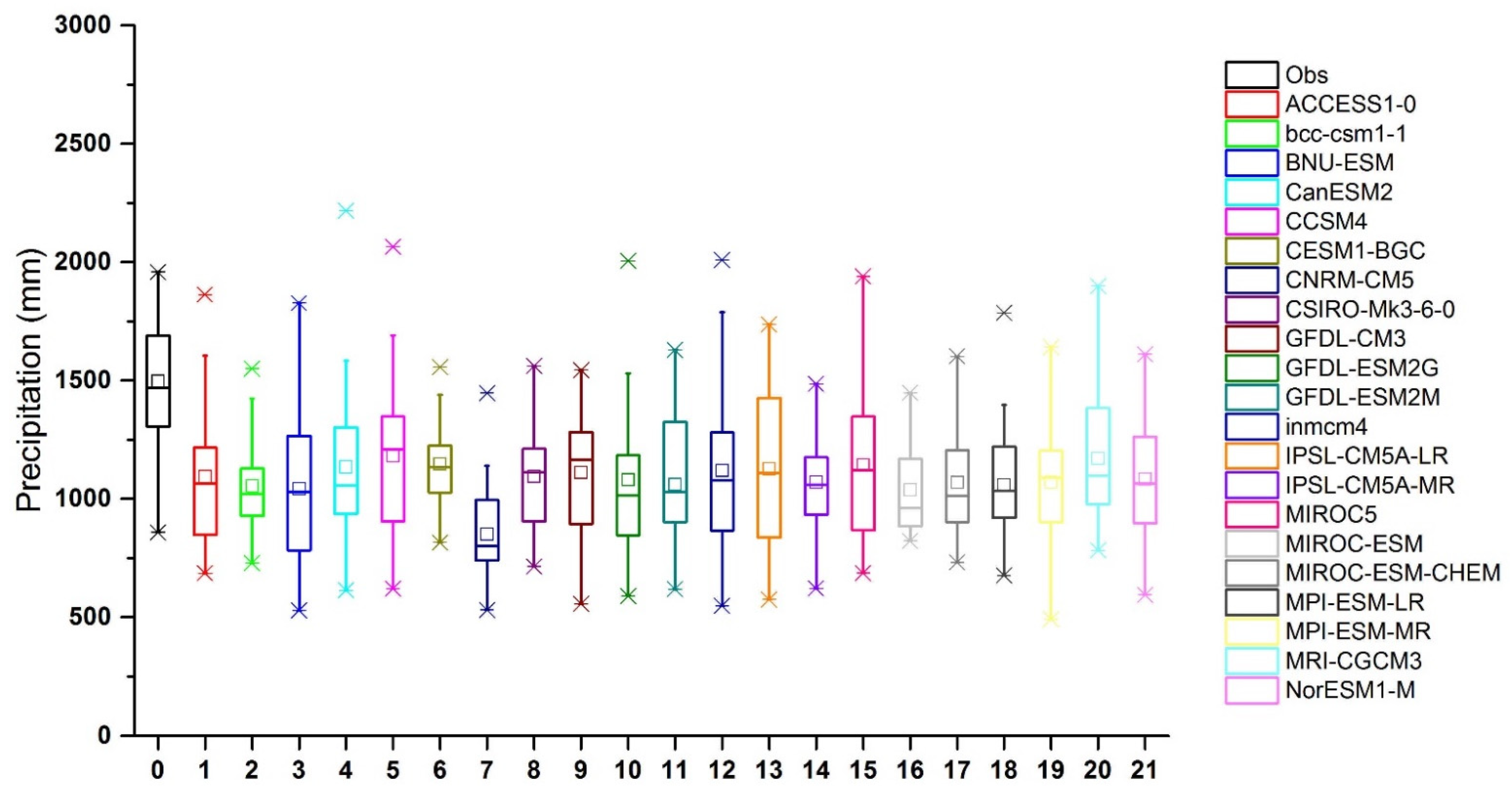
As for Chirah sub catchment, all the NEX-GDDP GCMs were found to underestimate the average daily precipitation over the Dhoke Pathan sub catchment (see Table S3 in the “Supplementary Materials” section). However, higher variability across the different models was detected in terms of maximum daily precipitation and number of wet days in this case. For instance, seven models overestimated the daily maximum precipitation and the number of wet days in Dhoke Pathan sub catchment (Figure 4). A considerable variability is depicted by almost all the NEX-GDDP GCMs in simulating the average annual precipitation.

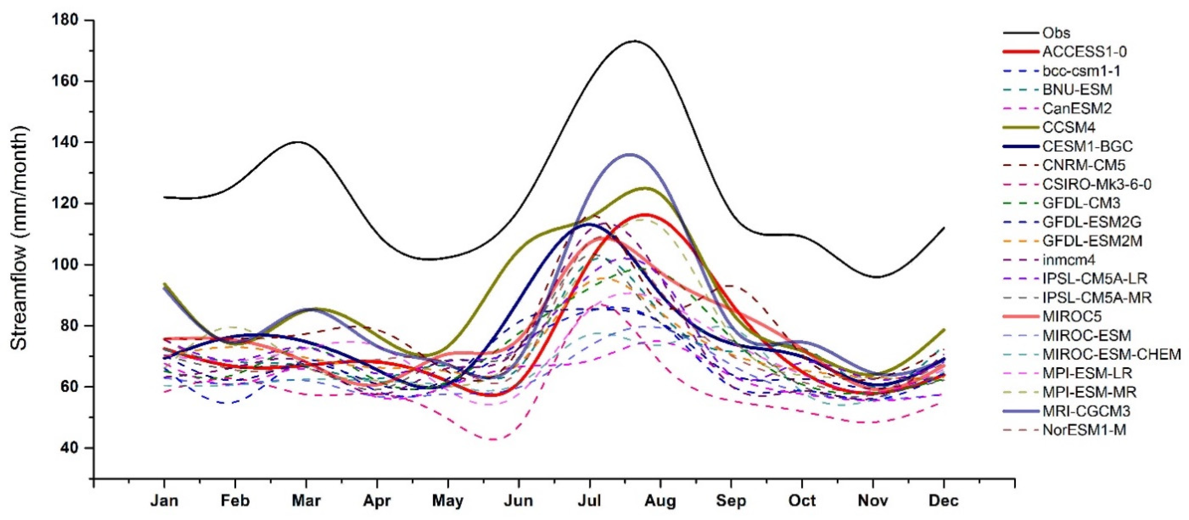
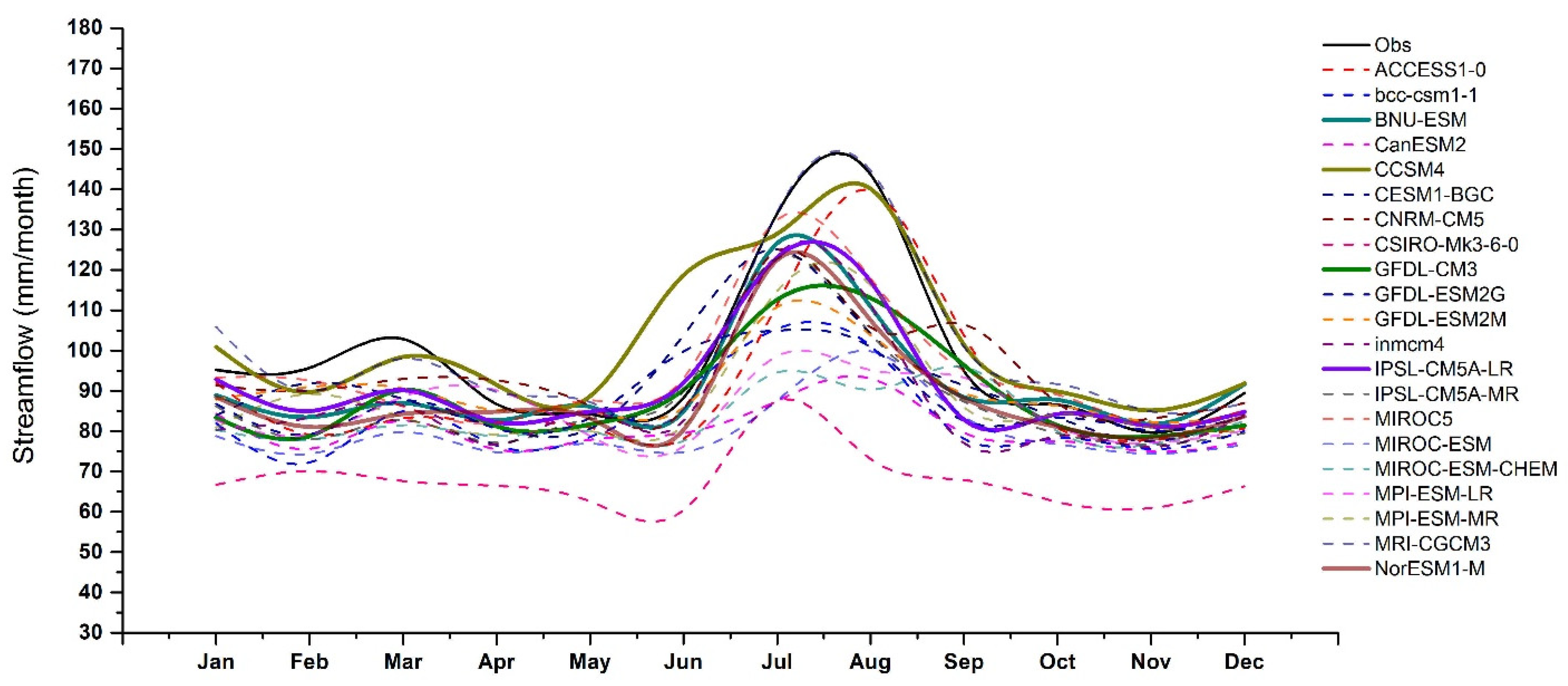
The suitability of the 21 NEX-GDDP GCMs for hydrological modeling was first evaluated by forcing the HBV-light model to simulate historic streamflow over the Chirah and Dhoke Pathan sub catchments for the period 1980–2004 (Figure 5 and Figure 6). For Chirah sub catchment, all the NEX-GDDP GCMs underestimated monthly streamflow with $PBIAS$ values of up to −53%. A high variability across the different GCMs was found in terms of $R^2$ as well, ranging from 0.42 to 0.87.

In Dhoke Pathan sub catchment, the historic streamflow simulated by most of the NEX-GDDP GCMs also underestimated the historic streamflow values, but to a lesser extent. Unlike in Chirah sub catchment, there were a few GCMs (e.g., CCSM4 and MRI-CGCM3) showing an overestimated pattern. A high variability was found across the different GCMs in terms of $R^2$, ranging from 0.47 to 0.94.

On the basis of these results, only those models which satisfied the criteria mentioned in Section 2.6 were selected to form the final multi-model ensemble: ACCESS1-0, CCSM4, CESM1-BGC, MIROC5 and MRI-CGCM3 (BNU-ESM, CCSM4, GFDL-CM3. IPSL-CM5A-LR and NorESM1-M) for the Chirah (Dhoke Pathan) sub catchment. Note that all these models characterized well the interannual variability of the historic streamflow (Figure S1 in the “Supplementary Materials” section).

3.3. Projected Changes in Temperature and Precipitation for the Chirah Sub Catchment

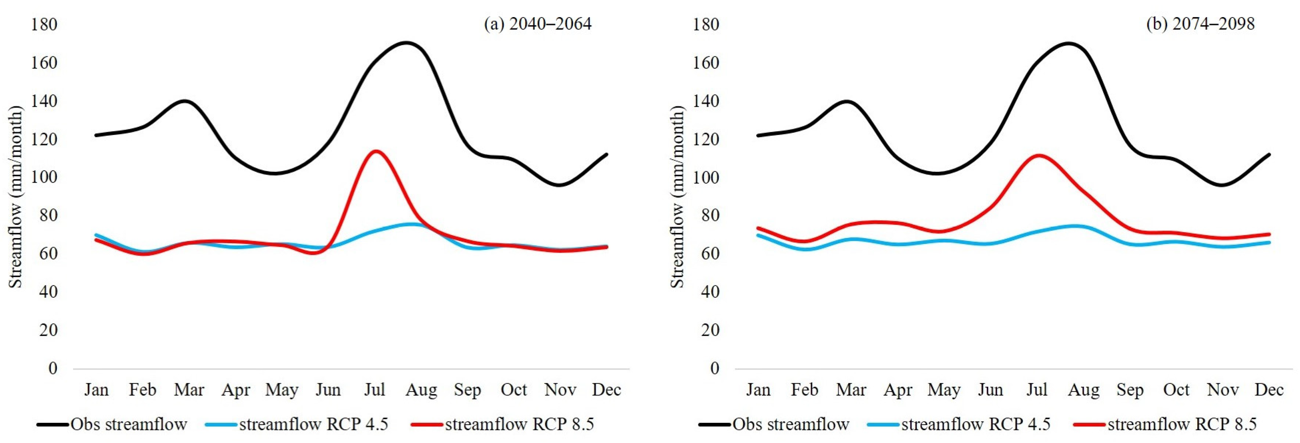
Mean monthly temperature and precipitation for the Chirah sub catchment projected by the multi-model ensemble mean of five selected NEX-GDDP GCMs under the RCP 4.5 and 8.5 emission scenarios for two periods (2040–2064) and (2074–2098) were compared to the corresponding historic values (Figure S2 in the “Supplementary Materials” section). Under both the average (RCP 4.5) and extreme (RCP 8.5) emission scenarios, a rise in temperature is projected over Chirah sub catchment throughout the year for mid and far future periods. However, the magnitude of increase in temperature is slightly higher under the RCP 8.5 emission scenario, i.e., 28.4 °C as compared to 26.4 °C under the RCP 4.5 emission scenario. With regards to precipitation, the future projections given by the multi-model ensemble mean of selected models indicate a considerable decrease (up to 40%) for mid and far future periods under both emission scenarios. Moreover, less precipitation is projected in dry months (winter and early spring) as compared to wet (summer) months. July was the wettest month during the historic period, and this pattern was preserved in the future projections under both emission scenarios as well but with a smaller magnitude. The driest conditions in the Chirah sub catchmentwere observed during the month of November in the historic period, and November remained the driest month (with more intensive dry conditions) in future projections as well.

3.4. Climate Change Impacts on Streamflow for the Chirah Sub Catchment

An increase (decrease) in temperature (precipitation) was projected for mid and far future periods in Chirah sub catchment. These changes can alter the hydrological regime. The HBV-light model was forced with the best performing NEX-GDDP models under both emission scenarios to project streamflow for the Chirah sub catchment (Figure 7). Our results show that the streamflow is projected to decrease for mid and far future periods by up to 47% and 44% under the RCP 4.5 and RCP 8.5 emission scenarios, respectively. The reduction in the volume of the streamflow throughout the year under RCP 4.5 indicates that the wet season in the historic period is expected to shift towards drier conditions, and drier conditions in the historic period are projected to undergo further intensification in future. The peak streamflow was attained in the month of August in the historic period, and it is expected to shift backward towards July according to our future projections. As compared to RCP 4.5, a high interannual variability is projected under the RCP 8.5 emission scenario over Chirah sub catchment (Figure S4 in the “Supplementary Materials” section).

3.5. Projected Changes in Temperature and Precipitation for the Dhoke Pathan Sub Catchment

The mean monthly temperature and precipitation projected under both emission scenarios over Dhoke Pathan sub catchment by the multi-model ensemble mean of five selected NEX-GDDP GCMs for these two periods (2040–2064) and (2074–2098) were compared to the corresponding historic values (Figure S3 in “Supplementary Materials” section). Under both emission scenarios, the temperature is projected to rise over Dhoke Pathan sub catchment throughout the year in mid and far future periods. However, the magnitude of rise in temperature is slightly higher under the RCP 8.5 emission scenario i.e., 25.5 °C as compared to 22.9 °C under the RCP 4.5 emission scenario. Future precipitation is projected to decrease in mid and far future periods under both emission scenarios, with a few exceptions. It is projected to increase in the month of May, June, and December under both emission scenarios for both future periods, however, towards the end of century time period, under the extreme emission scenario, precipitation is likely to increase in the month of July.

3.6. Climate Change Impacts on Streamflow for the Dhoke Pathan Sub Catchment

Streamflow projections for the Dhoke Pathan sub catchment are shown in Figure 8. For both the future periods, streamflow is projected to decrease by up to 16% and 9% under the RCP 4.5 and RCP 8.5 emission scenarios, respectively. The hydrological regime of the Dhoke Pathan sub catchment is highly vulnerable to the climatic changes and is expected to alter substantially in the future. The wet seasons in the historic period are expected to shift towards drier flow regimes, however, the dry periods in the historic times, might be able to preserve their characteristics and might receive even more volume of streamflow in the future. This might be attributed to the projected increase of precipitation in some of the dry months e.g., December. Relatively less interannual variability of streamflow is projected for Dhoke Pathan sub catchment under RCP 4.5 and RCP 8.5 emission scenarios (Figure S4 in “Supplementary Material” section).

4. Discussion

The assessment of the hydrological implications of climate change generally requires the combination of some hydrological model with the climate simulations provided from General Circulation Models (GCMs), which are run into the future under different emission scenarios [32]. In particular, precipitation is the key variable for hydrological applications [33], so having reliable information at the catchment scale for this variable is essential for streamflow prediction/projection. Different metrics including average daily precipitation, average daily maximum precipitation, standard deviation, and average number of days which received more than 1 mm of precipitation account for multiple aspects of precipitation. Therefore, these metrics were initially used to assess the performance of NEX-GDDP GCMs in replicating the historic (gauge-based) precipitation over the region of study, two sub catchments of the Soan River Basin (SRB) in Pakistan. Additionally, relatively small changes in precipitation could lead to substantial changes in the streamflow [3,34,35,36])

Therefore the hydrological model HBV-light was calibrated and validated for the purpose of streamflow prediction over the Chirah and Dhoke Pathan sub catchments. The model performance during calibration, when assessed against a single objective function is usually efficacious as it emphasizes a definite attribute of a system [37,38]; however, at the same time, other characteristics of a system may experience substantial errors [39]. While assessment of a hydrological model’s performance using multiple objective functions accounts for different uncertainties associated with a system (consequently producing representative set of the Pareto optimal solutions of model’s parameters, preventing the simulation to be biased towards one objective function, and defining an exclusive solution that can maximize or minimize a particular independent preference [28,40]. For instance, the $NSE$ represents the relative magnitude of the residual variance to observation variance [27] and could result in a misleading interpretation of model’s ability [41]. Therefore different objective functions including $NSE$, $KGE$, $R^2$, and $PBIAS$ were used in this work to assess the performance of the HBV-light model during independent calibration and validation periods. These periods were carefully selected to account for different hydrological processes including peak, average, and low streamflow [42], hence accounting for reduced errors [41].

Despite contrasting catchment characteristics, the HBV-light’s performance was very good during calibration and validation periods for both Chirah and Dhoke Pathan sub catchments (Figure 2), this model has performed very well in other catchments with completely different characteristics (e.g., complex terrain) as well [43]. The difference between the observed and modeled streamflow during calibration and validation is a reflection of errors in the atmospheric forcing and in model’s structure and parameter values [9], so the low $PBIAS$ (percentage difference between observed and modeled streamflow) values found indicate the robustness of the model parameters that have been fitted for each sub catchment.

The selection of suitable GCMs is a crucial aspect for climate change impact studies [44,45]. Hughes et al. [46] suggested using an ensemble of different climate models instead of using a single model, as the ensemble can compensate for errors associated with individual models. However, only those models which are able to accurately replicate the historic climate (e.g., precipitation) over the region under study [47] should be considered to form that ensemble. Considering these recommendations, our next step was to select the best performing GCMs (out of the 21 available in NEX-GDDP) for long-term streamflow projections.

To do this, the HBV-light model was first used (after calibration and validation) to simulate the streamflow for the historic period 1980–2004 using both observed (gauge-based) and modeled (NEX-GDDP GCMs) climate data for Chirah and Dhoke Pathan sub catchments. Subsequently, the climate data of each NEX-GDDP GCM forced with RCP 4.5 and 8.5 emission scenario was used to simulate the streamflow for mid (2040–2064) and far (2074–2098) future periods. Historic as well as near future period streamflow simulations were selected to assess the performance of NEX-GDDP GCMs, as they reflect not only the uncertainties related to the estimated climate in the past but also the future as well [31].

Different metrics ($R^2$, $PBIAS$, and VC) were used to evaluate the suitability of the NEX-GDDP GCMs for streamflow modeling, leading to a selection of the best performing GCMs over each sub catchment. Dhoke Pathan sub catchment is more than nineteen times the size of the Chirah sub catchment, and this factor plays a key role in defining the threshold criteria used to select the best performing GCMs. In particular, due to their different characteristics (not only in terms of size, but also climate type, land use, etc.), distinct thresholds had to be used for each sub catchment (see Section 2.6). For Chirah sub catchment, ACCESS1-0, CCSM4, CESM1-BGC, MIROC5, and MRI-CGCM3 were selected to form the final multi-model ensemble. Differently, for Dhoke Pathan sub catchment, BNU-ESM, CCSM4, GFDL-CM3. IPSL-CM5A-LR, and NorESM1-M were selected for the final multi-model ensemble.

We found that overall NEX-GDDP GCMs performed better over Dhoke Pathan sub catchment than over the Chirah sub catchment. This might be attributed to different catchment characteristics, for instance, the Dhoke Pathan sub catchment is nineteen times the size of the Chirah sub catchment, also the Chirah sub catchment is mostly dominated by humid and subhumid climates, while the Dhoke Pathan sub catchment, on the other hand, is dominated by arid and semi-arid climates [17]. Overall, we found that uncertainties related to hydrological and climate models are dependent on the climatic conditions of the studied region, similar findings were reported by other studies as well [48,49].

Note that the NEX-GDDP GCMs used in this work have been statistically downscaled to a global grid by means of the Bias-Corrected Spatial Disaggregation (BCSD) method. Despite their high-resolution (0.25°) and the consequent potential to be used for impact modeling studies, uncertainties however still exist in this dataset, since bias correction is not able to correct systematic errors in major circulation systems and other parameterization related errors that are present in the triggering of precipitation and other micro-scale atmospheric processes [6]. Therefore, a comprehensive evaluation of the suitability of NEX-GDDP prior to being used for impact assessment studies is highly recommended.

5. Conclusions

In this study, the suitability of the 21 GCMs included in the NEX-GDDP dataset in the context of climate change impacts on water resources was assessed in two sub catchments (Chirah and Dhoke Pathan) of the Soan River Basin (SRB), in Pakistan. In particular, we focused on streamflow projections under average (RCP 4.5) and extreme (RCP 8.5) emission scenarios for the mid (2040–2064) and far (2074–2098) future. A comprehensive evaluation of the GCMs’ performance was carried to select the best performing ones, which were ultimately considered to form an optimum multi-model ensemble for each sub catchment. The main findings from this work are summarized in the following:

Overall, the performance of NEX-GDDP GCMs isbetter for Dhoke Pathan sub catchment than for the Chirah sub catchment. In particular, over the latter (former), ACCESS1-0, CCSM4, CESM1-BGC, MIROC5, and MRI-CGCM3 (BNU-ESM, CCSM4, GFDL-CM3, IPSL-CM5A-LR, and NorESM1-M) were the five best-performing models.

Despite their different characteristics (in terms of size, climate type, land use, etc.), the HBV-light model performs equally well to simulate the streamflow over the two sub catchments analyzed.

According to the NEX-GDDP dataset, precipitation (temperature) is projected to decrease (increase) over the region of study under both RCP 4.5 and RCP 8.5 emission scenarios in the coming decades. As a result, streamflow is expected to decrease substantially.

These results suggest that climate change will have a strong influence on the hydrological regime of the two sub catchments analyzed, which have important implications for the planning and management of water resources. Finally, the methodology adopted in this study could be beneficial for other studies assessing the impacts of climate change on hydrology of other regions.

References

1. Chu, J.T.; Xia, J.; Xu, C.Y.; Singh, V.P. Statistical downscaling of daily mean temperature, pan evaporation and precipitation for climate change scenarios in Haihe River, China. Theor. Appl. Climatol. 2009, 99, 149–161. [Google Scholar] [CrossRef]
2. Khattak, M.S.; Babel, M.S.; Sharif, M. Hydro-meteorological trends in the upper Indus River basin in Pakistan. Clim. Res. 2011, 46, 103–119. [Google Scholar] [CrossRef]
3. Hattermann, F.F.; Weiland, M.; Huang, S.; Krysanova, V.; Kundzewicz, Z.W. Model-supported impact assessment for the water sector in central Germany under climate change—A case study. Water Resour. Manag. 2011, 25, 3113–3134. [Google Scholar] [CrossRef]
4. Wang, H.M.; Chen, J.; Xu, C.Y.; Chen, H.; Guo, S.; Xie, P.; Li, X. Does the weighting of climate simulations result in a better quantification of hydrological impacts? Hydrol. Earth Syst. Sci. 2019, 23, 4033–4050. [Google Scholar] [CrossRef] [Green Version]
5. Lv, X.; Zuo, Z.; Ni, Y.; Sun, J.; Wang, H. The effects of climate and catchment characteristic change on streamflow in a typical tributary of the Yellow River. Sci. Rep. 2019, 9, 1–10. [Google Scholar] [CrossRef] [PubMed] [Green Version]
6. Teutschbein, C.; Seibert, J. Bias correction of regional climate model simulations for hydrological climate-change impact studies: Review and evaluation of different methods. J. Hydrol. 2012, 456, 12–29. [Google Scholar] [CrossRef]
7. Teutschbein, C.; Wetterhall, F.; Seibert, J. Evaluation of different downscaling techniques for hydrological climate-change impact studies at the catchment scale. Clim. Dyn. 2011, 37, 2087–2105. [Google Scholar] [CrossRef]
8. Siam, M.S.; Demory, M.; Eltahir, E.A. Hydrological Cycles over the Congo and Upper Blue Nile Basins: Evaluation of General Circulation Model Simulations and Reanalysis Products. J. Clim. 2013, 26, 8881–8894. [Google Scholar] [CrossRef]
9. Hakala, K.; Addor, N.; Seibert, J. Hydrological modeling to evaluate climate model simulations and their bias correction. J. Hydrometeorol. 2018, 19, 1321–1337. [Google Scholar] [CrossRef]
10. Sahany, S.; Mishra, S.K.; Salunke, P. Historical simulations and climate change projections over India by NCAR CCSM4: CMIP5 vs. NEX-GDDP. Theor. Appl. Climatol. 2019, 135, 423–1433. [Google Scholar] [CrossRef]
11. Thrasher, B.; Maurer, E.P.; McKellar, C.; Duffy, P.B. Bias correcting climate model simulated daily temperature extremes with quantile mapping. Hydrol. Earth Syst. Sci. 2012, 16, 3309–3314. [Google Scholar] [CrossRef] [Green Version]
12. Bao, Y.; Wen, X. Projection of China’s near-and long-term climate in a new high-resolution daily downscaled dataset NEX-GDDP. J. Meteorol. Res. 2017, 31, 236–249. [Google Scholar] [CrossRef]
13. Raghavan, S.V.; Hur, J.; Liong, S.Y. Evaluations of NASA NEX-GDDP data over Southeast Asia: Present and future climates. Clim. Chang. 2018, 148, 503–518. [Google Scholar] [CrossRef]
14. Xu, R.; Chen, Y.; Chen, Z. Future Changes of Precipitation over the Han River Basin Using NEX-GDDP Dataset and the SVR_QM Method. Atmosphere 2019, 10, 688. [Google Scholar] [CrossRef] [Green Version]
15. Zakaullah; Ejaz, N. Investigation of the Soan River Water Quality Using Multivariate Statistical Approach. Int. J. Photoenergy 2020, 2020. [Google Scholar] [CrossRef]
16. Nazeer, S.; Hashmi, M.Z.; Malik, R.N. Spatial and seasonal dynamics of fish assemblage along river Soan, Pakistan and its relationship with environmental conditions. Ecol. Indic. 2016, 69, 780–791. [Google Scholar] [CrossRef]
17. Hussain, F.; Nabi, G.; Wu, R.S. Spatiotemporal Rainfall Distribution of Soan River Basin, Pothwar Region, Pakistan. Adv. Meteorol. 2021, 2021. [Google Scholar] [CrossRef]
18. Thrasher, B.; Xiong, J.; Wang, W.; Melton, F.; Michaelis, A.; Nemani, R. Downscaled climate projections suitable for resource management. Eos Trans. AGU 2013, 94, 321–323. [Google Scholar] [CrossRef]
19. Wood, A.W.; Maurer, E.P.; Kumar, A.; Lettenmaier, D.P. Long-range experimental hydrologic forecasting for the eastern United States. J. Geophys. Res. Atmos. 2002, 107, ACL-6. [Google Scholar] [CrossRef]
20. Wood, A.W.; Leung, L.R.; Sridhar, V.; Lettenmaier, D.P. Hydrologic implications of dynamical and statistical approaches to downscaling climate model outputs. Clim. Chang. 2004, 62, 189–216. [Google Scholar] [CrossRef]
21. Sheffield, J.; Goteti, G.; Wood, E.F. Development of a 50-year high-resolution global dataset of meteorological forcings for land surface modeling. J. Clim. 2006, 19, 3088–3111. [Google Scholar] [CrossRef] [Green Version]
22. Bergström, S. Development and Application of a Conceptual Runoff Model for Scandinavian Catchments; Lund Institute of Technology, University of Lund: Norrköping, Sweden, 1976; p. 134. [Google Scholar]
23. Lindström, G.; Johansson, B.; Persson, M.; Gardelin, M.; Bergström, S. Development and test of the distributed HBV-96 hydrological model. J. Hydrol. 1997, 201, 272–288. [Google Scholar] [CrossRef]
24. Seibert, J.; Vis, M.J.P. Teaching hydrological modeling with a user-friendly catchment-runoff-model software package. Hydrol. Earth Syst. Sci. 2012, 16, 3315–3325. [Google Scholar] [CrossRef] [Green Version]
25. Burhan, A.K.; Usman, M.; Ahsan Ali Bukhari, S.; Tahir Khan, M.; Malik, K. Prognosis of Hydro-Meteorological Attributes based on Simulation and Projection of Streamflow in a High-Altitude Basin using Hydrologiska Byråns Vattenbalansavdelning (HBV) Model. Aquademia 2020, 4, ep20015. [Google Scholar] [CrossRef]
26. Usman, M.; Pan, X.; Penna, D.; Ahmad, B. Hydrologic alteration and potential ecosystem implications under a changing climate in the Chitral River, Hindukush region Pakistan. J. Water Clim. Chang. 2020. [Google Scholar] [CrossRef]
27. Nash, J.E.; Sutcliffe, J.V. River flow forecasting through conceptual models part I — A discussion of principles. J. Hydrol. 1970, 10, 282–290. [Google Scholar] [CrossRef]
28. Gupta, H.V.; Kling, H.; Yilmaz, K.K.; Martinez, G.F. Decomposition of the mean squared error and NSE performance criteria: Implications for improving hydrological modelling. J. Hydrol. 2020, 377, 80–91. [Google Scholar] [CrossRef] [Green Version]
29. Elshamy, M.; Baldassarre, G.D.; Griensven, A.V. Characterizing climate model uncertainty using an informal Bayesian framework: Application to the River Nile. J. Hydrol. Eng. 2012, 18, 582–589. [Google Scholar] [CrossRef]
30. Liersch, S.; Tecklenburg, J.; Rust, H.; Dobler, A.; Fischer, M.; Kruschke, T.; Koch, H.; Hattermann, F.F. Are we using the right fuel to drive hydrological models? A climate impact study in the Upper Blue Nile. Hydrol. Earth Syst. Sci. 2018, 22, 2163–2185. [Google Scholar] [CrossRef] [Green Version]
31. Musie, M.; Sen, S.; Srivastava, P. Application of CORDEX-AFRICA and NEX-GDDP datasets for hydrologic projections under climate change in Lake Ziway sub-basin, Ethiopia. J. Hydrol. Reg. Stud. 2020, 31, 100721. [Google Scholar] [CrossRef]
32. Guo, Y.; Fang, G.; Xu, Y.P.; Tian, X.; Xie, J. Identifying how future climate and land use/cover changes impact streamflow in Xinanjiang Basin, East China. Sci. Total. Environ. 2020, 710, 136275. [Google Scholar] [CrossRef]
33. Wang, S.; Liu, S.; Mo, X.; Peng, B.; Qiu, J.; Li, M.; Liu, C.; Wang, Z.; Bauer-Gottwein, P. Evaluation of Remotely Sensed Precipitation and Its Performance for Streamflow Simulations in Basins of the Southeast Tibetan Plateau. J. Hydrometeorol. 2015, 16, 2577–2594. [Google Scholar] [CrossRef]
34. Dam, J.C. Impacts of Climate Change and Variability on Hydrological Regimes; Cambridge Univ. Press: Cambridge, UK, 2003. [Google Scholar]
35. Chiew, F.H.S.; Teng, J.; Vaze, J.; Post, D.A.; Perraud, J.M.; Kirono, D.G.C.; Viney, N.R. Estimating climate change impact on runoff across southeast Australia: Method, results, and implications of the modeling method. Water Resour. Res. 2009, 45. [Google Scholar] [CrossRef]
36. Van Dijk, A.I.; eck, H.E.; Crosbie, R.S.; de Jeu, R.A.; Liu, Y.Y.; Podger, G.M.; Timbal, B.; Viney, N.R. The Millennium Drought in southeast Australia (2001–2009): Natural and human causes and implications for water resources, ecosystems, economy, and society. Water Resour. Res. 2013, 49, 1040–1057. [Google Scholar] [CrossRef]
37. Duan, Q.Y. Global Optimization for Watershed Model Calibration. In Calibration of Watershed Models; American Geophysical Union: Washington, DC, USA, 2003; pp. 89–104. [Google Scholar]
38. Lu, D.; Ye, M.; Meyer, P.D.; Curtis, G.P.; Shi, X.; Niu, X.F.; Yabusaki, S.B. Effects of error covariance structure on the estimation of model averaging weights and predictive performance. Water Resour. Res. 2013, 49, 6029–6047. [Google Scholar] [CrossRef]
39. Wagener, T. Evaluation of catchment models. Hydrol. Process. 2003, 17, 3375–3378. [Google Scholar] [CrossRef]
40. Van Werkhoven, K.; Wagener, T.; Reed, P.; Tang, Y. Sensitivity-guided reduction of parametric dimensionality for multi-objective calibration of watershed models. Adv. Water Resour. 2009, 32, 1154–1169. [Google Scholar] [CrossRef]
41. Adeyeri, O.E. Conceptual hydrological model calibration using multi-objective optimization techniques over the transboundary Komadugu-Yobe basin, Lake Chad Area, West Africa. J. Hydrol. Reg. Stud. 2020, 27, 100655. [Google Scholar] [CrossRef]
42. Madsen, H. Automatic calibration of a conceptual rainfall–runoff model using multiple objectives. J. Hydrol. 2020, 235, 276–288. [Google Scholar] [CrossRef]
43. Usman, M.; Ndehedehe, C.E.; Ahmad, B.; Manzanas, R.; Adeyeri, O.E. Modeling streamflow using multiple precipitation products in a topographically complex catchment. Modeling Earth Syst. Environ. 2021, 1–11. [Google Scholar] [CrossRef]
44. Liu, Z.; Xu, Z.; Fu, G.; Yao, Z. Assessing the hydrological impacts of climate change in the headwater catchment of the Tarim River basin, China. Hydrol. Res. 2012, 44, 834–849. [Google Scholar] [CrossRef]
45. Bosshard, T.; Carambia, M.; Goergen, K.; Kotlarski, S.; Krahe, P.; Zappa, M.; Schär, C. Quantifying uncertainty sources in an ensemble of hydrological climate-impact projections. Water Resour. Res. 2013, 49, 1523–1536. [Google Scholar] [CrossRef] [Green Version]
46. Hughes, D.A.; Mantel, S.; Mohobane, T. An assessment of the skill of downscaled GCM outputs in simulating historical patterns of rainfall variability in South Africa. Hydrol. Res. 2014, 45, 134–147. [Google Scholar] [CrossRef]
47. Basharin, D.; Polonsky, A.; Stankūnavičius, G. Projected precipitation and air temperature over Europe using a performance-based selection method of CMIP5 GCMs. J. Water Clim. Chang. 2016, 7, 103–113. [Google Scholar] [CrossRef] [Green Version]
48. Pechlivanidis, I.G.; Arheimer, B.; Donnelly, C.; Hundecha, Y.; Huang, S.; Aich, V.; Samaniego, L.; Eisner, S.; Shi, P. Analysis of hydrological extremes at different hydro-climatic regimes under present and future conditions. Clim. Chang. 2017, 141, 467–481. [Google Scholar] [CrossRef] [Green Version]
49. Thober, S.; Kumar, R.; Wanders, N.; Marx, A.; Pan, M.; Rakovec, O.; Samaniego, L.; Sheffield, J.; Wood, E.F.; Zink, M. Multi-model ensemble projections of European river floods and high flows at 1.5, 2, and 3 degrees global warming. Environ. Res. Lett. 2018, 13, 1–11. [Google Scholar] [CrossRef]
Figure 1. The region of study considered in this work.
Atmosphere 12 00792 g001
Figure 2. Monthly streamflow simulated during calibration (2002–2006) and validation (2009–2013) periods for (a) the Chirah sub catchment and (b) the Dhoke Pathan sub catchment.
Atmosphere 12 00792 g002
Figure 3. Observed annual precipitation (in black) over Chirah sub catchment for 1980–2004, together with the corresponding estimations provided by the 21 NEX-GDDP models (in colors).
Atmosphere 12 00792 g003
Figure 4. Observed annual precipitation (in black) over Dhoke Pathan sub catchment for 1980–2004, together with the corresponding estimations provided by the 21 NEX-GDDP models (in colors).
Atmosphere 12 00792 g004
Figure 5. Monthly streamflow simulated by the HBV-light model in the Chirah sub catchment for 1980–2004 by using observed (gauge-based, in black) and GCM (NEX-GDDP, in colors) climate inputs.
Atmosphere 12 00792 g005
Figure 6. Monthly streamflow simulated by the HBV-light model in the Dhoke Pathan sub catchment for 1980–2004 by using observed (gauge-based, in black) and GCM (NEX-GDDP, in colors) climate inputs.
Atmosphere 12 00792 g006
Figure 7. Average monthly streamflow, as projected using the 5 best performing NEX-GDDP models under the RCP 4.5 and 8.5 (blue and red lines, respectively) to force the HBV-light model over Chirah sub catchment for (a) 2040–2064 and (b) 2074–2098. For comparison purposes, the corresponding historical values are also given in black.
Atmosphere 12 00792 g007
Figure 8. Average monthly streamflow, as projected using the 5 best performing NEX-GDDP models under the RCP 4.5 and 8.5 (blue and red lines, respectively) to force the HBV-light model over Dhoke Pathan sub catchment for (a) 2040–2064 and (b) 2074–2098. For comparison purposes, the corresponding historical values are also given in black.
Atmosphere 12 00792 g008
Publisher’s Note: MDPI stays neutral with regard to jurisdictional claims in published maps and institutional affiliations.