Article

Understanding the Major Impact of Planetary Boundary Layer Schemes on Simulation of Vertical Wind Structure

1
Collaborative Innovation Center on Forecast and Evaluation of Meteorological Disasters, Nanjing University of Information Science and Technology, Nanjing 210044, China
2
State Key Laboratory of Atmospheric Boundary Layer Physics and Atmospheric Chemistry (LAPC), Institute of Atmospheric Physics, Chinese Academy of Sciences, Beijing 100029, China
3
China Meteorological Administration Training Centre, Beijing 100029, China
4
State Key Laboratory of Severe Weather/Institute of Atmospheric Composition, Chinese Academy of Meteorological Sciences (CAMS), CMA, Beijing 100081, China
*
Author to whom correspondence should be addressed.
Atmosphere 2021, 12(6), 777; https://doi.org/10.3390/atmos12060777
Submission received: 28 April 2021 / Revised: 10 June 2021 / Accepted: 11 June 2021 / Published: 16 June 2021
(This article belongs to the Section Atmospheric Techniques, Instruments, and Modeling)

Abstract

:
The structure and evolution of the atmospheric planetary boundary layer (PBL) plays an important role in the physical and chemical processes of cloud–radiation interaction, vertical mixing and pollutant transport in the atmosphere. The PBL parameterization scheme describes the vertical transport of atmospheric momentum, heat, water vapor and other physical quantities in the boundary layer. The accuracy of wind field simulation and prediction is one of the most significant parameters in the field of atmospheric science and wind energy. Limited by the observation data, there are few studies on wind energy development. A 3D Doppler wind LiDAR (DWL) providing the high-vertical-resolution wind data over the urban complex underlying surface in February 2018 was employed to systematically evaluate the accuracy of vertical wind field simulation for the first time. 11 PBL schemes of the Weather Research and Forecasting Model (WRF) were employed in simulation. The model results were evaluated in groups separated by weather (sunny days, hazy days and windy days), observation height layers of wind field, and various observation wind speeds. Among these factors, the simulation accuracy is most closely related to the observation height layers of wind field. The simulation is fairly accurate at a height of 1000–2000 m, as most of the relative mean biases for wind speed and wind direction are less than 20% and 6% respectively. Below 1000 m, the wind speed and direction biases are about 30–150% m·s−1 and 6–30%, respectively. Moreover, when the observed wind speed was lower than 5 m·s−1, the biases were usually large, and the wind speed relative mean bias reaches up to 50–300%. In addition, the accuracy of the simulated wind profile is better in the range of 10–15 m·s−1 than other speed ranges, and is better above 1000 m than below 1000 m in the boundary layer. We see that the WRF boundary layer schemes have different applicabilities to different weather conditions. The WRF boundary layer schemes have significant differences in wind field simulations, with larger error under the complex topographies. A PBL scheme is not likely to maintain its advantages in the long term under different conditions including altitude and weather conditions.

1. Introduction

Wind energy is an inexhaustible source of clean energy. The development of wind power plays an important role in improving the energy infrastructure, protecting the ecological environment, ensuring energy security, and achieving sustainable economic development. The use of wind energy is attracting more and more international attention, but it is still developing slowly, which is directly related to the instability and intermittence of wind speed. The prediction of boundary layer wind is very worthy of study with respect to the utilization of wind energy. The planetary boundary layer (PBL) is close to the surface underlying the troposphere, and strongly interacts with the atmosphere through turbulent exchanges of mass, energy and momentum in the PBL [1]. PBL parameterizations affect the model performance greatly with respect to vertical eddy diffusivities, surface energy budget, tracer concentrations (e.g., water vapor) and the transport of air pollutants [2,3,4,5,6]. Due to the complexity of the thermodynamic processes associated with radiation, cloud physics, air dynamics, surface friction and anthropogenic sources for water vapor and heat, it is both critical and challenging to reproduce PBL wind structure and predict urban air quality [7].
Many previous studies that have focused on comparing observation data with boundary layer simulations were carried out with the aim of determining whether some kind of PBL schemes were suitable for specific weather conditions or types of terrain, in order to obtain an empirical conclusion to instruct numerical forecasting.
The most commonly used observational data are ground observations. Cup anemometer data were used to compare with vertical wind speed and wind shear, it is predicated that different PBL schemes could be suitable for simulating wind fields under specific stable conditions [8]. Wind speeds above 10 m at ground level were employed to evaluate the sensitivity of the WRF model with various initial condition datasets, noting that nonlocal closure schemes such as YSU and ERA-Interim reanalysis data provide the best estimation of wind speed [9].
Moreover, there some other observation data have been used for verification. Upper air radiosonde was used to study the vertical structure characteristics and time evolution of the atmospheric boundary layer in an arid region of southwestern Algeria [10].
ASAR-retrieved wind field was employed for comparison with a simulated wind structure [11]. Data from 10 stations of the Japan Meteorological Agency’s wind profiler network and data acquisition system (WINDAS) were employed to evaluate wind resources in coastal areas. The simulated annual average wind speed has a significant positive bias in the lower part of the PBL, which cannot be improved by alternative PBL schemes [12]. Micro pulse LiDAR estimates were evaluated against simulated PBL heights, which were demonstrate to be underestimated, and it was also found that the nonlocal ACM2 scheme may be good choice [13,14]. Turbulent flux measurements from the FINO1 platform were used in the analysis of different atmospheric stabilities [15].
In this study, we employed high-resolution three-dimensional Doppler wind LiDAR (DWL) observations, which have rarely been used in previous studies, to evaluate simulated atmospheric boundary layer wind fields with 11 different PBL schemes under different weather conditions in Beijing. The objective of this study is to verify the importance of the WRF planetary boundary layer parameterization schemes in wind simulation, and their possible deviation, by means of 3D DWL.
Section 2 describes the DWL data, the PBL schemes and the synoptic characteristics of our case. Section 3 analyzes the PBL wind speed profile, and the horizontal and vertical wind speed and direction, and the Section 4 provides the conclusion.

2. Methodology and Data

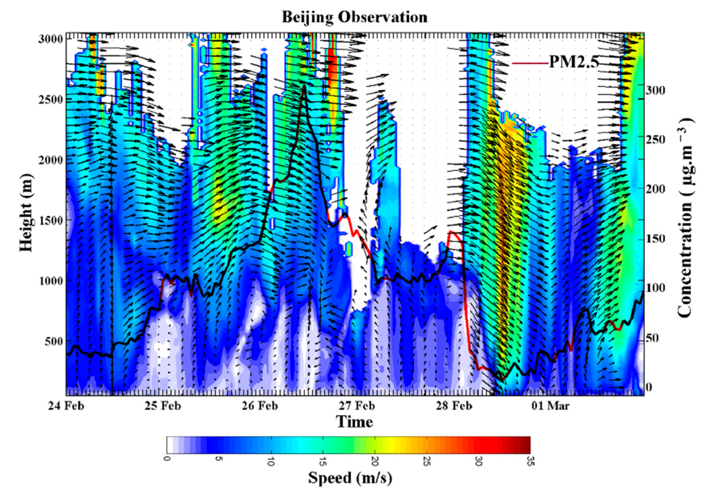
2.1. The DWL Observation

Atmospheric turbulence leads to the fluctuation of the refractive index, the movement of the scattering layer and the movement of turbulence block. It can give rise to turbulence scattering caused by the inhomogeneous refractive index of the atmosphere, resulting in the Doppler frequency shift of the returned electromagnetic wave signal. The radial velocity relative to radar can be obtained using Doppler technology. Under certain assumptions, the wind direction, wind speed and vertical motion at the height of echo signal can be estimated by Doppler multi-direction velocity measurement.
The DWL in this study is the Windcube 100 s DWL, manufactured by Leosphere (France) company. It was deployed in the research area of Institute of Atmospheric Physics, Chinese Academy of Sciences (IAP), located at the urbanization area between the north 3rd and 4th ring roads in Beijing. There are buildings around the observation site, such as the single-storey buildings 15 m away, the 2–3 floor office building about 30 m away, gas stations, residential areas and other buildings 80–100 m away from the observation site, and there are also roads, a river, and large green belts, as shown in Figure 1. The red dots in the picture indicates the location of the experiment.
The DBS scanning mode of vertical observation was adopted. The LiDAR lens transmits four rays at 0°, 90°, 180° and 270° respectively, with a zenith angle of 15° (the angle with vertical direction), and one ray with a vertical direction; thus, the distributions of 3D wind speed and direction at different heights were obtained. The wavelength of the transmitter was 1.5 μm. Its minimum physical resolution was 25 m. According to the principle of DWL, the blind detection area of the instrument was twice the minimum resolution, so it could only monitor the wind field data above 50 m. DWL has good field observation performance, and it can provide 24 h uninterrupted measurements of meteorological elements such as wind velocity, wind direction, temperature and atmospheric refractive index from 50 m to 3000 m above the surface, with a sampling resolution per 20 s. Following the detection method of Brewster K A [16], the accuracy of the DWL data was verified using the special meteorological observation tower, belonging to the IAP, and the missing DWL data caused by strong noise in the near ground signal were eliminated. The tower is 325 m high, divided into 15 layers, and can provide high-quality observation data for Atmospheric Research and measure wind direction and speed.

2.2. Experimental Design

WRF3.9 was used in this study. We conducted a set of model experiments, corresponding to the 11 PBL schemes discussed in the context. Their abbreviations are YSU, MYJ, GFS, QNSE, MYNN2.5, MYNN3, ACM2, BouLac, UW, Shin-Hong, and GBM (Table 1). These schemes correspond to either local or nonlocal closure.
Local closure estimates the unknown PBL quantities by the physical quantities or gradients, through predicting the turbulence perturbation kinetic energy (TKE) at the same place, while nonlocal closure estimates quantities with many known physical quantities or gradients besides the unknown grid. The K-profile method of first-order closure is employed to address the turbulence closure schemes. YSU and ACM2 are nonlocal schemes, while the others are local schemes.
We set up three nested domains centered at 116.68° E, 39.87° N (Figure 1). The horizontal resolutions were 27, 9 and 3 km, with the domain sizes of 100 × 94, 70 × 67 and 64 × 55, respectively. The outermost domain, d01, covered most of China. The second domain, d02, covered the North China Plain and the northwestern mountainous area, including Beijing city. The third domain is the main research area, and is near the IAP. The atmosphere is divided vertically into 43 layers, including 29 layers below 2 km, and the top layer is at 50 hPa. The physical parameterizations include the Dudhia shortwave radiation scheme, the Rapid Radiative Transfer Model longwave radiation scheme, the Kessler scheme for microphysical processes, and the Grell cumulus convection parameterization scheme. As it is not suitable for this fine resolution, the cumulus convection scheme was only applied in d01 and d02 regions, and was turned off in d03. The model was driven by the NCEP/NCAR reanalysis data and integrated from February 24 to March 2, 2018, with an additional 6 h for spin-up [17]. The model results were output every half an hour.
Table 1. Comparison of 11 planetary boundary layer schemes.
OptionsSchemesClosure MethodsMixing Processes for Unstable Boundary LayersMain Features
1Yonsei University (YSU)NonlocalK-Profile Method, First Order Closed ModelConsiders the influence of the entrainment process at the top of the mixed layer on turbulent transport; the height of PBL depends only on the buoyancy profile [18]
2Mellor-Yamada-Janjic Scheme (MYJ)LocalTurbulent kinetic energy (TKE) closure scheme, 1.5-order closure modelIt was suitable for studying fine PBL structure. The height of PBL was determined by the turbulent energy profile [19]
3NCEP Global Forecast System (GFS)NonlocalFirst-order vertical mixing schemeThe height of the PBL was determined by the iterative bulk Rechardson method from the surface up integration. The diffusion coefficient above the surface was a cubic function of the height of the PBL, and its coefficient value was obtained by the coupled surface flux [20]
4Quasi-normal Scale Elimination (QNSE)LocalTKE Closing Scheme, 1.5 Order Closing ModelThe physical process was complex and suitable for the prediction and simulation of the PBL in the stable layer region [21]
5Mellor-Yamada Nakanishi Niino (MYNN) Level 2.5LocalTKE Closing Scheme, 1.5 Order Closing ModelImprovement of MYNN3 limits the ratio between the main length scale and TKE [22]
6Mellor-Yamada Nakanishi Niino (MYNN) Level 3LocalTKE Closing Scheme, 2 Order Closing ModelConsidered the physical process of condensation, the prediction of mixed layer thickness was improved, the TKE magnitude decreased, and the time bias of fog formation and dissipation prediction was reduced [23]
7Asymmetric Convection Model 2 Scheme (ACM2)Nonlocal +LocalThe upward and downward mixing process were local. First-order Closed ModelThe thermal penetration and wind shear of the entrainment layer were considered in the PBL height under unstable conditions. The height of the PBL was determined by the Richardson number [24]
8Bougeault-Lacarrere Scheme (BouLac)LocalTKE Closing Scheme, 1.5 Order Closing ModelIt could predict the intensity and location of clear-sky turbulence over steep terrain and provide a continuous prediction of turbulent energy intensity [25]
9University of Washington (TKE) Boundary LayerLocalTKE Closing Scheme, 1.5 Order Closing ModelThe introduction of a water vapor conservation variable and explicit entrainment closure was suitable for the case of the dry convective PBL [26]
10Shin-Hong Scale-awareLocalTKE Closing Scheme, 1.5 Order Closing ModelVertical mixing in a stable PBL and free atmosphere was similar to the YSU scheme, and it could also diagnose TKE and mixed length output [27]
11Grenier-Bretherton-McCaaLocalTKE Closing Scheme, 1.5 Order Closing ModelConsidered the entrainment process at the top of the PBL, the cloud cover could be well simulated, and the height of the PBL could be calculated according to the grid point heat [28]
Figure 2 illustrates the observed DWL wind data in our case. The PBL wind was weak below a height of 800 m on February 24–25, indicating a stable boundary air. The PBL wind speed increased in the daytime on February 26, and the wind direction above 1000 m height changed from southwest to northwest. The wind slowed again on February 27 and became strong on February 28. At the middle troposphere, according to the MICAPS 4.0 analysis, a cold high pressure was maintained at 500 hPa over northern China, and the low atmosphere was stable. On February 26, a shallow trough passed through Beijing, resulting in haze weather. From 14:00–17:00 UTC (Coordinated Universal Time) on February 28, a cold front induced an upper gale over Beijing and a gale at the ground at 17:00–20:00 UTC. After a short break with gentle winds, the southwest wind was enhanced at 02:00 UTC on 1 March.
Apparently, the PBL wind structures changed substantially under different weather conditions. To clarify the performances of PBL schemes, we evaluated the model results in three weather types, sunny days (24–25 February), hazy days (26–27 February) and windy days (28 February-1 March). The model results at the same height as the DWL vertical observation were compared. Then the model and observation data were grouped depending on the observed wind speeds (i.e., <5, 5–10, 10–15 and >15 m s–1) and six layer heights (30–100, 100–320, 320–1000, 1000–1500, 1500–2000 and >2000 m) to attain a reliable statistical result. Table 2 lists the paired sample sizes in each group. The statistical quantities for evaluation include the model mean bias, correlation coefficient and standard deviation for the wind speeds and directions between the model results (x) and the observations (y) across N layer heights:
Mean Bias
M B = y ¯ x ¯
x ¯ = 1 N i = 1 N x i                           y ¯ = 1 N i = 1 N y i
Correlation Coefficient
C C = I = 1 N ( y i y ¯ ) ( x i x ¯ ) i = 1 N ( y i y ¯ ) 2 i N ( x i x ¯ ) 2
Standard Deviation
S D = 1 N 1 i = 1 N ( x i x ¯ ) 2

3. Results

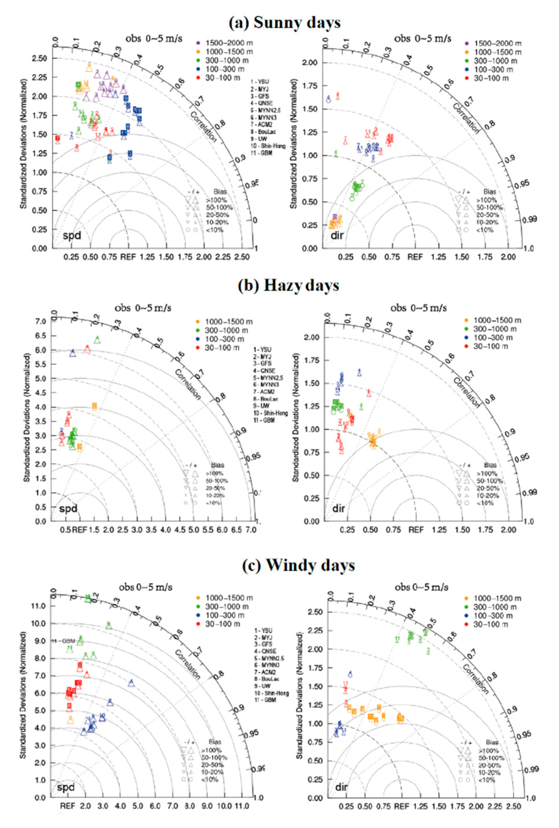
3.1. PBL Wind Speed Profile

Figure 3 shows the PBL wind speed profiles and the model biases with different PBL schemes. The simulated and observed wind speeds varies greatly with altitude. Compared with Figure 2, most of the PBL schemes captured the evolution of wind speed over the days. Figure 4 shows the variation of simulated and observed wind speed with time at an altitude of about 1010 m. During the whole model period, the mean model biases in wind speeds were positive in the layer at 0–1000 m. All PBL schemes had model biases no greater than 10 m·s−1. The model layers near the surface were greatly affected by the roughness length of urban boundary layers which are parameterized in the model with uncertainty. The model biases changed with weather conditions. On hazy days (February 26–27), the observed wind speeds were lower than on the clear days, because the stagnant weather conditions and the aerosol radiative feedback both enhanced the PBL stability and also lowered the surface wind speeds [29]. For example, when the wind speed was 5–10 m·s−1, the simulated wind speed on the hazy days was 1–2 m·s−1 (18–38%) lower than the observed wind speed on each level. On windy days (28 February 28–1 March), the model bias in wind direction decreased along the height. In the layer of 1000–1500 m, the wind direction bias of PBL schemes were 1.1°–9.1° (0.4–3.4%) (except bias of QNSE was 88°, 33.4%).

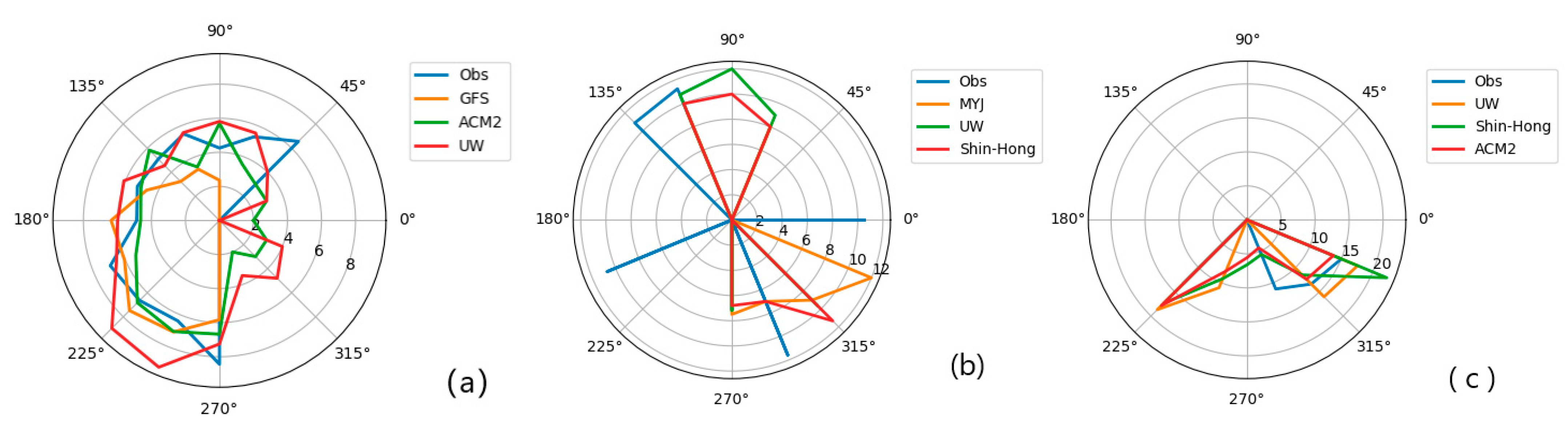
3.2. Horizontal Wind Component in PBL

Figure 5 presents the model biases in the horizontal wind components at each layer for different horizontal speed levels. Generally, all the PBL schemes had model biases in horizontal wind speed smaller than 2 m·s−1, and the biases in wind direction were less than 20°. On gentle windy days with observed wind speed less than 5 m·s−1, the YSU bias reached up to 10 m·s−1. On sunny days and hazy days, the model biases of YSU were large at 1000–1500 m and 1500–2000 m, where the wind speeds exceeded 15 m·s−1. QNSE showed the maximum model bias in wind speeds, particularly on haze and windy days. On windy days, the biases in wind direction were about 80° or even more than 100° at heights of 300–1000 m, 1000–1500 m, and 1500–2000 m. Meanwhile, the biases of other PBL schemes were within 20°. The MYJ scheme performed well in the wind speed simulation, but overestimated the wind direction by about 280% below 300 m. At wind speed level of 5–10 m·s−1, the biases in wind direction were over 100° for the YSU, GFS, MYNN2.5, MYNN3 and BouLac schemes. The model bias also increased with height, particularly when the observed wind speeds were less than 5 m·s−1. On hazy days, when the wind speed was less than 5 m·s−1, the wind direction biases for these PBL schemes were more than 180° at 1500–2000 m. Table 3 shows the biases of the PBL scheme for a specific height and wind speed interval. At 1000–1500 m and 1500–2000 m altitude, the simulated standard deviation was large when the observed wind speeds exceeded 15 m·s−1 or were less than 5 m·s−1. The QNSE schemes gave a reasonable wind speed and direction value on sunny days, but the model results became worse on hazy and windy days. On windy days, the QNSE scheme led to standard deviations of wind directions at 300–2000 m of up to 80°, or even more than 100°, while the other schemes had biases within 20°. The MYJ scheme well simulated the wind speed, but the variation of wind direction below 300 m reached up to about 280%. The variations of wind directions when using the YSU, GFS, MYNN2.5, MYNN3 and BouLac schemes were over 100° in the wind speed level of 5–10 m·s−1. On hazy days, for wind speeds less than 5 m·s−1, the simulated standard deviations of wind direction were more than 180° at a height of 1500–2000 m. In Table 3, ①②③④⑤⑥⑦⑧⑨⑩⑪ represent 11 different boundary layer schemes; these are YSU, MYJ, GFS, QNSE, MYNN2.5, MYNN3, ACM2, BouLac, UW, SH, GBM. The figure shows the simulation effect of wind speed and direction in different wind speed segments (0–5, 5–10, 10–15, greater than 15) under three weather conditions (sunny day, fog, strong wind) at different heights (below 100, 100–300, 300–1000, 1000–1500, 1500–2000, and over 2000 m). For the convenience of comparison, the simulated height is consistent with the horizontal height of the observation point. Therefore, the altitude here represents both the observed altitude and the simulated altitude. Additionally, only schemes with wind speed or direction biases lower than 20% can be shown in the table. According to Table 3, for example, on sunny days, when the height was less than 100 m, and the observed wind speed was less than 5, the wind speed biases of scheme ③ were less than 20%, and when the wind speed was between 5 and 10, the wind speed bias of schemes ③ and ⑨ were less than 20%, which indicates that the simulation effects of the PBL schemes were better.
In Figure 6, a comparison is made between the wind field observed near the ground and the simulated wind field with two PBL schemes under the same conditions, with a wind speed of 5–10 m·s−1 on sunny days. Figure 7 shows a comparison between different wind speeds and height schemes under three weather conditions. Better results for the scheme simulations are presented. We can see from the chart that the wind direction and wind speed simulations cover the observation results, but there were still biases, sometimes up to 45°–60°.
Obs stands for observation wind field, the GFS scheme simulates the wind field, with wind speed and wind direction bias of 0.68 m·s−1 and 9.8°, respectively, the BouLac scheme simulates wind field, with wind speed and wind direction biases of −1.1 m·s−1, 0.8°.
Figure 8 exhibits the Taylor chart for the model results at different heights and wind speeds when the observed wind speed is at 0–5 m·s−1. The Taylor charts show similar characteristics to the other observed wind speeds (i.e., 5–10, 10–15 and >15 m·s−1). The correlation coefficients that failed to pass the significance test with the significance level of 0.05 are not shown in the figure. The horizontal and vertical coordinates represent the ratio of the standard deviation of the simulated value to the standard deviation of the observed value. A ratio of 1 indicates that the standard deviation was perfect. The gray arc represents the isoline with equal distance between each point and the point with a standard deviation of 1. In the left and right columns of the figure, ‘spd’ in the lower left corner stands for the comparison of wind speed between the simulated value and the observed value, and ‘dir’ represents the comparison of wind direction. Obs represents the actual wind speed range of the analysis data in the graph. The cases with coefficients that failed to pass the significance test on the three different kinds of days do not appear in the figures.
As can be seen from Figure 8, each wind speed segment could have suitable simulation schemes for each height. Biases and standard deviation should also be considered comprehensively. For example, when the Obs was 5–10 m·s−1, the standard deviation at 100–300 m was approximately 20 times higher than the observation standard deviation. The correlation at 300–1000 m was approximately as weak as 0.1–0.2, while at 1000–1500 m, there was the non-pass hypothesis test. On windy days, when Obs was 0–5 m·s−1, the simulated value of wind speed was several times the standard deviation of the observed value, and the bias value was greater than 100%.

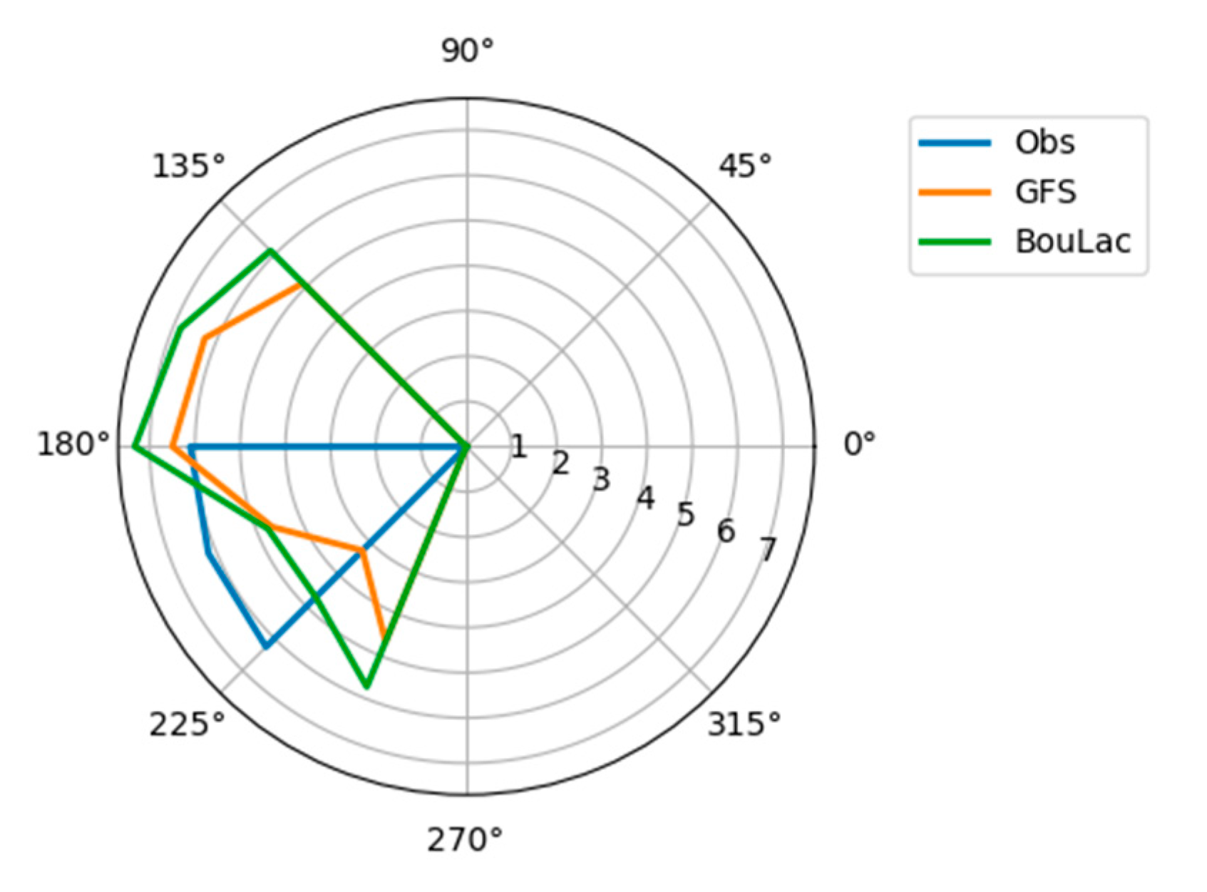
3.3. Classical PBL Schemes

As is shown in Section 1, many previous studies have indicated that YSU, MYJ, ACM2 showed good simulation results. In this study, the PBL conditions changed with the weather evolution, and they were not always stable or unstable. On windy days, with an observed wind speed of 5–10 m·s−1 and at a height greater than 300 m, the YSU bias of wind speed was 50–70%. On sunny days, when the observed wind speed was less than 5 m·s−1, the MYJ mean bias of wind speed was within the range of 60–290%. A few studies have claimed that the QNSE scheme is suitable in stable conditions, which was also proved in our results. We found that the QNSE scheme performed poorly on windy days, but showed better results on sunny days and hazy days, especially for the observed wind speed exceeding 5 m·s−1 at layers above 2000 m. The above performances further prove that a scheme cannot be fully suitable for certain weather conditions.
The YSU and MYJ schemes, widely applied in previous studies, also presented good performances in our studies. The YSU scheme may be a good choice under the following conditions: to simulate the surface wind direction for observed wind speeds stronger than 5 m·s−1, or to simulate the wind direction above 300 m on sunny and hazy days, and perhaps to simulate wind speed below 300 m on windy days. It can also be used to simulate the wind direction above 300 m, the wind speed simulation above 1000 m, the wind speed simulation of over 15 m·s−1, and the simulation of wind direction at 5–15 m·s−1.
The MYJ scheme was considered suitable for the following conditions. For example, to simulate wind speed below 300 m when the wind speed is more than 5 m·s−1 on sunny days, or to simulate the winds at 300–1000 m, and perhaps to simulate the wind direction when the height is greater than 1000 m, maybe also on windy days when the wind speed is within the range 10–15 m·s−1 and the altitude is greater than 2000 m. Additionally, the MYJ scheme is able to well capture both wind speed and direction on hazy days when the wind speed is 10–15 m·s−1 at 300–1000 m.
In other words, suitable PBL schemes should be chosen for different conditions. In this case, on sunny days, when Obs was 0–5 m·s−1, we found that the wind speed was simulated well at the height 100–300 m, and the wind direction simulation performed well at 300–1000 m. When the Obs was 5–10 m·s−1, the wind speed at 100–300 m was better than at 300–1000 m. When the Obs was 10–15 m·s−1, the wind speed data were mainly distributed in the upper 1000 m; while little data at 1000–2000 m satisfied the hypothesis test, many data satisfied hypothesis test at heights above 2000 m. At this altitude, schemes 7 and 12 can be used. Wind speeds greater than 15 m·s−1 were mainly distributed at heights above 1500 m, and schemes 2, 4, 7 and 11 could be selected. On hazy days, when the height was above 1000 m, the simulation results of several schemes were better. When the Obs was less than 5 m·s−1 and the height was 1000–1500 m, the wind direction could be simulated with PBL schemes 2 and 3, and the wind speed simulation at 300–1000 m was relatively good. Above 2000 m, the simulation results could not be verified completely due to limited observation data. It turns out that no PBL scheme always shows good performances.

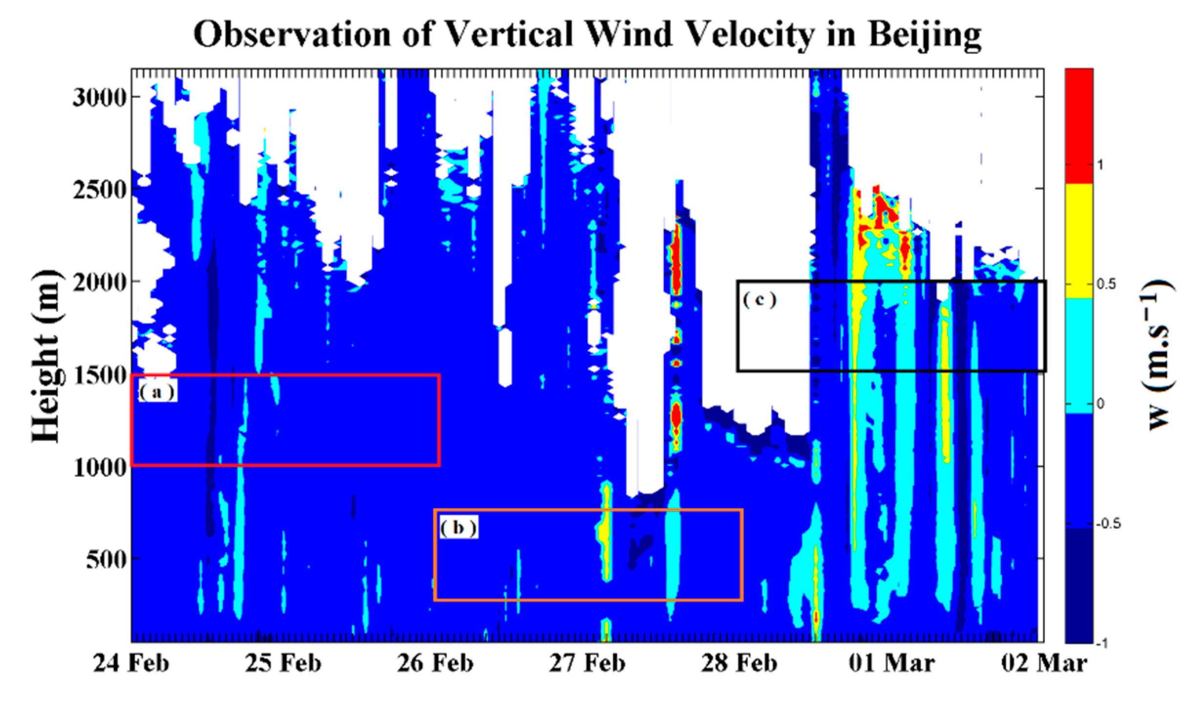
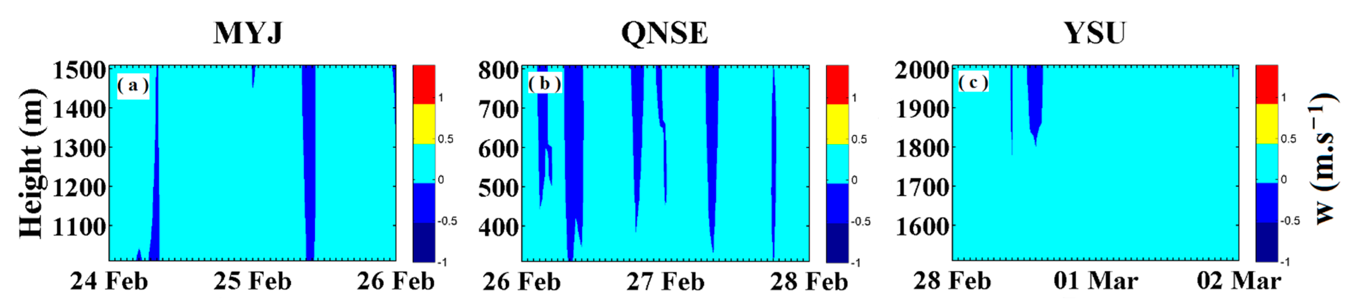
3.4. Vertical Wind Component in PBL

Figure 9 shows the observation and the simulated vertical wind speeds with three PBL schemes according to the observed vertical wind field. On sunny days and hazy days, the simulated wind speed values were 10% of the observation value, and the wind speed was mostly distributed between 0 and 0.5 under the boundary layer, and the wind direction was vertical downward. However, the simulation results show that the wind direction was mainly vertical upward. On the windy days from 28 February to 1 March, there was strong upward turbulence from the surface to the upper air in the vertical direction, and the maximum wind speed was more than 0.5 m·s−1.
The model failed to capture the change in vertical wind speeds (Figure 10), not only as a consequence of the model’s uncertainty, but also potentially due to the biases in the DWL data. It is known that, under a clear sky, the updraft and downdraft of airflow are small. The turbulence echo approached the detection limit of the Doppler LiDAR, which makes an accurate extraction of vertical wind speed difficult.

4. Conclusions

In this study, the accuracy of the vertical wind field simulation for different boundary layer schemes was systematically evaluated using high-resolution wind Doppler LiDAR for the first time, with a typical process simulated by a WRF model in Beijing. The results showed that the wind field was simulated well at a height of 1000–2000 m, as most of the relative mean biases of wind speed and wind direction were less than 20% and 6%, respectively. Below 1000 m, the wind speed and direction biases ranged from about 30% to more than 150% m·s−1 and 6–30%, respectively. The relative mean bias of the simulated wind profile was up to 50–300% when the wind speed was lower than 5 m·s−1 in the boundary layer. As the wind speed range was 10–15 m·s−1, the model results were better than for other speeds, and were better when the height was above 1000 m. The PBL schemes have different capabilities to reproduce the changes of wind speed profiles under different weather conditions. An appropriate PBL scheme is dependent on the weather conditions, and the model biases showed substantial changes at different heights and in different wind speed ranges, and some PBL schemes were not always likely to be suitable for a certain weather condition. The influence of observation height on the assessment was larger than that due to employing the different PBL schemes. This study provides a reference for further improving the development and use of wind energy and the accuracy of complex wind field predictions.

Author Contributions

J.X. and Y.Y. designed the experiments and the research. W.C., M.X., D.J., Y.M. provided experimental assistance and the analytical method. L.Z. and J.X. analyzed the data and performed research. All authors commented on the manuscript. All authors have read and agreed to the published version of the manuscript.

Funding

This study was partially supported by the CAS Strategic Priority Research Program (XDA23020301), the National Key Research and Development Program of China (2016YFC0202001) and the National Natural Science Foundation of China (42061130215).

Informed Consent Statement

Informed consent was obtained from all subjects involved in the study.

Conflicts of Interest

The authors declare no conflict of interest.

References

  1. Coantic, M.; Seguin, B. On the interaction of turbulent and radiative transfers in the surface layer. Bound. Layer Meteorol. 1971, 1, 245–263. [Google Scholar] [CrossRef]
  2. Cheng, F.Y.; Chin, S.C.; Liu, T.H. The role of boundary layer schemes in meteorological and air quality simulations of the Taiwan area. Atmos. Environ. 2012, 54, 714–727. [Google Scholar] [CrossRef]
  3. Han, Z.; Zhang, M.; An, J. Sensitivity of air quality model prediction to parameterization of vertical eddy diffusivity. Environ. Fluid Mech. 2008, 9, 73–89. [Google Scholar] [CrossRef]
  4. Wei, J.; Tang, G.; Zhu, X.; Wang, L.; Liu, Z.; Cheng, M.; Münkel, C.; Li, X.; Wang, Y. Thermal internal boundary layer and its effects on air pollutants during summer in a coastal city in North China. J. Environ. Sci. 2017, 70, 37–44. [Google Scholar] [CrossRef] [PubMed]
  5. Wang, Z.; Cao, X.; Zhang, L.; Notholt, J.; Zhou, B.; Liu, R.; Zhang, B. Lidar measurement of planetary boundary layer height and comparison with microwave profiling radiometer observation. Atmos. Meas. Tech. 2012, 5, 1965–1972. [Google Scholar] [CrossRef] [Green Version]
  6. Zhang, C.; Wang, D.; Gong, Y. Dynamic Modeling Study of Highly Resolved Near-Surface Wind Based on WRF/CALMET. Meteorol. Mon. 2015, 1, 34–44. [Google Scholar]
  7. Zhan, L.; Shu, J.; Chen, L. Distribution characteristics of wind and pollutant concentration fields in a parallel urban block. J. Meteorol. Environ. 2017, 33, 61–67. [Google Scholar]
  8. Hahmann, A.N.; Draxl, C.; Peña, A.; Nielsen, J.R. Simulating the Vertical Structure of the Wind with the Weather Research and Forecasting (WRF) Model; European Wind Energy Conference and Exhibition: EWEA 2011; Europe’s Premier Wind Energy Event: Brussels, Belgium, 2011; p. 153. [Google Scholar]
  9. Gholami, S.; Ghader, S.; Khaleghi-Zavareh, H.; Ghafarian, P. Sensitivity of WRF-simulated 10 m wind over the Persian Gulf to different boundary conditions and PBL parameterization schemes. Atmos. Res. 2020, 247, 105147. [Google Scholar] [CrossRef]
  10. Fekih, A.; Mohamed, A. Evaluation of the WRF model on simulating the vertical structure and diurnal cycle of the atmospheric boundary layer over Bordj Badji Mokhtar (southwestern Algeria). J. King Saud Univ. Sci. 2019, 31, 602–611. [Google Scholar] [CrossRef]
  11. Miglietta, M.M.; Zecchetto, S.; De Biasio, F. WRF model and ASAR-retrieved 10 m wind field comparison in a case study over Eastern Mediterranean Sea. Adv. Sci. Res. 2010, 4, 83–88. [Google Scholar] [CrossRef]
  12. Shimada, S.; Ohsawa, T.; Chikaoka, S.; Kozai, K. Accuracy of the wind speed profile in the lower PBL as simulated by the WRF model. Sola 2011, 7, 109–112. [Google Scholar] [CrossRef] [Green Version]
  13. Banks, R.F.; Tiana-Alsina, J.; Rocadenbosch, F.; Baldasano, J.M. Performance Evaluation of the Boundary-Layer Height from Lidar and the Weather Research and Forecasting Model at an Urban Coastal Site in the North-East Iberian Peninsula. Bound. Layer Meteorol. 2015, 157, 265–292. [Google Scholar] [CrossRef] [Green Version]
  14. Banks, R.; Baldasano, J. Impact of WRF model PBL schemes on air quality simulations over Catalonia, Spain. Sci. Total Environ. 2016, 572, 98–113. [Google Scholar] [CrossRef] [PubMed] [Green Version]
  15. Muñoz-Esparza, D.; Cañadillas, B.; Neumann, T.; Beeck, J.V. Turbulent fluxes, stability and shear in the offshore environment: Mesoscale modelling and field observations at FINO1. J. Renew. Sustain. Energy 2012, 4, 063136. [Google Scholar] [CrossRef]
  16. Brewster, K.A. Profiler Training Manual #2: Quality Control of Wind Profiler Data; NOAA/ERL/FSL: Boulder, CO, USA; NOAA/NWS/OM: Silver Spring, MD, USA, 1989; p. 109. [Google Scholar]
  17. Clark, A.J.; Gallus, W.A.; Chen, T.C. Comparison of the Diurnal Precipitation Cycle in Convection-Resolving and Non-Convection-Resolving Mesoscale Models. Mon. Weather Rev. 2007, 135, 3456–3473. [Google Scholar] [CrossRef] [Green Version]
  18. Hong, S.Y.; Noh, Y.; Dudhia, J. A New Vertical Diffusion Package with an Explicit Treatment of Entrainment Processes. Mon. Weather. Rev. 2005, 134, 2318–2341. [Google Scholar] [CrossRef] [Green Version]
  19. Janjic, Z.I. The Step-Mountain Eta Coordinate Model: Further Developments of the Convection, Viscous Sublayer, and Turbulence Closure Schemes. Mon. Weather Rev. 1994, 122, 927. [Google Scholar] [CrossRef] [Green Version]
  20. Hong, S.Y.; Pan, H.L. Nonlocal Boundary Layer Vertical Diffusion in a Medium-Range Forecast Model. Mon. Weather Rev. 1996, 124, 2322–2339. [Google Scholar] [CrossRef] [Green Version]
  21. Sukoriansky, S.; Galperin, B.; Perov, V. Application of a New Spectral Theory of Stably Stratified Turbulence to the Atmospheric Boundary Layer over Sea Ice. Bound. Layer Meteorol. 2005, 117, 231–257. [Google Scholar] [CrossRef]
  22. Nakanishi, M.; Niino, H. An Improved Mellor–Yamada Level-3 Model: Its Numerical Stability and Application to a Regional Prediction of Advection Fog. Bound. Layer Meteorol. 2006, 119, 397–407. [Google Scholar] [CrossRef]
  23. Mikio, N.; Hiroshi, N. Development of an Improved Turbulence Closure Model for the Atmospheric Boundary Layer. J. Meteorol. Soc. Jpn. 2009, 87, 895–912. [Google Scholar] [CrossRef] [Green Version]
  24. Pleim, J.E. A Combined Local and Nonlocal Closure Model for the Atmospheric Boundary Layer. Part I: Model Description and Testing. J. Appl. Meteorol. Clim. 2007, 46, 1383–1395. [Google Scholar] [CrossRef]
  25. Bougeault, P.; Lacarrere, P. Parameterization of Orography-Induced Turbulence in a Mesobeta-Scale Model. Mon. Weather Rev. 1989, 117, 1872–1890. [Google Scholar] [CrossRef]
  26. Bretherton, C.S.; Park, S. A New Moist Turbulence Parameterization in the Community Atmosphere Model. J. Clim. 2009, 22, 3422–3448. [Google Scholar] [CrossRef]
  27. Shin, H.H.; Hong, S. Representation of the Subgrid-Scale Turbulent Transport in Convective Boundary Layers at Gray-Zone Resolutions. Mon. Weather Rev. 2015, 143, 250–271. [Google Scholar] [CrossRef]
  28. Grenier, H.; Bretherton, C.S. A Moist PBL Parameterization for Large-Scale Models and Its Application to Subtropical Cloud-Topped Marine Boundary Layers. Mon. Weather Rev. 2001, 129, 357. [Google Scholar] [CrossRef] [Green Version]
  29. Sun, K.; Liu, H.; Wang, X.; Peng, Z.; Xiong, Z. The Aerosol Radiative Effect on a Severe Haze Episode in the Yangtze River Delta. J. Meteorol. Res. 2017, 31, 59–67. [Google Scholar] [CrossRef] [Green Version]
Figure 1. Location of the experimental site in this study.
Atmosphere 12 00777 g001
Figure 2. The model topography (left, middle) and the schematic diagram of the DWL (right) deployed in the center of model domain (red point in the left).
Atmosphere 12 00777 g002
Figure 3. The simulated PM2.5 concentrations (red line) and the PBL wind structures in Beijing, February 2018.
Atmosphere 12 00777 g003
Figure 4. The wind field simulations (af) with the PBL schemes of YSU, MYJ, QNSE, BouLac, UW and Shin-Hong Schemes and their biases (gn) against the observations. The sunny, haze and windy days were on 24–25 February, 26–27 February and 28 February to 1 March, respectively.
Atmosphere 12 00777 g004
Figure 5. The observed and simulated wind speeds at a height of 1010 m with the PBL schemes of YSU, MYJ, QNSE, BouLac, UW and SH.
Atmosphere 12 00777 g005
Figure 6. The model biases in wind speed (left, bias less than 2 m·s−1) and wind direction (right, bias less than 20°) depending on the PBL schemes, the layer heights and the wind speeds on sunny, haze and windy days.
Atmosphere 12 00777 g006
Figure 7. Wind field comparison chart. The observed wind speed is 5–10 m·s−1, and the height is 100–300 m on the 24th–25th (sunny days).
Atmosphere 12 00777 g007
Figure 8. Wind field comparison chart, the observed wind field and simulated wind field with several PBL schemes under different conditions. (a) On sunny days, at a height of 300–1000 m, 5 < Obs <10 m·s−1, (b) On hazy days, at a height of 300–1000 m, 10 < Obs < 15 m·s−1, (c) On windy days, at a height of 1000–1500 m, 10 < Obs < 15 m·s−1.
Atmosphere 12 00777 g008
Figure 9. Taylor charts of mean bias, correlation coefficients and standard deviations for the model results with 11 PBL schemes. On (a) sunny days, (b) hazy days, and (c) windy days, with the observed wind speed at 0–5 m·s−1.
Atmosphere 12 00777 g009
Figure 10. Comparison of vertical wind speeds between the observations and the simulations using (a) the GFS scheme at 1000–1500 m height on sunny days, (b) the MYNN3 scheme at 300–800 m height on hazy days, and (c) the UW scheme at 1500–2000 m height on windy days.
Atmosphere 12 00777 g010aAtmosphere 12 00777 g010b
Table 2. The DWL sample size in data groups.
Weather ConditionsObs (m s−1)30–100 m100–300 m300–1000 m1000–1500 m1500–2000 m2000–3000 m
Sunny days0–5239342653249870
5–1019092371940372
10–150056175479748
>1500034131261
Hazy days0–524042010564430
5–1000480139628
10–150034270553463
>1500027142424
Windy days0–5205257607135860
5–10341104933141468
10–15129224221300210
>1502308357324271
Table 3. Under different conditions, the PBL schemes with low biases of wind speed and direction, large correlation coefficients, and close standard deviation on sunny days, hazy days and windy days, and at four wind speeds ranges (0–5, 5–10, 10–15, over 15). The bias of suitable scheme in the table is below 20%. “—” Indicates poor simulation or no data. “All” means all the PBL schemes.
Wind Speed Simulation
Height (m)Obs (m·s−1)
0–55–1010–15>15
Sunny days<100③⑨
100–300①③⑤⑥⑧⑩⑪①②③④⑤⑥⑧⑨⑩⑪
300–1000②③④⑨
1000–1500③④①⑤⑥⑧⑨⑩⑪
1500–2000⑦⑧⑪
>2000All
Hazy days<100②⑧⑪
100–300All
300–1000③⑧⑪①②④⑨⑩
1000–1500②③①⑤⑥⑦⑧⑨⑩⑪
1500–2000②③④⑤⑥⑧⑨⑪①⑥⑦⑩⑪①④⑤⑥⑦⑧⑨⑩⑪
>2000①②③⑤⑦⑧⑨⑩⑪①②③⑤⑥⑦⑧⑨⑩⑪
Windy days<100①⑩①⑤⑥⑩
100–300All①⑤⑥⑦⑩①⑨⑩⑪
300–1000④⑧②③⑤⑥⑦⑨⑩
1000–1500④⑤⑥⑤⑥③⑤⑥⑦⑧⑨⑪①③⑨⑩
1500–2000③⑦⑧⑨⑪①③⑨⑩
>2000②⑦⑪
Wind Direction Simulation
Height (m)Obs (m·s−1)
0–55–1010–15>15
Sunny days<100①②④
100–300①②③⑤⑥⑧⑨⑩⑪
300–1000①②③⑤⑥⑨⑩⑪All
1000–1500④⑤⑧⑨⑪①②③⑤⑥⑦⑧⑨⑩⑪①⑤⑥⑧⑨⑩⑪
1500–2000①③⑧⑩⑪⑦⑧⑪①③⑤⑥⑦⑧⑨⑩⑪
>2000①③⑦⑧⑨⑩⑪①③⑤⑥⑦⑧⑨⑩⑪①②③⑤⑥⑧⑨⑩
Hazy days<100⑤⑥
100 - 300⑤⑥⑨①②④⑤⑥⑧
300 -1000③⑧⑨①③④⑤⑥⑦⑧⑨⑩⑪‘①②③⑤⑥⑦⑧⑨⑩⑪
1000–1500
1500–2000①④⑤⑥⑦⑧⑨⑩⑪
>2000①②③⑤⑥⑦⑧⑨⑩⑪All
Windy days<100①④⑨⑩
100–300
300–1000①②③⑤⑥⑦⑧⑨⑩⑪①⑦⑩
1000–1500①②③⑤⑥⑦⑧⑨⑩⑪①②③⑤⑥⑦⑧⑨⑩⑪②⑤⑥⑦⑧
1500–2000①②③⑦⑩⑪①⑧⑩③⑧⑩⑪②③⑤⑥⑦⑧⑨⑪
>2000①③⑥⑦⑧⑩⑪②⑨⑪
Publisher’s Note: MDPI stays neutral with regard to jurisdictional claims in published maps and institutional affiliations.

